Conformal Random Geometry
1 Preamble
In these Lecture Notes11 1 These Notes are based on my previous research survey article published in Ref. [1], augmented by introductory sections, explanatory figures and some new material. Supplementary technical Appendices can be found in Ref. [1], or in the forecoming extended version of the present Lectures on the Cornell University Library web site, arXiv.org., a comprehensive description of the universal fractal geometry of conformally-invariant (CI) scaling curves or interfaces, in the plane or half-plane, is given. They can be considered as complementary to those by Wendelin Werner.22 2 W. Werner, Some Recent Aspects of Random Conformally Invariant Systems [2]; see also [3].
The present approach focuses on deriving critical exponents associated with interacting random paths, by exploiting an underlying quantum gravity (QG) structure. The latter relates exponents in the plane to those on a random lattice, i.e., in a fluctuating metric, using the so-called Knizhnik, Polyakov and Zamolodchikov (KPZ) map. This is accomplished within the framework of random matrix theory and conformal field theory (CFT), with applications to well-recognized geometrical critical models, like Brownian paths, self-avoiding walks, percolation, and more generally, the or -state Potts models, and Schramm’s Stochastic Löwner Evolution ().33 3 For an introduction, see the recent book by G. F. Lawler [4].
Two fundamental ingredients of the QG construction are: the relation of bulk to Dirichlet boundary exponents, and additivity rules for QG boundary conformal dimensions associated with mutual-avoidance between sets of random paths. These relation and rules are established from the general structure of correlation functions of arbitrary interacting random sets on a random lattice, as derived from random matrix theory.
The additivity of boundary exponents in quantum gravity for mutually-avoiding paths is in contradistinction to the usual additivity of exponents in the standard complex plane or half-plane , where the latter additivity corresponds to the statistical independence of random processes, hence to possibly overlapping random paths. Therefore, with both additivities at hand, either in QG or in (or ), and the possibility of multiple, direct or inverse, KPZ-maps between the random and the complex planes, any entangled structure made of interacting paths can be resolved and its exponents calculated, as explained in these Notes.
From this, non-intersection exponents for random walks or Brownian paths, self-avoiding walks (SAW’s), or arbitrary mixtures thereof are derived in particular.
Next, the multifractal function of the harmonic measure (i.e., electrostatic potential, or diffusion field) near any conformally invariant fractal boundary or interface, is obtained as a function of the central charge of the associated CFT. It gives the Hausdorff dimension of the set of frontier points , where the potential varies with distance to the said point as . From an electrostatic point of view, this is equivalent to saying that the frontier locally looks like a wedge of opening angle , with a potential scaling like , whence . Equivalently, the electrostatic charge contained in a ball of radius centered at , and the harmonic measure, i.e., the probability that an auxiliary Brownian motion started at infinity, first hits the frontier in the same ball, both scale like .
In particular, we shall see that Brownian paths, SAW’s in the scaling limit, and critical percolation clusters all have identical spectra corresponding to the same central charge . This result therefore states that the frontiers of a Brownian path or of the scaling limit of a critical percolation cluster are just identical with the scaling limit of a self-avoiding walk (or loop).
Higher multifractal functions, like the double spectrum of the double-sided harmonic measure on both sides of an SLE, are similarly obtained.
As a corollary, the Hausdorff dimension of a non-simple scaling curve or cluster hull, and the dimension of its simple frontier or external perimeter, are shown to obey the (superuniversal) duality equation , valid for any value of the central charge .
For the process, this predicts the existence of a duality which associates simple ( SLE paths as external frontiers of non-simple paths ( paths. This duality is established via an algebraic symmetry of the KPZ quantum gravity map. An extended dual KPZ relation is thus introduced for the SLE, which commutes with the duality.
Quantum gravity allows one to “transmute” random paths one into another, in particular Brownian paths into equivalent SLE paths. Combined with duality, this allows one to calculate SLE exponents from simple QG fusion rules.
Besides the set of local singularity exponents introduced above, the statistical description of the random geometry of a conformally invariant scaling curve or interface requires the introduction of logarithmic spirals. These provide geometrical configurations of a scaling curve about a generic point that are conformally invariant, and correspond to the asymptotic logarithmic winding of the polar angle at distance , , of the wedge (of opening angle ) seen above.
In complex analysis and probability theory, this is best described by a new multifractal spectrum, the mixed rotation harmonic spectrum , which gives the Hausdorff dimension of the set of points possessing both a local logarithmic winding rate and a local singularity exponent with respect to the harmonic measure.
The spectrum of any conformally invariant scaling curve or interface is thus obtained as a function of the central charge labelling the associated CFT, or, equivalently, of the parameter for the process. Recently, these results have been derived rigorously, including their various probabilistic senses, from first principle calculations within the SLE framework, thus vindicating the QG approach.
The Lecture Notes by Wendelin Werner in this volume [2] are based on the rigorous construction of conformal ensembles of random curves using the SLE. Bridging the gap between these physics and mathematics based approaches should constitute an interesting project for future studies.
A first step is the reformulation of the probabilistic SLE formalism in terms of standard conformal field theory.44 4 For an introduction, see M. Bauer and D. Bernard [5], and J. Cardy, SLE for Theoretical Physicists, [6]. A second one would be a more direct relation to standard models and methods of statistical mechanics in two dimensions like the Coulomb gas and Bethe Ansatz ones.55 5 See, e.g., W. Kager and B. Nienhuis [7]. The natural emergence of quantum gravity in the SLE framework should be the next issue.
Let us start with a brief history of conformal invariance in statistical physics and probability theory.
2 Introduction
2.1 A Brief Conformal History
Brownian Paths, Critical Phenomena, and Quantum Field Theory
Brownian motion is the archetype of a random process, hence its great importance in physics and probability theory [8]. The Brownian path is also the archetype of a scale invariant set, and in two dimensions is a conformally-invariant one, as shown by P. Lévy [9]. It is therefore perhaps the most natural random fractal [10]. On the other hand, Brownian paths are intimately linked with quantum field theory (QFT). Intersections of Brownian paths indeed provide the random geometrical mechanism underlying QFT [11]. In a Feynman diagram, any propagator line can be represented by a Brownian path, and the vertices are intersection points of the Brownian paths. This equivalence is widely used in polymer theory [12, 13] and in rigorous studies of second-order phase transitions and field theories [14]. Families of universal critical exponents are in particular associated with non-intersection probabilities of collections of random walks or Brownian paths, and these play an important role both in probability theory and quantum field theory [15, 16, 17, 18].
A perhaps less known fact is the existence of highly non-trivial geometrical, actually fractal (or multifractal), properties of Brownian paths or their subsets [10]. These types of geometrical fractal properties generalize to all universality classes of, e.g., random walks (RW’s), loop-erased random walks (LERW’s), self-avoiding walks (SAW’s) or polymers, Ising, percolation and Potts models, models, which are related in an essential way to standard critical phenomena and field theory. The random fractal geometry is particularly rich in two dimensions.
Conformal Invariance and Coulomb Gas
In two dimensions (2D), the notion of conformal invariance [19, 20, 21], and the introduction of the so-called “Coulomb gas techniques” and “Bethe Ansatz” have brought a wealth of exact results in the Statistical Mechanics of critical models (see, e.g., Refs. [22] to [51]). Conformal field theory (CFT) has lent strong support to the conjecture that statistical systems at their critical point, in their scaling (continuum) limit, produce conformally-invariant (CI) fractal structures, examples of which are the continuum scaling limits of RW’s, LERW’s, SAW’s, critical Ising or Potts clusters. A prominent role was played by Cardy’s equation for the crossing probabilities in 2D percolation [43]. To understand conformal invariance in a rigorous way presented a mathematical challenge (see, e.g., Refs. [52, 53, 54]).

In the particular case of planar Brownian paths, Benoît Mandelbrot [10] made the following famous conjecture in 1982: in two dimensions, the external frontier of a planar Brownian path has a Hausdorff dimension
| (2.1) |
identical to that found by B. Nienhuis for a planar self-avoiding walk [24]. This identity has played an important role in probability theory and theoretical physics in recent years, and will be a central theme in these Notes. We shall understand this identity in the light of “quantum gravity”, to which we turn now.

Quantum Gravity and the KPZ Relation
Another breakthrough, not widely noticed at the time, was the introduction of “2D quantum gravity” (QG) in the statistical mechanics of 2D critical systems. V. A. Kazakov gave the solution of the Ising model on a random planar lattice [55]. The astounding discovery by Knizhnik, Polyakov, and Zamolodchikov of the “KPZ” map between critical exponents in the standard plane and in a random 2D metric [56] led to the relation of the exponents found in Ref. [55] to those of Onsager (see also [57]). The first other explicit solutions and checks of KPZ were obtained for SAW’s [58] and for the model [59, 60, 61].
Multifractality
The concepts of generalized dimensions and associated multifractal (MF) measures were developed in parallel two decades ago [62, 63, 64, 65]. It was later realized that multifractals and field theory have deep connections, since the algebras of their respective correlation functions reveal striking similarities [66].
A particular example is given by classical potential theory, i.e., that of the electrostatic or diffusion field near critical fractal boundaries, or near diffusion limited aggregates (DLA). The self-similarity of the fractal boundary is indeed reflected in a multifractal behavior of the moments of the potential. In DLA, the potential, also called harmonic measure, actually determines the growth process [67, 68, 69, 70]. For equilibrium statistical fractals, a first analytical example of multifractality was studied in ref. [71], where the fractal boundary was chosen to be a simple RW, or a SAW, both accessible to renormalization group methods near four dimensions. In two dimensions, the existence of a multifractal spectrum for the Brownian path frontier was established rigorously [72].
In 2D, in analogy to the simplicity of the classical method of conformal transforms to solve electrostatics of Euclidean domains, a universal solution could be expected for the distribution of potential near any CI fractal in the plane. It was clear that these multifractal spectra should be linked with the conformal invariance classification, but outside the realm of the usual rational exponents. That presented a second challenge to the theory.
2.2 Conformal Geometrical Structures
Brownian Intersection Exponents
It was already envisioned in the mid-eighties that the critical properties of planar Brownian paths, whose conformal invariance was well-established [9], could be the opening gate to rigorous studies of two-dimensional critical phenomena.66 6 It is perhaps interesting to note that P.-G. de Gennes originally studied polymer theory with the same hope of understanding from that perspective the broader class of critical phenomena. It turned out to be historically the converse: the Wilson-Fisher renormalization group approach to spin models with symmetry yielded in 1972 the polymer critical exponents as the special case of the limit [12]. Michael Aizenman, in a seminar in the Probability Laboratory of the University of Paris VI in 1984, insisted on the importance of the exponent governing in two dimensions the non-intersection probability up to time , , of two Brownian paths, and promised a good bottle of Bordeaux wine for its resolution. A Château-Margaux 1982 was finally savored in company of M. Aizenman, G. Lawler, O. Schramm, and W. Werner in 2001. The precise values of the family governing the similar non-intersection properties of Brownian paths were later conjectured from conformal invariance and numerical studies in Ref. [73] (see also [74, 75]). They correspond to a CFT with central charge . Interestingly enough, however, their analytic derivation resisted attempts by standard “Coulomb-gas” techniques.
Spanning Trees and LERW
The related random process, the “loop-erased random walk”, introduced in Ref. [76], in which the loops of a simple RW are erased sequentially, could also be expected to be accessible to a rigorous approach. Indeed, it can be seen as the backbone of a spanning tree, and the Coulomb gas predictions for the associated exponents [77, 78] were obtained rigorously by determinantal or Pfaffian techniques by R. Kenyon [79], in addition to the conformal invariance of crossing probabilities [80]. They correspond to a CFT with central charge .
Conformal Invariance and Brownian Cascade Relations
The other route was followed by W. Werner [81], joined later by G. F. Lawler, who concentrated on Brownian path intersections, and on their general conformal invariance properties. They derived in particular important “cascade relations” between Brownian intersection exponents of packets of Brownian paths [82], but still without a derivation of the conjectured values of the latter.
2.3 Quantum Gravity
QG and Brownian Paths, SAW’s and Percolation
In the Brownian cascade structure of Lawler and Werner the author recognized the emergence of an underlying quantum gravity structure. This led to an analytical derivation of the (non-)intersection exponents for Brownian paths [83]. The same QG structure, properly understood, also gave access to exponents of mixtures of RW’s and SAW’s, to the harmonic measure multifractal spectra of the latter two [84], of a percolation cluster [85], and to the rederivation of path-crossing exponents in percolation of Ref. [86]. Mandelbrot’s conjecture (2.1) also follows from
| (2.2) |
It was also observed there that the whole class of Brownian paths, self-avoiding walks, and percolation clusters, possesses the same harmonic MF spectrum in two dimensions, corresponding to a unique central charge . Higher MF spectra were also calculated [87]. Related results were obtained in Refs. [88, 89].
General CI Curves and Multifractality
The general solution for the potential distribution near any conformal fractal in 2D was finally obtained from the same quantum gravity structure [90]. The exact multifractal spectra describing the singularities of the harmonic measure along the fractal boundary depend only on the so-called central charge , the parameter which labels the universality class of the underlying CFT77 7 Another intriguing quantum gravity structure was found in the classical combinatorial problem of meanders [91]..
Duality
A corollary is the existence of a subtle geometrical duality structure in boundaries of random paths or clusters [90]. For instance, in the Potts model, the external perimeter (EP) of a Fortuin-Kasteleyn cluster, which bears the electrostatic charge and is a simple (i.e., double point free) curve, differs from the full cluster’s hull, which bounces onto itself in the scaling limit. The EP’s Hausdorff dimension , and the hull’s Hausdorff dimension obey a duality relation:
| (2.3) |
where . This generalizes the case of percolation hulls [92], elucidated in Ref. [86], for which: . Notice that the symmetric point of (2.3), , gives the maximum dimension of a simple conformally-invariant random curve in the plane.
2.4 Stochastic Löwner Evolution
SLE and Brownian Paths
In mathematics, O. Schramm, trying to reproduce by a continuum stochastic process both the conformal invariance and Markov properties of the scaling limit of loop-erased random walks, invented during the same period in 1999 the so-called “Stochastic Löwner Evolution” (SLE) [93], a process parameterized by an auxiliary one-dimensional Brownian motion of variance or “diffusion constant” . It became quickly recognized as a breakthrough since it provided a powerful analytical tool to describe conformally-invariant scaling curves for various values of . The first identifications to standard critical models were proposed: LERW for , and hulls of critical percolation clusters for [93].
More generally, it was clear that the SLE described the continuum limit of hulls of critical cluster or loop models, and that the parameter is actually in one-to-one correspondence to the usual Coulomb gas coupling constant , . The easiest way [94] was to identify the Gaussian formula for the windings about the tip of the SLE given by Schramm in his original paper, with the similar one found earlier by H. Saleur and the author from Coulomb gas techniques for the windings in the model [34] (see, e.g., [95] and section 9.2 below).
Lawler, Schramm and Werner were then able to rigorously derive the Brownian intersection exponents [96], as well as Mandelbrot’s conjecture [97] by relating them to the properties of .88 8 Wendelin Werner is being awarded the Fields Medal on August 22nd, 2006, at the International Congress of Mathematicians in Madrid, “for his contributions to the development of stochastic Loewner evolution, the geometry of two-dimensional Brownian motion, and conformal field theory.” S. Smirnov was able to relate rigorously the continuum limit of site percolation on the triangular lattice to the process [98], and derived Cardy’s equation [43] from it. Other well-known percolation scaling behaviors follow from this [99, 100]. The scaling limit of the LERW has also been rigorously shown to be the [101], as anticipated in Ref. [93], while that of SAW’s is expected to correspond to [95, 102, 103].
Duality for
The trace essentially describes boundaries of conformally-invariant random clusters. For , it is a simple path, while for it bounces onto itself. One can establish a dictionary between the results obtained by quantum gravity and Coulomb gas techniques for Potts and models [90], and those concerning the SLE [95] (see below). The duality equation (2.3) then brings in a duality property [90, 95, 104] between Hausdorff dimensions:
| (2.4) |
where
gives the dimension of the (simple) frontier of a non-simple trace as the Hausdorff dimension of the simple trace. Actually, this extends to the whole multifractal spectrum of the harmonic measure near the , which is identical to that of the [90, 95]. From that result was originally stated the duality prediction that the frontier of the non-simple path is locally a simple path [90, 95, 104].
The SLE geometrical properties per se are an active subject of investigations [105]. The value of the Hausdorff dimension of the SLE trace, , has been obtained rigorously by V. Beffara, first in the case of percolation () [106], and in general [107], in agreement with the value predicted by the Coulomb gas approach [24, 32, 90, 95]. The duality (2.4) predicts for the dimension of the SLE frontier [90, 95].
2.5 Recent Developments
At the same time, the relationship of to standard conformal field theory has been pointed out and developed, both in physics [110, 111] and mathematics [112, 113, 114].
A two-parameter family of Stochastic Löwner Evolution processes, the so-called processes, introduced in Ref. [112], has been studied further [115], in particular in relation to the duality property mentioned above [116]. It can be studied in the CFT framework [117, 118], and we shall briefly describe it here from the QG point of view. Quite recently, has also been described in terms of randomly growing polygons [119].
A description of collections of SLE’s in terms of Dyson’s circular ensembles has been proposed [120]. Multiple SLE’s are also studied in Refs. [121, 122, 123].
Percolation remains a favorite model: Watts’ crossing formula in percolation [124] has been derived rigorously by J. Dubédat [125, 126]; the construction from of the full scaling limit of cluster loops in percolation has been recently achieved by F. Camia and C. Newman [127, 128, 129], V. Beffara has recently discovered a simplification of parts of Smirnov’s original proof for the triangular lattice [130], while trying to generalize it to other lattices [131]. It is also possible that the lines of zero vorticity in 2D turbulence are intimately related to percolation cluster boundaries [132].
Another proof has been given of the convergence of the scaling limit of loop-erased random walks to [133]. The model of the “harmonic explorer” has been shown to converge to [134]. S. Smirnov seems to have been able very recently to prove that the critical Ising model corresponds to , as expected99 9 Ilia Binder, private communication.[135].
Conformal loop ensembles have recently gained popularity. The “Brownian loop soup” has been introduced [136, 137], such that SLE curves are recovered as boundaries of clusters of such loops [138, 139].
Defining SLE or conformally invariant scaling curves on multiply-connected planar domains is an active subject of research [140, 141, 142, 143]. Correlation functions of the stress-energy tensor, a main object in CFT, has been described in terms of some probabilities for the SLE process [144].
The Airy distribution for the area of self-avoiding loops has been found in theoretical physics by J. Cardy [145], (see also [148, 146, 147]), while the expected area of the regions of a given winding number inside the Brownian loop has been obtained recently by C. Garban and J. Trujillo Ferreras [149] (see also [150]).
The conformally invariant measure on self-avoiding loops has been constructed recently [151], and is described in Werrner’s lectures.
Gaussian free fields and their level sets, which play a fundamental role in the Solid-On-Solid representation of 2D statistical models, are currently investigated in mathematics [152]. The interface of the discrete Gaussian free field has been shown to converge to [153]. When a relation between winding and height is imposed, reminiscent of a similar one in Ref. [34], other values of are reached [154].
The multifractal harmonic spectrum, originally derived in Ref. [90] by QG, has been recovered by more standard CFT [155]. The rigorous mathematical solution to the mixed multifractal spectrum of SLE has been obtained very recently in collaboration with Ilia Binder[156] (see also [157]).
On the side of quantum gravity and statistical mechanics, boundary correlators in 2D QG, which were originally calculated via the Liouville field theory [158, 159], and are related to our quantum gravity approach, have been recovered from discrete models on a random lattice [160, 161]. In mathematics, progress has been made towards a continuum theory of random planar graphs [162], also in presence of percolation [163, 164]. Recently, powerful combinatorial methods have entered the same field [165, 166, 167, 168]. However, the KPZ relation has as yet eluded a rigorous approach. It would be worth studying further the relationship between SLE and Liouville theories.
2.6 Synopsis
The aim of the present Notes is to give a comprehensive description of conformally-invariant fractal geometry, and of its underlying quantum gravity structure. In particular, we show how the repeated use of KPZ maps between the critical exponents in the complex plane and those in quantum gravity allows the determination of a very large class of critical exponents arising in planar critical statistical systems, including the multifractal ones, and their reduction to simple irreducible elements. Within this unifying perspective, we cover many well-recognized geometrical models, like RW’s or SAW’s and their intersection properties, Potts and models, and the multifractal properties thereof.
We also adapt the quantum gravity formalism to the process, revealing there a hidden algebraic duality in the KPZ map itself, which in turn translates into the geometrical duality between simple and non-simple SLE traces. This KPZ algebraic duality also explains the duality which exists within the class of Potts and models between hulls and external frontiers.
In section 3 we first establish the values of the intersection exponents of random walks or Brownian paths from quantum gravity. In section 4 we then move to the critical properties of arbitrary sets mixing simple random walks or Brownian paths and self-avoiding walks, with arbitrary interactions thereof.
Section 5 deals with percolation. The QG method is illustrated in the case of path crossing exponents and multifractal dimensions for percolation clusters. This completes the description of the universality class of central charge .
We address in section 6 the general solution for the multifractal potential distribution near any conformal fractal in 2D, which allows one to determine the Hausdorff dimension of the frontier. The multifractal spectra depend only on the central charge , which labels the universality class of the underlying CFT.
Another feature is the consideration in section 7 of higher multifractality, which occurs in a natural way in the joint distribution of potential on both sides of a random CI scaling path (or more generally, in the distribution of potential between the branches of a star made of an arbitrary number of CI paths). The associated universal multifractal spectrum then depends on several variables.
Section 8 describes the more subtle mixed multifractal spectrum associated with the local rotations and singularities along a conformally-invariant curve, as seen by the harmonic measure [108, 109]. Here quantum gravity and Coulomb gas techniques must be fused.
Section 9 focuses on the and Potts models, on the , and on the correspondence between them. This is exemplified for the geometric duality existing between their cluster frontiers and hulls. The various Hausdorff dimensions of lines, Potts cluster boundaries, and SLE’s traces are given.
Conformally invariant paths have quite different critical properties and obey different quantum gravity rules, depending on whether they are simple paths or not. The next sections are devoted to the elucidation of this difference, and its treatment within a unified framework.
A fundamental algebraic duality which exists in the KPZ map is studied in section 10, and applied to the construction rules for critical exponents associated with non-simple paths versus simple ones. These duality rules are obtained from considerations of quantum gravity.
We then construct an extended KPZ formalism for the process, which is valid for all values of the parameter . It corresponds to the usual KPZ formalism for (simple paths), and to the algebraic dual one for (non-simple paths). The composition rules for calculating critical exponents involving multiple random paths in the SLE process are given, as well as short-distance expansion results where quantum gravity emerges in the complex plane. The description of in terms of quantum gravity is also given. The exponents for multiple SLE’s, and the equivalent ones for and Potts models are listed.
Finally, the extended SLE quantum gravity formalism is applied to the calculation of all harmonic measure exponents near multiple SLE traces, near a boundary or in open space.
Supplementary material can be found in a companion article [1], or in the extended version of these Notes. An Appendix there details the calculation, in quantum gravity, of non-intersection exponents for Brownian paths or self-avoiding walks. Another Appendix establishes the general relation between boundary and bulk exponents in quantum gravity, as well as the boundary additivity rules. They follow from a fairly universal structure of correlation functions in quantum gravity. These QG relations are actually sufficient to determine all exponents without further calculations. The example of the model exponents is described in detail in Ref. [1] (Appendix B).
The quantum gravity techniques used here are perhaps not widely known in the statistical mechanics community at-large, since they originally belonged to string or random matrix theory. These techniques, moreover, are not yet within the realm of rigorous mathematics. However, the correspondence extensively used here, which exists between scaling laws in the plane and on a random Riemann surface, appears to be fundamental and, in my opinion, illuminates many of the geometrical properties of conformally-invariant random curves in the plane.
3 Intersections of Random Walks
3.1 Non-Intersection Probabilities
Planar Case


Let us first define the so-called (non-)intersection exponents for random walks or Brownian motions. While simpler than the multifractal exponents considered above, in fact they generate the latter. Consider a number of independent random walks in (or Brownian paths in starting at fixed neighboring points, and the probability
| (3.1) |
that the intersection of their paths up to time is empty [15, 18]. At large times one expects this probability to decay as
| (3.2) |
where is a universal exponent depending only on . Similarly, the probability that the Brownian paths altogether traverse the annulus in from the inner boundary circle of radius to the outer one at distance (Fig. 3) scales as
| (3.3) |
These exponents can be generalized to dimensions. Above the upper critical dimension , RW’s almost surely do not intersect and . The existence of exponents in and their universality have been proven [75], and they can be calculated near by renormalization theory [18].
Boundary Case
A generalization was introduced for walks constrained to stay in the half-plane with Dirichlet boundary conditions on , and starting at neighboring points near the boundary [73]. The non-intersection probability of their paths is governed by a boundary critical exponent such that
| (3.4) |
One can also consider the probability that the Brownian paths altogether traverse the half-annulus in , centered on the boundary line , from the inner boundary circle of radius to the outer one at distance (Fig. 3). It scales as
| (3.5) |
“Watermelon” Correlations
Another way to access these exponents consists in defining an infinite measure on mutually-avoiding Brownian paths. For definiteness, let us first consider random walks on a lattice, and “watermelon” configurations in which walks , all started at point , are rejoined at the end at a point , while staying mutually-avoiding in between. Their correlation function is then defined as [73]
| (3.6) |
where a critical fugacity is associated with the total number of steps of the walks. When is equal to the lattice connectivity constant (e.g., 4 for the square lattice ), the corresponding term exactly counterbalances the exponential growth of the number of configurations. The correlator then decays with distance as a power law governed by the intersection exponent .
In the continuum limit one has to let the paths start and end at distinct but neighboring points (otherwise they would immediately re-intersect), and this correlation function then defines an infinite measure on Brownian paths. (See the Lecture Notes by W. Werner.)
An entirely similar boundary correlator can be defined, where the paths are constrained to start and end near the Dirichlet boundary. It then decays as a power law: where now the boundary exponent appears.
Conformal Invariance and Weights
Disconnection Exponent
A discussion of the intersection exponents of random walks a priori requires a number of them. Nonetheless, for , the exponent has a meaning: the non-trivial value actually gives the disconnection exponent governing the probability that an arbitrary point near the origin of a single Brownian path remains accessible from infinity without the path being crossed, hence stays connected to infinity. On a Dirichlet boundary, retains its standard value , which can be derived directly, e.g., from the Green function formalism. It corresponds to a path extremity located on the boundary, which always stays accessible due to Dirichlet boundary conditions.
3.2 Quantum Gravity
Preamble
To derive the intersection exponents above, the idea [83] is to map the original random walk problem in the plane onto a random lattice with planar geometry, or, in other words, in presence of two-dimensional quantum gravity [56]. The key point is that the random walk intersection exponents on the random lattice are related to those in the plane. Furthermore, the RW intersection problem can be solved in quantum gravity. Thus, the exponents (Eq. (3.7)) and (Eq. (3.8)) in the standard complex plane or half-plane are derived from this mapping to a random lattice or Riemann surface with fluctuating metric.
Introduction

Random surfaces, in relation to string theory [171], have been the subject and source of important developments in statistical mechanics in two dimensions. In particular, the discretization of string models led to the consideration of abstract random lattices , the connectivity fluctuations of which represent those of the metric, i.e., pure 2D quantum gravity [172]. An example is given in figure 4.
As is nowadays well-known, random (planar) graphs are in close relation to random (large) matrix models. Statistical ensembles of random matrices of large sizes have been introduced in 1951 by E. Wigner in order to analyze the statistics of energy levels of heavy nuclei [173], leading to deep mathematical developments [174, 175, 176, 177].
In 1974, G. ’t Hooft discovered the so-called expansion in QCD [178] and its representation in terms of planar diagrams. This opened the way to solving various combinatorial problems by using random matrix theory, the simplest of which is the enumeration of planar graphs [179], although this had been done earlier by W. T. Tutte by purely combinatorial methods [180]. Planarity then corresponds to the large- limit of a Hermitian matrix theory.
An further outstanding idea was to redefine statistical mechanics on random planar lattices, instead of doing statistical mechanics on regular lattices [55]. One can indeed put any 2D statistical model (e.g., Ising model [55], self-avoiding walks [58], or loop model [59, 60, 61]) on a random planar graph (figure 5). A new critical behavior will emerge, corresponding to the confluence of the criticality of the infinite random surface with the critical point of the original model.


It is also natural to consider boundary effects by introducing random graphs with the disk topology, which may bear a statistical model (e.g., a set of random loops as despicted in Figure 6). An interesting boundary (doubly) critical behavior of the statistical model in presence of critical fluctuations of the metric can then be expected.
Another outstanding route was also to use ’t Hooft’s expansion of random matrices to generate the topological expansion over random Riemann surfaces in terms of their genus [181].
All these developments led to a vast scientific literature, which of course can not be quoted here in its entirety! For a detailed introduction, the reader is referred to the 1993 Les Houches or Altenberg lectures by F. David [182, 183], to the 2001 Saclay lectures by B. Eynard [184], and to the monograph by J. Ambjorn et al. [185]. Among more specialized reviews, one can cite those by G. ’t Hooft [186], by Di Francesco et al. [187] and by I. Kostov [188].
The subject of random matrices is also widely studied in mathematics. In relation to the particular statistical mechanics purpose of describing (infinite) critical random planar surfaces, let us simply mention here the rigorous existence of a measure on random planar graphs in the thermodynamical limit [162].
Let us finally mention that powerful combinatorial methods have been developped recently, where planar graph ensembles have been shown to be in bijection with random trees with various adornments [165], leading to an approach alternative to that by random matrices [166, 167, 168].
A brief tutorial on the statistical mechanics of random planar lattices and their relation to random matrix theory, which contains the essentials required for understanding the statistical mechanics arguments presented here, can be found in Refs. [182, 183].

KPZ Relation
The critical system “dressed by gravity” has a larger symmetry under diffeomorphisms. This allowed Knizhnik, Polyakov, and Zamolodchikov (KPZ) [56] (see also [57]) to establish the existence of a fundamental relation between the conformal dimensions of scaling operators in the plane and those in presence of gravity, :
| (3.10) |
where , the string susceptibility exponent, is related to the central charge of the statistical model in the plane:
| (3.11) |
The same relation applies between conformal weights in the half-plane and near the boundary of a disk with fluctuating metric:
| (3.12) |
For a minimal model of the series (3.9), , and the conformal weights in the plane or half-plane are
Random Walks in Quantum Gravity
Let us now consider as a statistical model random walks on a random graph. We know [73] that the central charge , whence , Thus the KPZ relation becomes
| (3.13) |
which has exactly the same analytical form as equation (3.8)! Thus, from this KPZ equation one infers that the conjectured planar Brownian intersection exponents in the complex plane (3.7) and in (3.8) must be equivalent to the following Brownian intersection exponents in quantum gravity:
| (3.14) | |||||
| (3.15) |
Let us now sketch the derivation of these quantum gravity exponents [83]. A more detailed argument can be found in Ref. [1].
3.3 Random Walks on a Random Lattice

Random Graph Partition Function
For definiteness, consider the set of planar random graphs , built up with, e.g., “”-like trivalent vertices tied together in a random way (Fig. 7). By duality, they form the set of dual graphs of the randomly triangulated planar lattices considered before.
The topology is fixed here to be that of a sphere or a disk . The partition function of planar graphs is defined as
| (3.16) |
where denotes the fixed Euler characteristic of graph ; ; is the number of vertices of , its symmetry factor (as an unlabelled graph).
The partition function of trivalent random planar graphs is generated in a Hermitian -matrix theory with a cubic interaction term . In particular, the combinatorial weights and symmetry factors involved in the definition of partition function (3.16) can be properly understood from that matrix representation (see, e.g., [182, 183]).
The partition sum converges for all values of the parameter larger than some critical . At a singularity appears due to the presence of infinite graphs in (3.16)
| (3.17) |
where is the string susceptibility exponent, which depends on the topology of through the Euler characteristic. For pure gravity as described in (3.16), the embedding dimension coincides with the central charge and [189]
| (3.18) |
In particular for the spherical topology, and . The string susceptibility exponent appearing in KPZ formula (3.10) is the planar one
A particular partition function will play an important role later, that of the doubly punctured sphere. It is defined as
| (3.19) |
Owing to (3.17) it scales as
| (3.20) |

The restricted partition function of a planar random graph with the topology of a disk and a fixed number of external vertices (Fig. 8),
| (3.21) |
can be calculated through the large limit in the random matrix theory [179]. It has the integral representation
| (3.22) |
where is the spectral eigenvalue density of the random matrix, for which the explicit expression is known as a function of [179]. The support of the spectral density depends on . For the cubic potential the explicit solution is of the form (see, e.g., [183])
| (3.23) |
and is analytic in as long as is larger than the critical value . At this critical point . As long as , the density vanishes like a square root at endpoint : . At , the density has the universal critical behavior:
| (3.24) |
Random Walk Partition Functions
Let us now consider a set of random walks on the random graph with the special constraint that they start at the same vertex end at the same vertex , and have no intersections in between. We introduce the -walk partition function on the random lattice [83]:
| (3.25) |
where a fugacity is associated with the total number of
vertices visited by the walks (Fig. 9). This partition function is the quantum gravity analogue of the
correlator, or infinite measure (3.6), defined in the standard plane.


RW Boundary Partition Functions
We generalize this to the boundary case where now has the topology of a disk and where the random walks connect two sites and on the boundary
| (3.26) |
where is the fugacity associated with the boundary’s length (Fig. 9).
The double grand canonical partition functions (3.25) and (3.26) associated with non-intersecting RW’s on a random lattice can be calculated exactly [83]. One in particular uses an equivalent representation of the random walks by their forward (or backward) trees, which are trees uniformly spanning the sets of visited sites. This turns the RW’s problem into the solvable one of random trees on random graphs (see, e.g., [58]).
Random Walks and Representation by Trees
Consider the set of the points visited on the random graph by a given walk between and , and for each site the first entry, i.e., the edge of along which the walk reached for the first time. The union of these edges form a tree spanning all the sites of , called the forward tree. An important property is that the measure on all the trees spanning a given set of points visited by a RW is uniform [190]. This means that we can also represent the path of a RW by its spanning tree taken with uniform probability. Furthermore, the non-intersection property of the walks is by definition equivalent to that of their spanning trees.
Bulk Tree Partition Function
One introduces the -tree partition function on the random lattice (Fig. 10)
| (3.27) |
where is a set of trees, all constrained to have sites and as end-points, and without mutual intersections; a fugacity is in addition associated with the total number of vertices of the trees. In principle, the trees spanning the RW paths can have divalent or trivalent vertices on , but this is immaterial to the critical behavior, as is the choice of purely trivalent graphs , so we restrict ourselves here to trivalent trees.


Boundary Partition Functions
We generalize this to the boundary case where now has the topology of a disk and where the trees connect two sites and on the boundary (Fig. 10)
| (3.28) |
where is the fugacity associated with the boundary’s length.
The partition function of the disk with two boundary punctures will play an important role. It is defined as
| (3.29) | |||||
and formally corresponds to the case of the -tree boundary partition functions (3.28).
Integral Representation
The partition function (3.27) has been calculated exactly [58], while (3.28) was first considered in Ref. [83]. The twofold grand canonical partition function is calculated first by summing over the abstract tree configurations, and then gluing patches of random lattices in between these trees. The rooted-tree generating function is defined as where and is the number of rooted planar trees with external vertices (excluding the root). It reads [58]
| (3.30) |
The result for (3.27) is then given by a multiple integral:
| (3.31) |
with the cyclic condition . The geometrical interpretation is quite clear (Fig. 11). Each patch of random surface between trees , contributes as a factor a spectral density as in Eq. (3.22), while the backbone of each tree contributes an inverse “propagator” which couples the eigenvalues associated with the two patches adjacent to :
| (3.32) |

Symbolic Representation
The structure of (3.31) and (3.33) can be represented by using the suggestive symbolic notation
| (3.36) |
where the symbol represents both the factorized structure of the integrands and the convolution structure of the integrals. The formal powers also represent repeated operations. This symbolic notation is useful for the scaling analysis of the partition functions. Indeed the structure of the integrals reveals that each factorized component brings in its own contribution to the global scaling behavior [1]. Hence the symbolic star notation directly translates into power counting, in a way which is reminiscent of standard power counting for usual Feynman diagrams.
One can thus write the formal power behavior
| (3.37) |
This can be simply recast as
| (3.38) |
Notice that the last two factors precisely correspond to the scaling of the two-puncture boundary partition function (3.35)
| (3.39) |
Scaling Laws for Partition Functions
The critical behavior of partition functions and is characterized by the existence of critical values of the parameters, where the random lattice size diverges, where the number of sites visited by the random walks also diverges, and where the boundary length diverges.
The analysis of singularities in the explicit expressions (3.31) and (3.33) can be performed by using the explicit propagators (3.32) & (3.30), (3.34), and the critical behavior (3.24) of the eigenvalue density of the random matrix theory representing the random lattice. One sees in particular that and .
The critical behavior of the bulk partition function is then obtained by taking the double scaling limit (infinite random surface) and (infinite RW’s or trees), such that the average lattice and RW’s sizes respectively scale as 1010 10 Hereafter averages or expectation values like are simply denoted by .
| (3.40) |
We refer the reader to Appendix A in Ref. [1] for a detailed analysis of the singularities of multiple integrals (3.31) and (3.33). One observes in particular that the factorized structure (3.37) corresponds precisely to the factorization of the various scaling components.
The analysis of the singular behavior is performed by using finite-size scaling (FSS) [58], where one must have
One obtains in this regime the global scaling of the full partition function [1, 83]:
| (3.41) |
Notice that the presence of a global power was expected from the factorized structure (3.37).
The interpretation of partition function in terms of conformal weights is the following: It represents a random surface with two punctures where two conformal operators, of conformal weights , are located (here two vertices of non-intersecting RW’s or trees). Using a graphical notation, it scales as
| (3.42) |
where the partition function of the doubly punctured surface is the second derivative of (3.19):
| (3.43) |
From (3.20) we find
| (3.44) |
Comparing the latter to (3.41) yields
| (3.45) |
where we recall that . We thus get the first announced result
| (3.46) |
Boundary Scaling & Boundary Conformal Weights
For the boundary partition function (3.33) a similar analysis can be performed near the triple critical point , where the boundary length also diverges. One finds that the average boundary length must scale with the area in a natural way (see Appendix A in Ref. [1])
| (3.47) |
The boundary partition function corresponds to two boundary operators of conformal weights integrated over the boundary on a random surface with the topology of a disk. In terms of scaling behavior we write:
| (3.48) |
using the graphical representation of the two-puncture partition function (3.29).
Bulk-Boundary Relation
The star representation in Eqs. (3.38) and (3.39) is strongly suggestive of a scaling relation between bulk and boundary partition functions. From the exact expressions (3.31), (3.33) and (3.35) of the various partition functions, and the precise analysis of their singularities (see Appendix A in Ref. [1]), one indeed gets the further scaling equivalence:
| (3.49) |
where the equivalence holds true in terms of scaling behavior. It intuitively means that carving away from the -walk boundary partition function the contribution of one connected domain with two boundary punctures brings one back to the -walk bulk partition function.
Comparing Eqs. (3.48), (3.49), and (3.44), and using the FSS (3.47) gives
| (3.50) |
This relation between bulk and Dirichlet boundary behaviors in quantum gravity is quite general [1] and will also play a fundamental role in the study of other critical systems in two dimensions. A general derivation can be found in Appendix C of Ref. [1].
From (3.46) we finally find the second announced result:
| (3.51) |
3.4 Non-Intersections of Packets of Walks
Definition

Consider configurations made of mutually-avoiding bunches , each of them made of walks transparent to each other, i.e., independent RW’s [81]. All of them start at neighboring points (Fig. 12). The probability of non-intersection of the packets up to time scales as
| (3.52) |
and near a Dirichlet boundary (Fig. 13)
| (3.53) |
The original case of mutually-avoiding RW’s corresponds to . Accordingly, the probability for the same Brownian path packets to cross the annulus in (Fig. 12) scales as
| (3.54) |
and, near a Dirichlet boundary in (Fig. 13), as
| (3.55) |
The generalizations of former exponents , as well as , describing these packets can be written as conformal weights
in the plane , and
in the half-plane . They can be calculated from quantum gravity, via their conterparts and . The details are given in [1] (Appendix A). We sketch here the main steps.
Boundary Case

One introduces the analogue of partition function (3.26) for the packets of walks. In presence of gravity each bunch contributes its own normalized boundary partition function as a factor, and this yields a natural generalization of the scaling equation (3.49) (see Appendix A in Ref. [1])
| (3.56) |
where the star product is to be understood as a scaling equivalence. Given the definition of boundary conformal weights (see (3.48)), the normalized left-hand fraction is to be identified with , while each normalized factor is to be identified with . Here is the boundary dimension of a single packet of mutually transparent walks on the random surface. The factorization property (3.56) therefore immediately implies the additivity of boundary conformal dimensions in presence of gravity
| (3.57) |

In the standard plane , a packet of independent random walks has a trivial boundary conformal dimension since for a single walk as can be seen using the Green function formalism. We therefore know exactly, since it suffices to take the positive inverse of the KPZ map (3.13) to get (figure 14)
| (3.58) |
One therefore finds:
| (3.59) |
Relation to the Bulk

One similarly defines for mutually-avoiding packets of independent walks the generalization of the bulk partition function (3.25) for walks on a random sphere. One then establishes on a random surface the identification, similar to (3.49), of this bulk partition function with the normalized boundary one (see Ref. [1], Appendix A):
| (3.60) |
By definition of quantum conformal weights, the left-hand term of (3.60) scales as , while the right-hand term scales, as written above, as . Using the area to perimeter scaling relation (3.47), we thus get the identity existing in quantum gravity between bulk and boundary conformal weights, similar to (3.45):
| (3.61) |
with for pure gravity.
Back to the Complex Plane
In the plane, using once again the KPZ relation (3.13) for and , we obtain the general results [83]
where we set . One can finally write, using (3.58) and (3.59)
| (3.62) | |||||
| (3.63) | |||||
| (3.64) |
Lawler and Werner first established the existence of two functions and satisfying the “cascade relations” (3.62-3.64) by purely probabilistic means, using the geometrical conformal invariance of Brownian motion [82]. The quantum gravity approach explained this structure by the linearity of boundary quantum gravity (3.57, 3.59), and yielded the explicit functions and as KPZ maps (3.62–3.63) [83]. The same expressions for these functions have later been derived rigorously in probability theory from the equivalence to [96].
Particular Values and Mandelbrot’s Conjecture
Let us introduce the notation for mutually-avoiding walks in a star configuration. Then the exponent describing a two-sided walk and one-sided walks, all mutually-avoiding, has the value
For , correctly gives the exponent governing the escape probability of a RW from a given origin near another RW [191]. (By construction the second one indeed appears as made of two independent RW’s diffusing away from the origin.)
For one finds the non-trivial result
which describes the accessible points along a RW. It is formally related to the Hausdorff dimension of the Brownian frontier by [192]. Thus we obtain for the dimension of the Brownian frontier [83]
| (3.65) |
i.e., the famous Mandelbrot conjecture. Notice that the accessibility of a point on a Brownian path is a statistical constraint equivalent to the non-intersection of “’’ paths.1111 11 The understanding of the role played by exponent emerged from a discussion in December 1997 at the IAS at Princeton with M. Aizenman and R. Langlands about the meaning of half-integer indices in critical percolation exponents. The Mandelbrot conjecture was later established rigorously in probability theory by Lawler, Schramm and Werner [97], using the analytic properties of the non-intersection exponents derived from the stochastic Löwner evolution [93].
4 Mixing Random & Self-Avoiding Walks
We now generalize the scaling structure obtained in the preceding section to arbitrary sets of random or self-avoiding walks interacting together [84] (see also [82, 88]).
4.1 General Star Configurations
Star Algebra
Consider a general copolymer in the plane (or in ), made of an arbitrary mixture of RW’s or Brownian paths and SAW’s or polymers , all starting at neighboring points, and diffusing away, i.e., in a star configuration. In the plane, any successive pair of such paths, or can be constrained in a specific way: either they avoid each other or they are independent, i.e., “transparent” and can cross each other (denoted [84, 193]. This notation allows any nested interaction structure [84]; for instance that the branches of an -star polymer, all mutually-avoiding, further avoid a collection of Brownian paths all transparent to each other, which structure is represented by:
| (4.1) |
A priori in 2D the order of the branches of the star polymer may matter and is intrinsic to the notation.
Conformal Operators and Scaling Dimensions
To each specific star copolymer center is attached a local conformal scaling operator , which represents the presence of the star vertex, with a scaling dimension [27, 28, 29, 84]. When the star is constrained to stay in a half-plane , with Dirichlet boundary conditions, and its core placed near the boundary , a new boundary scaling operator appears, with a boundary scaling dimension [29]. To obtain proper scaling, one has to construct the partition functions of Brownian paths and polymers having the same mean size [28]. These partition functions then scale as powers of , with an exponent which mixes the scaling dimension of the star core ( or ), with those of star dangling ends.
Partition Functions
It is convenient to define for each star a grand canonical partition function [28, 29, 193], with fugacities and for the total lengths and of RW or SAW paths:
| (4.2) |
where one sums over all RW and SAW configurations respecting the mutual-avoidance constraints built in star (as in (4.1)), further constrained by the indicatrix to stay within a disk of radius centered on the star. At the critical values where is the coordination number of the underlying lattice for the RW’s, and the effective one for the SAW’s, obeys a power law decay [28]
| (4.3) |
Here is the scaling dimension of the operator , associated only with the singularity occurring at the center of the star where all critical paths meet, while is the contribution of the independent dangling ends. It reads where and are respectively the total numbers of Brownian or polymer paths of the star; or are the scaling dimensions of the extremities of a single RW () or SAW ()[28, 24]. The last term in (4.3), in which is the number of dangling vertices, corresponds to the integration over the positions of the latter in the disk of radius .
SAW Watermelon Exponents

To illustrate the preceding section, let us consider the “watermelon” configurations of a set of mutually-avoiding SAW’s , all starting at the same point , and ending at the same point (Fig. 16) [27, 28]. In a way similar to (3.6) for RW’s, their correlator is defined as:
| (4.5) |
where the sum extends on all mutually- and self-avoiding configurations, and where is the effective growth constant of the SAW’s on the lattice, associated with the total polymer length . Because of this choice, the correlator decays algebraically with a star exponent corresponding, in the above notations, to the star
| (4.6) |
made of mutually-avoiding polymers.
A similar boundary watermelon correlator can be defined when points and are both on the Dirichlet boundary [29], which decays with a boundary exponent . The values of exponents and have been known since long ago in physics from the Coulomb gas or CFT approach [27, 28, 29]
| (4.7) |
As we shall see, they provide a direct check of the KPZ relation in the quantum gravity approach [58].
4.2 Quantum Gravity for SAW’s & RW’s
As in section 3, the idea is to use the representation where the RW’s or SAW’s are on a 2D random lattice, or a random Riemann surface, i.e., in the presence of 2D quantum gravity [58, 56].
Example

An example is given by the case of mutually- and self-avoiding walks, in the by now familiar “watermelon” configuration (Fig. 17). In complete analogy to the random walk cases (3.25) or (3.26) seen in section 3, the quantum gravity partition function is defined as
| (4.8) |
where the sum extends over all configurations of a set of mutually-avoiding SAW’s with fugacity on a random planar lattice (f ig. 17). A similar boundary partition function is defined for multiple SAW’s traversing a random disk with boundary
| (4.9) |
These partition functions, albeit non-trivial, can be calculated exactly [58].
Each path among the multiple SAW’s can be represented topologically by a line, which seperates on two successive planar domains with the disk topology, labelled and (with the cyclic convention on the sphere). For each polymer line , let us then call the number of edges coming from domain and the number of those coming from domain , that are incident to line . Each disk-like planar domain has therefore a total number of outer edges, with an associated generating function (3.21), (3.22)
| (4.10) |
The combinatorial analysis of partition function (4.8) is easily seen to give, up to a coefficient [58]
where the combination numbers count the number of ways to place along polymer line the sets of and edges that are incident to that line. Inserting then for each planar domain the integral representation (4.10), and using Newton binomial formula for each line we arrive at ()
| (4.11) |
The combinatorial analysis of the boundary partition function (4.9) gives in a similar way
| (4.12) | |||||
where , and where the two last “propagators” account for the presence of the two extra boundary lines.
From Trees to SAW’s
At this stage, it is worth noting that the partition functions (4.11) and (4.12) for self-avoiding walks on a random lattice can be recovered in a simple way from the tree partition functions (3.31) and (3.33).
One observes indeed that it is sufficient to replace in all integral expressions there each tree backbone propagator (3.32) by a SAW propagator
| (4.13) |
This corresponds to replace each rooted tree generating function (3.30) building up the propagator , by its small expansion, . The reason is that the latter is the trivial generating function of a rooted edge. So each tree branching out of each tree backbone line in Fig. 11 is replaced by a simple edge incident to the backbone, which thus becomes a simple SAW line.
SAW Quantum Gravity Exponents
The singular behavior of (4.11) and (4.12) arises when the lattice fugacity , boundary’s fugacity and polymer fugacity reach their respective critical values. The singularity analysis can be performed in a way entirely similar to the analysis of the RWs’ quantum gravity partition functions in section 3. One uses the remark made above that each tree propagator (3.32), with a square root singularity, is now replaced by a SAW propagator (4.13) with a simple singularity.
The result (3.41) for for trees is then simply replaced by [58]
| (4.14) |
which amounts to the simple formal substitution for passing from RW’s to SAW’s. The rest of the analysis is exactly the same, and the fundamental result (3.45) simply becomes
| (4.15) |
whith whence
| (4.16) |
The boundary-bulk relation (3.50) remains valid:
| (4.17) |
so that one finds from the bulk conformal weight (4.16)
| (4.18) |
These are the quantum gravity conformal weights of a SAW -star [58]:
| (4.19) |
We now give the general formalism which allows the prediction of the complete family of conformal dimensions, such as (4.19) or (4.7).
Scaling Dimensions, Conformal Weights, and KPZ Map
Let us first recall that by definition any scaling dimension in the plane is twice the conformal weight of the corresponding operator, while near a boundary they are identical [19, 21]
| (4.20) |
The general relation (3.13) for Brownian paths depends only on the central charge , which also applies to self-avoiding walks or polymers. For a critical system with central charge , the two universal functions:
| (4.21) |
with , generate all the scaling exponents. They transform the conformal weights in bulk quantum gravity, , or in boundary QG, , into the plane and half-plane ones (4.20):
| (4.22) |
These relations are for example satisfied by the dimensions (4.7) and (4.19).
Composition Rules
Consider two stars joined at their centers, and in a random mutually-avoiding star-configuration . Each star is made of an arbitrary collection of Brownian paths and self-avoiding paths with arbitrary interactions of type (4.1). Their respective bulk partition functions (4.2), (4.3), or boundary partition functions (4.4) have associated planar scaling exponents , , or boundary exponents , . The corresponding scaling dimensions in quantum gravity are then, for instance for :
| (4.23) |
where is the positive inverse of the KPZ map
| (4.24) |
The key properties are given by the following propositions:
In quantum gravity the boundary and bulk scaling
dimensions of a given random path set are related by:
| (4.25) |
This generalizes the relation (3.50) for non-intersecting Brownian paths.
In quantum gravity the boundary scaling
dimensions of two mutually-avoiding sets is the sum of their respective boundary scaling
dimensions:
| (4.26) |
It generalizes identity (3.57) for mutually-avoiding packets of Brownian paths. The boundary-bulk relation (4.25) and the fusion rule (4.26) come from simple convolution properties of partition functions on a random lattice [83, 84]. They are studied in detail in Ref. [1] (Appendices A & C).
The planar scaling exponents in , and in of the two mutually-avoiding stars are then given by the KPZ map (4.22) applied to Eq. (4.26)
| (4.27) | |||||
| (4.28) |
Owing to (4.23), these scaling exponents thus obey the star algebra [83, 84]
| (4.29) | |||||
| (4.30) |
These fusion rules (4.26), (4.29) and (4.30), which mix bulk and boundary exponents, are already apparent in the derivation of non-intersection exponents for Brownian paths given in section 3. They also apply to the model, as shown in Ref. [1], and are established in all generality in Appendix C there. They can also be seen as recurrence “cascade” relations in between successive conformal Riemann maps of the frontiers of mutually-avoiding paths onto the half-plane boundary , as in the original work [82] on Brownian paths.
When the random sets and are independent and can overlap, their scaling dimensions in the standard plane or half-plane are additive by trivial factorization of partition functions or probabilities [84]
| (4.31) |
This additivity no longer applies in quantum gravity, since overlapping paths get coupled by the fluctuations of the metric, and are no longer independent. In contrast, it is replaced by the additivity rule (4.26) for mutually-avoiding paths (see Appendix C in Ref. [1] for a thorough discussion of this additivity property).
4.3 RW-SAW Exponents
The single extremity scaling dimensions are for a RW or a SAW near a Dirichlet boundary [26]1212 12 Hereafter we use a slightly different notation: in (4.7), and in (4.19).
| (4.32) |
or in quantum gravity
| (4.33) |
Because of the star algebra described above these are the only numerical seeds, i.e., generators, we need.
Consider packets of copies of transparent RW’s or transparent SAW’s. Their boundary conformal dimensions in are respectively, by using (4.31) and (4.32), and . The inverse mapping to the random surface yields the quantum gravity conformal weights and The star made of packets , each of them made of transparent RW’s and of transparent SAW’s, with the packets mutually-avoiding, has planar scaling dimensions
| (4.34) | |||||
| (4.35) | |||||
| (4.36) | |||||
Take a copolymer star made of RW’s and SAW’s, all mutually-avoiding . In QG the linear boundary conformal weight (4.36) is . By the and maps, it gives the scaling dimensions in and
recovering for the SAW star-exponents (4.7) given above, and for the RW non-intersection exponents in and obtained in section 3
Formula (4.36) encompasses all exponents previously known separately for RW’s and SAW’s
[28, 29, 73]. We arrive from it at a
striking scaling equivalence: When overlapping with other paths in the standard plane, a self-avoiding walk is exactly
equivalent to of a random walk [84].
Similar results were
later obtained in probability theory, based on the general
structure of “completely conformally-invariant processes”, which correspond
to central charge conformal field theories [88, 96]. Note that the construction of the scaling limit of SAW’s still eludes a rigorous approach, although it is
predicted to correspond to “stochastic Löwner evolution” with
, equivalent to a Coulomb gas with (see section 9 below).
From the point of view of mutual-avoidance, a “transmutation” formula between SAW’s and RW’s is obtained directly from the quantum gravity boundary additivity rule (4.26) and the values (4.33): For mutual-avoidance, in quantum gravity, a self-avoiding walk is equivalent to of a random walk. We shall now apply these rules to the determination of “shadow” or “hiding” exponents [115].
4.4 Brownian Hiding Exponents

Consider two packets made of and independent Brownian paths (or random walks) diffusing in the half-plane away from the Dirichlet boundary , as represented in figure 18. Their left or right Brownian frontiers are selectively made of certain paths.
For instance, one can ask the following question, corresponding to the top left case in Fig. 18: What is the probability that the paths altogether diffuse up to a distance without the paths of the packet contributing to the Brownian frontier to the right? In other words, the -packet stays in the left shadow of the other packet, i.e., it is hidden from the outside to the right by the presence of this other packet.
This probability decays with distance as a power law
where can be called a shadow or hiding exponent [115].
By using quantum gravity, the exponent can be calculated immediately as the nested formula
Let us explain briefly how this formula originates from the transmutation of Brownian paths into self-avoiding walks.
First we transform separately each Brownian or -packet into a packet of or mutually-avoiding SAW’s (see figure 18, bottom left). According to the quantum gravity theory established in the preceding section, one must have the exact equivalence of their quantum gravity boundary dimensions, namely:
Then one discards from the SAW set its rightmost SAW, which will represent the right frontier of the original Brownian -packet, since a Brownian frontier is a self-avoiding walk (in the scaling limit). The resulting new set of SAW’s is now free to overlap with the other Brownian -packet, so their boundary dimensions in the standard half-plane, and , do add. To finish, the rightmost SAW left aside should not intersect any other path. This corresponds in QG to an additive boundary dimension, equal to . The latter is in turn transformed into a standard boundary exponent by a last application of KPZ map , hence the formula above, QED.
An explicit calculation then gives
where the first term of course corresponds to the simple boundary exponent of independent Brownian paths, while the two extra terms reflect the hidding constraint and cancel for , as it must.
The other cases in Fig. 18 can be treated in the same way and are left as exercizes.
5 Percolation Clusters
5.1 Cluster Hull and External Perimeter

Let us consider, for definiteness, site percolation on the 2D triangular lattice. By universality, the results are expected to apply to other 2D (e.g., bond) percolation models in the scaling limit. Consider then a very large two-dimensional incipient cluster , at the percolation threshold . Figure 19 depicts such a connected cluster.

Hull
The boundary lines of a site percolation cluster, i.e., of connected sets of occupied hexagons, form random lines on the dual hexagonal lattice (Fig. 20). (They are actually known to obey the statistics of random loops in the model, where is the loop fugacity, in the so-called “low-temperature phase”, or of boundaries of Fortuin-Kasteleyn clusters in the Potts model [32].) Each critical connected cluster thus possesses an external closed boundary, its hull, the fractal dimension of which is known to be [32]. (See also [195].)
In the scaling limit, however, the hull, which possesses many pairs of points at relative distances given by a finite number of lattice meshes , coils onto itself to become a non-simple curve [92]; it thus develops a smoother outer (accessible) frontier or external perimeter (EP).
External Perimeter and Crossing Paths
The geometrical nature of this external perimeter has recently been elucidated and its Hausdorff dimension found to equal [86]. For a site to belong to the accessible part of the hull, it must remain, in the continuous scaling limit, the source of at least three non-intersecting crossing paths , noted , reaching to a (large) distance (Fig. 20). (Recall the notation for two sets, , , of random paths, required to be mutually non-intersecting, and for two independent, thus possibly intersecting, sets.) Each of these paths is “monochromatic”: one path runs only through occupied sites, which simply means that belongs to a particular connected cluster; the other two dual lines run through empty sites, and doubly connect the external perimeter site to “infinity” in open space [86]. The definition of the standard hull requires only the origination, in the scaling limit, of a “bichromatic” pair of lines , with one path running on occupied sites, and the dual one on empty ones. Such hull points lacking a second dual line will not necessarily remain accessible from the outside after the scaling limit is taken, because their single exit path becomes a strait pinched by parts of the occupied cluster. In the scaling limit, the hull is thus a self-coiling and conformally-invariant (CI) scaling curve which is not simple, while the external perimeter is a simple CI scaling curve.
The (bichromatic) set of three non-intersecting connected paths in the percolation system is governed by a new critical exponent such that , while a bichromatic pair of non-intersecting paths has an exponent such that (see below).
5.2 Harmonic Measure of Percolation Frontiers
Define as the probability that a random walker, launched from infinity, first hits the outer (accessible) percolation hull’s frontier or external perimeter in the ball centered at point . The moments of are averaged over all realizations of RW’s and
| (5.1) |
For very large clusters and frontiers of average size one expects these moments to scale as: .
By the very definition of the -measure, independent RW’s diffusing away or towards a neighborhood of a EP point , give a geometric representation of the moment for integer. The values so derived for will be enough, by convexity arguments, to obtain the analytic continuation for arbitrary ’s. Figure 20 depicts such independent random walks, in a bunch, first hitting the external frontier of a percolation cluster at a site The packet of independent RW’s avoids the occupied cluster, and defines its own envelope as a set of two boundary lines separating it from the occupied part of the lattice. The independent RW’s, or Brownian paths in the scaling limit, in a bunch denoted thus avoid the set of three non-intersecting connected paths in the percolation system, and this system is governed by a new family of critical exponents depending on The main lines of the derivation of the latter exponents by generalized conformal invariance are as follows.
5.3 Harmonic and Path Crossing Exponents
Generalized Harmonic Crossing Exponents
The independent Brownian paths , in a bunch avoid a set of non-intersecting crossing paths in the percolation system. The latter originate from the same hull site, and each passes only through occupied sites, or only through empty (dual) ones [86]. The probability that the Brownian and percolation paths altogether traverse the annulus from the inner boundary circle of radius to the outer one at distance , i.e., are in a “star” configuration , is expected to scale for as
| (5.2) |
where we used as a short hand notation, and where is a new critical exponent depending on and . It is convenient to introduce similar boundary probabilities for the same star configuration of paths, now crossing through the half-annulus in the half-plane .
Bichromatic Path Crossing Exponents
For , the probability [resp. ] is the probability of having simultaneous non-intersecting path-crossings of the annulus in the plane [resp. half-plane ], with associated exponents [resp. ]. Since these exponents are obtained from the limit of the harmonic measure exponents, at least two paths run on occupied sites or empty sites, and these are the bichromatic path crossing exponents [86]. The monochromatic ones are different in the bulk [86, 196].
5.4 Quantum Gravity for Percolation
KPZ mapping
Critical percolation is described by a conformal field theory with the same vanishing central charge as RW’s or SAW’s (see, e.g., [21, 197]). Using again the fundamental mapping of this conformal field theory (CFT) in the plane , to the CFT on a fluctuating random Riemann surface, i.e., in presence of quantum gravity [56], the two universal functions and only depend on the central charge of the CFT, and are the same as for RW’s, and SAW’s:
| (5.3) |
They suffice to generate all geometrical exponents involving mutual-avoidance of random star-shaped sets of paths of the critical percolation system. Consider two arbitrary random sets involving each a collection of paths in a star configuration, with proper scaling crossing exponents or, in the half-plane, crossing exponents If one fuses the star centers and requires and to stay mutually-avoiding, then the new crossing exponents, and obey the same star fusion algebra as in (4.29) [83, 84]
| (5.4) |
where is the inverse function
| (5.5) |
Path Crossing Exponents
Brownian Non-Intersection Exponents
Harmonic Crossing Exponents
Finally, for the harmonic crossing exponents in (5.2), we fuse the two objects and into a new star , and use (5.4). We just have seen that the boundary -crossing exponent of , , obeys The bunch of independent Brownian paths have their own half-plane crossing exponent as above. Thus we obtain
| (5.8) |
Specializing to the case finally gives from (5.3-5.5)
5.5 Multifractality of Percolation Clusters
Multifractal Dimensions and Spectrum
In terms of probability (5.2), the harmonic measure moments (5.1) scale simply as [66], which leads to
| (5.9) |
Thus
| (5.10) |
and the generalized dimensions are:
| (5.11) |
valid for all values of moment order We shall see in section 6 that these exponents [85] are identical to those obtained for Brownian paths and self-avoiding walks.
Comparison to Numerical Results
Only in the case of percolation has the harmonic measure been systematically studied numerically, by Meakin et al. [199]. We show in Figure 21 the exact curve (5.11) [85], together with the numerical results for [199], showing fairly good agreement.

Define now as the number of boundary sites having a given probability to be hit by a RW starting at infinity; the multifractal formalism yields, for a power law behavior
| (5.12) |
with an exponent given by the lowest possible value of , , where reaches its maximal value: (see section 6).
The average number (5.12) has been also determined numerically for percolation clusters in Ref. [200], and our prediction compares very well with the numerical result , obtained for .
The dimension of the measure’s support is where is the Hausdorff dimension of the standard hull, i.e., the complete outer boundary of critical percolating clusters [32]. The value gives the dimension of the accessible external perimeter. A direct derivation of its exact value has ben first given by Aizenman et al. [86]. The complement of the accessible perimeter in the hull is made of deep fjords, which do close in the scaling limit and are not probed by the harmonic measure. This is in agreement with the instability phenomenon observed on a lattice by Grossman-Aharony for the hull dimension [92].
A striking fact is the complete identity of the multifractal dimensions for percolation with those for random walks and self-avoiding walks, as we shall see in the next section. Seen from outside, these three scaling curves are not distinguished by the harmonic measure. In fact they are the same, and one of the main conclusions is that the external frontiers of a planar Brownian motion, or of a critical percolation cluster are, in the scaling limit, identical to a critical self-avoiding walk, with Hausdorff dimension [84, 85]. In the same way, the connected domain enclosed by a Brownian loop or by the frontier of a percolation cluster are the same as the domain inside a closed SAW. (See also [2]).
As we have seen, this fact is linked to the presence of a single universal conformal field theory (with a vanishing central charge ), and to the underlying presence of quantum gravity, which organizes the associated conformal dimensions. S. Smirnov [98] proved that critical site percolation on the triangular lattice has a conformally-invariant scaling limit, and that the discrete cluster interfaces (hulls) converge to the same stochastic Löwner evolution process () as the one involved for Brownian paths. This opened the way to a rigorous derivation of percolation exponents [99, 100], previously derived in the physics literature [23, 24, 26]. V. Beffara has thus been able to derive rigorously the values of percolation Hausdorff dimensions [106] and [97, 106], already exactly known in physics [32, 86].
Double Layer Impedance
Let us finally consider the different, but related, problem of the double layer impedance of a rough electrode. In some range of frequencies , the impedance contains an anomalous “constant phase angle” (CPA) term , where . From a natural RW representation of the impedance, a scaling law was proposed by Halsey and Leibig: (here in 2D), where and are the multifractal dimensions of the -measure on the rough electrode [201]. In the case of a 2D porous percolative electrode, our results (5.11) give , whence This compares very well with a numerical RW algorithm result [200], which yields an effective CPA exponent nicely vindicating the multifractal description [201].1313 13 For a recent elaboration on the theory of Ref. [201], see also [202].
—————————————————-
In the next sections, we consider arbitrary conformally-invariant curves and present a universal description of multifractal functions for them. They are derived from conformal field theory and quantum gravity. The geometrical findings are described in detail, including the cases of Brownian paths, self-avoiding walks, Ising clusters, and Potts Fortuin-Kasteleyn clusters, which are of particular interest. We also make explicit the relation between a conformally-invariant scaling curve with CFT central charge [90], and the stochastic Löwner process [93]. A fundamental geometric duality property for the external boundaries in and Potts models, and SLE is obtained.
6 Conformally Invariant Frontiers and Quantum Gravity
6.1 Harmonic Measure and Potential near a Fractal Frontier
Introduction
The harmonic measure, i.e., the diffusion or electrostatic potential field near an equipotential fractal boundary [70], or, equivalently, the electric charge appearing on the frontier of a perfectly conducting fractal, possesses a self-similarity property, which is reflected in a multifractal behavior. Cates and Witten [71] considered the case of the Laplacian diffusion field near a simple random walk, or near a self-avoiding walk, using renomalization group arguments near dimensions. The associated exponents can be recast as those of star copolymers made of a bunch of independent RW’s diffusing away from a generic point of the absorber, similar to those introduced in section 4.
For a Brownian path, the very existence of a harmonic multifractal spectrum has been first rigorously established in Ref. [72]. The exact solution to this problem in two dimensions was given in Ref. [84]. From a mathematical point of view, it could in principle be derived from the results of refs. [82, 88, 96, 97] taken altogether. Here we consider the general case of a conformally invariant scaling curve, using QG [90], while a rigorous approach is also possible [156, 157].
Harmonic Measure
Consider a two-dimensional very large “absorber”, a conformally-invariant critical random cluster, hereafter generically called . It can be for instance a percolation cluster, a random walk, a SAW, a Fortuin-Kasteleyn cluster in the Potts model, etc. (The figures illustrate the case of a random walk or Brownian path.)
One defines the harmonic measure as the probability that a random walker launched from infinity, first hits the outer “hull’s frontier” or accessible frontier of at point . For a given point , let be the ball (i.e., disk) of radius centered at . Then is the total harmonic measure of the points of the frontier inside the ball .
Potential Theory


One can also consider potential theory near the same fractal boundary, now charged. One assumes the absorber to be perfectly conducting, and introduces the harmonic potential at an exterior point , with Dirichlet boundary conditions on the outer (simply connected) frontier , and on a circle “at ”, i.e., of a large radius scaling like the average size of (Fig. 22). As is well-known from a theorem due to Kakutani [203], is identical to the probability that a random walker (more precisely, a Brownian motion) started at escapes to “” without having hit (Fig. 22).
The harmonic measure defined above then also appears as the integral of the Laplacian of in the disk , i.e., the boundary charge contained in that disk.
Multifractal Local Behavior
The multifractal formalism [62, 63, 64, 65] further involves characterizing subsets of sites of the frontier by a Hölder exponent such that the -measure of the frontier points in the ball of radius centered at scales as
| (6.1) |
The Hausdorff or “fractal dimension” of the set is such that
| (6.2) |
and defines the multifractal spectrum of the harmonic measure.
Local Behavior of the Potential
Similarly, one can consider the local behavior of the potential near point ,
| (6.3) |
in the scaling limit (with the underlying lattice constant if one starts from a lattice description before taking the scaling limit ).
Thus the potential scales with the same -exponent as the harmonic measure (6.1) around point and thus appears as the Hausdorff dimension of boundary points inducing the local behavior (6.3) (Fig. 23).1414 14 The local definitions of the exponent and of as given in (6.1) and (6.2), or (6.3), are only heuristic, since the way of taking limits was not explained. For any given point on the boundary of a random fractal object, in general no stable local exponents exist, such that they are obtained by a “simple limit” to the point. One then proceeds in another way (see, e.g., [108]). Define the set of points on the boundary , , for which there exists a decreasing series of radii tending towards , such that . The multifractal spectrum is then globally defined as the limit of the Hausdorff dimension of the set , i.e.,

Equivalent Wedge Angle

Harmonic Moments
One then considers a covering of the frontier by balls of radius , and centered at points forming a discrete subset of . We are interested in the moments of the harmonic measure content of those balls, averaged over all realizations of
| (6.6) |
where is, a priori, a real number. For very large absorbers and frontiers of average size one expects these moments to scale as
| (6.7) |
where the multifractal scaling exponents encode generalized dimensions
| (6.8) |
which vary in a non-linear way with [62, 63, 64, 65]. Several a priori results are known. is the Hausdorff dimension of the accessible frontier of the fractal. By construction, is a normalized probability measure, so that Makarov’s theorem [204], here applied to the Hölder regular curve describing the frontier [205], gives the so-called information dimension .
6.2 Calculation of Multifractal Exponents from Quantum Gravity
Let us now give the main lines of the derivation of exponents , hence , via conformal invariance and quantum gravity [90]. The recent joint work with I. A. Binder [156] on harmonic (mixed) spectra for SLE establishes rigorously these multifractal results. (See also [157].)
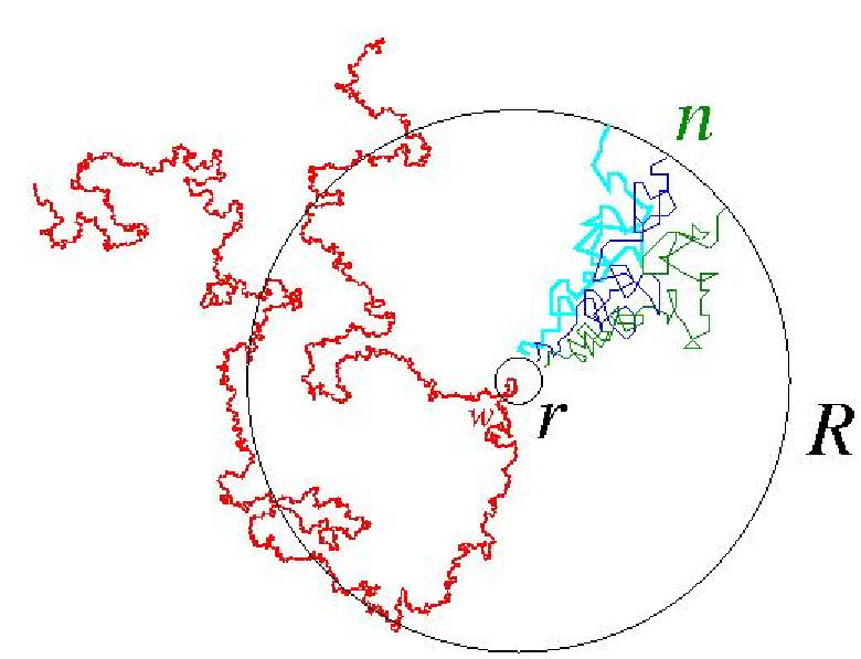
Representation of Moments by Random Walks
By the very definition of the -measure, independent RW’s or Brownian motions diffusing away from the absorber, i.e., from the cluster’s hull’s frontier , and diffusing without hitting , give a geometric representation of the moment in Eq. (6.6) for integer (Fig. 25). Convexity arguments yield the analytic continuation to arbitrary ’s.
Recall the notation for two random sets required to traverse, without mutual intersection, the annulus from the inner boundary circle of radius to the outer one at distance , and for two independent, thus possibly intersecting, sets. With this notation, one can define, as in Eq. (4.3), a grand canonical partition function which describes the star configuration of the Brownian paths and cluster : . At the critical point, it is expected to scale for as
| (6.10) |
where the scaling exponent
| (6.11) |
depends on and is associated with the conformal operator creating the star vertex . The dots after exponent express the fact that there may be an additional contribution to the exponent, independent of , corresponding to the entropy associated with the extremities of the random frontier (see, e.g., Eq. (4.3)).
By normalization, this contribution actually does not appear in the multifractal moments. Since is a probability measure, the sum (6.6) is indeed normalized as
| (6.12) |
or in terms of star partition functions:
| (6.13) |
The scaling behavior (6.10) thus gives
| (6.14) |
The last exponent actually obeys the identity , which will be obtained directly, and can also be seen as a consequence of Gauss’s theorem in two dimensions [71]. Thus we can also write as in (5.2)
| (6.15) |
where is a (grand-canonical) excursion measure from to for the random set , with proper scaling . The factor is the area scaling factor of the annulus .
Proper Scaling Dimensions

In the absence of diffusing Brownian paths, conformally invariant scaling curves possess their own scaling dimensions. Typically, for a single scaling curve, like, e.g., a self-avoiding path, there are three possible environments, corresponding to the neighborhoods of the tip, with scaling dimension , of a point inside the curve (), or of a boundary point (). In these notations, the subscript obviously corresponds to the number of path components attached to the considered point (Fig. 26). Generalizations are given by star exponents and , associated with multiple paths, as in sections 4 or 10.4 below.
The Hausdorff dimension of the curve is related to the scaling dimension in a well-known way:
Quantum Gravity
To calculate exponents, we again use the fundamental mapping between the conformal field theory, describing a critical statistical system in the plane or half-plane , and the same CFT in presence of quantum gravity [56, 58, 57]. Two universal functions and , which now depend on the central charge of the CFT, describe the KPZ map between conformal dimensions in bulk or boundary QG and those in the standard plane or half-plane:
| (6.17) |
with
| (6.18) |
The parameter is the string susceptibility exponent of the random 2D surface (of genus zero), bearing the CFT of central charge [56]; is the solution of
| (6.19) |
In order to simplify the notation, we shall hereafter in this section drop the subscript from functions and .
The function maps quantum gravity conformal weights, whether in the bulk or on a boundary, into their counterparts in or , as in (3.10) (3.12). The function has been tailored to map quantum gravity boundary dimensions to the corresponding conformal dimensions in the full plane , as in (3.63) (3.64). The positive inverse function of , , is
| (6.20) |
and transforms the conformal weights of a conformal operator in or into the conformal weights of the same operator in quantum gravity, in the bulk or on the boundary.
Boundary Additivity Rule
Consider two arbitrary random sets with boundary scaling exponents ,
in the half-plane with Dirichlet boundary conditions. When these two sets are mutually-avoiding, the scaling exponent in , as in (6.11), or in have the universal structure [84, 85, 90]
| (6.21) | |||||
| (6.22) |
We have seen these fundamental relations in the case above; they are established for the general case in Ref. [1]. is, on the random disk with Dirichlet boundary conditions, the boundary scaling dimension corresponding to in the half-plane , and in Eqs. (6.21) (6.22)
| (6.23) |
is a linear boundary exponent corresponding to the fusion of two “boundary operators” on the random disk, under the Dirichlet mutual avoidance condition . This quantum boundary conformal dimension is mapped back by to the scaling dimension in , or by to the boundary scaling dimension in [90].
Exponent Construction


We first need the boundary (conformal) scaling dimension (b.s.d.) associated with the presence of the random frontier near the Dirichlet boundary . Since this frontier is simple, it can be seen as made of two non-intersecting semi-infinite strands (Fig. 27). Its b.s.d. in quantum gravity thus obeys (6.23)
| (6.24) |
where is the boundary scaling dimension of a semi-infinite frontier path originating at the boundary of .
As before, the packet of independent Brownian paths has a boundary scaling dimension
From (6.23) the QG boundary dimension of the whole set is (see Fig. 28):
| (6.25) |
Its associated QG bulk conformal dimension is therefore . From Eqs. (6.18) or (6.21) we finally find
| (6.26) | |||||
The whole construction is illustrated in Fig. 28.
The value of the QG b.s.d. of a simple semi-infinite random path is
| (6.27) |
It is derived in section 10.2 below from the exponents of the model, or of the SLE. It can be directly derived from Makarov’s theorem:
| (6.28) |
which, applied to (6.26), leads to the same result. We thus finally get
| (6.29) |
This result satisfies the identity: , which is related to Gauss’s theorem, as mentioned above.
Multifractal Exponents
The multifractal exponents (6.16) are obtained from (6.17-6.20) as [90]
| (6.30) | |||||
Similar exponents, but associated with moments taken at the tip, later appeared in the context of the process (see II in Ref. [96], and [207]; see also [208] for Laplacian random walks.) The whole family will be given in section 10.6.
The Legendre transform is easily performed to yield:
| (6.31) | |||||
| (6.32) | |||||
It is convenient to express the results in terms of the central charge with the help of:
| (6.33) |
We finally find the
Multifractal Exponents
| (6.34) | |||||
| (6.35) | |||||
Multifractal Spectrum
| (6.36) | |||||
| (6.37) | |||||
Other Multifractal Exponents
This formalism immediately allows generalizations. For instance, in place of a packet of independent random walks, one can consider a packet of independent self-avoiding walks , which avoid the fractal boundary. The associated multifractal exponents are given by (6.29), with the argument in simply replaced by [84]. These exponents govern the universal multifractal behavior of the moments of the probability that a SAW escapes from . One then gets a spectrum such that
thus unveiling
the same invariant
underlying wedge distribution as the harmonic measure (see also [89]).
6.3 Geometrical Analysis of Multifractal Spectra
Makarov’s Theorem
An Invariance Property of
It is interesting to note that the general multifractal function (6.37) can also be written as
| (6.39) |
Thus the multifractal function possesses the invariance symmetry
| (6.40) |
for and satisfying the duality relation:
| (6.41) |
or, equivalently When associating an equivalent electrostatic wedge angle to each local singularity exponent , one gets the complementary rule for angles in the plane
| (6.42) |
Notice that by definition of the multifractal dimension , is the total harmonic measure content of points of type or equivalent angle along the multifractal frontier. The symmetry (6.40) thus means that this harmonic content is invariant when taken at the complementary angle in the plane . The basic symmetry (6.40) thus reflects that of the external frontier itself under the exchange of interior and exterior domains.
Equivalent Wedge Distribution
The geometrical multifractal distribution of wedges along the boundary takes the form:
| (6.44) |
Remarkably enough, the second term also describes the contribution by a wedge to the density of electromagnetic modes in a cavity [209]. The simple shift in (6.44), , from the case to general values of , can then be related to results of conformal invariance in a wedge [210]. The partition function for the two sides of a wedge of angle and size , in a CFT of central charge , indeed scales as [211]
| (6.45) |
Thus, one can view the dependance of result (6.44) as follows: the number of sites, , with local wedge angle along a random path with central charge , is the same as the number of sites, , with wedge angle along a self-avoiding walk (), renormalized by the partition function representing the presence of a -CFT along such wedges:
Hausdorff Dimension of the External Perimeter
The maximum of corresponds to , and gives the Hausdorff dimension of the support of the measure, i.e., the accessible or external perimeter as:
| (6.46) | |||||
| (6.47) |
This corresponds to a typical sigularity exponent
| (6.48) |
and to a typical wedge angle
| (6.49) |
Probability Densities
The probability to find a singularity exponent or, equivalently, to find an equivalent opening angle along the frontier is
| (6.50) |
Using the values found above, one can recast this probability as (see also [89])
| (6.51) |
where
Universal Multifractal Data


The multifractal exponents (Fig. 29) or the generalized dimensions (Fig. 30) appear quite similar for various values of , and a numerical simulation would hardly distinguish the different universality classes, while the functions, as we see in Fig. 31, do distinguish these classes, especially for negative , i.e. large . In Figure 31 we display the multifractal functions , Eq. (6.37), corresponding to various values of , or, equivalently, to a number of components , and in the or Potts models (see below).

Needles
The singularity at , or , in the multifractal functions , or , corresponds to boundary points with a needle local geometry, and Beurling’s theorem [212] indeed insures that the Hölder exponents are bounded below by . This corresponds to large values of , where, asymptotically, for any universality class,
| (6.52) |
Fjords
The right branch of has a linear asymptote
| (6.53) |
The behavior corresponds to moments of lowest order , where reaches its maximal value: , common to all simply connected, conformally-invariant, boundaries. Its linear shape is quite reminiscent of that of the multifractal function of the growth probability as in the case of a 2D DLA cluster [213]. This describes almost inaccessible sites: Define as the number of boundary sites having a given probability to be hit by a RW starting at infinity; the MF formalism yields, for a power law behavior
| (6.54) |
with an exponent
| (6.55) |
RW’s, SAW’s and Percolation
Brownian paths, scaling self-avoiding walks and critical percolation clusters all correspond to CFT’s with , for which we find
| (6.56) | |||||
| (6.57) | |||||
| (6.58) |
where we recognize in particular the percolation exponents (5.10, 5.11). We thus have the general result:
In two dimensions, the harmonic multifractal exponents and spectra of a random walk, a critical percolation cluster, and a self-avoiding walk are
identical in the scaling limit.
The external frontier of a Brownian path and the accessible perimeter of a percolation cluster are
identical to a self-avoiding walk in the scaling limit, with Hausdorff dimension
i.e., the Mandelbrot conjecture.
Ising Clusters
A critical Ising cluster () possesses a multifractal spectrum with respect to the harmonic measure:
| (6.59) | |||||
| (6.60) |
with the dimension of the accessible perimeter
| (6.61) |
Potts Clusters, and “Ultimate Norway”
The limit multifractal spectrum is obtained for , which is an upper or lower bound for all ’s, depending on the position of with respect to :
This MF spectrum provides an exact example of a left-sided MF spectrum, with an asymptote (Fig. 31). It corresponds to singular boundaries where , i.e., where the external perimeter is everywhere dominated by “fjords”, with typical angle . It is tempting to call it the “ultimate Norway”.
The frontier of a Potts Fortuin-Kasteleyn cluster, or the provide such an example for this left-handed multifractal spectrum () (see section 9). The MF data are:
| (6.62) | |||||
| (6.63) |
with accessible sites forming a set of Hausdorff dimension
| (6.64) |
which is also the maximal value common to all multifractal generalized dimensions . The external perimeter which bears the electrostatic charge is a non-intersecting simple path. We therefore arrive at the striking conclusion that in the plane, a conformally-invariant scaling curve which is simple has a Hausdorff dimension at most equal to [90]. The corresponding Potts frontier, while still possessing a set of double points of dimension , actually develops a logarithmically growing number of double points [214]. The values of the various Hausdorff dimensions predicted for Potts clusters have been verified in a nice numerical study [214, 194].
7 Higher Multifractal Spectra
It is interesting to note that one can define higher multifractal spectra as those depending on several variables [87]. A first example is given by the double moments of the harmonic measure on both sides of a random path.
7.1 Double-Sided Spectra

Double-Sided Potential
When it is simple, i.e., double point free, a conformally scaling curve can be reached from both sides. Notice, however, that one can also address the case of non-simple random paths, by concentrating on the double-sided potential near cut-points. For a Brownian path for instance, one can consider the subset of pinching or cut-points, of Hausdorff dimension , where the path splits into two non-intersecting parts. The path is then locally accessible from both directions.
Taking Dirichlet boundary conditions on the random curve, one can then consider the joint distribution of potential on both sides, such that the potential scales as
| (7.1) |
when approaching on one side of the scaling curve, while scaling as
| (7.2) |
on the other side (Fig. 32). The multifractal formalism now characterizes subsets of boundary sites with two such Hölder exponents, , by their Hausdorff dimension . The standard one-sided multifractal spectrum is then recovered as the supremum:
| (7.3) |
Equivalent Wedges
As above, one can also define two equivalent “electrostatic” angles from singularity exponents , as and the dimension of the boundary subset with such is then
| (7.4) |
Double Harmonic Moments
As before, instead of considering directly the potential , one can consider equivalently the harmonic measure. Let be the harmonic measure (as seen from “infinity”) of the intersection of and the ball centered at point Let us consider a covering of the path by such balls centered at points forming a discrete subset of .
Define the double moments of the harmonic measure:
| (7.5) |
where and are respectively the harmonic measures on the “left” or “right” sides of the random path.

These moments are represented by two packets of and independent Brownian paths diffusing away from the fractal path (Fig. 33).
They have a multifractal scaling behavior
| (7.6) |
where the exponent now depends on two moment orders . A Hausdorff dimension is given by the double Legendre transform:
| (7.7) | |||||
It yields the dimension of the subset of frontier points , where the potential scales as in Eqs. (7.1-7.2), or where the harmonic content of a ball scales as on one side, and on the other.
One and Two-Sided Cases
In analogy to Eqs. (6.16), (6.26), the exponent is associated with a scaling dimension , calculated in the quantum gravity formalism in a way similar to (6.29) [95, 1]:
| (7.9) |
The two-sided multifractal spectrum is then obtained by a double Legendre transform as [1, 95]
| (7.10) | |||||
| (7.11) |
with a similar symmetric equation for . This doubly multifractal spectrum possesses the desired property
where is (6.37) above. The domain of definition of the doubly multifractal function is independent of and given by
| (7.12) |
in accordance to Eq. (7.10). The domain of definition of distribution is the image of domain (7.12) in -variables:
| (7.13) |
The total electrostatic angle is thus less than ,
which simply accounts for the electrostatic screening of local
wedges by fractal randomness, as expected.
Notice finally that there also exists a single-sided distribution [1]
| (7.14) |
which corresponds to the potential distribution in the vicinity of the tip of a conformally-invariant scaling path, and naturally differs from the usual spectrum, which describes the potential on one side of the scaling path.
Brownian and SAW’s Double Spectra
In the case of a Brownian path or a self-avoiding walk, one obtains [1, 95]
These doubly multifractal spectra thus are different for RW’s and SAW’s. The SAW spectrum corresponds to (7.10) for , and possesses the required property
where is (6.58) above. For a Brownian path, the one-sided spectrum
such that , gives the spectrum of cut-points along the Brownian frontier. This set of Hausdorff dimension is disconnected, and , in contrast to Makarov’s theorem, , for any connected set in the plane.
7.2 Higher Multifractality of Multiple Path Vertices
One can consider a star configuration of a number of similar simple scaling paths, all originating at the same vertex . Higher moments can then be defined by looking at the joint distribution of the harmonic measure contents in each sector between the arms. We shall not describe this general case here, which can be found in full detail in Ref. [1].
8 Winding of Conformally Invariant Curves
Another important question arises concerning the geometry of the equipotential lines near a random (CI) fractal curve. These lines are expected to rotate wildly, or wind, in a spiralling motion that closely follows the boundary itself. The key geometrical object is here the logarithmic spiral, which is conformally invariant (Fig. 34).

The MF description should generalize to a mixed multifractal spectrum, accounting for both scaling and winding of the equipotentials [108].
In this
section, we describe the exact solution to this mixed MF spectrum
for any random CI curve [109]. In particular, it is shown
to be related by a scaling law to the usual
harmonic MF spectrum. We use the same conformal tools as before, fusing quantum
gravity and Coulomb gas methods, which allow the
description of Brownian paths interacting and winding with CI curves,
thereby providing a probabilistic description of the potential map near any CI curve.
With I. A. Binder, we have also obtained recently a rigorous derivation of this spectrum
for the SLE [156].
8.1 Harmonic Measure and Rotations
Consider again a (CI) critical random cluster, or scaling curve, generically called . Let be the potential at an exterior point , with Dirichlet boundary conditions on the outer (simply connected) boundary of , and on a circle “at ”, i.e., of a large radius scaling like the average size of . As we have seen, the potential is identical to the probability that a Brownian path started at escapes to “” without having hit .
Let us now consider the degree with which the curves wind in the complex plane about point and call . In the scaling limit, the multifractal formalism, here generalized to take into account rotations [108], characterizes subsets of boundary sites by a Hölder exponent , and a rotation rate , such that their potential lines respectively scale and logarithmically spiral as
| (8.1) |
in the limit . The Hausdorff dimension defines the mixed MF spectrum, which is CI since under a conformal map both and are locally invariant.
As above, we consider the harmonic measure , which is the integral of the Laplacian of in a disk of radius centered at , i.e., the boundary charge in that disk. It scales as with the same exponent as in (8.1), and is also the probability that a Brownian path started at large distance first hits the boundary at a point inside . Let be the associated winding angle of the path down to distance from . The mixed moments of and , averaged over all realizations of , are defined as
| (8.2) |
where the sum runs over the centers of a covering of the boundary by disks of radius , and where and are real numbers. As before, the moment of is the probability that independent Brownian paths diffuse along the boundary and all first hit it at points inside the disk . The angle is then their common winding angle down to distance (Fig. 35).

8.2 Exact Mixed Multifractal Spectra
The 2D conformally invariant random statistical system is labelled by its central charge , [19]. The main result is the following exact scaling law [109]:
| (8.4) | |||||
where is the usual harmonic MF spectrum in the absence of prescribed winding, first obtained in Ref. [90], and described in section 6, Eq. (6.37). It can be recast as:
| (8.5) | |||||
We thus arrive at the very simple formula for the mixed spectrum:
| (8.6) |
Notice that by conformal symmetry
i.e., the most likely situation in the absence of prescribed rotation is the same as , i.e. winding-free. The domain of definition of the usual (8.2) is [212], thus for -spiralling points Eq. (8.4) gives
| (8.7) |
We have seen in section 6.3 the geometrical meaning to the exponent : For an angle with opening , , and the quantity can be regarded as a local generalized angle with respect to the harmonic measure. The geometrical MF spectrum of the boundary subset with such opening angle and spiralling rate reads from (8.6)
As in (8.7), the domain of definition in the variable is
The maximum is reached when the two frontier strands about point locally collapse into a single -spiral, whose inner opening angle is [212].
In the absence of prescribed winding (), the maximum gives the dimension of the external perimeter of the fractal cluster, which is a simple curve without double points, and may differ from the full hull [90, 86]. Its dimension (6.47) reads in this notation
It corresponds to typical values and
For spirals, the maximum value still corresponds in the Legendre transform (8.3) to , and gives the dimension of the subset of the external perimeter made of logarithmic spirals of type . Owing to (8.4) we immediately get
| (8.8) |
This corresponds to typical scaled values
Since and , the EP dimension decreases with spiralling rate, in a simple parabolic way.


Fig. 36 displays typical multifractal functions . The example choosen, , corresponds to the cases of a SAW, or of a percolation EP, the scaling limits of which both coincide with the Brownian frontier [84, 85, 88]. The original singularity at in the rotation free MF functions , which describes boundary points with a needle local geometry, is shifted for towards the minimal value (8.7). The right branch of has a linear asymptote Thus the -curves all become parallel for , i.e., , corresponding to deep fjords where winding is easiest.
Limit multifractal spectra are obtained for , which exhibit examples of left-sided spectra, with a horizontal asymptote (Fig. 37). This corresponds to the frontier of a Potts cluster (i.e., the ), a universal random scaling curve, with the maximum value , and a vanishing typical opening angle , i.e., the “ultimate Norway” where the EP is dominated by “fjords” everywhere [90, 95].
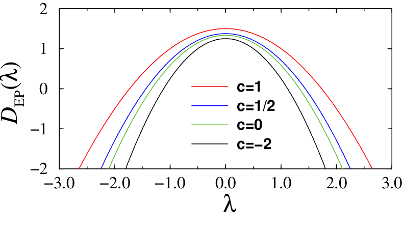
Fig. 38 displays the dimension as a function of the rotation rate , for various values of , corresponding to different statistical systems. Again, the case shows the least decay with , as expected from the predominence of fjords there.
8.3 Conformal Invariance and Quantum Gravity
We now give the main lines of the derivation of exponents , hence [109]. As usual, independent Brownian paths , starting a small distance away from a point on the frontier , and diffusing without hitting , give a geometric representation of the moment, , of the harmonic measure in Eq. (8.2) for integer (Fig. 35), extended by convexity to arbitrary ’s. Let us introduce an abstract (conformal) field operator characterizing the presence of a vertex where such Brownian paths and the cluster’s frontier diffuse away from each other in the mutually-avoiding configuration [84, 85]; to this operator is associated a scaling dimension . To measure rotations using the moments (8.2) we have to consider expectation values with insertion of the mixed operator
| (8.9) |
where is the winding angle common to the frontier and to the Brownian paths (see Fig. (35)), and where is the scaling dimension of the operator . It is directly related to by
| (8.10) |
For , one recovers the previous scaling dimension
As in section 6, we use the fundamental KPZ mapping of the CFT in the plane to the CFT on a random Riemann surface, i.e., in presence of 2D quantum gravity [56], and the universal functions and , acting on conformal weights, which describe the map:
| (8.11) |
with . As before, the parameter is the solution of
For the purely harmonic exponents , describing the mutually-avoiding set , we have seen in Eqs. (6.29) and (6.24) that
| (8.12) |
where is the positive inverse of ,
In (8.12), we recall that the arguments and are respectively the boundary scaling dimensions (b.s.d.) (6.24) of the simple path representing a semi-infinite random frontier (such that ), and of the packet of Brownian paths, both diffusing into the upper half-plane . The function transforms these half-plane b.s.d’s into the corresponding b.s.d.’s in quantum gravity, the linear combination of which gives, still in QG, the b.s.d. of the mutually-avoiding set . The function finally maps the latter b.s.d. into the scaling dimension in . The path b.s.d. (6.24) obeys .
It is now useful to consider semi-infinite random paths , joined at a single vertex in a mutually-avoiding star configuration . (In this notation the frontier near any of its points is a two-star .) The scaling dimension of can be obtained from the same b.s.d. additivity rule in quantum gravity, as in (6.21) or (8.12) [90]
| (8.13) |
The scaling dimensions (8.12) and (8.13) coincide when
| (8.14) | |||||
| (8.15) |
Thus we state the scaling star-equivalence
| (8.16) |
of two mutually-avoiding simple paths , further avoiding Brownian motions, to simple paths in a mutually-avoiding star configuration (Fig. 39). This equivalence plays an essential role in the computation of the complete rotation spectrum (8.9).

8.4 Rotation Scaling Exponents
The Gaussian distribution of the winding angle about the extremity of a scaling path, like , was derived in Ref. [34], using exact Coulomb gas methods. The argument can be generalized to the winding angle of a star about its center [215], where one finds that the angular variance is reduced by a factor (see also [216]). The scaling dimension associated with the rotation scaling operator is found by analytic continuation of the Fourier transforms evaluated there [109]:
i.e., is given by a quadratic shift in the star scaling exponent. To calculate the scaling dimension (8.10), it is sufficient to use the star-equivalence (8.15) above to conclude that
which is the key to our problem. Using Eqs. (8.15), (8.12), and (8.11) gives the useful identity:
with . Recalling (8.10), we arrive at the multifractal result:
| (8.17) |
where corresponds to the purely harmonic spectrum with no prescribed rotation.
8.5 Legendre Transform
The structure of the full -function (8.17) leads by a formal Legendre transform (8.3) directly to the identity
where , with , is the purely harmonic MF function. It depends on the natural reduced variable à la Beurling ()
whose expression emerges explicitly from (8.12). Whence Eq.(8.4), QED.
It is interesting to consider also higher multifractal spectra [95]. For a conformally-invariant scaling curve which is simple, i.e., without double points, like the external frontier , here taken alone, define the universal function which gives the Hausdorff dimension of the points where the potential varies jointly with distance as on one side of the curve, and as on the other, given a winding at rate . This function is
| (8.18) | |||||
and satisfies the generalization of scaling relation (8.4)
| (8.19) |
9 & Potts Models and the Stochastic Löwner Evolution
9.1 Geometric Duality in and Potts Cluster Frontiers
Model
The model partition function is that of a gas of self- and mutually-avoiding loops on a given lattice, e.g., the hexagonal lattice [24]:
| (9.1) |
where and are two fugacities, associated respectively with the total number of occupied bonds , and with the total number of loops , i.e., polygons drawn on the lattice. For , this model possesses a critical point (CP), , while the whole “low-temperature” (low-) phase, i.e., , has critical universal properties, where the loops are denser than those at the critical point [24].
Potts Model
The partition function of the -state Potts model [217] on, e.g., the square lattice, with a second order critical point for , has a Fortuin-Kasteleyn (FK) representation at the CP [218]: where the configurations are those of unions of FK clusters on the square lattice, with a total number of polygons encircling all clusters, and filling the medial square lattice of the original lattice [23, 24]. Thus the critical Potts model becomes a dense loop model, with loop fugacity , while one can show that its tricritical point with site dilution [25] corresponds to the CP [77, 198]. The geometrical clusters, made of like spins in the (critical) Potts model, have been argued to also correspond to the tricritical branch of the Potts model with dilution, [219]. Their frontiers are then the critical loops of the corresponding model with the same central charge, in agreement with RefS. [77, 198].
Coulomb Gas
The and Potts models thus possess the same “Coulomb gas” representations [23, 24, 77, 198]:
with for the CP or tricritical Potts model, and for the low- or critical Potts models; the coupling constant of the Coulomb gas also yields the central charge:
| (9.2) |
Notice that from the expression (6.19) of in terms of one arrives at the simple relation:
| (9.3) |
The above representation for gives a range of values ; our results also apply for , corresponding, e.g., to the branch, with a low- phase for , and CP for
Hausdorff Dimensions of Hull Subsets
The fractal dimension of the accessible perimeter, Eq. (6.47), is, like , a symmetric function of and once rewritten in terms of :
| (9.4) |
where is the Heaviside distribution. Thus is given by two different analytic expressions on either side of the separatrix . The dimension of the full hull, i.e., the complete set of outer boundary sites of a cluster, has been determined for and Potts clusters [32], and is
| (9.5) |
for the entire range of the coupling constant . Comparing to Eq. (9.4), we therefore see that the accessible perimeter and hull Hausdorff dimensions coincide for , i.e., at the CP (or for tricritical Potts clusters), whereas they differ, namely , for , i.e., in the low- phase, or for critical Potts clusters. This is the generalization to any Potts model of the effect originally found in percolation [92]. This can be directly understood in terms of the singly connected sites (or bonds) where fjords close in the scaling limit. Their dimension is given by [32]
| (9.6) |
For critical loops, , so that hence there exist no closing fjords, thereby explaining the identity:
| (9.7) |
In contrast, one has and for critical Potts
clusters and for the low- phase. In this case, pinching points of
positive dimension appear in the scaling limit,
so that (Table 1).
| 0 | 1 | 2 | 3 | 4 | |
|---|---|---|---|---|---|
| -2 | 0 | 1/2 | 4/5 | 1 | |
Duality
We then find from Eq. (9.4), with :
| (9.8) |
The symmetry point corresponds to , , or , where, as expected, the dimension of the pinching points vanishes.
For percolation, described either by , or by the low- model with , we recover the result , recently derived in Ref. [86]. For the Ising model, described either by , or by the CP with , we observe that the EP dimension coincides, as expected, with that of critical loops, which in fact appear as EP’s. This is a particular case of a further duality relation between the critical Potts and CP models:
| (9.9) |
In terms of this duality, the central charge takes the simple expression:
| (9.10) |
Exactly the same duality exists between the frontiers of Potts FK and geometrical clusters, as studied in Ref. [219].
9.2 Geometric Duality of
Stochastic Löwner Evolution

An introduction to the stochastic Löwner evolution process () can be found in Refs. [4], [207], [3]. Here we consider the so-called chordal SLE in the complex half-plane. A similar definition of radial SLE exists for the complex plane.
The trace of this process is a conformally-invariant random path in the half-plane . The Riemann conformal map , from the slit half-plane to itself, obeys the stochastic Löwner equation [93]
where is a one-dimensional Brownian motion on the real line , with diffusion constant The map is normalized (“hydrodynamic” normalization) and the curve parameterized with respect to time (half-plane capacity parametrization), so that has the asymptotic behavior at infinity:
for all .
The random path can be a simple or a non-simple path with self-contacts. The is parameterized by , which describes the rate of the auxiliary Brownian motion along the boundary, which is the source for the process. When , the random curve is simple, while for , the curve is a self-coiling path [105]. For the path is space filling.
The trace of this SLE process essentially describes the boundaries of (Potts) clusters or hulls we have introduced above, or the random lines of the model. The correspondence to the previous parameters, the central charge , the string susceptibility exponent , or the Coulomb gas constant , is as follows.
In the original work by Schramm [93], the variance of the Gaussian winding angle of the single extremity of a of size was calculated, and found to be
In [34] we found, for instance for the extremity of a random line in the model, the corresponding angular variance
from which we immediately infer the identity
| (9.11) |
The low-temperature branch of the model, for , indeed corresponds to and describes non-simple curves, while corresponds to . The critical point branch gives , while gives . The range probably corresponds to higher multicritical points with . Owing to Eq. (9.3) for , we have
| (9.12) | |||||
| (9.13) |
Duality
The central charge (6.19) or (9.2) is accordingly:
| (9.14) |
an expression which of course is symmetric under the duality , or
| (9.15) |
reflecting the symmetry under [90]. The self-dual form of the central charge is accordingly:
| (9.16) |
From Eqs. (9.5) and (9.4) we respectively find [90]
| (9.17) |
| (9.18) |
the first result being later derived rigorously in probability theory [105, 107].
For , we have . For , the self-coiling scaling paths obey the duality equation (9.8) derived above, recast here in the context of the process:
| (9.19) |
where now
Thus we predict that the external perimeter of a self-coiling process is, by duality, the simple path of the process.
The symmetric point corresponds to the model, or Potts model, with . The value corresponds to a self-avoiding walk, which thus appears [85, 86] as the external frontier of a process, namely that of a percolation hull [93, 98].
Let us now study more of the ’s random geometry using the quantum gravity method described here.
Up to now, we have described general conformally-invariant curves in the plane in terms of the universal parameters (central charge) or (string susceptibility). The multifractal results described in the sections above thus apply to the after substituting for or . Care should be taken, however, in such a substitution since two dual values of (9.15) correspond to a same value of . The reason is that up to now we have considered boundary geometrical properties which actually were self-dual. An exemple is the harmonic multifractal spectrum of the frontier, which is identical to that of the smoother (simple) path. So we actually saw only the set of simple SLE traces with . When dealing with higher multifractality, we assumed the random curves to be simple. When dealing with non-simple random paths, boundary quantum gravity rules are to be modified as explained now.
10 Quantum Gravity Duality and SLE
10.1 Dual Dimensions
It will be convenient to introduce the following notations. The standard KPZ map reads:
| (10.1) |
where is a planar conformal dimension and its quantum gravity counterpart, and where we recall that is the negative root of
| (10.2) |
We introduce the dual quantum dimension of , such that:
| (10.3) |
and
| (10.4) |
Similarly, let us define the variable , dual of susceptibility exponent , by:
| (10.5) |
which is simply the (“non-physical”) positive root of Eq. (10.2):
| (10.6) |
The dual equation of (10.3) is then:
| (10.7) |
By construction we have the simultaneous equations:
| (10.8) |
with the positive solution
| (10.9) |
We define a dual KPZ map by the same equation as (10.1), with substituted for . It has the following properties1515 15 It generalizes to any operator the so-called “wrong” KPZ gravitational dressing of the boundary identity operator [60].:
| (10.10) | |||||
| (10.11) | |||||
| (10.12) |
Boundary KPZ for Non Simple Paths
The additivity rules in quantum gravity for the boundary scaling dimensions of mutually-avoiding random paths and are:
| (10.13) | |||||
| (10.14) |
For simple paths, like random lines in the model at its critical point, or the SLE trace for the boundary dimensions are additive in quantum gravity, a fundamental fact repeatedly used above. On the other hand, for non-simple paths, the dual dimensions are additive in boundary quantum gravity. This is the case of random lines in the dense phase of the model, or, equivalently, of hulls of Fortuin-Kasteleyn clusters in the Potts model, or of the trace. These additivity rules are derived from the consideration of partition functions on a random surface in the dilute or dense phases. (See [1], Appendices B & C.)
The composition rules for non-simple paths are different from the ones for simple paths, when written in terms of the standard string susceptibility exponent , but they are formally identical in terms of the dual exponent .
Bulk KPZ for Non-Simple Paths
For determining the complete set of scaling dimensions, it remains to relate bulk and boundary dimensions. In the dilute phase, i.e., for simple paths, we have seen the simple relation in a random metric (see Appendix C in Ref. [1]):
| (10.15) |
The KPZ map from boundary dimension in quantum gravity to bulk dimension in the plane reads accordingly
| (10.16) |
where
| (10.17) |
an expression repeatedly used above. When dealing with non-simple paths, these relations have to be changed to:
| (10.18) |
as shown in detail in Ref. [1]. At this stage, the reader will not be surprised that this relation is just identical to the dual of (10.15)
| (10.19) |
when now written in terms of both dual dimensions and susceptibility exponent. As a consequence, the scaling dimension of a bulk operator in a dense system reads:
| (10.20) |
which by duality can necessarily be written as:
| (10.21) | |||||
as can be easily checked. This QG duality is analyzed in greater detail in Ref. [1].
In summary, the composition rules for scaling dimensions, whether on a boundary or in the bulk, take a unique analytic form for both phases (simple or non-simple paths), provided one replaces the string susceptibility exponent in the simple case by its dual variable in the non-simple case, and QG dimensions by their duals. This applies to the dense phase of the model, or to Potts cluster boundaries, and in particular to .
10.2 KPZ for SLE
QG Duality for SLE
The QG duality is perfectly adapted to the parametrization of the process. Indeed we have from (9.12) and (9.13)
| (10.22) | |||||
| (10.23) |
so that the analytical forms of and its dual are simply exchanged when passing from simple paths () to non-simple ones (). Because of the equivalent dual equations (10.10), by choosing either the -solution or the -solution, depending whether or , we can write
| (10.24) |
with now a single function, valid for all values of parameter
| (10.25) |
Similarly, the inverse KPZ map (10.9) reads, according to (10.11) or (10.12):
| (10.26) |
again with a single expression of the inverse function, valid for any
| (10.27) |
I emphasize that coincides with the KPZ map for , while it represents the dual of the latter when and then acts on the dual dimension . For instance, we have the important result at the origin
| (10.28) |
which vanishes for simple paths, and is non-trivial for non-simple ones.
Composition Rules for SLE
Finally we can conclude with general composition rules for the SLE process. Indeed, the boundary rule in (10.13) or its dual (10.14), owing to Eqs. (10.24) and (10.26), read in a unified way in terms of parameter :
| (10.33) |
valid for the entire range of . Similarly, the composition rules for SLE’s in the plane are found from Eqs. (10.15) or (10.19), and recast according to (10.2) and (10.26) into a unified formula, valid for any
| (10.34) |
Thus we see that by introducing dual equations we have been able to unify the composition rules for the SLE in a unique way, which no longer depends explicitly on the range of .
10.3 Short Distance Expansion

Boundary SDE
Consider the power law governing the behavior of two mutually-avoiding random paths and anchored at the Dirichlet boundary line, and approaching each other at short distance along the line. The probability of such an event scales like
| (10.35) |
where the short-distance exponent reads [19, 28]:
| (10.36) |
We simply use the fusion rule (10.33) and the quadratic map (10.25) to immediately get
| (10.37) |
where we use as a short-hand notation. In terms of quantum gravity boundary dimensions, or their dual, this SDE exponent splits into
So we see that the short-distance expansion (SDE) along the boundary of is governed by the product of the quantum boundary dimensions, or of their duals, depending on the phase we are in. In particular, if one chooses the set to be the chordal SLE trace itself, its boundary dimension is such that in the dilute phase, or in the dense phase. That corresponds to the single expression , which is for or for . In this case, the expressions (10.37) or (10.3) simplify to
| (10.41) | |||||
The boundary contact exponent between an SLE and an arbitrary conformally invariant scaling set in the standard (half-) plane is therefore identical with the purely gravitational boundary exponent of the set !
In a way, in the standard plane, the local randomness of the SLE acts exactly as quantum gravity for approaching scaling sets like , when the latter have to avoid the SLE.
This explains the observation made in Ref. [110] that the boundary SDE of any operator with the SLE trace might be seen as exhibiting (boundary) quantum gravity. However, we see that if for the SDE exponent (10.41) is indeed the KPZ solution , for it necessarily transforms to the dual dimension introduced above in (10.3) . The appearance of the simple quantum gravity dimension results from the consideration of the SDE with a boundary SLE, since the general structure of SDE exponent (10.3) is clearly still quadratic and given by the product of quantum gravity dimensions or their dual.
Bulk SDE
One can also consider the SDE for random paths in the full plane, corresponding to the so-called radial SLE. Consider the power law governing the behavior of two mutually-avoiding random paths and approaching each other at short distance in the plane, with probability
| (10.45) |
where the short-distance exponent now reads:
| (10.46) |
In the case where the set is chosen to be the radial SLE trace itself, taken at a typical medial point, the expression simplify into
So the SDE of the SLE trace with any operator in the plane again generates the boundary dimension of in quantum gravity or its dual, modulo a constant shift. Notice that this shift is self-dual with respect to and reads also .
10.4 Multiple Paths in , Potts Models and SLE

Let us consider the scaling dimensions associated with several (mutually-avoiding) random paths starting from a same small neighborhood, also called star exponents in the above (Figure 42). It is simpler to first give them for the model, before transferring them to the SLE. These exponents can be derived explicitly from the quantum gravity approach, in particular in presence of a boundary (see Appendix B in Ref. [1]). (See also refs. [58, 59, 61, 120].)
Multiple SLE’s in QG
Near the boundary of a random surface with Dirichlet conditions, the conformal dimensions read
| (10.50) |
where the “” superscript stands for the dense phase. The quantum bulk dimensions read similarly
| (10.51) |
The dilute phase corresponds to (9.12) for , while the dense one covers (9.13) with :
| (10.52) | |||||
| (10.53) |
By using dual dimensions (10.3) for the dense phase, these results are unified into
| (10.54) | |||||
| (10.55) | |||||
| (10.56) | |||||
| (10.57) |
Hence we observe that in the dense phase the dual dimensions play the role of the original ones in the dilute phase.
Multiple SLE’s in and
The scaling dimensions in the standard complex half-plane , or in the complex plane , can now be obtained from the quantum gravity ones by the KPZ -map (10.1), or, in the SLE formalism, from the (10.24) or (10.2) adapted KPZ maps. From the last equations (10.54) to (10.57), it is clear that by duality the analytic form of the dimensions stays the same in the two phases , and . Indeed we get:
| (10.58) | |||||
| (10.59) | |||||
| (10.60) | |||||
| (10.61) |
10.5 and Quantum Gravity

An extension of the original SLE, the stochastic process, has been introduced in Ref. [112] (see also [115, 116, 117, 118]). A drift term of strength is added to the boundary Brownian process that appears in the Löwner equation driving the uniformizing Riemann map of the trace. For , one recovers the usual SLE process: As a consequence, the chordal feels an asymmetrical “pressure” that tends to push it away from one side of the Dirichlet boundary (Figure 43).
As shown in Ref. [115], the is completely equivalent, in terms of conformal properties or critical exponents, to a standard in the presence, on the same side of the boundary, of a packet of independent Brownian paths which are avoided by the trace, and exert a “conformal pressure” (Fig. 43). The value of is given by the formula
| (10.62) |
We can then use the QG formalism to give yet another representation of the process and give a simple meaning to parameter (10.62). The equivalent Brownian packet associated with the process can indeed be replaced by multiple SLE’s. Multiple s and a Brownian packet are conformally equivalent if and only if their boundary QG dimensions (for ), or their dual boundary QG dimensions (for ), coincide:
both cases yield naturally the same anaytical result. Therefore the parameter simply appears as the number of equivalent multiple ’s avoided by the original one (Fig. 43) (See also [118].)
Contact Exponents for

One can use this QG conformal equivalence to predict other properties of the composite process.
A first question is that of the minimal value of the drift or pressure parameter such that the trace of completely avoids the negative part of the half-plane boundary. For , the trace of always avoids , while for it always bounces onto it. The minimal value of simply corresponds to a minimal number of equivalent Brownian paths, whence:
| (10.63) |
where we used (10.28). As expected, this minimal value for [116] is non vanishing only for .
Consider also the probability that a packet of independent Brownian paths avoids a chordal , while starting at distance from it on the boundary (Fig. 44). This probability scales as , and the contact exponent can be calculated with the help of the Brownian equivalence and of the contact exponent (10.41) for standard SLE (see figures 43 and 41). One finds
where is given by . Again a contact exponent, , acting in the standard (half-) plane, actually is a quantum gravity exponent! (Fig. 44).
10.6 Multifractal Exponents for Multiple SLE’s
In section 6 above we have studied in detail the multifractal spectrum associated with the harmonic measure near a conformally-invariant frontier, generalized to the mixed rotation spectrum in section 8. We also looked at the double-sided distribution of potential near a simple fractal curve. We have seen in previous sections 10.1 and 10.2 how to extend the formalism to non-simple curves, by using duality. We now briefly apply it to some other spectra associated with the harmonic measure near multiple paths. They include the so-called SLE derivative exponents [96].
Boundary Multifractal Exponents
Let us start with geometrical properties of CI curves near the boundary of (chordal SLE). We specifically look at the scaling behavior of moments of the harmonic measure, or in SLE terms, of powers (of the modulus of) the derivative of the Riemann map that maps the SLE trace back to the half-line [96, 207, 3].
Consider the -leg boundary operator creating a star made of semi-infinite random paths , diffusing in the upper half-plane and started at a single vertex on the real line in a mutually-avoiding star configuration as seen in section 10.4 (Fig 42). Its boundary scaling dimension is given by Eqs. (10.58) or (10.60):
| (10.64) |
with the inversion formula:
| (10.65) |
We thus dress this -star by a packet of independent Brownian paths diffusing away from the apex of the star, located on the boundary, while avoiding the star’s paths (Fig. 45).

Boundary Derivative Exponents
It is interesting to isolate in these exponents the contribution (10.64) coming from the SLE paths, and define a subtracted exponent, the (boundary) derivative exponent [96], which is obtained after simplication as
For , one recovers the result of Ref. [96]. The linear structure so obtained is in agreement with the short-distance expansion results (10.37) and (10.3); mutual-avoidance between SLE and Brownian paths enhances the independent path exponent by times a typical boundary QG term.
Boundary Disconnection Exponents
Notice that for the exponent is not necessarily trivial:
So this exponent takes non-zero values for , i.e. for self-coiling CI curves. This is typical of a disconnection exponent: Consider a point located along the boundary at short distance from the origin where all paths of the SLE star are started. The probability that point stays connected to infinity without being encircled by the collection of SLE traces scales like
If , the probability that the SLE paths return to the boundary is zero, and any point stays connected to infinity, hence a vanishing disconnection exponent .
Planar Multifractal Exponents
Let us consider now the scaling exponent associated with the moment of the harmonic measure near the tip of a collection of radial SLE paths in the plane. It suffices to use the bulk general composition formula (10.34) in place of the boundary one (10.33) in (10.66) above, to immediately get:
It is useful to separate the contribution of the tip of star
and define a bulk derivative exponent
which generalizes the case considered in Ref. [96].
Planar Disconnection Exponents
For this yields the set of disconnection exponents
which governs the probability that a point , located at distance from the star’s tip , stays connected to infinity without being encircled by the collection of SLE traces:
Here again, it strongly depends on whether the random paths are simple or not, respectively for and . If , the SLE paths are simple curves that cannot encircle any exterior point; the latter therefore stays connected to infinity, hence a vanishing disconnection exponent.
Double-Sided Exponents
Let us mention that boundary double-sided exponents can be defined, corresponding to double moments of the harmonic measure on both sides of a multiple SLE trace, or, equivalently, to double-sided derivative exponents [96, 1]. We have in mind configurations where two packets of and Brownian paths diffuse on both sides of a boundary star . They are easily computed at level from the QG method, and the interested reader is referred to [1].
Winding of Multiple SLE’s
Let us finally return to the winding angle variance at points where strands come together in a star configuration . We have seen in section 8 that the variance of paths up to distance is reduced by a factor with respect to the single path case, namely:
In the case of non-simple paths (), one can further consider the winding at points where strands meet together, amongst which adjacent pairs (with ) are conditioned not to hit each other [216]. In each pair the two strands, which otherwise would bounce on each other, are disconnected from each other, and that corresponds, in our notations, to a star configuration:
| (10.69) |
Wieland and Wilson made the interesting conjecture that in this case the winding angle variance grows like [216]
| (10.70) |
This can be derived from the quantum gravity formalism as follows. A generalization of Eq. (8.15) gives the number of paths, , which is equivalent to strands in a star configuration (10.69), as
Indeed, one simply has to gauge the extra (quantum gravity) conformal weight , associated with the disconnected pairs, by the (QG) boundary conformal weight of a single path extremity. Because of the value (10.28) and the value (10.65) we find
which gives a variance
which is just the conjecture (10.70), QED.
Acknowledgements
It is a pleasure to thank Michael Aizenman for his collaboration on path-crossing exponents in percolation (section 5), after a seminal discussion together with Bob Langlands, and for many enjoyable and fruitful discussions over time; Amnon Aharony for the same shared collaboration; Ilia A. Binder for his collaboration on the mixed multifractal rotation spectrum in section 8; Peter Jones and Benoît Mandelbrot for invitations to the Department of Mathematics at Yale University and to the Mittag-Leffler Institute, and many stimulating discussions; François David for precious help with his Lectures; Emmanuel Guitter for generously preparing the figures; Jean-Marc Luck for extensive help with LaTeX; Bernard Nienhuis and Vincent Pasquier for friendly and interesting discussions; David A. Kosower for a careful reading of the manuscript; Ivan K. Kostov for our early collaboration and intensive discussions; Ugo Moschella for friendly help while preparing the file; and Thomas C. Halsey for many “multifractal” discussions over time, and a careful reading of the manuscript.
Last but not least, Anton Bovier, François Dunlop, Frank den Hollander and Aernout van Enter are especially thanked for having organized this successful Les Houches Session LXXXIII in such a friendly and efficient way, and for their care in editing this volume.
References
- [1] B. Duplantier, Conformal Fractal Geometry & Boundary Quantum Gravity, in: Fractal Geometry and Applications: A Jubilee of Benoît Mandelbrot (M. L. Lapidus and M. van Frankenhuysen, eds.), Proc. Symposia Pure Math. vol. 72, Part 2, 365-482 (AMS, Providence, R.I., 2004), arXiv:math-ph/0303034.
- [2] W. Werner, Some Recent Aspects of Conformally Invariant Systems, in: Les Houches Summer School LXIII Mathematical Statistical Physics, July 4 - 29, 2005, this volume, arXiv:math.PR/0511268.
- [3] W. Werner, Lecture Notes from the 2002 Saint-Flour Summer School, Springer, L. N. Math. 1840, 107-195, (2004), arXiv:math.PR/0303354.
- [4] G. F. Lawler, Conformally Invariant Processes in the Plane, Mathematical Surveys and Monographs, AMS, Vol. 114 (2005).
- [5] M. Bauer and D. Bernard, 2D growth processes: SLE and Loewner chains, Phys. Rep., to appear, arXimath-ph/0602049.
- [6] J. Cardy, SLE for Theoretical Physicists, Ann. Physics 318, 81-118 (2005), cond-mat/0503313.
- [7] W. Kager and B. Nienhuis, J. Stat. Phys. 115, 1149-1229 (2004), arXiv:math-ph/0312056.
- [8] B. Duplantier, Brownian Motion, “Diverse and Undulating”, in: Einstein, 1905-2005, Poincaré Seminar 2005, Eds. T. Damour, O. Darrigol, B. Duplantier and V. Rivasseau (Birkhaüser Verlag, Basel, 2006).
- [9] P. Lévy, Processus stochastiques et mouvement brownien (Gauthier-Villars, Paris, 1965).
- [10] B. B. Mandelbrot, The Fractal Geometry of Nature (Freeman, New-York, 1982).
- [11] K. Symanzyk, in Local Quantum Theory, edited by R. Jost (Academic Press, London, New-York, 1969).
- [12] P.-G. de Gennes, Phys. Lett. A38, 339-340 (1972).
- [13] J. des Cloizeaux and G. Jannink, Polymers in Solution, their Modeling and Structure (Clarendon, Oxford, 1989).
- [14] M. Aizenman, Phys. Rev. Lett. 47, 1-4, 886 (1981); Commun. Math. Phys. 86, 1-48 (1982); D. C. Brydges, J. Fröhlich, and T. Spencer, Commun. Math. Phys. 83, 123-150 (1982).
- [15] G. F. Lawler, Commun. Math. Phys. 86, 539-554 (1982); Intersection of Random Walks (Birkhäuser, Boston, 1991).
- [16] M. E. Fisher, J. Stat. Phys. 34, 667-729 (1984).
- [17] M. Aizenman, Commun. Math. Phys. 97, 91-110 (1985); G. Felder and J. Fröhlich, ibid., 111-124; G. F. Lawler, ibid., 583-594.
- [18] B. Duplantier, Commun. Math. Phys. 117, 279-329 (1987).
- [19] A. A. Belavin, A. M. Polyakov and A. B. Zamolodchikov, Nucl. Phys. B241, 333-380 (1984).
- [20] D. Friedan, J. Qiu, and S. Shenker, Phys. Rev. Lett. 52, 1575-1578 (1984).
- [21] J. L. Cardy, in Phase Transitions and Critical Phenomena, edited by C. Domb and J. L. Lebowitz, (Academic Press, London, 1987), Vol. 11.
- [22] B. Nienhuis, A.N. Berker, E.K. Riedel and M. Schick, Phys. Rev. Lett. 43, 737 (1979).
- [23] M. den Nijs, J. Phys. A 12, 1857-1868 (1979); Phys. Rev. B 27, 1674-1679 (1983).
- [24] B. Nienhuis, Phys. Rev. Lett. 49, 1062-1065 (1982); J. Stat. Phys. 34, 731-761 (1984); in Phase Transitions and Critical Phenomena, edited by C. Domb and J. L. Lebowitz, (Academic Press, London, 1987), Vol. 11.
- [25] B. Nienhuis, J. Phys. A 15, 199-213 (1982).
- [26] J. L. Cardy, Nucl. Phys. B240 [FS12], 514-532 (1984).
- [27] H. Saleur, J. Phys. A 19, L807-L810 (1986); ibid. 20, 455-470 (1987).
- [28] B. Duplantier, Phys. Rev. Lett. 57, 941-944, 2332 (1986); J. Stat. Phys. 54, 581-680 (1989); [see also L. Schäfer, C. von Ferber, U. Lehr, and B. Duplantier, Nucl. Phys. B374, 473-495 (1992)].
- [29] B. Duplantier and H. Saleur, Phys. Rev. Lett. 57, 3179-3182 (1986).
- [30] B. Duplantier, J. Phys. A 19, L1009-L1014 (1986).
- [31] B. Duplantier and H. Saleur, Nucl. Phys. B290 [FS20], 291-326 (1987).
- [32] H. Saleur and B. Duplantier, Phys. Rev. Lett. 58, 2325-2328 (1987).
- [33] B. Duplantier and H. Saleur, Phys. Rev. Lett. 59, 539-542 (1987).
- [34] B. Duplantier and H. Saleur, Phys. Rev. Lett. 60, 2343-2346 (1988).
- [35] J. L. Cardy, J. Phys. A 21, L797-L799 (1988); ibid. 31, L105-L110 (1998) [see also M. Aizenman, Nucl. Phys. B485 [FS], 551-582 (1997)]; ibid. 47, L665-L672 (2001); J. L. Cardy and H. Saleur, J. Phys. A 22, L601-L604 (1989); J. L. Cardy and R. M. Ziff, J. Stat. Phys. 110, 1-33 (2003).
- [36] M. T. Batchelor and H. W. J. Blöte, Phys. Rev. Lett. 61, 138-140 (1988); 1042 (1988).
- [37] M. T. Batchelor, B. Nienhuis, and S. O. Warnaar, Phys. Rev. Lett. 62, 2425-2428 (1989).
- [38] B. Nienhuis, Int. J. Mod. Phys. B4, 929-942 (1990).
- [39] S. O. Warnaar, M. T. Batchelor and B. Nienhuis, J. Phys. A 25, 3077-3095 (1992).
- [40] B. Nienhuis, S. O. Warnaar and H. W. J. Blöte, J. Phys. A 26, 477-493 (1993).
- [41] S. O. Warnaar, B. Nienhuis and K. A. Seaton, Phys. Rev. Lett. 69, 710 (1992).
- [42] V. V. Bazhanov, B. Nienhuis and S. O. Warnaar, Phys. Lett. B. 322, 198-206 (1994).
- [43] J. L. Cardy, J. Phys. A 25, L201-L206 (1992).
- [44] H. Saleur, Nucl. Phys. B382, 486-531 (1992), arXiv:hep-th/9111007.
- [45] M. T. Batchelor, J. Suzuki, and C. M. Yung, Phys. Rev. Lett. 73, 2646-2649 (1994); M. T. Batchelor and C. M. Yung, Phys. Rev. Lett. 74, 2026-2029 (1995); J. Phys. A 28 L421-L426 (1995), arXiv:cond-mat/9507010; Nucl. Phys. B453, 552-580 (1995), arXiv:hep-th/9506074.
- [46] J. Kondev, J.C. de Gier and B. Nienhuis, J. Phys. A 29, 6489 (1996).
- [47] B. Nienhuis, Physica A 251, 104-114 (1998).
- [48] J. L. Jacobsen and J. Kondev, Phys. Rev. Lett. 81, 2922-2925 (1998), arXiv:cond-mat/9805178; Nucl. Phys. B532, 635-688 (1998), arXiv:cond-mat/9804048; J. Stat. Phys. 96, 21-48 (1999), arXiv:cond-mat/9811085.
- [49] V. S. Dotsenko, J. L. Jacobsen, and M. Picco, Nucl. Phys. B618, 523-550 (2001), arXiv:hep-th/0105287.
- [50] J. L. Jacobsen, N. Read, and H. Saleur, Phys. Rev. Lett. 90, 090601 (2003).
- [51] J. L. Jacobsen and J. Kondev, Phys. Rev. Lett. 92, 210601 (2004), arXiv:cond-mat/0401504.
- [52] R. Langlands, P. Pouliot, and Y. Saint-Aubin, Bull. Amer. Math. Soc. 30, 1-61 (1994).
- [53] M. Aizenman, in Mathematics of Multiscale Materials; the IMA Volumes in Mathematics and its Applications, K. M. Golden et al. eds, Springer-Verlag (1998).
- [54] I. Benjamini and O. Schramm, Commun. Math. Phys. 197, 75-107 (1998).
- [55] V. A. Kazakov, Phys. Lett. A119, 140-144 (1986).
- [56] A. M. Polyakov, Mod. Phys. Lett. A 2, 893-898 (1987); V. G. Knizhnik, A. M. Polyakov and A. B. Zamolodchikov, Mod. Phys. Lett. A 3, 819-826 (1988).
- [57] F. David, Mod. Phys. Lett. A 3, 1651-1656 (1988); J. Distler and H. Kawai, Nucl. Phys. B321, 509-527 (1988).
- [58] B. Duplantier and I. K. Kostov, Phys. Rev. Lett. 61, 1433-1436 (1988); Nucl. Phys. B340, 491-541 (1990).
- [59] I. K. Kostov, Mod. Phys. Lett. A 4, 217-226 (1989); M. Gaudin and I. K. Kostov, Phys. Lett. B220, 200-206 (1989); I. K. Kostov, Nucl. Phys. B376, 539-598 (1992), arXiv:hep-th/9112059.
- [60] I. K. Kostov and M. Staudacher, Nucl. Phys. B384, 459-483 (1992), arXiv:hep-th/9203030.
- [61] V. Kazakov and I. K. Kostov, Nucl. Phys. B386, 520-557 (1992), arXiv:hep-th/9205059.
- [62] B. B. Mandelbrot, J. Fluid. Mech. 62, 331-358 (1974).
- [63] H. G. E. Hentschel and I. Procaccia, Physica D 8, 435-444 (1983).
- [64] U. Frisch and G. Parisi, in Proceedings of the International School of Physics “Enrico Fermi”, course LXXXVIII, edited by M. Ghil (North-Holland, New York, 1985) p. 84.
- [65] T. C. Halsey, M. H. Jensen, L. P. Kadanoff, I. Procaccia, and B. I. Shraiman, Phys. Rev. A 33, 1141-1151 (1986); ibid. 34, 1601 (1986).
- [66] M. Cates and J. M. Deutsch, Phys. Rev. A 35, 4907-4910 (1987); B. Duplantier and A. Ludwig, Phys. Rev. Lett. 66, 247-251 (1991); C. von Ferber, Nucl. Phys. B490, 511-542 (1997).
- [67] T. C. Halsey, P. Meakin, and I. Procaccia, Phys. Rev. Lett. 56, 854-857 (1986).
- [68] T. C. Halsey, Multifractality, Scaling, and Diffusive Growth in Fractals: Physical Origin and Properties, L. Pietronero, ed. (Plenum Publishing Co., New York, 1989).
- [69] P. Meakin, Fractals, Scaling and Growth Far from Equilibrium, Cambridge Nonlinear Sc. Series 5 (1999).
- [70] B. B. Mandelbrot and C. J. G.. Evertsz, Nature 348, 143-145 (1990); C. J. G. Evertsz and B. B. Mandelbrot, Physica A 177, 589-592 (1991).
- [71] M. E. Cates and T. A. Witten, Phys. Rev. Lett. 56, 2497-2500 (1986); Phys. Rev. A 35, 1809-1824 (1987).
- [72] G. F. Lawler, The frontier of a Brownian path is multifractal, preprint (1998).
- [73] B. Duplantier and K.-H. Kwon, Phys. Rev. Lett. 61, 2514-2517 (1988).
- [74] B. Li and A. D. Sokal, J. Stat. Phys. 61, 723-748 (1990); E. E. Puckette and W. Werner, Elect. Commun. in Probab. 1, 49-64 (1996).
- [75] K. Burdzy and G. F. Lawler, Probab. Th. Rel. Fields 84, 393-410 (1990); Ann. Probab. 18, 981-1009 (1990).
- [76] G. F. Lawler, Duke Math. J. 47, 655-694 (1980); 53, 249-270 (1986).
- [77] B. Duplantier, J. Stat. Phys. 49, 411-431 (1987); B. Duplantier and F. David, J. Stat. Phys. 51, 327-434 (1988).
- [78] S. Majumdar, Phys. Rev. Lett. 68, 2329-2331 (1992); B. Duplantier, Physica A 191, 516-522 (1992).
- [79] R. W. Kenyon, Acta Math. 185, 239-286 (2000).
- [80] R. W. Kenyon, J. Math. Phys. 41, 1338-1363 (2000).
- [81] W. Werner, Probab. Th. Rel. Fields 108, 131-152 (1997).
- [82] G. F. Lawler and W. Werner, Ann. Probab. 27, 1601-1642 (1999).
- [83] B. Duplantier, Phys. Rev. Lett. 81, 5489-5492 (1998).
- [84] B. Duplantier, Phys. Rev. Lett. 82, 880-883 (1999), arXiv:cond-mat/9812439.
- [85] B. Duplantier, Phys. Rev. Lett. 82, 3940-3943 (1999), arXiv:cond-mat/9901008.
- [86] M. Aizenman, B. Duplantier and A. Aharony, Phys. Rev. Lett. 83, 1359-1362 (1999), arXiv:cond-mat/9901018 .
- [87] B. Duplantier, in Fractals: Theory and Applications in Engineering, M. Dekking et al. eds., pp. 185-206 (Springer-Verlag, 1999).
- [88] G. F. Lawler and W. Werner, J. European Math. Soc. 2, 291-328 (2000).
- [89] J. L. Cardy, J. Phys. A 32, L177-L182 (1999), arXiv:cond-mat/9812416.
- [90] B. Duplantier, Phys. Rev. Lett. 84, 1363-1367 (2000), arXiv:cond-mat/9908314.
- [91] P. Di Francesco, O. Golinelli, and E. Guitter, Nucl. Phys. B570, 699-712 (2000), arxiv:cond-mat/9910453; P. Di Francesco, E. Guitter, and J. L. Jacobsen, Nucl. Phys. B580, 757-795 (2000), arXiv:cond-mat/0003008.
- [92] T. Grossman and A. Aharony, J. Phys. A 19, L745-L751 (1986); ibid. 20, L1193-L1201 (1987).
- [93] O. Schramm, Israel Jour. Math. 118, 221-288 (2000).
- [94] For the identification of to LERW, Schramm mentions that he used the Gaussian winding result found by R. Kenyon for spanning trees and LERW [79, 80]. The earlier general formula found in Ref. [34] was actually immediately giving the SLE parameter in terms of the Coulomb gas constant , hence for the model, .
- [95] B. Duplantier, J. Stat. Phys. 110, 691-738 (2003), arXiv:cond-mat/0207743.
- [96] G. F. Lawler, O. Schramm, and W. Werner, Acta Math. 187, (I) 237-273, (II) 275-308 (2001), arXiv:math.PR/9911084, arXiv:math.PR/0003156; Ann. Inst. Henri Poincaré PR 38, 109-123 (2002), arXiv:math.PR/0005294.
- [97] G. F. Lawler, O. Schramm, and W. Werner, Acta Math. 189, 179-201 (2002), arXiv:math.PR/0005295; Math. Res. Lett. 8, 401-411 (2001), math.PR/0010165.
- [98] S. Smirnov, C. R. Acad. Sci. Paris Sér. I Math. 333, 239-244 (2001).
- [99] G. F. Lawler, O. Schramm, and W. Werner, Electronic J. of Probability 7, 2002, paper no.2, arXiv:math.PR/0108211.
- [100] S. Smirnov and W. Werner, Math. Res. Lett. 8, 729-744 (2001), arXiv:math.PR/0109120.
- [101] G. F. Lawler, O. Schramm, and W. Werner, Ann. Probab. 32, 939-995 (2004), arXiv:math.PR/0112234.
- [102] G. F. Lawler, O. Schramm, and W. Werner, On the Scaling limit of Planar Self-Avoiding Walks, in: Fractal Geometry and Applications: A Jubilee of Benoît Mandelbrot (M. L. Lapidus and M. van Frankenhuysen, eds.), Proc. Symposia Pure Math. vol. 72, Part 2, 339-364 (AMS, Providence, R.I., 2004), arXiv:math.PR/0204277.
- [103] T. G. Kennedy, Phys. Rev. Lett. 88, 130601 (2002).
- [104] The duality prediction follows immediately from the duality results of [90], and the correspondence between the SLE parameter and the Coulomb gas constant .
- [105] S. Rohde and O. Schramm, Ann. Math. 161, 879-920 (2005), arXiv:math.PR/0106036.
- [106] V. Beffara, Ann. Probab. 32, 2606-2629 (2004), arXiv:math.PR/0204208; see also V. Beffara and V. Sidoravicius, Percolation Theory, in: Encyclopedia of Mathematical Physics (Elsevier, Amsterdam, 2006), arXiv:math.PR/0507220.
- [107] V. Beffara, The Dimension of the SLE Curves, arXiv:math.PR/0211322.
- [108] I. A. Binder, Harmonic Measure and Rotation of Simply Connected Planar Domains, PhD Thesis, Caltech (1997).
- [109] B. Duplantier and I. A. Binder, Phys. Rev. Lett. 89, 264101 (2002); arXiv:cond-mat/0208045.
- [110] M. Bauer and D. Bernard, Phys. Lett. B543, 135-138 (2002), arXiv:math-ph/0206028; Commun. Math. Phys. 239, 493-521 (2003), arXiv:hep-th/0210015; Phys. Lett. B557, 309-316 (2003), arXiv:hep-th/0301064; Ann. Henri Poincaré 5, 289-326 (2004), arXiv:math-ph/0305061; Phys. Lett. B583, 324-330 (2004), arXiv:math-ph/0310032; Proceedings of the conference Conformal Invariance and Random Spatial Processes, Edinburgh, July 2003, arXiv:math-ph/0401019.
- [111] M. Bauer, D. Bernard, J. Houdayer, J. Stat. Mech. P03001 (2004), arXiv:math-ph/0411038.
- [112] G. F. Lawler, O. Schramm, and W. Werner, J. Amer. Math. Soc. 16, 917-955 (2003), arXiv:math.PR/0209343.
- [113] R. Friedrich and W. Werner, C. R. Acad. Sci. Paris Sér. I Math. 335, 947-952 (2002), arXiv:math.PR/0209382; Commun. Math. Phys., 243, 105-122 (2003), arXiv:math-ph/0301018.
- [114] R. Friedrich, On Connections of Conformal Field Theory and Stochastic Lœwner Evolution, arXiv:math-ph/0410029.
- [115] W. Werner, Ann. Fac. Sci. Toulouse, 13, 121-147 (2004), arXiv:math.PR/0302115.
- [116] J. Dubédat, Ann. Probab. 33, 223-243 (2005), arXiv:math.PR/0303128.
- [117] J. Cardy, and Conformal Field Theory, arXiv:math-ph/0412033.
- [118] K. Kytölä, On Conformal Field Theory of , arXiv:math-ph/0504057.
- [119] R. O. Bauer, R. M. Friedrich, Diffusing polygons and SLE(), arXiv:math.PR/0506062.
- [120] J. L. Cardy, J. Phys. A 36, L379-L386 (2003); erratum J. Phys. A 36, 12343 (2003), arXiv:math-ph/0301039; Phys. Lett. B582, 121-126 (2004), arXiv:hep-th/0310291.
- [121] J. Dubédat, Commutation Relations for SLE, arXiv:math.PR/0411299.
- [122] J. Dubédat, Euler Integrals for Commuting SLEs, arXiv:math.PR/0507276.
- [123] M. Bauer, D. Bernard, K. Kytölä, J. Stat. Phys. 120, 1125-1163 (2005), arXiv:math-ph/0503024.
- [124] G. M. T. Watts, J. Phys. A 29, L363-L368 (1996).
- [125] J. Dubédat, Excursion Decompositions for SLE and Watts’ Crossing Formula, arXiv:math.PR/0405074.
- [126] J. Dubédat, Commun. Math. Phys. 245, 627-637 (2004), arXiv:math.PR/0306056.
- [127] F. Camia and C. M. Newman, Continuum Nonsimple Loops and 2D Critical Percolation, arXiv:math.PR/0308122.
- [128] F. Camia and C. M. Newman, The Full Scaling Limit of Two-Dimensional Critical Percolation, arXiv:math.PR/0504036.
- [129] F. Camia, L. R. G. Fontes and C. M. Newman, The Scaling Limit Geometry of Near-Critical 2D Percolation, arXiv:cond-mat/0510740.
- [130] V. Beffara, Cardy’s Formula on the Triangular Lattice, the Easy Way, Preprint, http://www.umpa.ens-lyon.fr/ vbeffara/files/Proceedings-Toronto.pdf (2005).
- [131] V. Beffara, Critical Percolation on Other Lattices, Talk at the Fields Institute, http://www.fields.utoronto.ca/audio/05-06/ (2005).
- [132] D. Bernard, G. Boffetta, A. Celani and G. Falkovich, Nature Physics 2, 124-128 (2006).
- [133] G. Kozma, Scaling limit of loop-erased random walk - a naive approach, arXiv:math.PR/0212338.
- [134] O. Schramm and S. Sheffield, Ann. Probab. 33, 2127-2148 (2005), arXiv:math.PR/0310210.
- [135] S. Smirnov, in preparation (2006).
- [136] G. F. Lawler and W. Werner, Probab. Th. Rel. Fields 128, 565-588 (2004), arXiv:math.PR/0304419.
- [137] W. Werner, Conformal Restriction and Related Questions, Proceedings of the conference Conformal Invariance and Random Spatial Processes, Edinburgh, July 2003, Probability Surveys 2, 145-190 (2005), arXiv:math.PR/0307353.
- [138] W. Werner, C. R. Acad. Sci. Paris Sér. I Math. 337, 481-486 (2003), arXiv:math.PR/0308164.
- [139] S. Sheffield and W. Werner, in preparation (2006).
- [140] M. Konsevich, CFT, SLE and Phase Boundaries, Preprint of the Max Planck Institute (Arbeitstagung 2003), 2003-60a.
- [141] R. Friedrich and J. Kalkkinen, Nucl. Phys. B687, 279-302 (2004), arXiv:hep-th/0308020.
- [142] D. Zhan, Probab. Theory Related Fields 129, 340-380 (2004), arXiv:math.PR/0310350.
- [143] R. O. Bauer and R. M. Friedrich, C. R. Math. Acad. Sci. Paris 339, 579-584 (2004), arXiv:math.PR/0408157; On radial stochastic Loewner evolution in multiply connected domains, arXiv:math.PR/0412060; On Chordal and Bilateral SLE in multiply connected domains, arXiv:math.PR/0503178.
- [144] B. Doyon, V. Riva and J. Cardy, Identification of the stress-energy tensor through conformal restriction in SLE and related processes, arXiv:math-ph/0511054.
- [145] J. Cardy, J. Phys. A 34, L665-672 (2001), arXiv:cond-mat/0107223.
- [146] C. Richard, A. J. Guttmann and I. Jensen, J. Phys. A 34, L495-501 (2001), arXiv:cond-mat/0107329.
- [147] J. Cardy, Phys. Rev. Lett. 72, 1580-1583 (1994).
- [148] J. Cardy and R. Ziff, J. Stat. Phys. 101, 1-33 (2003), arXiv:cond-mat/0205404.
- [149] C. Garban and J. A. Trujillo Ferreras, The expected area of the filled planar Brownian loop is , arXiv:math.PR/0504496.
- [150] C. Richard, J. Phys. A 37, 4493-4500 (2004), arXiv:cond-mat/0311346.
- [151] W. Werner, The Conformally Invariant Measure on Self-Avoiding Loops, arXiv:math.PR/0511605.
- [152] S. Sheffield, Gaussian Free Fields for Mathematicians, arXiv:math.PR/0312099.
- [153] O. Schramm and S. Sheffield, Contour Lines of the 2D Gaussian Free Field, in preparation (2006).
- [154] S. Sheffield, in preparation (2006).
- [155] E. Bettelheim, I. Rushkin, I. A. Gruzberg and P. Wiegmann, Phys. Rev. Lett. 95, 170602 (2005), arXiv:hep-th/0507115.
- [156] I. A. Binder and B. Duplantier, Multifractal Properties of Harmonic Measure and Rotations for Stochastic Loewner Evolution, in preparation (2006).
- [157] D. Beliaev, Harmonic Measure on Random Fractals, PhD thesis, KTH, Stockholm, Sweden (2005).
- [158] V. Fateev, A. B. Zamolodchikov, and Al. Zamolodchikov, arXiv:hep-th/0001012.
- [159] B. Ponsot and J. Techner, Nucl. Phys. B622, 309-327 (2002), arXiv:hep-th/0110244.
- [160] I. K. Kostov, Nucl. Phys. B658, 397-416 (2003), arXiv:hep-th/0212194; Nucl. Phys. B689, 3-36 (2004), arXiv:hep-th/0312301.
- [161] I. K. Kostov, B. Ponsot, and D. Serban, Nucl. Phys. B683, 309-362 (2004), arXiv:hep-th/0307189.
- [162] O. Angel and O. Schramm, Commun. Math. Phys. 241, 191–213 (2003), arXiv:math.PR/0207153.
- [163] O. Angel, Geom. Funct. Anal. 13, 935-974 (2003), arXiv: math.PR/0208123.
- [164] O. Angel Scaling of Percolation on Infinite Planar Maps, I, arXiv:math.PR/0501006.
- [165] G. Schaeffer, Bijective census and random generation of Eulerian planar maps with prescribed vertex degrees, Electron. J. Combin. 4 (1997) # 1; G. Schaeffer, Conjugaison d’arbres et cartes combinatoires aléatoires, PhD Thesis (1998), Université Bordeaux 1.
- [166] M. Bousquet-Mélou and G. Schaeffer, The degree distribution in bipartite planar maps: applications to the Ising model, arXiv:math.CO/0211070.
- [167] Ph. Di Francesco and E. Guitter, Phys. Rep. 415, 1-88 (2005).
- [168] J. Bouttier, Physique statistique des surfaces aléatoires et combinatoire bijective des cartes planaires, PhD Thesis (2005), Université Paris 6.
- [169] W. N. Guo, B. Nienhuis, H. W. J. Blöte, Phys. Rev. Lett. 96, 045704 (2006), arXiv:cond-mat/0511277.
- [170] W. Janke and A. M. J. Schakel, Phys. Rev. Lett. 95, 135702 (2005).
- [171] See, e.g., A. M. Polyakov, Gauge Fields and Strings (Harwood-Academic, Chur, 1987).
- [172] D. V. Boulatov, V. A. Kazakov, I. K. Kostov and A. A. Migdal, Nucl. Phys. B275, 641-686 (1986); F. David, Nucl. Phys. B257, 45-58 (1985); ibid. 543-576; J. Ambjorn, B. Durhuus, and J. Fröhlich, ibid., 433-449.
- [173] E. P. Wigner, Proc. Cambridge Philos. Soc. 47, 790 (1951).
- [174] F. Dyson, J. Math. Phys. 3, 140, 157, 166, 1199 (1962); Commun. Math. Phys. 19, 235 (1970).
- [175] M. L. Mehta and M. Gaudin, Nucl. Phys. A 18, 395 (1960); A 25, 447 (1961).
- [176] F. Dyson and M. L. Mehta, J. Math. Phys. 4, 701, 713 (1963).
- [177] M. L. Mehta, Random Matrices, 2nd edition (Academic Press, New York, 1991).
- [178] G. ’t Hooft, Nucl. Phys. B72, 461 (1974).
- [179] E. Brézin, C. Itzykson, G. Parisi, J.-B. Zuber, Commun. Math. Phys. 59, 35-51 (1978).
- [180] W. T. Tutte, Can. J. Math. 14, 21 (1962).
- [181] É. Brézin and V. A. Kazakov, Phys. Lett. B236 (1990) 144; M. Douglas and S. Shenker, Nucl. Phys. B335 (1990) 635; D. Gross and A. A. Migdal, Phys. Rev. Lett. 64 (1990) 127; Nucl. Phys. B340 (1990) 333.
- [182] F. David, Simplicial Quantum Gravity and Random Lattices, in: Gravitation and Quantizations, in: Les Houches Summer School, Session LVII, July 5 - August 1, 1992 (Elsevier, Amsterdam, 1993).
- [183] F. David, Random Matrices and Two-Dimensional Gravity, in: Fundamental Problems in Statistical Mechanics VIII, Altenberg (Germany), June 28 – July 10, 1993 (Elsevier, Amsterdam, 1994).
- [184] B. Eynard, Random Matrices, Saclay Lectures in Theoretical Physics, SPhT-T01/014 (2001).
- [185] J. Ambjorn, B. Durhuus and T. Jonsson, Quantum Geometry, a Statistical Field Theory Approach, Cambridge Monographs in Mathematical Physics (Cambridge University Press, Cambridge, 1997).
- [186] G. ’t Hooft, Counting Planar Diagrams with Various Restrictions, arXiv:hep-th/9808113.
- [187] Ph. Di Francesco, P. Ginsparg, and J. Zinn-Justin, Phys. Rep. 254, 1-133 (1995).
- [188] I. K. Kostov, Conformal Field Theory Techniques in Random Matrix Models, arXiv:hep-th/9907060.
- [189] I. K. Kostov and M. L. Mehta, Phys. Lett. B189, 118-124 (1987).
- [190] D. Aldous, SIAM J. Disc. Math. 3, 450 (1990); A. Broder, in 30th Annual Symp. Foundations Computer Sci. 442, (IEEE, New York, 1989).
- [191] G. F. Lawler, Israel Jour. Math. 65, 113-132 (1989).
- [192] G. F. Lawler, Elect. Commun. in Probab. 1, 29-47 (1996).
- [193] C. von Ferber and Y. Holovatch, Europhys. Lett. 39, 31-36 (1997); Phys. Rev. E 56, 6370-6386 (1997); ibid. 59, 6914-6923 (1999); ibid. 65, 092801 (2002); Physica A 249, 327-331 (1998).
- [194] J. Asikainen, A. Aharony, B. B. Mandelbrot, E. M. Rauch, J.-P. Hovi, Eur. Phys. J. B 34, 479-487 (2003), arXiv:cond-mat/0212216.
- [195] B. Sapoval, M. Rosso, and J.-F. Gouyet, J. Physique Lett. 46, 149-156 (1985).
- [196] J. L. Jacobsen and P. Zinn-Justin, Phys. Rev. E 66, 055102 (2002), arXiv:cond-mat/0207063.
- [197] J. L. Cardy, Lectures on Conformal Invariance and Percolation, Chuo University, Tokyo (2001), arXiv:math-ph/0103018.
- [198] B. Duplantier, Phys. Rep. 184, 229-257 (1989).
- [199] P. Meakin et al., Phys. Rev. A 34, 3325-3340 (1986); see also: P. Meakin, ibid. 33, 1365-1371 (1986); in Phase Transitions and Critical Phenomena, vol. 12, edited by C. Domb and J.L. Lebowitz (Academic Press, London, 1988).
- [200] P. Meakin and B. Sapoval, Phys. Rev. A 46, 1022-1034 (1992).
- [201] T. C. Halsey and M. Leibig, Ann. Phys. (N.Y.) 219, 109-147 (1992).
- [202] D. S. Grebenkov, M. Filoche, and B. Sapoval, Eur. Phys. J. B 36, 221-231 (2003).
- [203] S. Kakutani, Proc. Acad. Japan. 20, 706-714 (1944).
- [204] N. G. Makarov, Proc. London Math. Soc. 51, 369-384 (1985); see also P. W. Jones and T. H. Wolff, Acta Math. 161, 131-144 (1988); C. J. Bishop and P. W. Jones, Ann. Math. 132, 511-547 (1990).
- [205] M. Aizenman and A. Burchard, Duke Math. J. 99, 419-453 (1999).
- [206] R. C. Ball, B. Duplantier, and T. C. Halsey, unpublished (1999).
- [207] G. F. Lawler, An Introduction to the Stochastic Löwner Evolution, in: Random Walks and Geometry, V. Kaimonovich ed., 263-293 (de Gruyter, Berlin, 2004).
- [208] M. B. Hastings, Phys. Rev. Lett. 88, 055506 (2002).
- [209] R. Balian and B. Duplantier, Ann. Physics 112, 165-208 (1978), p.183.
- [210] B. Duplantier and J. L. Cardy, private discussion (Aspen, 1999).
- [211] J. L. Cardy, Nucl. Phys. B300, 377-392 (1988).
- [212] A. Beurling, The Collected Works of Arne Beurling. Vol. 1, Contemporary Mathematicians, Birkhäuser Boston Inc., Boston, MA, 1989, Complex analysis, edited by L. Carleson et al.
- [213] R. C. Ball and R. Blumenfeld, Phys. Rev. A 44, R828-R831 (1991).
- [214] A. Aharony and J. Asikainen, Fractals 11 (Suppl.), 3-7 (2003), arXiv:cond-mat/0206367.
- [215] B. Duplantier, unpublished.
- [216] B. Wieland and D. B. Wilson, Phys. Rev. E 68, 056101 (2003).
- [217] R. B. Potts, Proc. Camb. Phil. Soc. 48, 106-109 (1952); F. Y. Wu, Rev. Mod. Phys. 54, 235-268 (1982), erratum 55, 315 (1983).
- [218] C. M. Fortuin and P. W. Kasteleyn, Physica 57, 536-564 (1972).
- [219] W. Janke and A. M. J. Schakel, Nucl. Phys. B700, 385 (2004), arXiv:cond-mat/0311624. [See also A. Coniglio and W. Klein, J. Phys. A 13, 2775-2780 (1980); A. L. Stella and C. Vanderzande, Phys. Rev. Lett. 62, 1067-1070 (1989); ibid. 63, 2537; B. Duplantier and H. Saleur, ibid. 63, 2536.]