From Random Matrices to Stochastic OperatorsThanks: Submitted for publication 19 July 2006. Revised 6 September 2006.

Alan Edelman and Brian D. Sutton Address: Alan Edelman
Department of Mathematics
Massachusetts Institute of Technology
Cambridge, MA 02139 Address: Brian D. Sutton
Department of Mathematics
Randolph-Macon College
Ashland, VA 23005

Abstract.

We propose that classical random matrix models are properly viewed as finite difference schemes for stochastic differential operators. Three particular stochastic operators commonly arise, each associated with a familiar class of local eigenvalue behavior. The stochastic Airy operator displays soft edge behavior, associated with the Airy kernel. The stochastic Bessel operator displays hard edge behavior, associated with the Bessel kernel. The article concludes with suggestions for a stochastic sine operator, which would display bulk behavior, associated with the sine kernel.

Key words and phrases:

random matrices, random eigenvalues, stochastic differential operators

1. Introduction

Through a number of carefully chosen, eigenvalue-preserving transformations, we show that the most commonly studied random matrix distributions can be viewed as finite difference schemes for stochastic differential operators. Three operators commonly arise—the stochastic Airy, Bessel, and sine operators—and these operators are associated with three familiar classes of local eigenvalue behavior—soft edge, hard edge, and bulk.

For an example, consider the Hermite, or Gaussian, family of random matrices. Traditionally, a random matrix from this family has been defined as a dense Hermitian matrix with Gaussian entries, but we show that such a matrix is equivalent, via similarity, translation, and scalar multiplication, to a matrix of the form

\frac{1}{h^{2}}\Delta+\diag_{-1}(x_{1},\dots,x_{n-1})+\frac{2}{\sqrt{\beta}}\cdot\text{``noise''},

in which $\Delta$ is the $n$ -by- $n$ second difference matrix, $\diag_{-1}(x_{1},\dots,x_{n-1})$ is an essentially diagonal matrix of grid points, and the remaining term is a random bidiagonal matrix of “pure noise.” We claim that this matrix encodes a finite difference scheme for

-\frac{d^{2}}{dx^{2}}+x+\frac{2}{\sqrt{\beta}}\cdot\text{``noise''},

which is the inspiration for the stochastic Airy operator. (The “noise” term will be made precise later.)

The idea of interpreting the classical ensembles of random matrix theory as finite difference schemes for stochastic differential operators was originally presented in July 2003 [3], and the theory was developed in [16]. The present article contains several original contributions, including firm foundations for the stochastic Airy and Bessel operators.

The standard technique for studying local eigenvalue behavior of a random matrix distribution involves the following steps. (1) Choose a family of $n$ -by- $n$ random matrices, $n=2,3,4,\dots$ , (2) Translate and rescale the $n$ th random matrix to focus on a particular region of the spectrum, and (3) Let $n\rightarrow\infty$ . When this procedure is performed carefully, so that the eigenvalues near zero approach limiting distributions as $n\rightarrow\infty$ , the limiting eigenvalue behavior often falls into one of three classes: soft edge, hard edge, or bulk.

The largest eigenvalues of many random matrix distributions, notably the Hermite (i.e., Gaussian) and Laguerre (i.e., Wishart) ensembles, display soft edge behavior. The limiting marginal density, as the size of the matrix approaches infinity, of a single eigenvalue at the soft edge is associated with the Airy kernel. Tracy and Widom derived formulas for these density functions in the cases $\beta=1,2,4$ , relating them to solutions of the Painlevé II differential equation. See Figure 1.1(a). Relevent references include [5, 8, 9, 19, 20, 22, 23].

The smallest eigenvalues of some random matrix distributions, notably the Laguerre and Jacobi ensembles, display hard edge behavior. The limiting marginal density of a single eigenvalue at the hard edge is associated with the Bessel kernel. Formulas exist for these density functions as well, expressible in terms of solutions to Painlevé equations. See Figure 1.1(b). Relevant references include [5, 6, 11, 21].

The eigenvalues in the middle of the spectra of many random matrix distributions display bulk behavior. In this case, the spacing between consecutive eigenvalues is interesting. The spacing distributions are associated with the sine kernel, and formulas for the density functions, due to Jimbo, Miwa, Môri, Sato, Tracy, and Widom, are related to the Painlevé V differential equation. See Figure 1.1(c). Relevant references include [7, 11, 12, 18].

This article contends that the most natural setting for soft edge behavior is in the eigenvalues of the stochastic Airy operator

(1.1)

-\frac{d^{2}}{dx^{2}}+x+\frac{2}{\sqrt{\beta}}\cdot\text{``noise''},

and the most natural setting for hard edge behavior is in the singular values of the stochastic Bessel operator

(1.2)

-2\sqrt{x}\frac{d}{dx}+\frac{a}{\sqrt{x}}+\frac{2}{\sqrt{\beta}}\cdot\text{``noise''}.

A suggestion for a stochastic sine operator, along the lines of (1.1–1.2), is presented at the end of the article. The correct interpretations of the “noise” terms in (1.1) and (1.2) will be specified later in the article, as will boundary conditions; see Definitions 3.2 and 3.4. The parameter $\beta$ has its usual meaning from random matrix theory, but now the cases $\beta=1,2,4$ do not seem special.

Numerical evidence is presented in Figures 1.2 and 1.3. The first compares histograms of stochastic Airy eigenvalues to the soft edge distributions of Figure 1.1(a), and the second compares histograms of stochastic Bessel singular values to the hard edge distributions of Figure 1.1(b). The computations were based on the Rayleigh-Ritz method. They are explained in further detail in Sections 7.1 and 7.2.

The stochastic Airy, Bessel, and sine operators were discovered by interpreting the classical ensembles of random matrix theory as finite difference schemes. We argue that

(1)

When scaled at the soft edge, the Hermite and Laguerre matrix models encode finite difference schemes for the stochastic Airy operator.
(2)

When scaled at the hard edge, the Laguerre and Jacobi matrix models encode finite difference schemes for the stochastic Bessel operator.

See Section 3.2 for an overview. Exactly what is meant by “scaling” will be developed later in the article. Typically, scaling involves subtracting a multiple of an identity matrix and multiplying by a scalar to focus on a particular region of the spectrum, along with a few tricks to decompose the matrix into a random part and a nonrandom part. The structured matrix models introduced by Dumitriu and Edelman [1] and further developed by Killip and Nenciu [10] and Edelman and Sutton [4] play vital roles.

The original contributions of this article include the following.

•

The stochastic Airy and Bessel operators are defined. Care is taken to ensure that the operators involve ordinary derivatives of well behaved functions, avoiding any heavy machinery from functional analysis.
•

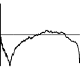
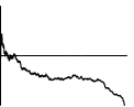
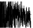
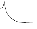
The smoothness of eigenfunctions and singular functions is investigated. In the case of the stochastic Airy operator, the $k$ th eigenfunction is of the form $f_{k}\phi$ , in which $f_{k}$ is twice differentiable and $\phi$ is a once differentiable (specifically $C^{3/2-}$ ) function defined by an explicit formula. This predicts structure in the eigenvectors of certain rescaled matrix models, which can be seen numerically in Figure 1.4. Figure 1.5 considers analogous results for the stochastic Bessel operator.
•

The interpretation of random matrix models as finite difference schemes for stochastic differential operators is developed. This approach is demonstrated for the soft edge of Hermite, the soft and hard edges of Laguerre, and the hard edge of Jacobi.

eigenvector of $H_{\text{soft}}^{\beta}$	$\log\|v\|$	$\nabla\log\|v\|$	$\nabla^{2}\log\|v\|$
first	once differentiable	continuous
second	once differentiable	continuous
${\displaystyle\frac{\text{second}}{\text{first}}}$	twice differentiable	once differentiable	continuous

right singular vector of $J_{\text{hard}}^{\beta,a,b}$	$\log\|v\|$	$\nabla\log\|v\|$
first	continuous
second	continuous
${\displaystyle\frac{\text{second}}{\text{first}}}$	once differentiable	continuous

Notable work of others includes [2] and [14]. Although the stochastic Airy operator is not explictly mentioned in the large $\beta$ asymptotics of Dumitriu and Edelman [2], it appears to play an important role. The stochastic operator approach has very recently been given a boost by Ramírez, Rider, and Virág [14], who have proved a conjecture contained in [3, 16] relating the eigenvalues of the stochastic Airy operator to soft edge behavior. In addition, they have used the stochastic Airy operator to describe the soft edge distributions in terms of a diffusion process.

The next section reviews necessary background material and introduces notation. Section 3 provides formal definitions for the stochastic Airy and Bessel operators and provides an overview of our results, which are developed in later sections.

2. Background

Much work in the field of random matrix theory can be divided into two classes: global eigenvalue behavior and local eigenvalue behavior.

Global eigenvalue behavior refers to the overall density of eigenvalues along the real line. For example, a commonly studied distribution on $n$ -by- $n$ Hermitian matrices known as the Hermite ensemble typically has a high density of eigenvalues near zero, but just a scattering near $\sqrt{2n}$ by comparison. Such a statement does not describe how the eigenvalues are arranged with respect to each other in either region, however.

In contrast, local eigenvalue behavior is observed by “zooming in” on a particular region of the spectrum. The statistic of concern may be the marginal distribution of a single eigenvalue or the distance between two consecutive eigenvalues, for example. Local eigenvalue behavior is determined by two factors—the distribution of the random matrix and the region of the spectrum under consideration. For example, the eigenvalues of the Hermite ensemble near zero display very different behavior from the eigenvalues near the edge of the spectrum, at $\sqrt{2n}$ . Conceivably, the eigenvalues of a different random matrix may display entirely different behavior.

Interestingly, though, the eigenvalues of many, many random matrix distributions fall into one of three classes of behavior, locally speaking. Notably, the eigenvalues of the three classical ensembles of random matrix theory—Hermite, Laguerre, and Jacobi—fall into these three classes as the size of the matrix approaches infinity.

In this section, we present background material, covering the three most commonly studied random matrix distributions and the three classes of local eigenvalue behavior.

2.1. Random matrix models

There are three classical distributions of random matrix theory: Hermite, Laguerre, and Jacobi. The distributions are also called ensembles or matrix models. They are defined in this section. Also, joint distributions for Hermite eigenvalues, Laguerre singular values, and Jacobi CS values are provided. We use the word spectrum to refer to all eigenvalues or singular values or CS values, depending on context. Also, note that the language earlier in the article was loose, referring to eigenvalues when it would have been more appropriate to say “eigenvalues or singular values or CS values.”

2.1.1. Hermite

The Hermite ensembles also go by the name of the Gaussian ensembles. Traditionally, three flavors have been studied, one for real symmetric matrices, one for complex Hermitian matrices, and one for quaternion self-dual matrices. In all three cases, the density function is

(2.1)

\text{const}\times\exp\left(-\frac{\beta}{2}\tr A^{2}\right)dA,

in which $\beta=1$ for the real symmetric case, $\beta=2$ for the complex Hermitian case, and $\beta=4$ for the quaternion self-dual case. The entries in the upper triangular part of such a matrix are independent Gaussians, although the diagonal and off-diagonal entries have different variances.

The eigenvalues of the Hermite ensembles have joint density

(2.2)

\text{const}\times e^{-\frac{\beta}{2}\sum_{i=1}^{n}\lambda_{i}^{2}}\prod_{1\leq i<j\leq n}|\lambda_{i}-\lambda_{j}|^{\beta}\prod_{i=1}^{n}d\lambda_{i}.

Dumitriu and Edelman extended the Hermite ensembles to all $\beta>0$ [1]. Below, $X\sim Y$ indicates that $X$ and $Y$ have the same distribution.

Definition 2.1.

The $n$ -by- $n$ $\beta$ -Hermite matrix model is the random real symmetric matrix

H^{\beta}\sim\frac{1}{\sqrt{2\beta}}\left[\begin{array}[]{ccccc}\sqrt{2}G_{1}&\chi_{(n-1)\beta}\\ \chi_{(n-1)\beta}&\sqrt{2}G_{2}&\chi_{(n-2)\beta}\\ &\ddots&\ddots&\ddots\\ &&\chi_{2\beta}&\sqrt{2}G_{n-1}&\chi_{\beta}\\ &&&\chi_{\beta}&\sqrt{2}G_{n}\end{array}\right],

in which $G_{1},\dots,G_{n}$ are standard Gaussian random variables, $\chi_{r}$ denotes a chi-distributed random variable with $r$ degrees of freedom, and all entries in the upper triangular part are independent.

The $\beta=1,2$ cases can be derived by running a tridiagonalization algorithm on a dense random matrix with density function (2.1), a fact first observed by Trotter [24]. $H^{\beta}$ is the natural extension to general $\beta$ , and it has the desired eigenvalue distribution.

Theorem 2.2 ([1]).

For all $\beta>0$ , the eigenvalues of the $\beta$ -Hermite matrix model have joint density (2.2).

As $\beta\rightarrow\infty$ , the $\beta$ -Hermite matrix model converges in distribution to

H^{\infty}=\frac{1}{\sqrt{2}}\left[\begin{array}[]{cccccc}0&\sqrt{n-1}\\ \sqrt{n-1}&0&\sqrt{n-2}\\ &\sqrt{n-2}&0&\sqrt{n-3}\\ &&\ddots&\ddots&\ddots\\ &&&\sqrt{2}&0&\sqrt{1}\\ &&&&\sqrt{1}&0\end{array}\right].

This matrix encodes the recurrence relation for Hermite polynomials. In fact, the eigenvalues of this matrix are the roots of the $n$ th polynomial, and the eigenvectors can be expressed easily in terms of the first $n-1$ polynomials. See [16] and [17] for details.

2.1.2. Laguerre

The Laguerre ensembles are closely related to Wishart matrices from multivariate statistics. Just like the Hermite ensembles, the Laguerre ensembles come in three flavors. The $\beta=1$ flavor is a distribution on real $m$ -by- $n$ matrices. These matrices need not be square, much less symmetric. The $\beta=2$ flavor is for complex matrices, and the $\beta=4$ flavor is for quaternion matrices. In all cases, the density function is

(2.3)

\text{const}\times\exp\left(-\frac{\beta}{2}\tr A^{*}A\right)dA,

in which $A^{*}$ denotes the conjugate transpose of $A$ .

For a Laguerre matrix with $m$ rows and $n$ columns, let $a=m-n$ . It is well known that the singular values of this matrix are described by the density

(2.4)

\text{const}\times e^{-\frac{\beta}{2}\sum_{i=1}^{n}\lambda_{i}}\prod_{i=1}^{n}\lambda_{i}^{\frac{\beta}{2}(a+1)-1}\prod_{1\leq i<j\leq n}|\lambda_{i}-\lambda_{j}|^{\beta}\prod_{i=1}^{n}d\lambda_{i},

in which $\lambda_{i}$ is the square of the $i$ th singular value. As usual, $\beta=1$ for real entries and $\beta=2$ for complex entries.

Dumitriu and Edelman also extended this family of random matrix distributions to all $\beta>0$ and nonintegral $a$ . The notation in this article differs from the original notation, instead following [16].

Definition 2.3.

The $n$ -by- $n$ $\beta$ -Laguerre matrix model, parameterized by $a>-1$ , is the distribution on real symmetric matrices

L^{\beta,a}\sim\frac{1}{\sqrt{\beta}}\left[\begin{array}[]{ccccc}\chi_{(a+n)\beta}&\chi_{(n-1)\beta}\\ &\chi_{(a+n-1)\beta}&\chi_{(n-2)\beta}\\ &&\ddots&\ddots\\ &&&\chi_{(a+2)\beta}&\chi_{\beta}\\ &&&&\chi_{(a+1)\beta}\end{array}\right].

in which $\chi_{r}$ denotes a chi-distributed random variable with $r$ degrees of freedom, and all entries are independent. The $(n+1)$ -by- $n$ $\beta$ -Laguerre matrix model, parameterized by $a>0$ , is

M^{\beta,a}\sim\frac{1}{\sqrt{\beta}}\left[\begin{array}[]{ccccc}\chi_{n\beta}\\ \chi_{(a+n-1)\beta}&\chi_{(n-1)\beta}\\ &\chi_{(a+n-2)\beta}&\chi_{(n-2)\beta}\\ &&\ddots&\ddots\\ &&&\chi_{(a+1)\beta}&\chi_{\beta}\\ &&&&\chi_{a\beta}\end{array}\right],

with independent entries.

Notice that $(L^{\beta,a})(L^{\beta,a})^{T}$ and $(M^{\beta,a})^{T}(M^{\beta,a})$ are identically distributed symmetric tridiagonal matrices. This tridiagonal matrix is actually what Dumitriu and Edelman termed the $\beta$ -Laguerre matrix model. For more information on why we consider two different random bidiagonal matrices, see [16].

The $\beta=1,2$ cases can be derived from dense random matrices following the density (2.3), via a bidiagonalization algorithm, a fact first observed by Silverstein [15]. Then the general $\beta$ matrix model is obtained by extending in the natural way.

Theorem 2.4 ([1]).

For all $\beta>0$ and $a>-1$ , the singular values, squared, of $L^{\beta,a}$ follow the density (2.4). For all $\beta>0$ and $a>0$ , the singular values, squared, of $M^{\beta,a}$ follow the density (2.4).

As $\beta\rightarrow\infty$ , the $n$ -by- $n$ $\beta$ -Laguerre matrix model approaches

(2.5)

L^{\infty,a}=\left[\begin{array}[]{ccccc}\sqrt{a+n}&\sqrt{n-1}\\ &\sqrt{a+n-1}&\sqrt{n-2}\\ &&\ddots&\ddots\\ &&&\sqrt{a+2}&\sqrt{1}\\ &&&&\sqrt{a+1}\end{array}\right]

in distribution, and the $(n+1)$ -by- $n$ $\beta$ -Laguerre matrix model approaches

(2.6)

M^{\infty,a}=\left[\begin{array}[]{ccccc}\sqrt{n}\\ \sqrt{a+n-1}&\sqrt{n-1}\\ &\sqrt{a+n-2}&\sqrt{n-2}\\ &&\ddots&\ddots\\ &&&\sqrt{a+1}&\sqrt{1}\\ &&&&\sqrt{a}\end{array}\right]

in distribution. The nonzero singular values, squared, of both of these matrices are the roots of the $n$ th Laguerre polynomial with parameter $a$ , and the singular vectors are expressible in terms of the first $n-1$ polynomials. See [16] and [17] for details.

2.1.3. Jacobi

Our presentation of the Jacobi matrix model is somewhat unorthodox. A more detailed exposition can be found in [4].

Consider the space of $(2n+a+b)$ -by- $(2n+a+b)$ real orthogonal matrices. A CS decomposition of a matrix $X$ from this distribution can be computed by partitioning $X$ into rectangular blocks of size $(n+a)$ -by- $n$ , $(n+a)$ -by- $(n+a+b)$ , $(n+b)$ -by- $n$ , and $(n+b)$ -by- $(n+a+b)$ ,

X=\left[\begin{array}[]{c|c}X_{11}&X_{12}\\ \hline\cr X_{21}&X_{22}\end{array}\right],

and computing singular value decompositions for the four blocks. Because $X$ is orthogonal, something fortuitous happens: all four blocks have essentially the same singular values, and there is much sharing of singular vectors. In fact, $X$ can be factored as

(2.7)

X=\left[\begin{array}[]{c|c}U_{1}\\ \hline\cr&U_{2}\end{array}\right]\left[\begin{array}[]{c|c}C&S\\ \hline\cr-S&C\end{array}\right]\left[\begin{array}[]{c|c}V_{1}\\ \hline\cr&V_{2}\end{array}\right]^{T},

in which $U_{1}$ , $U_{2}$ , $V_{1}$ , and $V_{2}$ are orthogonal and $C$ and $S$ are nonnegative diagonal. This is the CS decomposition, and the diagonal entries $c_{1},c_{2},\dots,c_{n}$ of $C$ are knows as CS values. An analogous decomposition exists for complex unitary matrices $X$ , involving unitary $U_{1}$ , $U_{2}$ , $V_{1}$ , and $V_{2}$ .

The Jacobi matrix model is defined by placing Haar measure on $X$ . The resulting distribution on CS values is most conveniently described in terms of $\lambda_{i}=c_{i}^{2}$ , $i=1,\dots,n$ , which have joint density

(2.8)

\text{const}\times\prod_{i=1}^{n}\lambda_{1}^{\frac{\beta}{2}(a+1)-1}(1-\lambda_{i})^{\frac{\beta}{2}(b+1)-1}\prod_{i<j}|\lambda_{i}-\lambda_{j}|^{\beta}\prod_{i=1}^{n}d\lambda_{i}.

The Jacobi matrix model has been extended beyond the real and complex cases ( $\beta=1,2$ ) to general $\beta>0$ , first by Killip and Nenciu and later by the authors of the present article [4, 10, 16]. The following definition involves the beta distribution $\betapdf(c,d)$ on the interval $(0,1)$ , whose density function is $\frac{\Gamma(c+d)}{\Gamma(c)\Gamma(d)}x^{c-1}(1-x)^{d-1}$ .

Definition 2.5.

The $2n$ -by- $2n$ $\beta$ -Jacobi matrix model $J^{\beta,a,b}$ , parameterized by $\beta>0$ , $a>-1$ , and $b>-1$ , is a distribution on orthogonal matrices with a special structure called bidiagonal block form. It is defined in terms of random angles $\theta_{1},\dots,\theta_{n}$ and $\phi_{1},\dots,\phi_{n-1}$ from $[0,\frac{\pi}{2}]$ . All $2n-1$ angles are independent, and their distributions are defined by

	$\displaystyle\cos^{2}\theta_{i}$	$\displaystyle\sim\betapdf({\textstyle\frac{\beta}{2}}(a+i),{\textstyle\frac{\beta}{2}}(b+i))$
	$\displaystyle\cos^{2}\phi_{i}$	$\displaystyle\sim\betapdf({\textstyle\frac{\beta}{2}}i,{\textstyle\frac{\beta}{2}}(a+b+1+i)).$

The entries of the $\beta$ -Jacobi matrix model are expressed in terms of $c_{i}=\cos\theta_{i}$ , $s_{i}=\sin\theta_{i}$ , $c^{\prime}_{i}=\cos\phi_{i}$ , and $s^{\prime}_{i}=\sin\phi_{i}$ .

J^{\beta,a,b}\sim\left[\begin{array}[]{cccc|cccc}c_{n}&-s_{n}c^{\prime}_{n-1}&&&s_{n}s^{\prime}_{n-1}\\ &c_{n-1}s^{\prime}_{n-1}&\ddots&&c_{n-1}c^{\prime}_{n-1}&\ddots\\ &&\ddots&-s_{2}c^{\prime}_{1}&&\ddots&s_{2}s^{\prime}_{1}\\ &&&c_{1}s^{\prime}_{1}&&&c_{1}c^{\prime}_{1}&s_{1}\\ \hline\cr-s_{n}&-c_{n}c^{\prime}_{n-1}&&&c_{n}s^{\prime}_{n-1}\\ &-s_{n-1}s^{\prime}_{n-1}&\ddots&&-s_{n-1}c^{\prime}_{n-1}&\ddots\\ &&\ddots&-c_{2}c^{\prime}_{1}&&\ddots&c_{2}s^{\prime}_{1}\\ &&&-s_{1}s^{\prime}_{1}&&&-s_{1}c^{\prime}_{1}&c_{1}\end{array}\right].

Theorem 2.6 ([4, 10]).

Partition the $2n$ -by- $2n$ $\beta$ -Jacobi matrix model into four blocks of size $n$ -by- $n$ . The resulting CS values, squared, have density function (2.8). This is true for all $\beta>0$ .

As $\beta\rightarrow\infty$ , the angles $\theta_{1},\dots,\theta_{n}$ and $\phi_{1},\dots,\phi_{n-1}$ converge in distribution to deterministic angles $\bar{\theta}_{1},\dots,\bar{\theta}_{n}$ and $\bar{\phi}_{1},\dots,\bar{\phi}_{n-1}$ , whose cosines and sines will be denoted $\bar{c}_{i}$ , $\bar{s}_{i}$ , $\bar{c}^{\prime}_{i}$ , and $\bar{s}^{\prime}_{i}$ . It is not difficult to show $\bar{c}_{i}=\sqrt{\frac{a+i}{a+b+2i}}$ and $\bar{c}^{\prime}_{i}=\sqrt{\frac{i}{a+b+1+2i}}$ . Because the angles have deterministic limits, the matrix model itself converges in distribution to a fixed matrix $J^{\infty,a,b}$ . The entries of $J^{\infty,a,b}$ encode the recurrence relation for Jacobi polynomials. The CS values, squared, of $J^{\infty,a,b}$ are the roots of the $n$ th Jacobi polynomial with parameters $a,b$ , and the entries of $U_{1}$ , $U_{2}$ , $V_{1}$ , and $V_{2}$ are expressible in terms of the first $n-1$ polynomials. See [16] and [17] for details.

2.2. Local eigenvalue behavior

The three classes of local behavior indicated in Figure 1.1 are observed by taking $n\rightarrow\infty$ limits of random matrices, carefully translating and rescaling along the way to focus on a particular region of the spectrum. This section records the constants required in some interesting rescalings.

For references concerning the material below, consult the introduction to this article. Note that much of the existing theory, including many results concerning the existence of large $n$ limiting distributions and explicit formulas for those distributions, is restricted to the cases $\beta=1,2,4$ . Further progress in general $\beta$ random matrix theory may be needed before discussion of general $\beta$ distributions is perfectly well founded. Although these technical issues are certainly important in the context of the stochastic operator approach, the concrete results later in this article do not depend on any subtle probabilistic issues, and hence, we dispense with such technical issues for the remainder of this section.

2.2.1. Soft edge

Soft edge behavior, suggested by Figure 1.1(a), can be seen in the right (and left) edge of the Hermite spectrum and the right edge of the Laguerre spectrum.

In the case of Hermite, the $k$ th largest eigenvalue $\lambda_{n+1-k}(H^{\beta})$ displays soft edge behavior. Specifically, $-\sqrt{2}n^{1/6}(\lambda_{n+1-k}(H^{\beta})-\sqrt{2n})$ approaches a soft edge distribution as $n\rightarrow\infty$ .

In the case of Laguerre, the $k$ th largest singular value $\sigma_{n+1-k}(L^{\beta,a})$ displays soft edge behavior. Specifically, $-2^{2/3}n^{1/6}(\sigma_{n+1-k}(L^{\beta,a})-2\sqrt{n})$ approaches a soft edge distribution as $n\rightarrow\infty$ . Of course, the $k$ th largest singular value of the rectangular model $M^{\beta,a}$ displays the same behavior, because the nonzero singular values of the two models have the same joint distribution.

2.2.2. Hard edge

Hard edge behavior, suggested by Figure 1.1(b), can be seen in the left edge of the Laguerre spectrum and the left and right edges of the Jacobi spectrum.

In the case of Laguerre, the $k$ th smallest singular value $\sigma_{k}(L^{\beta,a})$ displays hard edge behavior. Specifically, $\sqrt{2}\sqrt{2n+a+1}\sigma_{k}(L^{\beta,a})$ approaches a hard edge distribution as $n\rightarrow\infty$ . Of course, the $k$ th smallest nonzero singular value of $M^{\beta,a}$ displays the same behavior, because the singular values of the two matrix models have the same joint density.

In the case of Jacobi, the $k$ th smallest CS value displays hard edge behavior. Specifically, let $c_{kk}(J^{\beta,a,b})$ be the $k$ th smallest diagonal entry in the matrix $C$ of (2.7), when applied to the $\beta$ -Jacobi matrix model. Then $(2n+a+b+1)c_{kk}(J^{\beta,a,b})$ approaches a hard edge distribution as $n\rightarrow\infty$ .

2.2.3. Bulk

Bulk behavior is seen in the interior of spectra, as opposed to the edges. Suppose that the least and greatest members of the spectrum of an $n$ -by- $n$ random matrix are $O(L_{n})$ and $O(R_{n})$ , respectively, as $n\rightarrow\infty$ . Then bulk behavior can often be seen in the spacings between consecutive eigenvalues near the point $(1-p)L_{n}+pR_{n}$ , for any constant $p\in(0,1)$ , as $n\rightarrow\infty$ . This is true for the Hermite, Laguerre, and Jacobi ensembles. Because this article does not consider bulk spacings in great detail, the constants involved in the scalings are omitted.

2.3. Finite difference schemes

The solution to a differential equation can be approximated numerically through a finite difference scheme. This procedure works by replacing various differential operators with matrices that mimic their behavior. For example, the first derivative operator can be discretized by a matrix whose action amounts to subtracting function values at nearby points on the real line, essentially omitting the limit in the definition of the derivative.

With this in mind, $\nabla_{m,n}$ is defined to be the $m$ -by- $n$ upper bidiagonal matrix with $1$ on the superdiagonal and $-1$ on the main diagonal,

\nabla_{m,n}=\left[\begin{array}[]{cccc}-1&1\\ &-1&1\\ &&\ddots&\ddots\end{array}\right].

The subscripts are omitted when the size of the matrix is clear from context. Up to a constant factor, $\nabla_{m,n}$ encodes a finite difference scheme for the first derivative operator when certain boundary conditions are in place.

The matrix $\Delta_{n}$ is defined to be the symmetric tridiagonal matrix with 2 on the main diagonal and -1 on the superdiagonal and subdiagonal,

\Delta_{n}=\left[\begin{array}[]{ccccc}2&-1\\ -1&2&-1\\ &\ddots&\ddots&\ddots\\ &&-1&2&-1\\ &&&-1&2\end{array}\right].

Note that $\Delta_{n}=\nabla_{n,n+1}\nabla_{n,n+1}^{T}$ . Under certain conditions, $\Delta_{n}$ discretizes the second derivative operator, up to a constant factor.

A few other matrices prove useful when constructing finite difference schemes. $\Omega_{n}$ denotes the $n$ -by- $n$ diagonal matrix with $-1,1,-1,1,\dots$ along the main diagonal. $F_{n}$ denotes the $n$ -by- $n$ “flip” permutation matrix, with ones along the diagonal from top-right to bottom-left. In both cases, the subscript is omitted when the size of the matrix is clear. Finally, the “interpolating matrix” $S_{m,n}=-\frac{1}{2}\Omega_{m}\nabla_{m,n}\Omega_{n}$ proves useful when constructing finite difference schemes for which the domain and codomain meshes interleave. $S_{m,n}$ is the $m$ -by- $n$ upper bidiagonal matrix in which every entry on the main diagonal and superdiagonal equals $\frac{1}{2}$ . Subscripts will be omitted where possible.

3. Results

This section defines the stochastic Airy and Bessel operators, briefly mentions the stochastic sine operator, and states results that are proved in later sections.

3.1. The stochastic differential operators

3.1.1. Stochastic Airy operator

Definition 3.1.

The classical Airy operator is

\mathcal{A}^{\infty}=-\frac{d^{2}}{dx^{2}}+x,

acting on $L^{2}((0,\infty))$ functions $v$ satisfying the boundary conditions $v(0)=0$ , $\lim_{x\rightarrow\infty}v(x)=0$ .

An eigenvalue-eigenfunction pair consists of a number $\lambda$ and a function $v$ such that $\mathcal{A}^{\infty}v=\lambda v$ . The complete eigenvalue decomposition is

(\mathcal{A}^{\infty}-\lambda_{k})\Ai(-x-\lambda_{k})=0,

for $k=1,2,3,\dots$ , in which $\Ai$ denotes the unique solution to Airy’s equation $f^{\prime\prime}(x)=xf(x)$ that decays as $x\rightarrow\infty$ , and $\lambda_{k}$ equals the negation of the $k$ th zero of $\Ai$ . As typical with Sturm-Liouville operators, $\mathcal{A}^{\infty}$ acts naturally on a subspace of Sobolev space and can be extended to all $L^{2}((0,\infty))$ functions satisfying the boundary conditions via the eigenvalue decomposition.

Intuitively, the stochastic Airy operator is obtained by adding white noise, the formal derivative of Brownian motion,

(3.1)

-\frac{d^{2}}{dx^{2}}+x+\frac{2}{\sqrt{\beta}}B^{\prime}(x).

However, white noise sometimes poses technical difficulties. To avoid these potential difficulties, we express the stochastic Airy operator in terms of a conjugation of a seemingly simpler operator, i.e., by changing variables.

Definition 3.2.

Let $\beta>0$ , let $B(x)$ be a Brownian path on $(0,\infty)$ , and let

(3.2)

\phi(x)=\exp\left(\frac{2}{\sqrt{\beta}}\int_{0}^{x}B(x)dx\right).

The stochastic Airy operator $\mathcal{A}^{\beta}$ acts on functions $v(x)=f(x)\phi(x)$ satisfying the boundary conditions $v(0)=0$ , $\lim_{x\rightarrow\infty}v(x)=0$ . It is defined by

[\mathcal{A}^{\beta}(f\phi)](x)=\phi(x)\cdot\left([\mathcal{A}^{\infty}f](x)-\frac{4}{\sqrt{\beta}}B(x)f^{\prime}(x)-\frac{4}{\beta}B(x)^{2}f(x)\right),

or, to abbreviate,

(3.3)

\mathcal{A}^{\beta}=\phi\left(\mathcal{A}^{\infty}-\frac{4}{\sqrt{\beta}}B\frac{d}{dx}-\frac{4}{\beta}B^{2}\right)\phi^{-1}.

An eigenvalue-eigenfunction pair consists of a real number $\lambda$ and a function $v$ such that $\mathcal{A}^{\beta}v=\lambda v$ .

Note that $\phi(x)$ is defined in terms of a Riemann integral of Brownian motion, which is continuous. This is not a stochastic integral, and nothing like an Itô or Stratonovich interpretation must be specified.

When $\beta=\infty$ , the stochastic Airy operator equals the classical Airy operator. When $\beta<\infty$ , equations (3.1) and (3.3) are formally equivalent. To see this, apply $\mathcal{A}^{\beta}$ to $v=f\phi$ , proceeding formally as follows. Combining

\phi\mathcal{A}^{\infty}(\phi^{-1}v)=-\phi(\phi^{-1})^{\prime\prime}v-2\phi(\phi^{-1})^{\prime}v^{\prime}-\phi\phi^{-1}v^{\prime\prime}+xv\\ =\frac{2}{\sqrt{\beta}}B^{\prime}v-\frac{4}{\beta}B^{2}v+\frac{4}{\sqrt{\beta}}Bv^{\prime}+\mathcal{A}^{\infty}v

and

\phi\cdot\left(-\frac{4}{\sqrt{\beta}}B\frac{d}{dx}\right)(\phi^{-1}v)=-\frac{4}{\sqrt{\beta}}\phi B(\phi^{-1})^{\prime}v-\frac{4}{\sqrt{\beta}}\phi B\phi^{-1}v^{\prime}\\ =\frac{8}{\beta}B^{2}v-\frac{4}{\sqrt{\beta}}Bv^{\prime}

and

\displaystyle\phi\cdot\left(-\frac{4}{\beta}B^{2}\right)(\phi^{-1}v)

\displaystyle=-\frac{4}{\beta}B^{2}v

yields

\displaystyle\mathcal{A}^{\beta}v

\displaystyle=\mathcal{A}^{\infty}v+\frac{2}{\sqrt{\beta}}B^{\prime}v.

The stochastic Airy operator acts naturally on any function of the form $f\phi$ , in which $f$ has two derivatives. Also, the Rayleigh quotient defined by $\mathcal{A}^{\beta}$ ,

\frac{\langle v,\mathcal{A}^{\beta}v\rangle}{\langle v,v\rangle}=\frac{\int(v^{\prime})^{2}dx+\int xv^{2}dx+\frac{2}{\sqrt{\beta}}\int v^{2}dB}{\int v^{2}dx},

is well defined and does not require an Itô or Stratonovich interpretation if $v$ is deterministic, decays sufficiently fast, and is sufficiently smooth, say, if it has a bounded first derivative. See [13].

3.1.2. Stochastic Bessel operator

Definition 3.3.

The classical Bessel operator with type (i) boundary conditions, parameterized by $a>-1$ , is the operator whose action is

\mathcal{J}_{a}^{\infty}=-2\sqrt{x}\frac{d}{dx}+\frac{a}{\sqrt{x}},

acting on functions $v$ satisfying

(3.4)

\text{type (i) b.c.'s: }v(1)=0\text{ and }(\mathcal{J}_{a}^{\infty}v)(0)=0.

We will abuse notation and also denote the classical Bessel operator with type (ii) boundary conditions by $\mathcal{J}_{a}^{\infty}$ . The action of this operator is also $\mathcal{J}_{a}^{\infty}=-2\sqrt{x}\frac{d}{dx}+\frac{a}{\sqrt{x}}$ , and it is defined for all $a>-1$ , but its domain consists of functions $v$ satisfying

(3.5)

\text{type (ii) b.c.'s: }(\mathcal{J}_{a}^{\infty}v)(0)=0\text{ and }(\mathcal{J}_{a}^{\infty}v)(1)=0.

The adjoint of the classical Bessel operator (with either type (i) or type (ii) boundary conditions) has action

(\mathcal{J}_{a}^{\infty})^{*}=2\sqrt{x}\frac{d}{dx}+\frac{a+1}{\sqrt{x}}.

The singular value decompositions are defined in terms of the Bessel functions of the first kind $j_{a}$ by

	type (i) b.c.’s:	$\displaystyle\mathcal{J}_{a}^{\infty}[j_{a}(\sigma_{k}\sqrt{x})]=\sigma_{k}j_{a+1}(\sigma_{k}\sqrt{x})$
		$\displaystyle(\mathcal{J}_{a}^{\infty})^{*}[j_{a+1}(\sigma_{k}\sqrt{x})]=\sigma_{k}j_{a}(\sigma_{k}\sqrt{x})$
		$\displaystyle 0<\sigma_{1}<\sigma_{2}<\sigma_{3}<\cdots\text{ zeros of $j_{a}$}$

and

	type (ii) b.c.’s:	$\displaystyle\mathcal{J}_{a}^{\infty}[x^{a/2}]=0$
		$\displaystyle\mathcal{J}_{a}^{\infty}[j_{a}(\sigma_{k}\sqrt{x})]=\sigma_{k}j_{a+1}(\sigma_{k}\sqrt{x})$
		$\displaystyle(\mathcal{J}_{a}^{\infty})^{*}[j_{a+1}(\sigma_{k}\sqrt{x})]=\sigma_{k}j_{a}(\sigma_{k}\sqrt{x})$
		$\displaystyle 0<\sigma_{1}<\sigma_{2}<\sigma_{3}<\cdots\text{ zeros of $j_{a+1}$.}$

The purposes of the boundary conditions are now clear. The condition at $x=1$ produces a discrete spectrum, and the condition at $x=0$ eliminates Bessel functions of the second kind, leaving left singular functions that are nonsingular at the origin.

Intuitively, the stochastic Bessel operator is obtained by adding white noise to obtain

(3.6)

\mathcal{J}_{a}^{\beta}=\mathcal{J}_{a}^{\infty}+\frac{2}{\sqrt{\beta}}B^{\prime},

with adjoint $(\mathcal{J}_{a}^{\beta})^{*}=(\mathcal{J}_{a}^{\infty})^{*}+\frac{2}{\sqrt{\beta}}B^{\prime}$ . However, the following definition, which avoids the language of white noise, offers certain technical advantages.

Definition 3.4.

Let $a>-1$ and $\beta>0$ , let $B(x)$ be a Brownian path on $(0,1)$ , and let

(3.7)

\psi(x)=\exp\left(-\frac{1}{\sqrt{\beta}}\int_{x}^{1}w^{-1/2}dB(w)\right).

The stochastic Bessel operator, denoted $\mathcal{J}_{a}^{\beta}$ , has action

[\mathcal{J}_{a}^{\beta}(f\psi)](x)=\psi(x)\cdot[\mathcal{J}_{a}^{\infty}f](x),

or, to abbreviate,

(3.8)

\mathcal{J}_{a}^{\beta}=\psi\mathcal{J}_{a}^{\infty}\psi^{-1}.

Either type (i) or type (ii) boundary conditions may be applied. (See (3.4) and (3.5).)

The adjoint is

(\mathcal{J}_{a}^{\beta})^{*}=\psi^{-1}(\mathcal{J}_{a}^{\infty})^{*}\psi.

The function $\psi$ involves a stochastic integral, but because the integrand is smooth and not random, it is not necessary to specify an Itô or Stratonovich interpretation.

Note that when $\beta=\infty$ , the stochastic Bessel operator equals the classical Bessel operator. When $\beta<\infty$ , equations (3.6) and (3.8) are formally equivalent. To see this, apply $\mathcal{J}_{a}^{\beta}$ to $v=f\phi$ , proceeding formally as follows.

\mathcal{J}_{a}^{\beta}v=\psi\left(-2\sqrt{x}(\psi^{-1})^{\prime}v-2\sqrt{x}\psi^{-1}v^{\prime}+\frac{a}{\sqrt{x}}\psi^{-1}v\right)\\ =-2\sqrt{x}\frac{(\psi^{-1})^{\prime}}{\psi^{-1}}v-2\sqrt{x}v^{\prime}+\frac{a}{\sqrt{x}}v\\ =-2\sqrt{x}\left(-\frac{1}{\sqrt{\beta}}x^{-1/2}B^{\prime}\right)v-2\sqrt{x}v^{\prime}+\frac{a}{\sqrt{x}}v=\mathcal{J}_{a}^{\infty}v+\frac{2}{\sqrt{\beta}}B^{\prime}v.

The stochastic Bessel operator acts naturally on any function of the form $f\psi$ for which $f$ has one derivative, assuming the boundary conditions are satisfied. Its adjoint acts naturally on functions of the form $g\psi^{-1}$ for which $g$ has one derivative and the boundary conditions are satisfied.

Sometimes, expressing the stochastic Bessel operator in Liouville normal form proves to be useful. The classical Bessel operator in Liouville normal form, denoted $\tilde{\mathcal{J}}_{a}^{\infty}$ , is defined by

\displaystyle\tilde{\mathcal{J}}_{a}^{\infty}

\displaystyle=-\frac{d}{dx}+(a+{\textstyle\frac{1}{2}})\frac{1}{x},

\displaystyle(\tilde{\mathcal{J}}_{a}^{\infty})^{*}

\displaystyle=\frac{d}{dx}+(a+{\textstyle\frac{1}{2}})\frac{1}{x},

with either type (i) or type (ii) boundary conditions. The singular values remain unchanged, while the singular functions undergo a change of variables. The SVD’s are

(3.9)	type (i) b.c.’s:	$\displaystyle\mathcal{\tilde{J}}_{a}^{\infty}[\sqrt{x}j_{a}(\sigma_{k}x)]=\sigma_{k}\sqrt{x}j_{a+1}(\sigma_{k}x)$
	$\displaystyle(\mathcal{\tilde{J}}_{a}^{\infty})^{*}[\sqrt{x}j_{a+1}(\sigma_{k}x)]=\sigma_{k}\sqrt{x}j_{a}(\sigma_{k}x)$
	$\displaystyle 0<\sigma_{1}<\sigma_{2}<\sigma_{3}<\cdots\text{ zeros of $j_{a}$}$

and

(3.10)	type (ii) b.c.’s:	$\displaystyle\mathcal{\tilde{J}}_{a}^{\infty}[x^{a+1/2}]=0$
	$\displaystyle\mathcal{\tilde{J}}_{a}^{\infty}[\sqrt{x}j_{a}(\sigma_{k}x)]=\sigma_{k}\sqrt{x}j_{a+1}(\sigma_{k}x)$
	$\displaystyle(\mathcal{\tilde{J}}_{a}^{\infty})^{*}[\sqrt{x}j_{a+1}(\sigma_{k}x)]=\sigma_{k}\sqrt{x}j_{a}(\sigma_{k}x)$
	$\displaystyle 0<\sigma_{1}<\sigma_{2}<\sigma_{3}<\cdots\text{ zeros of $j_{a+1}$.}$

Note that although the change of variables to Liouville normal form affects asymptotics near 0, the original boundary conditions still serve their purposes.

Definition 3.5.

Let $a>-1$ and $\beta>0$ , and let $B(x)$ be a Brownian path on $(0,1)$ . The stochastic Bessel operator in Liouville normal form, denoted $\mathcal{\tilde{J}}_{a}^{\beta}$ , has action

[\tilde{\mathcal{J}}_{a}^{\beta}(f\psi^{\sqrt{2}})](x)=\psi(x)^{\sqrt{2}}\cdot[\tilde{\mathcal{J}}_{a}^{\infty}f](x),

or, to abbreviate,

\tilde{\mathcal{J}}_{a}^{\beta}=\psi^{\sqrt{2}}\tilde{\mathcal{J}}_{a}^{\infty}\psi^{-\sqrt{2}}.

$\psi$ is defined in (3.7). Either type (i) or type (ii) boundary conditions may be applied.

This operator acts naturally on functions of the form $f\psi^{\sqrt{2}}$ for which $f$ is once differentiable. It is formally equivalent to $\tilde{\mathcal{J}}_{a}^{\infty}+\sqrt{\frac{2}{\beta}}\frac{1}{\sqrt{x}}B$ :

\tilde{\mathcal{J}}_{a}^{\beta}v=\psi^{\sqrt{2}}\left(\sqrt{2}\psi^{-\sqrt{2}-1}\psi^{\prime}v-\psi^{-\sqrt{2}}v^{\prime}+(a+{\textstyle\frac{1}{2}})\frac{1}{x}\psi^{-\sqrt{2}}v\right)\\ =\sqrt{2}\frac{\psi^{\prime}}{\psi}v-v^{\prime}+(a+{\textstyle\frac{1}{2}})\frac{1}{x}v=\tilde{\mathcal{J}}_{a}^{\infty}v+\sqrt{\frac{2}{\beta}}\frac{1}{\sqrt{x}}B^{\prime}v.

3.1.3. Stochastic sine operator

The last section of this article presents some ideas concerning a third stochastic differential operator, the stochastic sine operator. This operator likely has the form

\left[\begin{array}[]{c|c}&-\frac{d}{dx}\\ \hline\cr\frac{d}{dx}\end{array}\right]+\left[\begin{array}[]{c|c}\text{``noise''}&\text{``noise''}\\ \hline\cr\text{``noise''}&\text{``noise''}\end{array}\right].

Key to understanding the stochastic Airy and Bessel operators are the changes of variables, in terms of $\phi$ and $\psi$ , respectively, that replace white noise with Brownian motion. No analogous change of variables has yet been found for the stochastic sine operator, so most discussion of this operator will be left for a future article.

3.2. Random matrices discretize stochastic differential operators

Much of the remainder of the article is devoted to supporting the following claims, relating the stochastic differential operators of the previous section to the classical ensembles of random matrix theory. The claims involve “scaling” random matrix models. This is explained in Sections 5 and 6.

3.2.1. Soft edge $\leftrightarrow$ stochastic Airy operator

Claim 3.6.

The Hermite matrix model, scaled at the soft edge, encodes a finite difference scheme for the stochastic Airy operator. See Theorems 5.2 and 6.2.

Claim 3.7.

The Laguerre matrix models, scaled at the soft edge, encode finite difference schemes for the stochastic Airy operator. See Theorems 5.4 and 6.4.

3.2.2. Hard edge $\leftrightarrow$ stochastic Bessel operator

Claim 3.8.

The Laguerre matrix models, scaled at the hard edge, encode finite difference schemes for the stochastic Bessel operator. $L_{\text{hard}}^{\beta,a}$ encodes type (i) boundary conditions, and $M_{\text{hard}}^{\beta,a}$ encodes type (ii) boundary conditions. See Theorems 5.6, 5.8, 6.7, and 6.9.

Claim 3.9.

The Jacobi matrix model, scaled at the hard edge, encodes a finite difference scheme for the stochastic Bessel operator in Liouville normal form with type (i) boundary conditions. See Theorems 5.10 and 6.12.

3.3. Eigenvalues/singular values of stochastic differential operators

Based on the claims in the previous section, we propose distributions for the eigenvalues of the stochastic Airy operator and the singular values of the stochastic Bessel operators.

Conjecture 3.10.

The $k$ th least eigenvalue of the stochastic Airy operator follows the $k$ th soft edge distribution, with the same value for $\beta$ .

The conjecture now appears to be a theorem, due to a proof of Ramírez, Rider, and Virág [14].

Conjecture 3.11.

The $k$ th least singular value of the stochastic Bessel operator with type (i) boundary conditions follows the $k$ th hard edge distribution, with the same values for $\beta$ and $a$ . With type (ii) boundary conditions, the hard edge distribution has parameters $\beta$ and $a+1$ .

The conjecture should be true for both $\mathcal{J}_{a}^{\beta}$ and $\tilde{\mathcal{J}}_{a}^{\beta}$ .

4. Some matrix model identities

This section establishes relations between various random matrices which will be useful later in the article. The identities are organized according to their later application. This section may be skipped on a first reading.

4.1. Identities needed for the soft edge

Lemma 4.1.

Let $H^{\beta}=(h_{ij})$ be a matrix from the $n$ -by- $n$ $\beta$ -Hermite matrix model. $\beta$ may be either finite or infinite. Let $D$ be the diagonal matrix whose $(i,i)$ entry is $(n/2)^{-(i-1)/2}\prod_{k=1}^{i-1}h_{k,k+1}$ . Then if $\beta<\infty$ , $DH^{\beta}D^{-1}$ has distribution

(4.1)

\frac{1}{\sqrt{2\beta}}\left[\begin{array}[]{ccccc}\sqrt{2}G_{1}&\sqrt{\beta n}\\ \frac{1}{\sqrt{\beta n}}\chi_{(n-1)\beta}^{2}&\sqrt{2}G_{2}&\sqrt{\beta n}\\ &\ddots&\ddots&\ddots\\ &&\frac{1}{\sqrt{\beta n}}\chi_{2\beta}^{2}&\sqrt{2}G_{n-1}&\sqrt{\beta n}\\ &&&\frac{1}{\sqrt{\beta n}}\chi_{\beta}^{2}&\sqrt{2}G_{n}\end{array}\right],

with all entries independent, while if $\beta=\infty$ , $DH^{\infty}D^{-1}$ equals

(4.2)

\frac{1}{\sqrt{2}}\left[\begin{array}[]{cccccc}0&\sqrt{n}\\ \frac{n-1}{\sqrt{n}}&0&\sqrt{n}\\ &\frac{n-2}{\sqrt{n}}&0&\sqrt{n}\\ &&\ddots&\ddots&\ddots\\ &&&\frac{2}{\sqrt{n}}&0&\sqrt{n}\\ &&&&\frac{1}{\sqrt{n}}&0\end{array}\right].

Lemma 4.2.

Let $L^{\beta,a}=(l_{ij})$ be a matrix from the $n$ -by- $n$ $\beta$ -Laguerre matrix model. $\beta$ may be finite or infinite. Let $D$ be the $2n$ -by- $2n$ diagonal matrix whose $(i,i)$ entry is $n^{-(i-1)/2}\prod_{k=1}^{\lfloor i/2\rfloor}l_{kk}\prod_{k=1}^{\lfloor(i-1)/2\rfloor}l_{k,k+1}$ , and let $P=(p_{ij})$ be the $2n$ -by- $2n$ “perfect shuffle” permutation matrix,

p_{ij}=\begin{cases}1&j=2i-1\text{ or }j=2(i-n)\\ 0&\text{otherwise}\end{cases}.

Then, if $\beta<\infty$ ,

(4.3)

DP^{T}\left[\begin{array}[]{cc}0&(L^{\beta,a})^{T}\\ L^{\beta,a}&0\end{array}\right]PD_{L}^{-1}

is the $2n$ -by- $2n$ random matrix with independent entries

\frac{1}{\sqrt{\beta}}\left[\begin{array}[]{ccccc}0&\sqrt{\beta n}\\ \frac{1}{\sqrt{\beta n}}\chi_{(a+n)\beta}^{2}&0&\sqrt{\beta n}\\ &\frac{1}{\sqrt{\beta n}}\chi_{(n-1)\beta}^{2}&0&\sqrt{\beta n}\\ &&\frac{1}{\sqrt{\beta n}}\chi_{(a+n-1)\beta}^{2}&0&\ddots\\ &&&\frac{1}{\sqrt{\beta n}}\chi_{(n-2)\beta}^{2}&\ddots\\ &&&&\ddots\end{array}\right],

and if $\beta=\infty$ , the matrix of (4.3) equals the $2n$ -by- $2n$ matrix

\left[\begin{array}[]{ccccc}0&\sqrt{n}\\ \frac{a+n}{\sqrt{n}}&0&\sqrt{n}\\ &\frac{n-1}{\sqrt{n}}&0&\sqrt{n}\\ &&\frac{a+n-1}{\sqrt{n}}&0&\ddots\\ &&&\frac{n-2}{\sqrt{n}}&\ddots\\ &&&&\ddots\end{array}\right].

Lemma 4.3.

Let $M^{\beta,a}=(m_{ij})$ be a matrix from the $(n+1)$ -by- $n$ $\beta$ -Laguerre matrix model. $\beta$ may be finite or infinite. Let $D$ be the diagonal matrix whose $(i,i)$ entry equals $n^{-(i-1)/2}\prod_{k=1}^{\lfloor i/2\rfloor}m_{kk}\prod_{k=1}^{\lfloor(i-1)/2\rfloor}m_{k+1,k}$ , and let $P=(p_{ij})$ be the $(2n+1)$ -by- $(2n+1)$ perfect shuffle matrix,

p_{ij}=\begin{cases}1&j=2i-1\text{ or }j=2(i-(n+1))\\ 0&\text{otherwise}\end{cases}.

Then, if $\beta<\infty$ ,

(4.4)

DP^{T}\left[\begin{array}[]{cc}0&M^{\beta,a}\\ (M^{\beta,a})^{T}&0\end{array}\right]PD^{-1}

is the $(2n+1)$ -by- $(2n+1)$ random matrix with independent entries

\frac{1}{\sqrt{\beta}}\left[\begin{array}[]{ccccc}0&\sqrt{\beta n}\\ \frac{1}{\sqrt{\beta n}}\chi_{n\beta}^{2}&0&\sqrt{\beta n}\\ &\frac{1}{\sqrt{\beta n}}\chi_{(a+n-1)\beta}^{2}&0&\sqrt{\beta n}\\ &&\frac{1}{\sqrt{\beta n}}\chi_{(n-1)\beta}^{2}&0&\ddots\\ &&&\frac{1}{\sqrt{\beta n}}\chi_{(a+n-2)\beta}^{2}&\ddots\\ &&&&\ddots\end{array}\right],

with all entries independent, and if $\beta=\infty$ , the matrix of (4.4) equals the $(2n+1)$ -by- $(2n+1)$ matrix

\left[\begin{array}[]{ccccc}0&\sqrt{n}\\ \frac{n}{\sqrt{n}}&0&\sqrt{n}\\ &\frac{a+n-1}{\sqrt{n}}&0&\sqrt{n}\\ &&\frac{n-1}{\sqrt{n}}&0&\ddots\\ &&&\frac{a+n-2}{\sqrt{n}}&\ddots\\ &&&&\ddots\end{array}\right].

4.2. Identities needed for the hard edge

The remaining identities are derived from the following two completely trivial lemmas. The first operates on square bidiagonal matrices, and the second operates on rectangular bidiagonal matrices.

Lemma 4.4.

Let $A=(a_{ij})$ and $B=(b_{ij})$ be $n$ -by- $n$ upper bidiagonal matrices with the same sign pattern and with no zero entries on the main diagonal or superdiagonal. Set

	$\displaystyle g_{2i-1}$	$\displaystyle=-\log\|a_{ii}\|+\log\|b_{ii}\|,\;i=1,\dots,n$
	$\displaystyle g_{2i}$	$\displaystyle=\log\|a_{i,i+1}\|-\log\|b_{i,i+1}\|,\;i=1,\dots,n-1,$

and, for $i=1,\dots,2n$ , let $d_{i}=\sum_{k=i}^{2n-1}g_{k}$ . Then

A=e^{D_{\text{even}}}Be^{-D_{\text{odd}}},

with $D_{\text{even}}=\diag(d_{2},d_{4},\dots,d_{2n})$ and $D_{\text{odd}}=\diag(d_{1},d_{3},\dots,d_{2n-1})$ .

Proof.

The $(i,i)$ entry of $e^{D_{\text{even}}}Be^{-D_{\text{odd}}}$ equals $e^{d_{2i}}b_{ii}e^{-d_{2i-1}}=b_{ii}e^{-g_{2i-1}}=b_{ii}\frac{|a_{ii}|}{|b_{ii}|}=a_{ii}$ . The $(i,i+1)$ entry equals $e^{d_{2i}}b_{i,i+1}e^{-d_{2i+1}}=b_{i,i+1}e^{g_{2i}}=b_{i,i+1}\frac{|a_{i,i+1}|}{|b_{i,i+1}|}=a_{i,i+1}$ . All other entries are zero. ∎

Lemma 4.5.

Let $A=(a_{ij})$ and $B=(b_{ij})$ be $n$ -by- $(n+1)$ upper bidiagonal matrices with the same sign pattern and with no zero entries on the main diagonal or superdiagonal. For $i=1,\dots,n$ , set $g_{2i-1}=-\log|a_{ii}|+\log|b_{ii}|$ and $g_{2i}=\log|a_{i,i+1}|-\log|b_{i,i+1}|$ , and for $i=1,\dots,2n+1$ , let $d_{i}=\sum_{k=i}^{2n}g_{k}$ . Then $A=e^{D_{\text{even}}}Be^{-D_{\text{odd}}}$ , with $D_{\text{even}}=\diag(d_{2},d_{4},\dots,d_{2n})$ and $D_{\text{odd}}=\diag(d_{1},d_{3},\dots,d_{2n+1})$ .

Proof.

The $(i,i)$ entry of $e^{D_{\text{even}}}Be^{-D_{\text{odd}}}$ equals $e^{d_{2i}}b_{ii}e^{-d_{2i-1}}=b_{ii}e^{-g_{2i-1}}=b_{ii}\frac{|a_{ii}|}{|b_{ii}|}=a_{ii}$ . The $(i,i+1)$ entry of $e^{D_{\text{even}}}Be^{-D_{\text{odd}}}$ equals $e^{d_{2i}}b_{i,i+1}e^{-d_{2i+1}}=b_{i,i+1}e^{g_{2i}}=b_{i,i+1}\frac{|a_{i,i+1}|}{|b_{i,i+1}|}=a_{i,i+1}$ . All other entries are zero. ∎

The lemmas immediately establish the following three identities. Consult Section 2.3 for the definitions of $\Omega$ and $F$ .

For the square $\beta$ -Laguerre matrix model, we have

(4.5)

\sqrt{\frac{2}{(2n+a+1)^{-1}}}F\Omega(L^{\beta,a})^{T}\Omega F\\ \sim e^{D_{\text{even}}}\left(\sqrt{\frac{2}{(2n+a+1)^{-1}}}F\Omega(L^{\infty,a})^{T}\Omega F\right)e^{-D_{\text{odd}}}

with

	$\displaystyle D_{\text{even}}$	$\displaystyle=\diag(d_{2},d_{4},\dots,d_{2n}),\;D_{\text{odd}}=\diag(d_{1},d_{3},\dots,d_{2n-1})$
	$\displaystyle d_{i}$	$\displaystyle={\textstyle\sum_{k=i}^{2n-1}g_{k}}$
	$\displaystyle g_{2i-1}$	$\displaystyle\sim-\log({\textstyle\frac{1}{\sqrt{\beta}}}\chi_{(a+i)\beta})+\log\sqrt{a+i}$
	$\displaystyle g_{2i}$	$\displaystyle\sim\log({\textstyle\frac{1}{\sqrt{\beta}}}\chi_{i\beta})-\log\sqrt{i}.$

$g_{1},\dots,g_{2n-1}$ are independent.

For the rectangular $\beta$ -Laguerre matrix model, we have

(4.6)

\sqrt{\frac{2}{(2n+a+1)^{-1}}}F_{n}\Omega_{n}(M^{\beta,a})^{T}\Omega_{n+1}F_{n+1}\\ \sim e^{D_{\text{even}}}\left(\sqrt{\frac{2}{(2n+a+1)^{-1}}}F_{n}\Omega_{n}(M^{\infty,a})^{T}\Omega_{n+1}F_{n+1}\right)e^{-D_{\text{odd}}}

with

	$\displaystyle D_{\text{even}}$	$\displaystyle=\diag(d_{2},d_{4},\dots,d_{2n}),\;D_{\text{odd}}=\diag(d_{1},d_{3},\dots,d_{2n+1})$
	$\displaystyle d_{i}$	$\displaystyle={\textstyle\sum_{k=i}^{2n}g_{k}}$
	$\displaystyle g_{2i-1}$	$\displaystyle\sim-\log({\textstyle\frac{1}{\sqrt{\beta}}}\chi_{(a+i-1)\beta})+\log\sqrt{a+i-1}$
	$\displaystyle g_{2i}$	$\displaystyle\sim\log({\textstyle\frac{1}{\sqrt{\beta}}}\chi_{i\beta})-\log\sqrt{i}.$

$g_{1},\dots,g_{2n}$ are independent.

Finally, for the bottom-right block $B_{22}^{\beta,a,b}$ of the $\beta$ -Jacobi matrix model $J^{\beta,a,b}$ , we have

(4.7)

\frac{1}{(2n+a+b+1)^{-1}}FB_{22}^{\beta,a,b}F\\ \sim e^{D_{\text{even}}}\left(\frac{1}{(2n+a+b+1)^{-1}}FB_{22}^{\infty,a,b}F\right)e^{-D_{\text{odd}}}

with

	$\displaystyle D_{\text{even}}$	$\displaystyle=\diag(d_{2},d_{4},\dots,d_{2n}),\;D_{\text{odd}}=\diag(d_{1},d_{3},\dots,d_{2n-1})$
	$\displaystyle d_{i}$	$\displaystyle={\textstyle\sum_{k=i}^{2n-1}g_{k}}$
	$\displaystyle g_{1}$	$\displaystyle\sim-(\log c_{1}-\log\bar{c}_{1})$
	$\displaystyle g_{2i}$	$\displaystyle\sim(\log s_{i}-\log\bar{s}_{i})+(\log c^{\prime}_{i}-\log\bar{c}^{\prime}_{i})$
	$\displaystyle g_{2i-1}$	$\displaystyle\sim-(\log c_{i}-\log\bar{c}_{i})-(\log s^{\prime}_{i-1}-\log\bar{s}^{\prime}_{i-1})\;\text{for }i\geq 2$
	$\displaystyle\cos^{2}\theta_{i}$	$\displaystyle\sim\betapdf({\textstyle\frac{\beta}{2}(a+i),\frac{\beta}{2}(b+i)})$
	$\displaystyle\cos^{2}\phi_{i}$	$\displaystyle\sim\betapdf({\textstyle\frac{\beta}{2}i,\frac{\beta}{2}(a+b+1+i)}).$

The random angles $\theta_{1},\dots,\theta_{n}$ and $\phi_{1},\dots,\phi_{n-1}$ are independent, and their cosines and sines are denoted by $c_{i}$ , $s_{i}$ , $c^{\prime}_{i}$ , and $s^{\prime}_{i}$ , as usual. The constants $\bar{c}_{i}$ , $\bar{s}_{i}$ , $\bar{c}^{\prime}_{i}$ , and $\bar{s}^{\prime}_{i}$ are introduced after the definition of the $\beta$ -Jacobi matrix model in Section 2.1.3.

5. Zero temperature matrix models as finite difference schemes

As seen in Section 2.1, the Hermite, Laguerre, and Jacobi matrix models approach nonrandom limits as $\beta\rightarrow\infty$ . We call these matrices “zero temperature matrix models” because of the well known connection with statistical mechanics.

By appropriately transforming the zero temperature matrix models—via operations such as translation, scalar multiplication, similarity transform, and factorization—we can interpret them as finite difference schemes for the classical Airy and Bessel operators. This approach anticipates analogous methods for the $\beta<\infty$ case. In short, $\beta=\infty$ matrix models discretize nonrandom operators, and $\beta<\infty$ matrix models discretize stochastic operators.

5.1. Soft edge

5.1.1. Hermite $\rightarrow$ Airy

Definition 5.1.

Let $h=n^{-1/3}$ . The $n$ -by- $n$ $\infty$ -Hermite matrix model scaled at the soft edge is

H_{\text{soft}}^{\infty}=-\sqrt{\frac{2}{h}}(DH^{\infty}D^{-1}-\sqrt{2}h^{-3/2}I),

in which $DH^{\infty}D^{-1}$ is the matrix of (4.2).

Note that “scaling at the soft edge” modifies eigenvalues in a benign way. The translation and rescaling are designed so that the smallest $k$ eigenvalues of $H_{\text{soft}}^{\infty}$ approach distinct limits as $n\rightarrow\infty$ . (The largest eigenvalues of $DH^{\infty}D^{-1}$ are first pulled toward the origin, and then a scalar factor is applied to “zoom in.” The scalar factor is negative to produce an increasing, as opposed to decreasing, sequence of eigenvalues starting near zero.)

The following theorem interprets $H_{\text{soft}}^{\infty}$ as a finite difference scheme for the classical Airy operator $\mathcal{A}^{\infty}=-\frac{d^{2}}{dx^{2}}+x$ on the mesh $x_{i}=hi$ , $i=1,\dots,n$ , with mesh size $h=n^{-1/3}$ .

Theorem 5.2.

For all positive integers $n$ ,

H_{\text{soft}}^{\infty}=\frac{1}{h^{2}}\Delta+\diag_{-1}(x_{1},x_{2},\dots,x_{n-1}),

in which $h=n^{-1/3}$ , $x_{i}=hi$ , and $\diag_{-1}(x_{1},x_{2},\dots,x_{n-1})$ is the $n$ -by- $n$ matrix with $x_{1},x_{2},\dots,x_{n-1}$ on the subdiagonal and zeros elsewhere.

Furthermore, for fixed $k$ , the $k$ th least eigenvalue of $H_{\text{soft}}^{\infty}$ converges to the $k$ th least eigenvalue of $\mathcal{A}^{\infty}$ as $n\rightarrow\infty$ ,

\lambda_{k}(H_{\text{soft}}^{\infty})\stackrel{{\scriptstyle n\rightarrow\infty}}{{\rightarrow}}\lambda_{k}(\mathcal{A}^{\infty}).

Proof.

The expression for $H_{\text{soft}}^{\infty}$ is straightforward to derive. For the eigenvalue result, recall that the $k$ th greatest eigenvalue of $H^{\infty}$ is the $k$ th rightmost root of the $n$ th Hermite polynomial, and the $k$ th least eigenvalue of $\mathcal{A}^{\infty}$ is the $k$ th zero of $\Ai$ , up to sign. The eigenvalue convergence result is exactly equation (6.32.5) of [17]. (The recentering and rescaling in the definition of $H_{\text{soft}}^{\infty}$ is designed precisely for the purpose of applying that equation.) ∎

It is also true that the eigenvectors of $H_{\text{soft}}^{\infty}$ discretize the eigenfunctions of $\mathcal{A}^{\infty}$ . This can be established with well known orthogonal polynomial asymptotics, specifically equation (3.3.23) of [17]. We omit a formal statement and proof for brevity’s sake.

5.1.2. Laguerre $\rightarrow$ Airy

Definition 5.3.

Let $h=\left(2n\right)^{-1/3}$ . The $2n$ -by- $2n$ $\infty$ -Laguerre matrix model scaled at the soft edge is

\displaystyle L_{\text{soft}}^{\infty,a}

\displaystyle=-\sqrt{\frac{2}{h}}\left(D_{L}P_{L}^{T}\left[\begin{array}[]{cc}0&(L^{\infty,a})^{T}\\ L^{\infty,a}&0\end{array}\right]P_{L}D_{L}^{-1}-\sqrt{2}h^{-3/2}I\right),

in which $D_{L}$ is the matrix $D$ of Lemma 4.2 (with $\beta=\infty$ ) and $P_{L}$ is the matrix $P$ of the same lemma. The $(2n+1)$ -by- $(2n+1)$ $\infty$ -Laguerre matrix model scaled at the soft edge is

\displaystyle M_{\text{soft}}^{\infty,a}

\displaystyle=-\sqrt{\frac{2}{h}}\left(D_{M}P_{M}^{T}\left[\begin{array}[]{cc}0&M^{\infty,a}\\ (M^{\infty,a})^{T}&0\end{array}\right]P_{M}D_{M}^{-1}-\sqrt{2}h^{-3/2}I\right),

in which $D_{M}$ is the matrix $D$ of Lemma 4.3 (with $\beta=\infty$ ) and $P_{M}$ is the matrix $P$ of the same lemma.

$L_{\text{soft}}^{\infty,a}$ and $M_{\text{soft}}^{\infty,a}$ encode finite difference schemes for the classical Airy operator $\mathcal{A}^{\infty}=-\frac{d^{2}}{dx^{2}}+x$ .

Theorem 5.4.

Make the approximations

	$\displaystyle L_{\text{soft}}^{\infty,a}$	$\displaystyle=\frac{1}{h^{2}}\Delta+\diag_{-1}(x_{1},x_{2},\dots,x_{2n-1})+E_{L}$
and
	$\displaystyle M_{\text{soft}}^{\infty,a}$	$\displaystyle=\frac{1}{h^{2}}\Delta+\diag_{-1}(x_{0},x_{1},x_{2},\dots,x_{2n-1})+E_{M},$

with $h=(2n)^{-1/3}$ , $x_{i}=hi$ , and $\diag_{-1}(d_{1},\dots,d_{m})$ denoting the square matrix with $d_{1},\dots,d_{m}$ on the subdiagonal and zeros elsewhere. Then $E_{L}$ and $E_{M}$ are zero away from the subdiagonal, and their entries are uniformly $O(h)$ as $n\rightarrow\infty$ . In the special case $a=-\frac{1}{2}$ , $E_{L}$ equals the zero matrix, and in the special case $a=\frac{1}{2}$ , $E_{M}$ equals the zero matrix.

Furthermore, for fixed $k$ , the $k$ th least eigenvalue of $L_{\text{soft}}^{\infty,a}$ and the $k$ th least eigenvalue of $M_{\text{soft}}^{\infty,a}$ converge to the $k$ th least eigenvalue of the classical operator as $n\rightarrow\infty$ ,

	$\displaystyle\lambda_{k}(L_{\text{soft}}^{\infty,a})$	$\displaystyle\stackrel{{\scriptstyle n\rightarrow\infty}}{{\rightarrow}}\lambda_{k}(\mathcal{A}^{\infty}),$
	$\displaystyle\lambda_{k}(M_{\text{soft}}^{\infty,a})$	$\displaystyle\stackrel{{\scriptstyle n\rightarrow\infty}}{{\rightarrow}}\lambda_{k}(\mathcal{A}^{\infty}).$

Proof.

For odd $j$ , the $(j+1,j)$ entry of $E_{L}$ equals $-h(2a+1)$ , and every other entry of $E_{L}$ equals zero. For even $j$ , the $(j+1,j)$ entry of $E_{M}$ equals $-h(2a-1)$ , and every other entry of $E_{M}$ equals zero. For the eigenvalue result, check that the $k$ th greatest eigenvalue of (4.3), resp., (4.4), equals the $k$ th greatest singular value of $L^{\infty,a}$ , resp., $M^{\infty,a}$ , and that this value is the square root of the $k$ th rightmost root of the $n$ th Laguerre polynomial with parameter $a$ . The eigenvalue convergence then follows from equation (6.32.4) of [17], concerning zero asymptotics for Laguerre polynomials. ∎

Also, the $k$ th eigenvector of $L_{\text{soft}}^{\infty,a}$ , resp., $M_{\text{soft}}^{\infty,a}$ , discretizes the $k$ th eigenfunction of $\mathcal{A}^{\infty}$ , via (3.3.21) of [17].

5.2. Hard edge

5.2.1. Laguerre $\rightarrow$ Bessel

Definition 5.5.

The $n$ -by- $n$ $\infty$ -Laguerre matrix model scaled at the hard edge is

L_{\text{hard}}^{\infty,a}=\sqrt{\frac{2}{h}}F\Omega(L^{\infty,a})^{T}\Omega F,

in which $h=\frac{1}{2n+a+1}$ . $F$ and $\Omega$ are defined in Section 2.3.

Note that “scaling at the hard edge” only modifies singular values by a constant factor. This factor is chosen so that the $k$ smallest singular values approach distinct limits as $n\rightarrow\infty$ .

The next theorem interprets $L_{\text{hard}}^{\infty,a}$ as a discretization of the classical Bessel operator $\mathcal{J}_{a}^{\infty}=-2\sqrt{x}\frac{d}{dx}+\frac{a}{\sqrt{x}}$ with type (i) boundary conditions. Domain and codomain vectors are interpreted on interwoven submeshes. The combined mesh has size $h=\frac{1}{2n+a+1}$ and grid points $x_{i}=h(a+i)$ , $i=1,\dots,2n$ . Domain vectors are interpreted on the submesh $x_{2i-1}$ , $i=1,\dots,n$ , and codomain vectors are interpreted on the submesh $x_{2i}$ , $i=1,\dots,n$ .

Theorem 5.6.

Let $h$ and $x_{i}$ be defined as in the previous paragraph, and make the approximation

L_{\text{hard}}^{\infty,a}=-2\diag(\sqrt{x_{2}},\sqrt{x_{4}},\dots,\sqrt{x_{2n}})({\textstyle\frac{1}{2h}}\nabla)\\ +a\diag\left(\frac{1}{\sqrt{x_{2}}},\frac{1}{\sqrt{x_{4}}},\dots,\frac{1}{\sqrt{x_{2n}}}\right)S+E,

with $S$ defined as in Section 2.3. Then the error term $E$ is upper bidiagonal, and the entries in rows $\lceil\frac{\varepsilon}{h}\rceil,\dots,n$ of $E$ are uniformly $O(h)$ , for any fixed $\varepsilon>0$ .

Furthermore, for fixed $k$ , the $k$ th least singular value of $L_{\text{hard}}^{\infty,a}$ approaches the $k$ th least singular value of $\mathcal{J}_{a}^{\infty}$ with type (i) boundary conditions as $n\rightarrow\infty$ ,

\sigma_{k}(L_{\text{hard}}^{\infty,a})\stackrel{{\scriptstyle n\rightarrow\infty}}{{\rightarrow}}\sigma_{k}(\mathcal{J}_{a}^{\infty}\text{ with type (i) b.c.'s}).

Proof.

The $(i,i)$ entry of $E$ equals $\frac{1}{h}\sqrt{x_{2i}+ha}-\frac{1}{h}\sqrt{x_{2i}}-\frac{a}{2}x_{2i}^{-1/2}$ . By a Taylor series expansion, $\sqrt{x+ha}=\sqrt{x}+\frac{ha}{2}x^{-1/2}+O(h^{2})$ , uniformly for any set of $x$ values bounded away from zero. This implies that the $(i,i)$ entry of $E$ is $O(h)$ , for any sequence of values for $i$ bounded below by $\lceil\frac{\varepsilon}{h}\rceil$ as $n\rightarrow\infty$ . The $(i,i+1)$ entry of $E$ equals $-\frac{1}{h}\sqrt{x_{2i}-ha}+\frac{1}{h}\sqrt{x_{2i}}-\frac{a}{2}x_{2i}^{-1/2}$ , from which similar asymptotics follow. For the singular value result, recall that the $k$ th least singular value of $L^{\infty,a}$ is the square root of the $k$ th least root of the Laguerre polynomial with parameter $a$ and that the $k$ th least singular value of $\mathcal{J}_{a}^{\infty}$ is the $k$ th positive zero of $j_{a}$ , the Bessel function of the first kind of order $a$ . The convergence result follows immediately from (6.31.6) of [17]. ∎

In fact, the singular vectors of $L_{\text{hard}}^{\infty,a}$ discretize the singular functions of $\mathcal{J}_{a}^{\infty}$ with type (i) boundary conditions as well. This can be proved with (3.3.20) of [17].

Analogous results hold for the rectangular $\beta$ -Laguerre matrix model.

Definition 5.7.

The $n$ -by- $(n+1)$ $\infty$ -Laguerre matrix model scaled at the hard edge is

M_{\text{hard}}^{\infty,a}=-\sqrt{\frac{2}{h}}F_{n}\Omega_{n}(M^{\infty,a})^{T}\Omega_{n+1}F_{n+1},

in which $h=\frac{1}{2n+a+1}$ . $F$ and $\Omega$ are defined in Section 2.3.

The next theorem interprets $M_{\text{hard}}^{\infty,a}$ as a finite difference scheme for the classical Bessel operator $\mathcal{J}_{a-1}^{\infty}=-2\sqrt{x}\frac{d}{dx}+\frac{a-1}{\sqrt{x}}$ , with type (ii) boundary conditions. Domain and codomain vectors are interpreted on interwoven submeshes. The combined mesh has size $h=\frac{1}{2n+a+1}$ and grid points $x_{i}=h(a-1+i)$ , $i=1,\dots,2n+1$ . Domain vectors are interpreted on the submesh $x_{2i-1}$ , $i=1,\dots,n+1$ , and codomain vectors are interpreted on the submesh $x_{2i}$ , $i=1,\dots,n$ .

Theorem 5.8.

Let $h$ and $x_{i}$ be defined as in the previous paragraph, and make the approximation

M_{\text{hard}}^{\infty,a}=-2\diag(\sqrt{x_{2}},\sqrt{x_{4}},\dots,\sqrt{x_{2n}})({\textstyle\frac{1}{2h}}\nabla_{n,n+1})\\ +(a-1)\diag\left(\frac{1}{\sqrt{x_{2}}},\frac{1}{\sqrt{x_{4}}},\dots,\frac{1}{\sqrt{x_{2n}}}\right)S_{n,n+1}+E,

Furthermore, for fixed $k$ , the $k$ th least singular value of $M_{\text{hard}}^{\infty,a}$ approaches the $k$ th least singular value of $\mathcal{J}_{a-1}^{\infty}$ with type (ii) boundary conditions,

\sigma_{k}(M_{\text{hard}}^{\infty,a})\stackrel{{\scriptstyle n\rightarrow\infty}}{{\rightarrow}}\sigma_{k}(\mathcal{J}_{a-1}^{\infty}\text{ with type (ii) b.c.'s}).

Proof.

The $(i,i)$ entry of $E$ equals $\frac{1}{h}\sqrt{x_{2i}+h(a-1)}-\frac{1}{h}\sqrt{x_{2i}}-\frac{(a-1)}{2}x_{2i}^{-1/2}$ . By a Taylor series expansion, $\sqrt{x+h(a-1)}=\sqrt{x}+\frac{h(a-1)}{2}x^{-1/2}+O(h^{2})$ , uniformly for any set of $x$ values bounded away from zero. This implies that the $(i,i)$ entry of $E$ is $O(h)$ , for any sequence of values for $i$ bounded below by $\lceil\frac{\varepsilon}{h}\rceil$ as $n\rightarrow\infty$ . The $(i,i+1)$ entry of $E$ equals $-\frac{1}{h}\sqrt{x_{2i}-h(a-1)}+\frac{1}{h}\sqrt{x_{2i}}-\frac{a-1}{2}x_{2i}^{-1/2}$ , from which similar asymptotics follow. For the singular value result, the proof of Theorem 5.6 suffices, because $L_{\text{hard}}^{\infty,a}$ and $M_{\text{hard}}^{\infty,a}$ have exactly the same nonzero singular values, as do $\mathcal{J}_{a}^{\infty}$ with type (i) boundary conditions and $\mathcal{J}_{a-1}^{\infty}$ with type (ii) boundary conditions. ∎

Also, the singular vectors of $M_{\text{hard}}^{\infty,a}$ discretize the singular functions of $\mathcal{J}_{a-1}^{\infty}$ with type (ii) b.c.’s, although we omit a formal statement of this fact here.

5.2.2. Jacobi $\rightarrow$ Bessel

Definition 5.9.

The $n$ -by- $n$ $\infty$ -Jacobi matrix model scaled at the hard edge is

J_{\text{hard}}^{\infty,a,b}=\frac{1}{h}FB_{22}^{\infty,a,b}F,

in which $h=\frac{1}{2n+a+b+1}$ and $B_{22}^{\infty,a,b}$ is the bottom-right block of the $2n$ -by- $2n$ $\infty$ -Jacobi matrix model $J^{\infty,a,b}$ . $F$ and $\Omega$ are defined in Section 2.3.

The next theorem interprets $J_{\text{hard}}^{\infty,a,b}$ as a discretization of the classical Bessel operator in Liouville normal form, $\tilde{\mathcal{J}}_{a}^{\infty}=-\frac{d}{dx}+(a+\frac{1}{2})\frac{1}{x}$ with type (i) boundary conditions. Domain and codomain vectors are interpreted on interwoven meshes. The combined mesh has size $h=\frac{1}{2n+a+b+1}$ and grid points $x_{i}=h(a+b+i)$ , $i=1,\dots,2n$ . Domain vectors are interpreted on the mesh $x_{2i-1}$ , $i=1,\dots,n$ , and codomain vectors are interpreted on the mesh $x_{2i}$ , $i=1,\dots,n$ .

Theorem 5.10.

Let $h$ and $x_{i}$ be defined as in the previous paragraph, and make the approximation

J_{\text{hard}}^{\infty,a,b}=-\frac{1}{2h}\nabla+\left(a+\frac{1}{2}\right)\diag\left(\frac{1}{x_{2}},\frac{1}{x_{4}},\dots,\frac{1}{x_{2n}}\right)S+E,

with $S$ defined as in Section 2.3. Then the error term $E$ is upper bidiagonal, and the entries in rows $\lceil\frac{\varepsilon}{h}\rceil,\dots,n$ are uniformly $O(h)$ , for any fixed $\varepsilon>0$ .

Furthermore, for fixed $k$ , the $k$ th least singular value of $J_{\text{hard}}^{\infty,a,b}$ approaches the $k$ th least singular value of $\tilde{\mathcal{J}}_{a}^{\infty}$ with type (i) boundary conditions as $n\rightarrow\infty$ ,

\sigma_{k}(J_{\text{hard}}^{\infty,a,b})\stackrel{{\scriptstyle n\rightarrow\infty}}{{\rightarrow}}\sigma_{k}(\tilde{\mathcal{J}}_{a}^{\infty}\text{ with type (i) b.c.'s}).

Proof.

The $(i,i)$ entry of $J_{\text{hard}}^{\infty,a,b}$ equals

\frac{1}{h}\sqrt{\frac{a+i}{a+b+2i}}\sqrt{\frac{a+b+i}{a+b+1+2(i-1)}}\\ =\frac{1}{2h}(x_{2i}+h(a-b))^{1/2}x_{2i}^{-1/2}(x_{2i}+h(a+b))^{1/2}(x_{2i}-h)^{-1/2}.

Rewriting this expression as

\frac{1}{2h}\left((x_{2i}+ha)^{2}-h^{2}b^{2}\right)^{1/2}\left((x_{2i}-{\textstyle\frac{h}{2}})^{2}-{\textstyle\frac{h^{2}}{4}}\right)^{-1/2},

it is straightforward to check that the entry is $\frac{1}{2h}+(a+{\textstyle\frac{1}{2}})\cdot\frac{1}{2}\frac{1}{x_{2i}}+O(h)$ , uniformly for any sequence of values $i$ such that $x_{2i}$ is bounded away from zero as $n\rightarrow\infty$ . The argument for the superdiagonal terms is similar.

For the singular value result, note that the CS values of $J^{\infty,a,b}$ equal the singular values of its bottom-right block, and that these values, squared, equal the roots of the $n$ th Jacobi polynomial with parameters $a$ , $b$ . Also recall that the $k$ th least singular value of $\tilde{\mathcal{J}}_{a}^{\infty}$ with type (i) boundary conditions is the $k$ th positive zero of $j_{a}$ , the Bessel function of the first kind of order $a$ . The rescaling in the definition of $J_{\text{hard}}^{\infty,a,b}$ is designed so that equation (6.3.15) of [17] may be applied at this point, proving convergence. ∎

It is also true that the singular vectors of $J_{\text{hard}}^{\infty,a,b}$ discretize the singular functions of $\tilde{\mathcal{J}}_{a}^{\infty}$ with type (i) boundary conditions.

As presented here, the theorem only considers the bottom-right block of $J^{\infty,a,b}$ , but similar estimates have been derived for the other three blocks [16]. Briefly, the bottom-right and top-left blocks discretize $\tilde{\mathcal{J}}_{a}^{\infty}$ and $(\tilde{\mathcal{J}}_{a}^{\infty})^{*}$ , respectively, while the top-right and bottom-left blocks discretize $\tilde{\mathcal{J}}_{b}^{\infty}$ and $(\tilde{\mathcal{J}}_{b}^{\infty})^{*}$ , respectively, all with type (i) boundary conditions.

6. Random matrix models as finite difference schemes

The previous section demonstrated how to view zero temperature matrix models as finite difference schemes for differential operators. Because the matrices were not random, the differential operators were not random either. This section extends to the finite $\beta$ case, when randomness appears.

6.1. Soft edge

6.1.1. Hermite $\rightarrow$ Airy

Definition 6.1.

Let $h=n^{-1/3}$ . The $n$ -by- $n$ $\beta$ -Hermite matrix model scaled at the soft edge is

H_{\text{soft}}^{\beta}\sim-\sqrt{\frac{2}{h}}(DH^{\beta}D^{-1}-\sqrt{2}h^{-3/2}I),

with $DH^{\beta}D^{-1}$ denoting the matrix in (4.1).

The eigenvalues of $H_{\text{soft}}^{\beta}$ display soft edge behavior as $n\rightarrow\infty$ . The underlying reason, we claim, is that the matrix is a discretization of the stochastic Airy operator. The next theorem interprets $H_{\text{soft}}^{\beta}$ as a finite difference scheme with mesh size $h=n^{-1/3}$ and grid points $x_{i}=hi$ , $i=1,\dots,n$ .

Theorem 6.2.

We have

H_{\text{soft}}^{\beta}\sim H_{\text{soft}}^{\infty}+\frac{2}{\sqrt{\beta}}W,

in which

W\sim\frac{1}{\sqrt{h}}\left(\frac{-1}{\sqrt{2}}\right)\left[\begin{array}[]{ccccc}G_{1}\\ \tilde{\chi}_{(n-1)\beta}^{2}&G_{2}\\ &\tilde{\chi}_{(n-2)\beta}^{2}&G_{3}\\ &&\ddots&\ddots\\ &&&\tilde{\chi}_{\beta}^{2}&G_{n}\end{array}\right].

Here, $h=n^{-1/3}$ , $W$ has independent entries, $G_{1},\dots,G_{n}$ are standard Gaussian random variables, and $\tilde{\chi}_{(n-j)\beta}^{2}\sim\frac{1}{\sqrt{2\beta n}}(\chi_{(n-j)\beta}^{2}-(n-j)\beta)$ . Further, $\tilde{\chi}_{(n-j)\beta}^{2}$ has mean zero and standard deviation $1+O(h^{2})$ , uniformly for $j$ such that $x_{j}=hj\leq M$ , where $M>0$ is fixed.

Proof.

The derivation of the expression for $H_{\text{soft}}^{\beta}$ is straightforward. The mean of $\tilde{\chi}_{(n-j)\beta}^{2}$ is exactly 0, and the variance is exactly $1-h^{2}x_{j}$ . ∎

We claim that the matrix $W$ discretizes white noise on the mesh from Theorem 5.2. The increment of Brownian motion over an interval $(x,x+h]$ has mean 0 and standard deviation $\sqrt{h}$ , so a discretization of white noise over the same interval should have mean 0 and standard devation $\frac{1}{\sqrt{h}}$ . The noise in the matrix $W$ has the appropriate mean and standard deviation.

6.1.2. Laguerre $\rightarrow$ Airy

Definition 6.3.

Let $h=\left(2n\right)^{-1/3}$ . The $2n$ -by- $2n$ $\beta$ -Laguerre matrix model scaled at the soft edge is

\displaystyle L_{\text{soft}}^{\beta,a}

\displaystyle\sim-\sqrt{\frac{2}{h}}\left(D_{L}P_{L}^{T}\left[\begin{array}[]{cc}0&(L^{\beta,a})^{T}\\ L^{\beta,a}&0\end{array}\right]P_{L}D_{L}^{-1}-\sqrt{2}h^{-3/2}I\right),

in which $D_{L}$ is the matrix $D$ of Lemma 4.2 and $P_{L}$ is the matrix $P$ of the same lemma. The $(2n+1)$ -by- $(2n+1)$ $\beta$ -Laguerre matrix model scaled at the soft edge is

\displaystyle M_{\text{soft}}^{\beta,a}

\displaystyle\sim-\sqrt{\frac{2}{h}}\left(D_{M}P_{M}^{T}\left[\begin{array}[]{cc}0&M^{\beta,a}\\ (M^{\beta,a})^{T}&0\end{array}\right]P_{M}D_{M}^{-1}-\sqrt{2}h^{-3/2}I\right),

in which $D_{M}$ is the matrix $D$ of Lemma 4.3 and $P_{M}$ is the matrix $P$ of the same lemma.

The eigenvalues of $L_{\text{soft}}^{\beta,a}$ and $M_{\text{soft}}^{\beta,a}$ near zero display soft edge behavior as $n\rightarrow\infty$ . The underlying reason, we claim, is that the matrices themselves encode finite difference schemes for the stochastic Airy operator, as the next theorem shows.

Theorem 6.4.

The $2n$ -by- $2n$ and $(2n+1)$ -by- $(2n+1)$ $\beta$ -Laguerre matrix models scaled at the soft edge satisfy

	$\displaystyle L_{\text{soft}}^{\beta,a}$	$\displaystyle\sim L_{\text{soft}}^{\infty,a}+\frac{2}{\sqrt{\beta}}W_{L}$
and
	$\displaystyle M_{\text{soft}}^{\beta,a}$	$\displaystyle\sim M_{\text{soft}}^{\infty,a}+\frac{2}{\sqrt{\beta}}W_{M},$

with

	$\displaystyle W_{L}$	$\displaystyle\sim\frac{-1}{\sqrt{h}}\diag_{-1}(\tilde{\chi}_{(a+n)\beta}^{2},\tilde{\chi}_{(n-1)\beta}^{2},\tilde{\chi}_{(a+n-1)\beta}^{2},\tilde{\chi}_{(n-2)\beta}^{2},\dots$
		$\displaystyle\qquad\qquad\qquad\qquad\qquad\qquad\qquad\qquad\qquad\quad\dots,\tilde{\chi}_{(a+2)\beta}^{2},\tilde{\chi}_{\beta}^{2},\tilde{\chi}_{(a+1)\beta}^{2}),$
	$\displaystyle W_{M}$	$\displaystyle\sim\frac{-1}{\sqrt{h}}\diag_{-1}(\tilde{\chi}_{n\beta}^{2},\tilde{\chi}_{(a+n-1)\beta}^{2},\tilde{\chi}_{(n-1)\beta}^{2},\tilde{\chi}_{(a+n-2)\beta}^{2},\dots$
		$\displaystyle\qquad\qquad\qquad\qquad\qquad\qquad\qquad\qquad\qquad\quad\dots,\tilde{\chi}_{2\beta}^{2},\tilde{\chi}_{(a+1)\beta}^{2},\tilde{\chi}_{\beta}^{2},\tilde{\chi}_{a\beta}^{2}),$

and $h=(2n)^{-1/3}$ . All $2n-1$ subdiagonal entries of $W_{L}$ and all $2n$ subdiagonal entries of $W_{M}$ are independent, with $\tilde{\chi}_{r}^{2}$ denoting a random variable with distribution $\tilde{\chi}_{r}^{2}\sim\frac{1}{\sqrt{2\beta n}}(\chi_{r}^{2}-r)$ .

The entries of $W_{L}$ and $W_{M}$ have mean approximately 0 and standard deviation approximately $\frac{1}{\sqrt{h}}$ . Therefore, we think of $W_{L}$ and $W_{M}$ as discretizations of white noise on the mesh from Theorem 5.4. The situation is very similar to that in Theorem 6.2, so we omit a formal statement.

6.1.3. Overview of finite difference schemes for the stochastic Airy operator

In light of Theorems 5.2, 5.4, 6.2, and 6.4, we make the following claim. $H_{\text{soft}}^{\beta}$ , $L_{\text{soft}}^{\beta,a}$ , and $M_{\text{soft}}^{\beta,a}$ discretize the stochastic Airy operator $\mathcal{A}^{\beta}=-\frac{d^{2}}{dx^{2}}+x+\frac{2}{\sqrt{\beta}}B^{\prime}$ , for finite and infinite $\beta$ . Because the low eigenvalues of $H_{\text{soft}}^{\beta}$ , $L_{\text{soft}}^{\beta,a}$ , and $M_{\text{soft}}^{\beta,a}$ show soft edge behavior, it is natural to expect that the eigenvalues of $\mathcal{A}^{\beta}$ show the same behavior.

Conjecture 6.5.

The $k$ th least eigenvalue of the stochastic Airy operator follows the $k$ th soft edge distribution, with the same value for $\beta$ .

The conjecture now appears to be a theorem, due to a proof of Ramírez, Rider, and Virág [14].

6.2. Hard edge

6.2.1. Laguerre $\rightarrow$ Bessel

Definition 6.6.

The $n$ -by- $n$ $\beta$ -Laguerre matrix model scaled at the hard edge is

L_{\text{hard}}^{\beta,a}\sim\sqrt{\frac{2}{h}}F\Omega(L^{\beta,a})^{T}\Omega F,

in which $h=\frac{1}{2n+a+1}$ and $F$ and $\Omega$ are defined as in Section 2.3.

The least singular values of $L_{\text{hard}}^{\beta,a}$ display hard edge behavior as $n\rightarrow\infty$ . We claim that this can be understood by viewing the matrix as a finite difference scheme for the stochastic Bessel operator with type (i) boundary conditions. The next theorem demonstrates this, using the same mesh seen in Theorem 5.6.

Theorem 6.7.

Let $L_{\text{hard}}^{\beta,a}$ be a matrix from the $n$ -by- $n$ $\beta$ -Laguerre matrix model scaled at the hard edge. Adopting the notation of (4.5) and Theorem 5.6 and setting $\tilde{g}_{i}=-\sqrt{\beta x_{i}/h}\,g_{i}$ , we have

(1)

$L_{\text{hard}}^{\beta,a}\sim e^{D_{\text{even}}}L_{\text{hard}}^{\infty,a}e^{-D_{\text{odd}}}.$
(2)

$e^{d_{i}}=\exp\left(-\frac{1}{\sqrt{\beta}}\sum_{k=i}^{2n-1}x_{k}^{-1/2}(\tilde{g}_{k}\sqrt{h})\right)$ .
(3)

$\tilde{g}_{1},\dots,\tilde{g}_{2n-1}$ are independent, and, for any $\varepsilon>0$ , the random variables $\tilde{g}_{\lceil\varepsilon/h\rceil},\dots,\tilde{g}_{2n-1}$ have mean $O(\sqrt{h})$ and standard deviation $1+O(h)$ , uniformly.

Proof.

Conclusions (1) and (2) are simply restatements of facts from (4.5). For (3), the independence of $\tilde{g}_{1},\dots,\tilde{g}_{2n-1}$ was already established in the context of (4.5). For the asymptotic mean and standard deviation, use the fact that $\log(\chi_{r}/\sqrt{r})$ has mean $-\frac{1}{2}\log(r/2)+\frac{\Gamma^{\prime}(r/2)}{\Gamma(r/2)}=O(r^{-1})$ and standard deviation $\frac{1}{\sqrt{2r}}+O(r^{-3/2})$ as $r\rightarrow\infty$ . ∎

Theorem 5.6 establishes that $L_{\text{hard}}^{\infty,a}$ can be viewed as a finite difference scheme for the classical Bessel operator,

L_{\text{hard}}^{\infty,a}\;\stackrel{{\scriptstyle n\rightarrow\infty}}{{\rightsquigarrow}}\;\mathcal{J}_{a}^{\infty}.

Theorem 6.7 extends this connection to the $\beta<\infty$ case. Noting the apparent convergence in distribution

\exp\left(-\frac{1}{\sqrt{\beta}}\sum_{k=\lceil x-x_{0}\rceil/h}^{2n-1}x_{k}^{-1/2}(\tilde{g}_{k}\sqrt{h})\right)\;\stackrel{{\scriptstyle n\rightarrow\infty}}{{\rightsquigarrow}}\;\psi(x),

$L_{\text{hard}}^{\beta,a}$ appears to be a finite difference scheme for the stochastic Bessel operator with type (i) boundary conditions,

L_{\text{hard}}^{\beta,a}\;\sim\;e^{D_{\text{even}}}L_{\text{hard}}^{\infty,a}e^{-D_{\text{odd}}}\;\stackrel{{\scriptstyle n\rightarrow\infty}}{{\rightsquigarrow}}\;\psi\mathcal{J}_{a}^{\infty}\psi^{-1}\;\sim\;\mathcal{J}_{a}^{\beta}.

Definition 6.8.

The $n$ -by- $(n+1)$ $\beta$ -Laguerre matrix model scaled at the hard edge is

M_{\text{hard}}^{\beta,a}\sim-\sqrt{\frac{2}{h}}F_{n}\Omega_{n}(M^{\beta,a})^{T}\Omega_{n+1}F_{n+1},

in which $h=\frac{1}{2n+a+1}$ . $F$ and $\Omega$ are defined in Section 2.3.

The small singular values of $M_{\text{hard}}^{\beta,a}$ display hard edge behavior as $n\rightarrow\infty$ , because, we claim, the matrix is a finite difference scheme for the stochastic Bessel operator with type (ii) boundary conditions. The next theorem demonstrates this, using the same mesh seen in Theorem 5.8.

Theorem 6.9.

Let $M_{\text{hard}}^{\beta,a}$ be a matrix from the $n$ -by- $(n+1)$ $\beta$ -Laguerre matrix model scaled at the hard edge. Adopting the notation of (4.6) and Theorem 5.8 and setting $\tilde{g}_{i}=-\sqrt{\beta x_{i}/h}\,g_{i}$ , we have

(1)

$M_{\text{hard}}^{\beta,a}\sim e^{D_{\text{even}}}M_{\text{hard}}^{\infty,a}e^{-D_{\text{odd}}}.$
(2)

$e^{d_{i}}=\exp\left(-\frac{1}{\sqrt{\beta}}\sum_{k=i}^{2n}x_{k}^{-1/2}(\tilde{g}_{k}\sqrt{h})\right)$ .
(3)

$\tilde{g}_{1},\dots,\tilde{g}_{2n}$ are independent, and, for any $\varepsilon>0$ , the random variables $\tilde{g}_{\lceil\varepsilon/h\rceil},\dots,\tilde{g}_{2n-1}$ have mean $O(\sqrt{h})$ and standard deviation $1+O(h)$ , uniformly.

The point of (3) is that the sequence $\frac{1}{\sqrt{h}}\tilde{g}_{1},\dots,\frac{1}{\sqrt{h}}\tilde{g}_{2n}$ is a discretization of white noise. Hence, the expression for $e^{d_{i}}$ in (2) is a discretization of $\psi(x_{i})$ .

Proof.

Conclusions (1) and (2) are simply restatements of facts from (4.6). For (3), the independence of $\tilde{g}_{1},\dots,\tilde{g}_{2n}$ was already established in the context of (4.6). For the asymptotic mean and standard deviation, use the asymptotics for chi-distributed random variables from the proof of the previous theorem. ∎

Hence, $M_{\text{hard}}^{\beta,a}$ can be viewed as a finite difference scheme for the stochastic Bessel operator,

M_{\text{hard}}^{\beta,a}\;\sim\;e^{D_{\text{even}}}M_{\text{hard}}^{\infty,a}e^{-D_{\text{odd}}}\;\stackrel{{\scriptstyle n\rightarrow\infty}}{{\rightsquigarrow}}\;\psi\mathcal{J}_{a}^{\infty}\psi^{-1}\;\sim\;\mathcal{J}_{a}^{\beta}.

6.2.2. Jacobi $\rightarrow$ Bessel

Definition 6.10.

The $n$ -by- $n$ $\beta$ -Jacobi matrix model scaled at the hard edge is

J_{\text{hard}}^{\beta,a,b}\sim\frac{1}{h}FB_{22}^{\beta,a,b}F,

in which $h=\frac{1}{2n+a+b+1}$ and $B_{22}^{\beta,a,b}$ is the bottom-right block of the $2n$ -by- $2n$ $\beta$ -Jacobi matrix model $J^{\beta,a,b}$ . $F$ and $\Omega$ are defined in Section 2.3.

As $n\rightarrow\infty$ , the small singular values of $J_{\text{hard}}^{\beta,a,b}$ display hard edge behavior. We explain this fact by interpreting the rescaled matrix model as a finite difference scheme for the stochastic Bessel operator in Liouville normal form with type (i) boundary conditions. First, though, a lemma is required.

Lemma 6.11.

Suppose that $\theta$ is a random angle in $[0,\frac{\pi}{2}]$ whose distribution is defined by $\cos^{2}\theta\sim\betapdf(c,d)$ . Then $\log(\tan^{2}\theta)$ has mean $\frac{\Gamma^{\prime}(d)}{\Gamma(d)}-\frac{\Gamma^{\prime}(c)}{\Gamma(c)}$ and variance $\frac{\Gamma(d)\Gamma^{\prime\prime}(d)-\Gamma^{\prime}(d)^{2}}{\Gamma(d)^{2}}+\frac{\Gamma(c)\Gamma^{\prime\prime}(c)-\Gamma^{\prime}(c)^{2}}{\Gamma(c)^{2}}$ .

Proof.

$\tan^{2}\theta=\frac{1-\cos^{2}\theta}{\cos^{2}\theta}$ has a beta-prime distribution with parameters $d$ , $c$ . Hence, $\tan^{2}\theta$ has the same distribution as a ratio of independent chi-square random variables, with $2d$ degrees of freedom in the numerator and $2c$ degrees of freedom in the denominator. Let $X\sim\chi_{2d}^{2}$ and $Y\sim\chi_{2c}^{2}$ be independent. Then the mean of $\log(\tan^{2}\theta)$ equals $E[\log X]-E[\log Y]=(\log 2+\frac{\Gamma^{\prime}(d)}{\Gamma(d)})-(\log 2+\frac{\Gamma^{\prime}(c)}{\Gamma(c)})=\frac{\Gamma^{\prime}(d)}{\Gamma(d)}-\frac{\Gamma^{\prime}(c)}{\Gamma(c)}$ , and the variance equals $\Var[\log X]+\Var[\log Y]=\frac{\Gamma(d)\Gamma^{\prime\prime}(d)-\Gamma^{\prime}(d)^{2}}{\Gamma(d)^{2}}+\frac{\Gamma(c)\Gamma^{\prime\prime}(c)-\Gamma^{\prime}(c)^{2}}{\Gamma(c)^{2}}$ . ∎

Theorem 6.12.

Let $J_{\text{hard}}^{\beta,a,b}$ be a matrix from the $n$ -by- $n$ $\beta$ -Jacobi matrix model scaled at the hard edge. Adopting the notation of (4.7) and Theorem 5.10 and setting $\tilde{g}_{2i-1}=-\sqrt{(\beta x_{2i-1})/(2h)}\frac{1}{2}(\log(\tan^{2}\theta_{i})-\log(\tan^{2}\bar{\theta}_{i}))$ and $\tilde{g}_{2i}=\sqrt{(\beta x_{2i})/(2h)}\frac{1}{2}(\log(\tan^{2}\theta^{\prime}_{i})-\log(\tan^{2}\bar{\theta}^{\prime}_{i}))$ , we have

(1)

$J_{\text{hard}}^{\beta,a,b}\sim e^{D_{\text{even}}}J_{\text{hard}}^{\infty,a,b}e^{-D_{\text{odd}}}.$
(2)

$e^{d_{i}}=\exp\left(\left(-\sqrt{\frac{2}{\beta}}\sum_{k=i}^{2n-1}x_{k}^{-1/2}(\tilde{g}_{k}\sqrt{h})\right)+R\right)$ , in which $R=-(\log s_{n}-\log\bar{s}_{n})$ if $i=1$ , $R=-(\log s^{\prime}_{j-1}-\log\bar{s}^{\prime}_{j-1})-(\log s_{n}-\log\bar{s}_{n})$ if $i=2j-1$ is odd and greater than one, or $R=(\log s_{j}-\log\bar{s}_{j})-(\log s_{n}-\log\bar{s}_{n})$ if $i=2j$ is even.
(3)

$\tilde{g}_{1},\dots,\tilde{g}_{2n-1}$ are independent, and, for any $\varepsilon>0$ , the random variables $\tilde{g}_{\lceil\varepsilon/h\rceil},\dots,\tilde{g}_{2n-1}$ have mean $O(\sqrt{h})$ and standard deviation $1+O(h)$ , uniformly.

The point of (3) is that the sequence $\frac{1}{\sqrt{h}}\tilde{g}_{1},\dots,\frac{1}{\sqrt{h}}\tilde{g}_{2n-1}$ is a discretization of white noise. Hence, the expression for $e^{d_{i}}$ in (2) is a discretization of $\psi(x_{i})^{\sqrt{2}}$ . (The remainder term $R$ has second moment $O(h)$ and is considered negligible compared to the sum containing $2n-i$ terms of comparable magnitude.)

Proof.

Conclusion (1) is direct from (4.7).

Now, we prove conclusion (2). According to (4.7), when $i=2j$ is even,

d_{2j}=-\sum_{k=j+1}^{n}(\log c_{k}-\log\bar{c}_{k})+\sum_{k=j}^{n-1}(\log s_{k}-\log\bar{s}_{k})\\ +\sum_{k=j}^{n-1}(\log c^{\prime}_{k}-\log\bar{c}^{\prime}_{k})-\sum_{k=j}^{n-1}(\log s^{\prime}_{k}-\log\bar{s^{\prime}}_{k}).

Compare with

-\sqrt{\frac{2}{\beta}}\sum_{k=i}^{2n-1}x_{k}^{-1/2}(\tilde{g}_{k}\sqrt{h})=-\sum_{k=j+1}^{n}(\log c_{k}-\log\bar{c}_{k})+\sum_{k=j+1}^{n}(\log s_{k}-\log\bar{s}_{k})\\ +\sum_{k=j}^{n-1}(\log c^{\prime}_{k}-\log\bar{c}^{\prime}_{k})-\sum_{k=j}^{n-1}(\log s^{\prime}_{k}-\log\bar{s}^{\prime}_{k}).

The remainder term $R$ is designed to cancel terms that occur in one expression but not in the other. The argument for odd $i$ is similar.

The asymptotics in conclusion (3) can be derived from the explicit expressions in the previous lemma. The details are omitted. ∎

6.2.3. Overview of finite difference schemes for the stochastic Bessel operator

Considering Theorems 5.6, 5.8, 5.10, 6.7, 6.9, and 6.12,

(1)

$L_{\text{hard}}^{\beta,a}$ discretizes $\mathcal{J}_{a}^{\beta}$ with type (i) boundary conditions, for finite and infinite $\beta$ .
(2)

$M_{\text{hard}}^{\beta,a}$ discretizes $\mathcal{J}_{a-1}^{\beta}$ with type (ii) boundary conditions, for finite and infinite $\beta$ .
(3)

$J_{\text{hard}}^{\beta,a,b}$ discretizes $\tilde{\mathcal{J}}_{a}^{\beta}$ with type (i) boundary conditions, for finite and infinite $\beta$ .

Based on these observations and the fact that the small singular values of $L_{\text{hard}}^{\beta,a}$ , $M_{\text{hard}}^{\beta,a}$ , and $J_{\text{hard}}^{\beta,a,b}$ approach hard edge distributions as $n\rightarrow\infty$ , we pose the following conjecture.

Conjecture 6.13.

Under type (i) boundary conditions, the $k$ th least singular value of the stochastic Bessel operator follows the $k$ th hard edge distribution with parameters $\beta$ , $a$ . Under type (ii) boundary conditions, the hard edge distribution has parameters $\beta$ , $a+1$ . This is true both for the original form, $\mathcal{J}_{a}^{\beta}$ , and for Liouville normal form, $\tilde{\mathcal{J}}_{a}^{\beta}$ .

7. Numerical evidence

7.1. Rayleigh-Ritz method applied to the stochastic Airy operator

This section provides numerical support for the claim that stochastic Airy eigenvalues display soft edge behavior. Up until now, our arguments have been based on the method of finite differences. In this section, we use the Rayleigh-Ritz method.

To apply Rayleigh-Ritz, first construct an orthonormal basis for the space of $L^{2}((0,\infty))$ functions satisfying the boundary conditions for $\mathcal{A}^{\beta}$ . The obvious choice is the sequence of eigenfunctions of $\mathcal{A}^{\infty}$ . These functions are $v_{i}(x)=\frac{1}{\Ai^{\prime}(\zeta_{i})}\Ai(-x+\zeta_{i})$ , $i=1,2,3,\dots,$ in which $\zeta_{i}$ is the $i$ th zero of Airy’s function $\Ai$ . Expanding a function $v$ in this basis, $v=c_{1}v_{1}+c_{2}v_{2}+\cdots$ , the quadratic form $\langle v,\mathcal{A}^{\beta}v\rangle$ becomes

\langle v,\mathcal{A}^{\beta}v\rangle=\sum_{i,j\geq 1}\left(\langle c_{i}v_{i},\mathcal{A}^{\infty}c_{j}v_{j}\rangle+\frac{2}{\sqrt{\beta}}\int_{0}^{\infty}(c_{i}v_{i})(c_{j}v_{j})dB\right)\\ =\sum_{i,j\geq 1}\left(-c_{i}^{2}\zeta_{i}\delta_{ij}+\frac{2}{\sqrt{\beta}}c_{i}c_{j}\int_{0}^{\infty}v_{i}v_{j}dB\right).

Note that the stochastic integral $\int_{0}^{\infty}v_{i}v_{j}dB$ is well defined, and its value does not depend on specifying an Itô or Stratonovich interpretation, because $v_{i}$ and $v_{j}$ are well behaved and not random. (In fact, the joint distribution of the stochastic integrals is a multivariate Gaussian, whose covariance matrix can be expressed in terms of Riemann integrals involving Airy eigenfunctions.) Introducing the countably infinite symmetric $K$ ,

K=\left(-\zeta_{i}\delta_{ij}+\frac{2}{\sqrt{\beta}}\int_{0}^{\infty}v_{i}v_{j}dB\right)_{i,j=1,2,3,\dots},

the quadratic form becomes $c^{T}Kc$ , in which $c=(c_{1},c_{2},c_{3},\dots)^{T}$ , the vector of coefficients in the basis expansion.

According to the variational principle, the least eigenvalue of $\mathcal{A}^{\beta}$ equals $\inf_{\|v\|=1}\langle v,\mathcal{A}^{\beta}v\rangle$ , which equals $\min_{\|c\|=1}c^{T}Kc$ , which equals the minimum eigenvalue of $K$ . This suggests a numerical procedure. Truncate $K$ , taking the top-left $l$ -by- $l$ principal submatrix, and evaluate the entries numerically. Then compute the least eigenvalue of this truncated matrix. This is the Rayleigh-Ritz method.

The histograms in Figure 1.2 were produced by running this procedure over $10^{5}$ random samples, discretizing the interval $(0,86.9)$ with a uniform mesh of size 0.05 and truncating $K$ after the first 150 rows and columns. The histograms match the soft edge densities well, supporting the claim that the least eigenvalue of $\mathcal{A}^{\beta}$ exhibits soft edge behavior.

7.2. Rayleigh-Ritz method applied to the stochastic Bessel operator

Now consider applying the Rayleigh-Ritz method to the stochasic Bessel operator in Liouville normal form with type (i) boundary conditions. Liouville form is well suited to numerical computation because the singular functions are well behaved near the origin for all $a$ . We omit consideration of type (ii) boundary conditions for brevity.

Two orthonormal bases play important roles, one consisting of right singular functions and the other consisting of left singular functions of $\tilde{\mathcal{J}}_{a}^{\infty}$ , from (3.9). For $i=1,2,3,\dots$ , let $v_{i}(x)$ be the function $\sqrt{x}j_{a}(\xi_{i}x)$ , normalized to unit length, and let $u_{i}(x)$ be the function $\sqrt{x}j_{a+1}(\xi_{i}x)$ , normalized to unit length, in which $\xi_{i}$ is the $i$ th zero of $j_{a}$ .

The smallest singular value of $\tilde{\mathcal{J}}_{a}^{\beta}$ is the minimum value for $\frac{\|\tilde{\mathcal{J}}_{a}^{\beta}v\|}{\|v\|}=\frac{\|\psi^{\sqrt{2}}\tilde{\mathcal{J}}_{a}^{\infty}\psi^{-\sqrt{2}}v\|}{\|v\|}$ . Expressing $v$ as $v=f\psi^{\sqrt{2}}$ and expanding $f$ in the basis $v_{1},v_{2},v_{3},\dots$ as $f=\sum_{i=1}^{\infty}c_{i}v_{i}$ , the norm of $\|\tilde{\mathcal{J}}_{a}^{\beta}v\|$ becomes

\|\tilde{\mathcal{J}}_{a}^{\beta}v\|=\|\psi^{\sqrt{2}}\tilde{\mathcal{J}}_{a}^{\infty}f\|\\ =\left(\int_{0}^{1}\psi^{2\sqrt{2}}\left(\sum_{i=1}^{\infty}\xi_{i}c_{i}u_{i}\right)^{2}dt\right)^{1/2}=\left(\sum_{i,j\geq 1}c_{i}c_{j}\xi_{i}\xi_{j}\int_{0}^{1}\psi^{2\sqrt{2}}u_{i}u_{j}dt\right)^{1/2}.

In terms of the countably infinite symmetric matrix $K$ ,

K=\left(\xi_{i}\xi_{j}\int_{0}^{1}\psi^{2\sqrt{2}}u_{i}u_{j}dt\right)_{i,j\geq 1},

we have $\|\tilde{\mathcal{J}}_{a}^{\beta}v\|=(c^{T}Kc)^{1/2}$ , in which $c=(c_{1},c_{2},c_{3},\dots)^{T}$ . For the norm of $v$ , we find

\|v\|=\|f\psi^{\sqrt{2}}\|=\left(\int_{0}^{1}\psi^{2\sqrt{2}}\left(\sum_{i=1}^{\infty}c_{i}v_{i}\right)^{2}dt\right)^{1/2}\\ =\left(\sum_{i,j\geq 1}c_{i}c_{j}\int_{0}^{1}\psi^{2\sqrt{2}}v_{i}v_{j}dt\right)^{1/2}=(c^{T}Mc)^{1/2},

in which $c$ is defined as above and $M$ is the countably infinite symmetric matrix

M=\left(\int_{0}^{1}\psi^{2\sqrt{2}}v_{i}v_{j}dt\right)_{i,j\geq 1}.

The least singular value of $\tilde{\mathcal{J}}_{a}^{\beta}$ equals $\min\frac{\|\tilde{\mathcal{J}}_{a}^{\beta}v\|}{\|v\|}$ , which equals $\min\left(\frac{c^{T}Kc}{c^{T}Mc}\right)^{1/2}$ , which equals the square root of the minimum solution $\lambda$ to the generalized eigenvalue problem $Kc=\lambda Mc$ . To turn this into a numerical method, simply truncate the matrices $K$ and $M$ , and solve the resulting generalized eigenvalue problem.

The histograms in Figure 1.3 were produced using this method on $10^{4}$ random samples of the stochastic Bessel operator, discretizing the interval $(0,1)$ with a uniform mesh of size $0.001$ and truncating the matrices $K$ and $M$ after the first 75 rows and columns. The histograms match the hard edge densities well, supporting the claim that the least singular value of the stochastic Bessel operator follows a hard edge distribution.

7.3. Smoothness of eigenfunctions and singular functions

Up to this point, we have proceeded from random matrices to stochastic operators. In this section, we reverse direction, using stochastic operators to reveal new facts about random matrices. Specifically, we make predictions regarding the “smoothness” of Hermite eigenvectors and Jacobi CS vectors, using the stochastic operator approach. Verifying the predictions numerically provides further evidence for the connection between classical random matrix models and the stochastic Airy and Bessel operators.

First, consider the eigenfunctions of the stochastic Airy operator. The $k$ th eigenfunction is of the form $f_{k}\phi$ , in which $f_{k}\in C^{2}((0,\infty))$ and $\phi\in C^{3/2-}((0,\infty))$ is defined by (3.2). In light of the claim that $H_{\text{soft}}^{\beta}$ encodes a finite difference scheme for $\mathcal{A}^{\beta}$ , the $k$ th eigenvector of $H_{\text{soft}}^{\beta}$ should show structure indicative of the $k$ th eigenfunction $f_{k}\phi$ of $\mathcal{A}^{\beta}$ . For a quick check, consider the ratio of two eigenfunctions/eigenvectors. The $k$ th eigenfunction of $\mathcal{A}^{\beta}$ is of the form $f_{k}\phi$ , which does not have a second derivative (with probability one) because of the irregularity of Brownian motion. However, the ratio of the $k$ th and $l$ th eigenfunctions is $\frac{f_{k}\phi}{f_{l}\phi}=\frac{f_{k}}{f_{l}}$ , which, modulo poles, has a continuous second derivative. Therefore, we expect the entrywise ratio between two eigenvectors of $H_{\text{soft}}^{\beta}$ , $L_{\text{soft}}^{\beta,a}$ , or $M_{\text{soft}}^{\beta,a}$ to be “smoother” than a single eigenvector. Compare Figure 1.4.

Next, consider the singular functions of the stochastic Bessel operator in Liouville normal form. The $k$ th right singular function is of the form $f_{k}\psi^{\sqrt{2}}$ and the $k$ th left singular function is of the form $g_{k}\psi^{-\sqrt{2}}$ , in which $f_{k},g_{k}\in C^{1}((0,1))$ and $\psi\in C^{1/2-}((0,1))$ is defined by (3.7). The situation is similar to the Airy case. Any one singular function may not be differentiated in the classical sense, because of the irregularity of Brownian motion. However, the ratio of two singular functions is smooth. We expect the singular vectors of $L_{\text{hard}}^{\beta,a}$ , $M_{\text{hard}}^{\beta,a}$ , and $J_{\text{hard}}^{\beta,a,b}$ to show similar behavior. Compare Figure 1.5.

8. Preview of the stochastic sine operator

We have seen that the eigenvalues of the stochastic Airy operator display soft edge behavior, and the singular values of the stochastic Bessel operator display hard edge behavior. Is there a stochastic differential operator whose eigenvalues display bulk behavior? Because of the role of the sine kernel in the bulk spacing distributions, it may be natural to look for a stochastic sine operator. In fact, [16] provides evidence that an operator of the form

(8.1)

\left[\begin{array}[]{c|c}&-\frac{d}{dx}\\ \hline\cr\frac{d}{dx}\end{array}\right]+\left[\begin{array}[]{c|c}\text{``noise''}&\text{``noise''}\\ \hline\cr\text{``noise''}&\text{``noise''}\end{array}\right]

may be the desired stochastic sine operator. This operator is discovered by scaling the Jacobi matrix model at the center of its spectrum, and an equivalent operator, up to a change of variables, is discovered by scaling the Hermite matrix model at the center of its spectrum. The exact nature of the noise terms in (8.1) is not completely understood at this point. A change of variables analogous to those that transform (3.1) to (3.3) and (3.6) to (3.8) would be desirable.

Acknowledgement.

The authors thank Ioana Dumitriu for the inspiration provided by her ideas. Figure 1.1 was produced with the help of Per-Olof Persson’s software.

References

[1] Ioana Dumitriu and Alan Edelman. Matrix models for beta ensembles. J. Math. Phys., 43(11):5830–5847, 2002.
[2] Ioana Dumitriu and Alan Edelman. Eigenvalues of Hermite and Laguerre ensembles: large beta asymptotics. Ann. Inst. H. Poincaré Probab. Statist., 41(6):1083–1099, 2005.
[3] Alan Edelman. SIAM Conference on Applied Linear Algebra. The College of William and Mary, Williamsburg, VA, July 2003.
[4] Alan Edelman and Brian D. Sutton. The beta-Jacobi matrix model, the CS decomposition, and generalized singular value problems. Preprint.
[5] P. J. Forrester. The spectrum edge of random matrix ensembles. Nuclear Phys. B, 402(3):709–728, 1993.
[6] P. J. Forrester. Painlevé transcendent evaluation of the scaled distribution of the smallest eigenvalue in the laguerre orthogonal and symplectic ensembles. 2000. http://arxiv.org/abs/nlin.SI/0005064.
[7] Michio Jimbo, Tetsuji Miwa, Yasuko Môri, and Mikio Sato. Density matrix of an impenetrable Bose gas and the fifth Painlevé transcendent. Phys. D, 1(1):80–158, 1980.
[8] Kurt Johansson. Shape fluctuations and random matrices. Comm. Math. Phys., 209(2):437–476, 2000.
[9] Iain M. Johnstone. On the distribution of the largest eigenvalue in principal components analysis. Ann. Statist., 29(2):295–327, 2001.
[10] Rowan Killip and Irina Nenciu. Matrix models for circular ensembles. Int. Math. Res. Not., (50):2665–2701, 2004.
[11] A. B. J. Kuijlaars and M. Vanlessen. Universality for eigenvalue correlations from the modified Jacobi unitary ensemble. Int. Math. Res. Not., (30):1575–1600, 2002.
[12] Madan Lal Mehta. Random matrices. Academic Press Inc., Boston, MA, second edition, 1991.
[13] Bernt Øksendal. Stochastic Differential Equations: An Introduction with Applications. Springer-Verlag, Berlin, fifth edition, 2000.
[14] José A. Ramírez, B. Rider, and Bálint Virág. Beta ensembles, stochastic airy spectrum, and a diffusion. Preprint.
[15] Jack W. Silverstein. The smallest eigenvalue of a large-dimensional Wishart matrix. Ann. Probab., 13(4):1364–1368, 1985.
[16] Brian D. Sutton. The stochastic operator approach to random matrix theory. PhD thesis, Massachusetts Institute of Technology, Cambridge, MA 02139, june 2005.
[17] Gábor Szegő. Orthogonal polynomials. American Mathematical Society, Providence, R.I., fourth edition, 1975. American Mathematical Society, Colloquium Publications, Vol. XXIII.
[18] Craig A. Tracy and Harold Widom. Introduction to random matrices. In Geometric and quantum aspects of integrable systems (Scheveningen, 1992), volume 424 of Lecture Notes in Phys., pages 103–130. Springer, Berlin, 1993.
[19] Craig A. Tracy and Harold Widom. Level-spacing distributions and the Airy kernel. Phys. Lett. B, 305:115–118, 1993.
[20] Craig A. Tracy and Harold Widom. Level-spacing distributions and the Airy kernel. Comm. Math. Phys., 159(1):151–174, 1994.
[21] Craig A. Tracy and Harold Widom. Level spacing distributions and the Bessel kernel. Comm. Math. Phys., 161(2):289–309, 1994.
[22] Craig A. Tracy and Harold Widom. On orthogonal and symplectic matrix ensembles. Comm. Math. Phys., 177(3):727–754, 1996.
[23] Craig A. Tracy and Harold Widom. The distribution of the largest eigenvalue in the Gaussian ensembles: $\beta=1,2,4$ . In Calogero-Moser-Sutherland models (Montréal, QC, 1997), CRM Ser. Math. Phys., pages 461–472. Springer, New York, 2000.
[24] Hale F. Trotter. Eigenvalue distributions of large Hermitian matrices; Wigner’s semicircle law and a theorem of Kac, Murdock, and Szegő. Adv. in Math., 54(1):67–82, 1984.

From Random Matrices to Stochastic OperatorsThanks: Submitted for publication 19 July 2006. Revised 6 September 2006.

Abstract.

Key words and phrases:

1. Introduction

2. Background

2.1. Random matrix models

2.1.1. Hermite

Definition 2.1.

Theorem 2.2 ([1]).

2.1.2. Laguerre

Definition 2.3.

Theorem 2.4 ([1]).

2.1.3. Jacobi

Definition 2.5.

Theorem 2.6 ([4, 10]).

2.2. Local eigenvalue behavior

2.2.1. Soft edge

2.2.2. Hard edge

2.2.3. Bulk

2.3. Finite difference schemes

3. Results

3.1. The stochastic differential operators

3.1.1. Stochastic Airy operator

Definition 3.1.

Definition 3.2.

3.1.2. Stochastic Bessel operator

Definition 3.3.

Definition 3.4.

Definition 3.5.

3.1.3. Stochastic sine operator

3.2. Random matrices discretize stochastic differential operators

3.2.1. Soft edge ↔\leftrightarrow stochastic Airy operator

Claim 3.6.

Claim 3.7.

3.2.2. Hard edge ↔\leftrightarrow stochastic Bessel operator

Claim 3.8.

Claim 3.9.

3.3. Eigenvalues/singular values of stochastic differential operators

Conjecture 3.10.

Conjecture 3.11.

4. Some matrix model identities

4.1. Identities needed for the soft edge

Lemma 4.1.

Lemma 4.2.

Lemma 4.3.

4.2. Identities needed for the hard edge

Lemma 4.4.

Proof.

Lemma 4.5.

Proof.

5. Zero temperature matrix models as finite difference schemes

5.1. Soft edge

5.1.1. Hermite →\rightarrow Airy

Definition 5.1.

Theorem 5.2.

Proof.

5.1.2. Laguerre →\rightarrow Airy

Definition 5.3.

Theorem 5.4.

Proof.

5.2. Hard edge

5.2.1. Laguerre →\rightarrow Bessel

Definition 5.5.

Theorem 5.6.

Proof.

Definition 5.7.

Theorem 5.8.

Proof.

5.2.2. Jacobi →\rightarrow Bessel

Definition 5.9.

Theorem 5.10.

Proof.

6. Random matrix models as finite difference schemes

6.1. Soft edge

6.1.1. Hermite →\rightarrow Airy

Definition 6.1.

Theorem 6.2.

Proof.

6.1.2. Laguerre →\rightarrow Airy

Definition 6.3.

3.2.1. Soft edge $\leftrightarrow$ stochastic Airy operator

3.2.2. Hard edge $\leftrightarrow$ stochastic Bessel operator

5.1.1. Hermite $\rightarrow$ Airy

5.1.2. Laguerre $\rightarrow$ Airy

5.2.1. Laguerre $\rightarrow$ Bessel

5.2.2. Jacobi $\rightarrow$ Bessel

6.1.1. Hermite $\rightarrow$ Airy

6.1.2. Laguerre $\rightarrow$ Airy

6.2.1. Laguerre $\rightarrow$ Bessel

6.2.2. Jacobi $\rightarrow$ Bessel