Crystallization of random trigonometric polynomialsThanks: Research of both authors supported by the American Institute of Mathematics and the NSF Focused Research Group grant DMS 0244660
Abstract.
We give a precise measure of the rate at which repeated differentiation of a random trigonometric polynomial causes the roots of the function to approach equal spacing. This can be viewed as a toy model of crystallization in one dimension. In particular we determine the asymptotics of the distribution of the roots around the crystalline configuration and find that the distribution is not Gaussian.
1. Introduction
The critical points of an analytic function have a variety of interesting physical interpretations. For polynomials we have the Gauss electrostatic model: at each zero of the polynomial place identical point charges obeying an inverse linear law. Then the zeros of the derivative are the points where the field vanishes. To see when this works, just write in factored form and consider the logarithmic derivative .
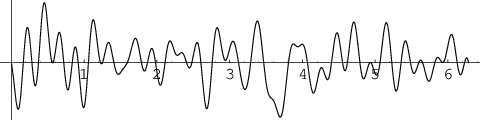
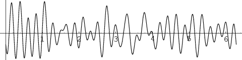
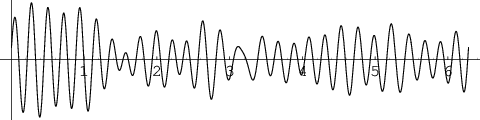
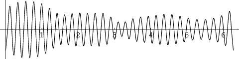
The Gauss model extends to entire functions of order , provided one incorporates a background field coming from the exponential factors of the Hadamard factorization of the function. For such functions there is a general phenomenon that differentiation smooths out irregularities in the distribution of zeros. See [6] for details. If the zeros are located in a strip around the real axis and their initial distribution is not too irregular, then repeated differentiation leads the zeros to approach equal spacing. This regular spacing is known as the crystalline configuration [2] and we view the process of repeated differentiation as a toy model of crystallization in one dimension. According to the Gauss model, regular spacing is the equilibrium position and differentiation moves the function toward equilibrium. See Figure 1 for an illustration.
We now describe the functions we study and then discuss our results.
A random trigonometric polynomial of degree is a function of the form
| (1.1) |
where and are random variables. In this paper we will assume that the and are independent real Gaussian distributed with mean and variance , and usually we further assume that the variances are all equal.
Our concern is with the properties of the real zeros of . Generally will not have all of its zeros real, but the high derivatives of will have mostly real zeros, and those zeros will be close to equally spaced. This can be seen in Figure 1. This is a general property [6] of real entire functions of order , but in the case of trigonometric polynomials this is easy to see. The th derivative of is
where for simplicity we have assumed is a multiple of , For large the terms dominate. So the zeros of are close to the zeros of for some real and , and those zeros are real and equally spaced.
Another general property of repeated differentiation of real entire functions of order is that the discrepancy from equal spacing of zeros of the th derivative scales as . See Theorem 2.4.2 of [6]. In the case of random trigonometric polynomials we are able to obtain more precise information. We describe this in the next section.
2. Statement of results
In this section is a random trigonometric polynomial of the form (1.1) for which the and are independent Gaussian distributed random variables with mean 0 and identical variance. We wish to measure the rate at which the real zeros of the th derivative approach equal spacing as . We consider the pair correlation function of the zeros of , defined as
| (2.1) |
where
| (2.2) |
Here is the Dirac -function at , and stands for expected value. Thus, is the density function of real zeros of , and is the density function of differences of real zeros.
Since measures the differences between zeros, if the zeros are almost regularly spaced then will be large when is close to a multiple of the average zero spacing and it will be small otherwise. In other words, we expect that should approach a sum of -functions at the integers as . Bogomolny, Bohigas, and Lebœuf [2] obtain a general expression for the pair correlation function of the real zeros of a random trigonometric polynomial. From their results (which we describe in Section 4) we obtain a formula for , which we plot for in Figure 2. Note that the case is from [2].
The plots in Figure 2 use the following normalization. We rescale the polynomial so that the average spacing between zeros is , that is, we are actually considering the function . As we describe in Section 3, as the function has the expected fraction
| (2.3) |
of real zeros. So is the average gap between consecutive real zeros, and that is the spacing between the peaks in the pair correlation functions in Figure 2. Note that is also the density of real zeros. So the pair correlation function will equal on average, which can also be seen in Figure 2.


We give an asymptotic formula for the pair correlation function as . As in the general case [6] we find a discrepancy from equal spacing, and furthermore we find that the nearest-neighbor spacing has (appropriately rescaled) distribution function
| (2.4) |
centered at . In particular, the discrepancy from equal spacing is not Gaussian. The precise statement is
Theorem 2.1.
As , the pair correlation function of the real zeros of approaches a sum of Dirac -functions at the nonzero integers. The -function near the positive integer is given by
| (2.5) |
as .
The proof is given in Section 4.1 Note that the total area under is , which shows that the above Theorem does in fact identify the -function near the integer .
Since the zeros of are close to equally spaced, the peak of near is almost completely due to nearest-neighbor spacings. Thus, we can read the nearest-neighbor distribution from the pair-correlation function, as given in (2.4). In fact, we can also read off the next-nearest neighbor spacing (and all of the other neighbor spacings), as , from the pair correlation function. Up to rescaling, all of those distributions are the same. This shows that there are long-term correlations between the zeros, otherwise, for example, the next-nearest neighbor distribution would be the convolution of the nearest neighbor distribution with itself.
One motivation for this work is to understand, in general, the effect of differentiation on the statistics of zeros for functions which have all their zeros on a line. In particular, we would like to understand the effect of differentiation on the repulsion between zeros. For example, if has only real zeros and the zeros have the same statistics as the eigenvalues of the classical random matrix -ensemble, then the zeros of have repulsion of order . For the derivative , it is reasonable to conjecture that the zeros would have repulsion of order , because pairs of close zeros of occur when has three closely spaced zeros. This topic is of interest to number theory [5]. Unfortunately, the calculations in this paper do not shed light on this phenomenon because the zeros of random trigonometric polynomials are not in general all on the real line. We find that all derivatives of a random trigonometric polynomial have linear repulsion between zeros, and show that this is due to the fact that each derivative moves new zeros onto the real line, and those new zeros show linear repulsion from each other. See Section 4.2.
3. Random trigonometric polynomials
We assume that is a random trigonometric polynomial of the form (1.1), where the and are independent real normally distributed random variables with mean 0 and identical variance .
The expected fraction, , of real zeros of is given in (2.3). This result is due to Dunnage [3]. It follows directly from the Kac-Rice formula, which we give in Lemma 3.1.
Note that the original polynomial has on average real zeros, the 4th derivative has more than 90% of its zeros real, and one must take 49 derivatives in order to expect 99% real zeros. Note that these are asymptotic results, and one can obtain exact formulas for any . For example, the , example at the bottom of Figure 1 expects to have 96.96% real zeros, and this is approximately 1.4% larger than the asymptotic estimate (2.3).
We now derive (2.3).
Lemma 3.1.
In the case of of the form (1.1) we have
If all the coefficients of have equal variance , then the th derivative can be viewed as a random trigonometric polynomial of the form (1.1) where the coefficients and have variance . So for the th derivative we have
| (3.1) |
and
| (3.2) |
as . From this, formula (2.3) for the fraction of real roots follows immediately.
4. Pair correlation of the real roots
We use a result of Bogomolny, Bohigas, and Lebœuf [2] to compute the pair correlation function of the real zeros of .
Lemma 4.1 (Appendix B of [2]).
Suppose
is a random trigonometric polynomial, where the and are independent real Gaussian distributed random variables with mean 0 and variance . The expected value of the pair correlation function of the real zeros of is given by
| (4.1) |
where
| (4.2) |
with
| (4.3) |
We apply the Lemma to with . So we have
| (4.4) |
as . To determine asymptotics for , and , we use the fact that for continuous functions
We change variables , so in the variable the mean spacing between zeros of is unity. We have
| (4.5) | ||||
| (4.6) | ||||
We let denote the pair correlation function of the real zeros of the th derivative , where is given by (1.1) with all and independent identical Gaussian, and we normalize by dividing by the square of the overall zero density . As we have
| (4.7) |
where
| (4.8) |
with
| (4.9) |
Plots of for are given in Figure 2.
4.1. Large asymptotics of the pair correlation
We determine the rate at which , appropriately rescaled, approaches a sum of -functions at the integers.
We first find asymptotic formulas for , , and . Using a geometric series expansion for and , and using integration by parts followed by a geometric series expansion for , , and , we find (with the help of a computer algebra package), that
| (4.10) | ||||
| (4.11) | ||||
| (4.12) | ||||
| (4.13) |
We see that and are generally of size , while is generally of size . But for we see that is of size . Thus, as , if then , otherwise . This is exactly what one should expect because is approaching a sum of -functions at the integers. We now express this more precisely.
The minima of are not exactly at the integers, but they are shifted over to approximately for . This is also what one would expect because the mean spacing of the real zeros of is approximately . We will verify this directly from the above formulas. Differentiating with respect to we have
| (4.15) |
We are thinking of as fixed and large, so the minimum of is close to the solution to
| (4.16) |
which is equivalent to
| (4.17) |
The solutions with near an integer correspond to the minima of , so writing and , we find
| (4.18) |
as expected.
To show the shape of the -functions, we expand near the minima of . For positive integers we find that
| (4.19) |
Also,
| (4.20) | ||||
| (4.21) |
Thus, , so we obtain Theorem 2.1.
4.2. Repulsion between zeros
In [2] it was found the the real zeros of have linear repulsion. We find that the real zeros of also show linear repulsion.
Computing the small asymptotics of (4.9) we find that
| (4.22) | ||||
| (4.23) |
as . So for every derivative we have linear repulsion between zeros. This appears to contradict the expectation that differentiation increases the repulsion between zeros. However, there is a simple explanation. Each derivative causes more zeros to fall onto the real line. These “new” zeros can be closely spaced, as illustrated in Figure 3.
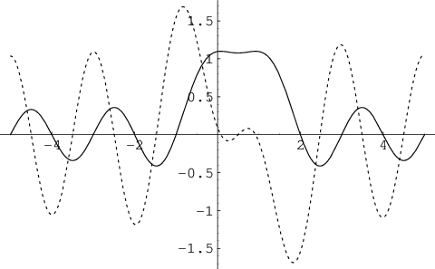
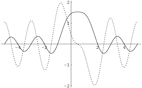
In Figure 3, all of the zeros are spaced one unit apart, except for two zeros which have been moved to have imaginary part and real part the midpoint of the resulting gap. In the left plot we have and in the right plot . Moving the complex zeros to have imaginary part
| (4.24) |
gives a triple zero of the derivative, so values slightly less than this give closely spaced zeros.
Since the fraction of new real zeros for the th derivative is
| (4.25) |
which is of the same magnitude as the linear repulsion, we see that the new zeros lead to repulsion of magnitude . It seems reasonable to believe that this accounts for all of the linear repulsion, but we have not been able to verify this.
References
- [1] A.T. Bharucha-Reid and M. Sambandham, Random Polynomials, Academic Press, 1986.
- [2] E. Bogomolny, O. Bohigas, and P. Lebœf, Quantum Chaotic Dynamics and Random Polynomials J. Statist. Phys. 85 (1996), no. 5-6, 639–679.
- [3] J.E.A. Dunnage, The number of real zeros of a random trigonometric polynomial, Proc. London Math. Soc., 16:53-84, 1966.
- [4] A. Edelman and E. Kostlan, How Many Zeros of a Random Polynomial are Real? Bull. Amer. Math. Soc. 32, 1-37, 1995.
- [5] D.W. Farmer and S. Gonek, The pair correlation of zeros of the derivative of the Riemann -function, in preparation.
- [6] D.W. Farmer and R.C. Rhoades, Differentiation Evens Out Zero Spacings, Trans. Amer. Math. Soc., 357 (2005), no.9, 3789–3811.
- [7] M. Kac, On the average number of real roots of a random algebraic equation, Bull. Am. Math. Soc 49, (1943), 314-320.
- [8] S.O. Rice, The distribution of maxima of a random curve, Amer. Jour. Math 61, (1939), 409-416.