General Covariance in
Algebraic Quantum Field Theory
Romeo Brunetti,a Martin Porrmanna and Giuseppe
Ruzzib
romeo.brunetti@desy.de, martin.porrmann@desy.de,
ruzzi@mat.uniroma2.it
a II. Institut für Theoretische Physik, Universität Hamburg Luruper Chaussee 149, 22761 Hamburg, Germany
b Dipartimento di Matematica, Università di Roma "Tor Vergata” Via della Ricerca Scientifica, 00133 Roma, Italy
Chapter 1 Introduction
1.1 The Problem of General Covariance
The question of general covariance of physical theories in space and time can be traced back to the famous debate between Gottfried Wilhelm Leibniz and Samuel Clarke (the latter assisted by Sir Isaac Newton) on the ontological status of space in the years 1715–1716 [1], the central question being if space exists as a substance or as an absolute being and absolute motion is present (Clarke) or if it is constituted only in relation to co-existent things allowing for relativism in motions only (Leibniz). This kind of problems also played an important role when the general theory of relativity was being developed in the years around 1910. While Albert Einstein first characterized generally covariant field equations as inadmissible since they did not determine the metric field uniquely as shown in the hole argument (Lochbetrachtung) in the appendix of [56], he later accepted [55] that all physical laws had to be expressed by equations that are valid in all coordinate systems, i. e., which are covariant (generally covariant) under arbitrary substitutions.11 1 “Die allgemeinen Naturgesetze sind durch Gleichungen auszudrücken, die für alle Koordinatensysteme gelten, d. h. die beliebigen Substitutionen gegenüber kovariant (allgemein kovariant) sind.” [55, p. 776] The hole argument was dismissed by the reasoning that it is not the spacetime metric that has to be fixed uniquely by the field equations, but only the physical phenomena that occur in spacetime need to be given a unique expression with reference to any description of spacetime. All physical statements are given in terms of spacetime coincidences; measurements result in statements on meetings of material points of the measuring rods with other material points or in coincidences between watch hands and points on the clockface. The introduction of a reference system merely serves the easy description of the totality of all these coincidences (point-coincidence argument) [55, p. 776f].22 2 “Da sich alle unsere physikalischen Erfahrungen letzten Endes auf solche Koinzidenzen zurückführen lassen, ist zunächst kein Grund vorhanden, gewisse Koordinatensysteme vor anderen zu bevorzugen, d. h. wir gelangen zu der Forderung der allgemeinen Kovarianz.” [55, p. 777]
In this paper we give an account of new results on how this concept of general covariance is approached within the framework of algebraic quantum field theory, a task already put forward in the Gibbs lecture on Missed Opportunities held by Freeman Dyson in 1972 [54] (including a warning on the necessity of a “delicate weaving together of concepts from differential geometry, functional analysis, and abstract algebra”). A couple of articles on this problem have been published since then [60, 8, 9]. But the introduction of notions from category theory into these attempts sheds new light on the problem at hand, opening up a new and promising perspective [23]. We will turn to a presentation of these ideas after a short account of the ideas of algebraic quantum field theory in this Introduction.
1.2 Algebraic Quantum Field Theory
The use of algebraic concepts has been one of the great achievements in the development of a theory for the description of microscopical phenomena in the middle of the 1920’s, when a consistent description as quantum mechanics was presented by Max Born, Pascual Jordan, Werner Heisenberg and Paul Adrien Maurice Dirac [73, 18, 42, 17]. For quantum mechanics an algebraic generalization of the formalism has been presented in [78]. With respect to physical systems of infinitely many degrees of freedom (quantum field theory), a mathematically sound foundation for an algebraic approach has been given by Irving Segal in the 1940’s [107], which later, following the introduction of the concept of weak equivalence of representations of the algebras by James Michael Gardner Fell [57], was supplemented by the principle of locality for physical reasons in the work of Rudolf Haag [66] and Rudolf Haag, Hans-Jürgen Borchers and Bert Schroer [16] and axiomatized in the innovative publication An Algebraic Approach to Quantum Field Theory by Rudolf Haag and Daniel Kastler [70] in 1964.
In the following years the mathematical framework thus acquired proved to be a suitable basis for the formulation and investigation of structural questions of quantum field theory. Among these are counted the understanding of the multiparticle structure of field theory in the Haag-Ruelle scattering theory [67, 100], the structure of inner symmetries in the Doplicher-Haag-Roberts (DHR) theory [45, 46, 47, 48] and in the Doplicher-Roberts (DR) duality theory [50, 51]. Since the general assumptions of the algebraic approach were not restrictive enough to exclude quantum field theoretic models exhibiting unphysical behaviour, attempts were made to supplement the structure by specific information about the phase-space structure of quantum field theory. These fall into two different groups: First, there are qualitative requirements in terms of compactness conditions [71, 61]; second, quantitative requirements using the mathematical notion of nuclearity were introduced [36, 34]. The former ones proved to be successful in eliminating quantum field theoretic models without a particle interpretation, while the second group was devised with thermodynamical applications in mind (cf. also [31, 30, 32]). They are an essential ingredient also in the analysis of scattering states in theories with long-range interactions via the concept of particle weights [35] in the attempt to generalize an ansatz by Araki and Haag [7] for the description of scattering states in terms of local observables (cf. [93, 94] for a thorough exposition).
The investigation of thermodynamic equilibrium states within the framework of algebraic quantum field theory is based on the algebraic reformulation of the Gibbs ansatz for statistical mechanics [69] based on the so-called Kubo-Martin-Schwinger (KMS) condition [87, 90]. Whereas the Gibbs ansatz requires the spectrum of the Hamiltonian to be discrete (system in a box), the KMS condition is mathematically well-defined without this restriction, giving direct access to the thermodynamic limit. Considerable efforts have been undertaken since then to further generalize this condition to relativistic systems [19] and also to develop a mathematically sound description of states not in equilibrium [33]. Closely connected with these questions is the Tomita-Takesaki modular theory, a cornerstone in the development of the theory of operator algebras and important also in applications to physical problems (cf. [14, 15] for an overview).
A comprehensive exposition of the principles and achievements of the algebraic approach can be found in the monograph by Rudolf Haag [68]. To the open problems of algebraic quantum field theory belongs the task to exhibit physically relevant interacting models that meet the axioms (this is taken up in the approach of constructive quantum field theory). Furthermore, the incorporation of gravity into this framework is a major desideratum with all the pertaining questions: description of equilibrium and nonequilibrium states in curved spacetimes, their implications on cosmological questions, and a host of other exciting problems.
1.3 Observables, States and Experiments
Information on physical systems is gathered by performing experiments, i. e., one prepares the physical system in a clear-cut way to have it in a certain state (or, more generally, in a mixture of states as a result of an incomplete preparation) which is the embodiment of all information that can possibly be gained, and then one has it interact with a measuring apparatus, the observable , which upon interaction reveals a certain change of its (macroscopic) properties. The measurement results are conveniently represented by real numbers so that formally we have to deal with a mapping
| (1.1) |
as the basis of any theoretical attempts to the description of nature. A thorough analysis of this scheme has been given by Huzihiro Araki in his lectures at the ETH Zurich [5, 6] and constitutes the basis for the corresponding discussion in [4]. Due to the fact that different procedures might result in the preparation of the same state of the physical system and that different measuring devices might return the same information about this state at hand, these notions refer to equivalence classes of preparation and measurement procedures rather than to individual ones.
Moreover, the science of physics is concerned with phenomena that can be reproduced (the theory of a single event being a futile venture) so that measurements are always concerned with ensembles representing a physical system in the same state. Apart from the limited accuracy of any actual measurement, this fact forces one to look for a probabilistic description of experiments; not the individual measurement result is decisive, but rather the probability distribution as the outcome of many (in principle, indefinitely many) experiments is the fact to be explained by a consistent theory. While in classical physics this indeterminacy of the results is ascribed solely to the limited accuracy in the preparation and measurement procedures, the developed theory giving definite predictions on the outcome of future experiments, this situation is changed drastically in quantum physics, where in principle only statistical assertions are possible.
States of a physical system either being the result of a complete preparation as pure ones or else the upshot of an incomplete preparation as a mixture, i. e., a convex combination of the former pure states, the mathematical structure of the state space as a convex set is evident. The general formulation (1.1) takes the shape of a dual pairing,
| (1.2) |
where the structure of the set of (equivalence classes of) observables is not fixed like that of . One proposal for its structure is that of a Jordan algebra [78] with the product defined by
| (1.3) |
Note that the first expression of only involves scalar multiples, sums and powers of elements of , not the product of and like the second one. A comprehensive presentation of Jordan algebras and their state spaces can be found in [3, Part I] (see also [88]). A theory for propositions about quantum systems has been developed under the term quantum logic. Garrett Birkhoff and John von Neumann revealed their structure of an orthocomplemented lattice [12]. If this is supplemented by the assumptions of semi- or orthomodularity, one can establish that the propositions are isomorphic to the set of orthogonal projection operators on a Hilbert space. A comprehensive presentation of orthocomplemented modular lattices is to be found in [109]. In view of these investigations it is not a far-fetched assumption to consider the structure of (1.2) as that of a dual pair of a ∗-algebra with a state space as the normalized part of its (algebraic or topological) dual. Normalization is required here in order for a probabilistic interpretation to be possible.
1.4 -Algebras, States and Representations
Quantum mechanics can conveniently be formulated with reference to a certain Hilbert space, the unit rays of which represent the states of the physical system under consideration while the self-adjoint operators stand for the measurements. In this way the set of measurements acquires the structure of the self-adjoint part of a concrete ∗-algebra of operators on a Hilbert space. Segal [107] had pointed to the fact that questions of physical interest could be answered without having to select a certain Hilbert space, if the measurements were part of a -algebra , i. e., a Banach∗-algebra with the additional property
| (1.4) |
This idea was absorbed by Haag and Kastler in 1964 [70] who proposed not to consider just one single -algebra but rather a net of -algebras associated with bounded regions of spacetime,
| (1.5) |
claiming that the physical content of a theory is encoded in this mapping. Thereby they stressed the local nature of measurements in much the same spirit as Einstein did in 1916 [55] by stating [70, p. 851] that “ultimately all physical processes are analyzed in terms of geometric relations of (unresolved) phenomena.”
The net (1.5) of local -algebras is supposed to be subject to the following conditions (the existence of the quasi-local algebra is in fact not an assumption, but a consequence of the assumed isotony):
-
Isotony: For any two bounded regions and
(1.6a) -
Locality: If the bounded regions and are spacelike separated, i. e., belongs to the spacelike complement of , formally , then
(1.6b) Note that at this point the net structure of enters, i. e. the directedness of the index set, implying that any two local algebras are contained in a larger one pertaining to a region that comprises both and .
-
Quasi-Local Algebra: The set-theoretic union of all local algebras generates a normed ∗-algebra which upon completion is again a -algebra called the quasi-local algebra.33 3 This minimal -algebra is well-defined on account of isotony and called the inductive limit of the family .
-
Special Relativistic Covariance: If there is a representation of the proper orthochronous Poincaré group on the quasi-local algebra by automorphisms, , then these automorphisms should act covariantly, i. e.
(1.6c) where denotes the image of under the Poincaré transformation.
The actual measurements are represented by the self-adjoint elements of the corresponding -algebras, while the states are the positive, normalized, linear functionals on the quasi-local algebra .
-
Positivity: For any element
(1.7a) -
Normalization: The norm of as an element of the topological dual of is ,
(1.7b)
In view of the probabilistic interpretation, the real number that the state returns when applied to a self-adjoint element of is considered as the expectation value (mean value) resulting from measuring the corresponding observable in the ensemble represented by .
The algebra is not considered as a concrete algebra, i. e., an algebra of bounded linear operators on a given Hilbert space. Instead it can be represented as such in various ways on different Hilbert spaces, where the term representation refers to a ∗-homomorphism (denoted ) that associates bounded operators on a certain representation Hilbert space with elements , respecting the algebraic structure of as well as its ∗-operation. In general there will exist an abundance of different representations of that are not unitarily equivalent, i. e. connected by a unitary operator , while some of them might be physically equivalent in the weak sense of Fell [57] (cf. [70, p. 851]). In fact, via the GNS (Gel’fand, Naimark, Segal) construction, every state on is associated with its own representation . In the years to come this general framework, supplemented by physically motivated further requirements depending on the investigations to be performed, has proven to constitute a flexible foundation to tackle structural questions of quantum field theory. Among the most important contributions rank investigations on nuclearity and the split property [28, 49], equilibrium and nonequilibrium physics [19, 33], modular theory [15], conformal field theory models [83], energy inequalities [58] and the approach to noncommutative spacetime [44]. Apart from that, a sound formulation of perturbation theory has been given within the algebraic approach to quantum field theory [21, 22]. This review will concentrate on the investigation of general covariance as one of the many examples referred to above for research in this domain.
Chapter 2 Locally Covariant Quantum Field Theory
2.1 Preliminaries
The following exposition will be concerned with four-dimensional, globally hyperbolic spacetimes. Therefore, also to fix our notation, we will summarize some of their basic properties; for a thorough discussion the reader is referred to [72, 111]. The condition of global hyperbolicity does not seem to be very restrictive on physical grounds, its main purpose being to rule out certain causal pathologies.
A spacetime is denoted by the pair , where is a smooth (i. e. , Hausdorff, paracompact and connected) four-dimensional manifold and is a Lorentzian metric on it with signature . Not to overburden the formalism, we will usually only write for the manifold, implicitly including its metric . This also applies to other manifolds of the said type, where the metric shares the diacritical signs (primes, subscripts, …) differentiating the manifolds. The spacetimes are moreover assumed to be oriented and time-oriented. Time orientability requires the existence of a vector field on which is timelike everywhere, i. e., at all points of . Nonspacelike tangent vectors are called future directed or past directed if, in relation to the vector field , one has or , respectively. This defines a time direction on which is globally consistent. A smooth curve , a connected subset of , with tangent vector is called future directed timelike if and for all points of ; it is called future directed causal if and on all of . is said to be past directed timelike or past directed causal if in the above definitions the Lorentz product of and is negative. If the nonspacelike curve is future directed and the point exists in it is called the future endpoint. The definition of a past endpoint requires to be past directed and replaced by . A curve is called future inextendible (past inextendible) if the corresponding endpoints do not exist; it is called inextendible if it is future and past inextendible [91]. Given a point , the set consists of all points in that can be connected to by a future directed timelike curve, while consists of all points in that are connectable to by some future directed causal curve with . Replacing the requirement of future-directedness by past-directedness, one gets the sets and , respectively.
Two subsets and in are called causally separated if it is impossible to connect them by a causal curve, i. e., if for all , has empty intersection with (the bar denotes closure with respect to the induced topology of the manifold ). The largest open set in that is causally separated from is called the causal complement of denoted . A subset of is called achronal if it does not contain any pair of points , with . For a closed achronal set the future domain of dependence is the set of all points with the property that any past inextendible causal curve through intersects ; the past domain of dependence is defined using future inextendible curves through intersecting . The full domain of dependence is the union of and .
An oriented and time-oriented spacetime is called globally hyperbolic if for each pair of points , the intersection of and is compact. This property has been shown to be equivalent to the existence of a smooth foliation of in terms of Cauchy surfaces by Bernal and Sánchez [11]. A Cauchy surface is a smooth hypersurface of that any inextendible causal curve intersects exactly once. In globally hyperbolic spacetimes the global Cauchy problem (inital value problem) for linear hyperbolic wave equations is well-posed, and these wave equations possess unique retarded and advanced fundamental solutions. While the property of global hyperbolicity does not refer to any spacetime isometries, the concept of isometric embeddings will be important later. Let and be two globally hyperbolic spacetimes, then we call a mapping an isometric embedding of into if is a diffeomorphism onto its range , i. e., the map is a diffeomorphism, and if is an isometry, i. e., .
Given a globally hyperbolic spacetime , we want to introduce families of open subsets which will be used as an index set for nets of local algebras according to (1.5) and prove their stability under isometric embeddings.
Globally hyperbolic regions
Let be the collection of subsets satisfying the following properties:
- (i)
is an open, arcwise-connected, relatively compact set, and .
- (ii)
If , , then is either empty or contained in .
It turns out by this definition that is a basis for the topology of and that any element of with metric and induced orientation and time orientation is again a globally hyperbolic spacetime. There a some straightforward geometrical results for .
Lemma 2.1.
Let be a globally hyperbolic spacetime, then the following assertions hold:
- (i)
Let , be such that . Then there exists such that .
- (ii)
For any there are , such that and .
- (iii)
Let and let be an open set with , then .
This lemma can be used to show that the only obstruction to the directedness of the family , viz. the fact that for any pair , there is such that , is the compactness of Cauchy surfaces.
Lemma 2.2.
Let the globally hyperbolic spacetime possess noncompact Cauchy surfaces, then is directed.
Lemma 2.3.
Consider globally hyperbolic spacetimes and with an isometric embedding and define
Then
Proof.
We stress that the collection possesses elements which are not simply connected subsets of and elements whose causal complement is not arcwise-connected. Problems associated with this topological feature can be avoided by passing to certain subcollections like diamond regions.
Diamond regions
The set of diamonds of [102] consists of open subsets of , called diamonds, for which there exist a spacelike Cauchy surface , a chart of and an open ball of such that
is said to be based on , i. e., is the base of . Any diamond is an open, relatively compact, arcwise- and simply connected subset of , and its causal complement is likewise arcwise-connected. Furthermore, given a diamond , there exists a pair of diamonds , with
| (2.1) |
The set of diamonds is a basis for the topology of .
Lemma 2.4.
Consider globally hyperbolic spacetimes and with an isometric embedding and define
then
Proof.
We prove the inclusion . Let be a diamond of , i. e., there exist a spacelike Cauchy surface of , a chart such that , where is a ball of such that . Let be a ball of with and . Note that is a compact, spacelike acausal open set of with boundaries and with a nonempty complement. By [10], there exists in a spacelike Cauchy surface such that . Define and . The pair is a chart of and . Finally, observe that, due to the properties of , we have , viz. . The proof of the reverse inclusion is very similar. ∎
There are other interesting collections of subsets of , e. g. the family of regular diamonds used in [65] that contains the family of diamonds introduced above as a subset and has the same stability property.
2.2 Quantum Field Theories as Covariant Functors
The investigations to be presented draw upon the theory of categories and functors. The reader not familiar with these concepts can find an introduction to the field in [89]. The two categories to be used in this chapter are
-
This category has as objects the collection consisting of all four-dimensional, globally hyperbolic spacetimes which are oriented and time-oriented. The morphisms between two such objects and constitute the collection and are those isometric embeddings which satisfy the following additional constraints:
- (i)
if is any causal curve and , then the whole curve must be contained in the image , i. e., for all ;
- (ii)
the isometric embedding preserves orientation and time-orientation of the embedded spacetime.
The composition for any morphisms and in and , respectively, is the set-theoretic composition of maps . is thus a well-defined map which obviously is a diffeomorphism onto its range and is evidently isometric. Likewise, the properties (i) and (ii) are obviously fulfilled so that indeed . The associativity of the composition rule is an immediate consequence of that of the set-theoretic composition of maps. The requirement for categories that each has to possess a unit element is fulfilled by the identity map , .
- (i)
-
This category has as objects the class formed by all unital -algebras, while the collection of morphisms between the objects (algebras) and are the faithful (injective) unit-preserving ∗-homomorphisms. Given such morphisms and belonging to and , respectively, their composition is again the composition of maps and easily seen to be an element of . The unit element of for any algebra is the identity , .
Remark 2.5.
- (A)
The first requirement (i) that the morphisms of have to satisfy enforces the induced and intrinsic causal structures to coincide for the embedded spacetime (cf. [84]). The second condition (ii) could be relaxed so that the possible reversal of orientation in space and time allows for a a discussion of PCT theorems.
- (B)
The framework presented above is open to variations depending on the problems to be investigated. The algebras that constitute the objects of could be replaced by general ∗-algebras, Borchers algebras or von Neumann algebras. With respect to , the spacetimes could have less specific properties or even be endowed with additional features like spin structures as in [41, 110].
Now we introduce the concept of a locally covariant quantum field theory which encodes the generally covariant principle of locality.
Definition 2.6.
- (a)
A locally covariant quantum field theory is a covariant functor between the two categories and , i. e., writing for the image of the morphism under the functor , the following mappings
have to satisfy the covariance properties
(2.2a) (2.2b) for all morphisms , and all spacetimes .
- (b)
A locally covariant quantum field theory given by the covariant functor is called causal if for morphisms , , , embedding and in the common spacetime such that the sets and are causally separated in , the corresponding algebras in commute, i. e.,
(2.3) where denotes the commutator of any pair and of -subalgebras contained in a common larger one.
- (c)
A locally covariant quantum field theory given by the covariant functor obeys the time slice axiom if for any with the property that contains a Cauchy surface for we have
(2.4)
A locally covariant quantum field theory given by the functor assigns to any globally hyperbolic spacetime a corresponding -algebra in such a way that the algebras can be identified when the spacetimes are isometric. This is the mathematically precise way to express the requirement for a unique expression for physical phenomena in spacetime regardless of the selected coordinate system as explained on p. 1. The term local is used here in the sense of geometrically local which is not to be confused with locality in the sense of Einstein causality. Causal properties are specified only in (b) and (c) of Definition 2.6. Here, causality means that elements of the algebras and , respectively, commute in the larger algebra when the subregions and of are causally separated with respect to the metric on . This property is expected to hold generally for observable quantities which can be localized in certain subregions of spacetimes. The time slice axiom (c) (also called strong Einstein causality, or existence of a causal dynamical law, cf. [110]) states that the algebra of observables on a globally hyperbolic spacetime is already determined by the algebra of observables localized in a neighbourhood of any Cauchy surface.
2.3 Recovering Algebraic Quantum Field Theory
In this section we will demonstrate that and how the setting of algebraic quantum field theory on a fixed globally hyperbolic spacetime as described in Section 1.4 can be regained from a locally covariant quantum field theory given by a covariant functor with the properties listed in the preceding Section 2.2. The general assumptions on the net of local algebras (1.5), i. e. isotony (1.6a) and locality (1.6b), are supplemented here by the requirement that all the local algebras as well as the quasi-local algebra contain a common unit .
Let be an object in . Given , denotes the Lorentzian metric restricted to so that (with the induced orientation and time orientation) is a member of . The corresponding injection , i. e. the identity map restricted to , is an element in . Using this notation we can formulate the following assertion.
Proposition 2.7.
Let be a covariant functor with the properties stated in Definition 2.6. Define a map via
where is an abbreviation for . Then the following statements hold:
- (i)
The map fulfills isotony, i. e., for all ,
- (ii)
Assume that there exists a group of isometric diffeomorphisms (i. e. ) preserving orientation and time orientation. Then there also exists a representation of the group by -algebra automorphisms of the -algebra generated by the net such that
(2.5) - (iii)
If in addition the functor is causal, then for all subsets , that are causally separated from each other the corresponding algebras commute,
Proof.
- (i)
The proof of the first statement uses the covariance properties of the functor . To demonstrate isotony, let and be elements of with . Let be the canonical embedding obtained by restricting the identity map on to , then . With , etc., covariance of the functor implies , and therefore
since by the very properties of the functor .
- (ii)
To prove the second statement, let be a diffeomorphism preserving the metric as well as time orientation and orientation. The functor assigns an automorphism to this special diffeomorphism. To the map with the functor associates a morphism . Hence
Since , the definition of as the restriction of to yields an automorphism with the required properties. The feature of a group representation is an immediate consequence of the covariance properties of the functor which imply for any pair of elements , together with (2.5). Therefore, one concludes that indeed .
- (iii)
If and are causally separated elements of , one can find a Cauchy surface in and a pair of disjoint subsets and of , both connected and relatively compact, which satisfy , , . The sets are causally separated members of , and, when equipped with the appropriate restrictions of the metric , they are globally hyperbolic spacetimes in their own right, naturally embedded into . According to the causality assumption on , the algebras are pairwise commuting subalgebras of and, due to isotony, which implies that also . This completes the proof. ∎
2.4 Quantum Fields as Natural Transformations
In the previous section a quantum field theory has been defined in terms of a covariant functor: an algebra is mapped into another algebra via the endomorphism , but a priori nothing is said about how specific elements of the algebras are mapped onto each other by that transformation. In this section the possibility to define locally covariant fields is considered, their importance lying in the potential construction of fields that only locally depend on the geometry. The physical meaning underlying this construction is the idea that such fields might serve as carriers of information from one point of a spacetime to another in absence of global isometries like translations, or even from one spacetime to another one. The definition of locally covariant quantum fields to be given below generalizes the approach of Gårding and Wightman, who characterized quantum fields as operator-valued distributions. Here the distributions are not specified explicitly in this way, but can take values in a topological ∗-algebra instead.
We consider a family of topological ∗-algebras that are indexed by all spacetimes in . For each spacetime a quantum field is defined as a generalized algebra-valued distribution, i. e. a map which is supposed to be continuous, but not necessarily linear. The collection of all these mappings constitutes the family . In addition, we demand that for any there exists a continuous endomorphism so that
where is any test function and . The family with these covariance conditions is called a locally covariant quantum field. This simple description has a functorial translation to be outlined next.
Again we consider the category and furthermore introduce the category consisting of topological ∗-algebras with unit elements as objects and of continuous ∗-endomorphisms as morphisms. This means that is an element of if it is a continuous, unit-preserving, injective ∗-morphism. Let denote the category containing all possible test function spaces over as objects, i. e., the objects are all spaces of smooth, compactly supported test functions on for all , and the morphisms are all possible push-forwards of isometric embeddings . The action of any push-forward on an element of a test function space has been defined in the preceding paragraph, and it clearly satisfies the requirements for morphisms between test function spaces.
Now, let the locally covariant quantum field theory be defined as a functor according to Definition 2.6 with the modification that the category replaces the category ; again stands for whenever is any morphism in . Moreover, let be the covariant functor between and assigning to each the test function space and to each morphism of its push-forward: . as well as are regarded as subcategories of the category of all topological spaces, , leading to the following definition.
Definition 2.8.
A locally covariant quantum field is a natural transformation between the functors and , i. e., for any object there exists a morphism in such that for each morphism the following diagram commutes:
Explicitly,
which is the requirement of covariance for fields.
Remark 2.9.
- (A)
This definition is open to extensions. The test function spaces could be replaced by smooth, compactly supported sections of vector bundles, and as endomorphisms of these test section spaces one takes suitable pull-backs of vector-bundle endomorphisms. One can also include conditions on the wave front set of the field operators (cf. Definition 3.2 below).
- (B)
The notion of causality is introduced in an obvious way: A locally covariant quantum field is causal if and commute for all , such that .
- (C)
- (D)
We give some examples in Chapter 3.
2.5 On the Notion of State Space
We have seen previously that part of the physical description of a theory proceeds through the selection (preparation) of a suitable class of states. Here we attempt at a definition of a state space suitable for the description of a generally covariant quantum field theory.
Indeed, suppose that our theory is given in terms of a covariant functor . The question arises what the concept of a state might be in this case. The first, quite natural idea is to say that a state is a family indexed by the members in the object class , where each is a state on the -algebra . One might wonder if there are families of states that are distinguished by a property which in our framework would correspond to local diffeomorphism invariance, viz.,
for all . However, there is a simple argument that shows that the above property will, in general, not be physically realistic. We refer to [23] for a thorough explanation.
A crucial question is whether there exists a more general concept of invariance that can be attributed to families of states for a locally covariant quantum field theory given by a functor . We will argue that there is a positive answer to this question. To arrive at an explanation, let us fix some concepts that will turn out to be useful also in the subsequent chapters.
Folium of a representation
Let be a -algebra and be a ∗-representation of by bounded linear operators on a Hilbert space . The folium of , denoted , is the set of all states on which can be written as
where denotes the trace in . In other words, the folium of a representation consists of all density matrix states in that representation.
Local quasi-equivalence and local normality
Let be a locally covariant quantum field theory and let, for fixed , and be two states on . We call these states (or their GNS representations, denoted and , respectively) locally quasi-equivalent if for all the relation
| (2.6) |
is valid, where and is the natural embedding.
Moreover, we say that is locally normal to (or to the corresponding GNS representation ) if
| (2.7) |
for all .
It is known that quasifree states of the free scalar field on globally hyperbolic spacetimes which fulfill the microlocal spectrum condition (cf. Section 3.1) are locally quasi-equivalent. We also note that the property of a state to fulfill the microlocal spectrum condition is a locally covariant property (owing to the covariant behaviour of wavefront sets of distributions under diffeomorphisms [77]). Thus, for a locally covariant quantum field theory it is natural to assume that, if fulfills (any suitable variant of) the microlocal spectrum condition, then so does for any . In the case where also the folia of states (i. e. the folia of their GNS representations) satisfying the microlocal spectrum condition coincide locally, one thus obtains the invariance of local folia under local diffeomorphisms, more precisely, at the level of the GNS representations of and , one has
for all and all . All these properties are known to hold for quasifree states of the free scalar field fulfilling the microlocal spectrum condition on globally hyperbolic spacetimes.
Thus one sees that local diffeomorphism invariance really occurs at the level of local folia of states for . In this light it appears natural to give a functorial description of the space of states taking this form of local diffeomorphism invariance into account. To this end, it is convenient to first introduce a new category, the category of the set of states.
-
An object is a set of states on a -algebra . Morphisms between members and of are positive maps . In the present work, always arises as the dual map of a faithful -algebra endomorphism via
The category is therefore dual to the category . The composition rules for morphisms are thus obvious.
Now we can define a state space for a locally covariant quantum field theory in a functorial manner.
Definition 2.10.
Let be a locally covariant quantum field theory.
- (a)
A state space for is a contravariant functor between and :
where is a set of states on and is the dual map of ; the contravariance property is
together with the requirement that unit morphisms are mapped to unit morphisms.
- (b)
We say that a state space is locally quasi-equivalent if (2.6) holds for any pair of states , (with GNS representations , , respectively) whenever and .
- (c)
A state space is called locally normal if there exists a locally quasi-equivalent state space so that for each there is some (with GNS representation ) so that (2.7) holds for all and .
Some straightforward consequences of these definitions can be found in [23]. Further properties are outlined in the last chapter.
Chapter 3 Examples
3.1 Microlocal Analysis
This section serves the purpose of giving a self-contained introduction to definitions and results of Hörmander’s microlocal analysis that will be needed in the sequel. After having defined the wave front set of a distribution, we recall Hörmander’s results on the multiplication of distributions which extends to the composition of distribution-valued operators. Further details of this mathematical theory can be found in Hörmander’s monograph [77] and in the original sources.
The theory of wave front sets was developed in the 1970’s by Hörmander and Duistermaat [76, 52], following the work of Sato [105, 106]. Mathematicians use wave front sets () mainly as a tool in partial differential equations. These sets are refinements of the notion of the singular support of a distribution. One advantage of the use of wave front sets over singular supports is their providing a simple characterization for the existence of products of distributions, eliminating the difference between local and global results. Duistermaat and Hörmander [52] recognized a link between microlocal analysis and quantum field theory, but these results were rarely used in the physics literature.
In microlocal analysis the study of singularities is shifted from the base space to the cotangent bundle by localizing the distribution around the singularity followed by an analysis of the result in Fourier space. Let be a distribution and let be a smooth function with support in . By a well-known argument from the theory of distributions, the Fourier transform of yields a smooth function in frequency space with the following relation,
where denotes dual pairing. This result implies
Lemma 3.1.
Let and let be an open subset of . Then if and only if for each and each integer there is a constant such that
The singular support, , of is the complement of the largest open subset of where is smooth. Motivated by the previous lemma, the notion of wave front sets is a refinement of that of the singular support, taking into account the direction in which the Fourier transform does not strongly decay.
Definition 3.2.
The wave front set, , of is the complement in of the set of points in such that for some neighbourhood of and some conic neighbourhood of we have for each and each integer a constant such that
Note that a conic set has the property that with also the pair belongs to for all . The following remarks can easily be proved using Lemma 3.1.
Remark 3.3.
- (A)
Let be an open subset of , then for with wave front set the projection of this wave front set to the base point gives the singular support of .
- (B)
is a closed subset of since, by definition, each point has an open neighbourhood in consisting of such points, too.
- (C)
For all smooth test functions with compact support one has .
- (D)
For any distribution with wave front set the wave front sets of its partial derivatives are contained in .
Example 3.4.
- (1)
Let be a smooth function, then its wave front set is empty: .
- (2)
Consider the Dirac -distribution on . Its wave front set is .
It is worth recalling that the set of normal coordinates of the cotangent bundle over the base coordinates in allows for the identification of with and to consider as a subset of the cotangent bundle. Since the definition of wave front sets is local, it can be lifted to manifolds. An intrinsic definition of wave front sets will be given below.
In this chapter the manifolds considered are assumed to be -dimensional carrying a smooth Riemannian or semi-Riemannian metric.
Definition 3.5.
Let be an -dimensional smooth manifold with cotangent bundle and let , the distributions on . The point is called a regular directed point if and only if for all , for all and for any function with there exists a neighbourhood of in and a neighbourhood of in such that, for all and all , one has, uniformly in ,
Now, the wave front set, , of is the complement in of the set of all regular directed points of .
A useful application of wave front sets is the definition of products of distributions. Wave front sets provide a simple characterization for the existence of such products, which turns out to be sequentially continuous provided the wave front sets of the corresponding distributions are contained in a suitable cone in .
Definition 3.6.
Let be a closed cone in and let denote the subspace of distributions with wave front set contained in . A sequence of distributions in converges to a distribution if and only if the following conditions hold:
- (a)
converges to in (weakly);
- (b)
for all , there exist a test function with , a conic neighbourhood of in and a function as in Definition 3.5 such that for all
Note that every subspace contains all smooth test functions with compact support. Moreover, for there exists a sequence of compactly supported smooth functions such that in . Thus it is possible to choose their supports in an arbitrary neighbourhood of the support of .
Theorem 3.7.
Let be a smooth manifold and let , be two closed cones such that . Then the multiplication operator
extends to a unique sequentially continuous operator from the set to , where . In particular, the wave front sets are related by
| (3.1) |
Remark 3.8.
Note that for the product of two distributions and to exist it is sufficient that does not contain terms of the form .
3.2 The Scalar Klein-Gordon Field on a Fixed Spacetime Background
We describe quantum fields propagating on a four-dimensional Lorentzian manifold in terms of the general theory of quantized fields (cf. [59, 68, 112]). The manifold is assumed to be globally hyperbolic, i. e., it admits spacelike Cauchy hypersurfaces. We deal with the Gårding-Wightman approach to quantum fields [113] and its algebraic formulation by Borchers and Uhlmann [13, 108]. To each differentiable manifold is assigned a topological ∗-algebra constructed as follows: Elements in are sequences , , where and for . Addition and scalar multiplication are defined in the usual way for sequences with values in vector spaces, and the product in is determined as the sequence with
The ∗-operation is , where the elements of the sequence on the right-hand side are with the bar denoting complex conjugation. The unit element is . This algebra can be equipped with a fairly natural locally convex topology with respect to which it is complete. See [13, 108] for a further discussion of the Borchers-Uhlmann algebra (and also [60, 104] for the context of curved spacetime manifolds). A state , defined as a positive linear functional over , consists of a hierarchy of -point distributions, . Via the following GNS Reconstruction Theorem, every state satisfying local commutativity determines a Hilbert space, a vacuum vector in it and a representation of the algebra , thus linking the algebraic approach to the Hilbert space setting of Gårding and Wightman.
Theorem 3.9 (GNS Reconstruction).
For every state on the Borchers-Uhlmann algebra there is a GNS quadruple , unique up to unitary equivalence, such that for each and any test functions one has
Recall that a GNS quadruple satisfies the following properties, usually referred to as the (curved spacetime) Gårding-Wightman axioms:
- (A)
is a separable Hilbert space, is a dense subspace of , and the GNS vacuum is a distinguished vector in .
- (B)
The fields are operator-valued distributions, i. e., for all , the linear mapping
belongs to .
- (C)
The vacuum belongs to the subspace , and this space is an invariant domain for the fields, i. e., for each the domain of contains and .
- (D)
The fields are Hermitian, i. e., for each the domain of the adjoint of , denoted , contains and .
- (E)
The subspace is generated by applying finitely many smeared field operators to .
In flat Minkowski spacetime these axioms are supplemented by requiring covariance with respect to the Poincaré (inhomogeneous Lorentz) group and a condition on the spectrum stating that the Fourier transform of the -point function is concentrated at for , , …, .
The simplest and best studied example of a quantum field theory in curved spacetime is the scalar Klein-Gordon field. As shown by Dimock [40], its local -algebras can easily be constructed on each globally hyperbolic spacetime. As mentioned before, global hyperbolicity of the spacetime entails well-posedness of the global Cauchy problem for the scalar Klein-Gordon equation,
| (3.2) |
(for smooth, real-valued ), where is the covariant derivative of , and are constants, and is the scalar curvature of . Moreover, there exist uniquely determined advanced and retarded fundamental solutions of the Klein-Gordon equation, . Their difference is called the causal propagator of the Klein-Gordon equation. Let its range be denoted . It can be shown [40] that the definition
with the metric-induced volume form on , endowes with a symplectic form, so that is a symplectic space.
If the field arising from Theorem 3.9 satisfies the Klein-Gordon equation and its commutator is given by
we call a state of the Klein-Gordon field over . Not all states are believed to be physically meaningful. A condition expected to be satisfied by physically reasonable states is the Hadamard condition [39] which has been studied by various authors (cf. the references in Fulling’s book [63]). A mathematically precise definition of the Hadamard condition in terms of boundary values of certain complex-valued functions has been given by Kay and Wald in [85]. Radzikowski discovered [95] that an equivalent characterization of Hadamard states is possible in terms of their wave front sets. Using his results, Junker [79, 80] (note also the erratum to [80] in [81]) constructed Hadamard states for free scalar fields on arbitrary globally hyperbolic spacetimes. Radzikowski’s result can be recast in the following definition.
Definition 3.10.
Let be a quasifree state of the Klein-Gordon field over a globally hyperbolic manifold . Then is a Hadamard state if and only if its -point distribution has the wave front set
| (3.3) |
where means that there exists a lightlike geodesic connecting and with cotangent vectors at and at .
A state is called quasifree if and only if all its odd -point distributions vanish and the even ones satisfy
| (3.4) |
where denotes a partition of the set into subsets which are pairings of points, labelled by . The ordering of points in is preserved, e. g., , and two arguments never coincide so that the product exists whenever are distributions.
Using Theorem 3.7 in connection with (3.4), the wave front set of is seen to satisfy
| (3.5) |
where denotes a nonempty set of disjoint pairs and is the -point distribution in the variables , that, considered as a distribution on , has the wave front set
| (3.6) |
A generalization of the usual spectrum condition in Minkowski space to curved spacetimes can be given in terms of the wave front sets of a quantum field on the globally hyperbolic spacetime . Its formulation requires some definitions from graph theory: Let denote the set of all finite graphs with vertices , such that for every element all edges occur in both admissible directions. An immersion of a graph into is an assignment of the vertices of to points in , , and of the edges of to piecewise smooth curves in , with source and range , respectively, together with a covariantly constant causal covector field on , i. e. , such that:
- (A)
if is an edge from to , then connects and ;
- (B)
if denotes the edge having the opposite direction compared to , then the corresponding curve is the inverse of ;
- (C)
for every edge from to , is directed towards the future whenever ;
- (D)
.
With this notation the microlocal spectrum condition for field theories over a globally hyperbolic manifold (substituting the usual Minkowski space spectrum condition) reads:
Definition 3.11 (SC).
Let denote the set of all -tuples with the property that there exist and a corresponding immersion of into such that
- (a)
for , …, ;
- (b)
.
Then a state with -point distributions is said to satisfy the Microlocal Spectrum Condition (SC) if and only if for any .
Remark 3.12.
Admitting piecewise causal or lightlike curves as images of edges instead of smooth ones in the definition of immersions above yields stronger versions of the Microlocal Spectrum Condition. For every set of base points the first nonzero direction in the wave front set is future directed.
Lemma 3.13.
The sets are stable under addition for all , i. e.,
The existence of nontrivial states which satisfy the Microlocal Spectrum Condition is the statement of the following proposition.
Proposition 3.14.
Let denote a quasifree Hadamard state for the Klein-Gordon field on a globally hyperbolic manifold , then satisfies the SC.
Proof.
All odd -point distributions vanish by assumption, hence satisfies the SC trivially for odd . The wave front set of the -point distribution is explicitly given by (3.3) and obviously satisfies the SC. A general even -point distributions has the representation (3.4), which states that is a sum of tensor products of -point distributions. Hence, there exists a disconnected graph together with an immersion satisfying (a) and (b) of Definition 3.11, i. e., consists of subgraphs such that the immersion restricted to these subgraphs is compatible with the wave front set of the corresponding -point distribution. ∎
Remark 3.15.
- (A)
A complete analogue of this proposition should be valid in the case of the Dirac equation, since Hadamard states for the latter are obtainable by applying the adjoint of the Dirac operator to a suitable (auxiliary) Hadamard state of the “squared” Dirac equation. For fixed spinor indices the wave front set of the latter is contained in the right-hand side of (3.3), and derivatives do not enlarge the wave front set. See also [86, 37].
- (B)
Junker and Schrohe [82] have recently constructed states with adiabatic finiteness condition related to Sobolev order. They proved that, besides their existence, the states of finite “Sobolev order” are not Hadamard, while those with infinite order indeed are. They made extensive use of Sobolev wave front sets.
States satisfying the SC obey the important properties laid down in the following theorems.
Theorem 3.16.
Let and be two states satisfying the SC. Then the pointwise products of their corresponding -point distributions exist and define a new state satisfying the SC.
Proof.
By Theorem 3.7, it is sufficient to show that the sums of , , , do not intersect the zero section in order to prove that the products of the corresponding -point distributions exist. Now, by assumption, and are both contained in the set which is stable under addition, according to Lemma 3.13. Hence, , as required for the products to exist. Moreover, this implies that they satisfy the SC.
In order to prove that these new -point distributions yield a state, i. e. satisfy Wightman positivity, we consider the tensor product of and . This is a state on the Borchers-Uhlmann algebra of two commuting scalar fields. Positivity of this state means that for all test functions , ,
| (3.7) |
Choose a family of real test functions such that the limit for is just the Dirac -distribution. Inserting them into (3.7), the limit for that exists by the above consideration is
From sequential continuity according to Theorem 3.7 we conclude that this expression is nonnegative, which is the desired positivity. ∎
Let be a state on the Borchers-Uhlmann algebra with associated GNS quadruple . We recall from the previous chapter that the folium of consists of finite convex linear combinations of states induced by vectors in :
| (3.8) |
where denotes the trace in , is the representation of associated with and
is some density matrix. Contrary to the usual spectrum condition, the SC does not characterize a distinguished state, but is a property of the full folium instead. We recall that this characterization has been helpful for the functorial description of the state space in the previous chapter.
Theorem 3.17.
Let be a state satisfying the SC. Then the SC is satisfied for all states in the folium of .
Proof.
Consider a state in the folium of . All the associated -point distributions are finite linear combinations of -point distributions of smeared with suitable test functions from both sides, i. e.,
Therefore, it is sufficient to show that for all
| (3.9) |
as defined in Definition 3.11.
Using [77, Theorem 8.2.13], one obtains for the left-hand side of (3.9),
| (3.10) |
Moreover, since by assumption satisfies the microlocal spectrum condition, to every element there correspond a graph and an immersion such that the covector fields are zero whenever does not connect two points in . For this statement note that the direction associated to vanishes by (3.10). Moreover, all causal covector fields associated to curves starting at are directed towards the future by the definition of an immersion, hence, using property (b) of Definition 3.11, whenever starts or ends at .
Consider now the point . By assumption, the direction associated to it is again zero. Using the properties of the immersion and the previous result for covector fields along curves ending at , one sees that the covector fields for all curves starting at are either future directed or zero. As in the previous case this implies for all curves starting or ending at . By induction, this result extends to all points up to and, analogously, to all points from down to . Therefore, all points , together with all lines starting or ending at them can be removed from the graph . The result is another graph together with an immersion such that (a) and (b) of Definition 3.11 are satisfied. This completes the proof. ∎
The following theorem shows that the microlocal spectrum condition is compatible with the usual Minkowski space spectrum condition.
Theorem 3.18.
Let be a state for a quantum field theoretical model on Minkowski space, whose -point distributions satisfy the Gårding-Wightman axioms. Then satisfies the SC.
It is not yet known whether, vice versa, the microlocal spectrum condition SC is also sufficient for the usual spectrum condition to hold in Minkowski spacetime.
3.3 The Free Scalar Klein-Gordon Field as a Natural
Transformation
In this section we give an example for fields as natural transformations by use of the Borchers-Uhlmann algebra associated with the spacetime (cf. Section 3.1).
An endomorphism between two spacetimes can be lifted to an algebraic endomorphism of the corresponding Borchers-Uhlmann algebras by setting
where denotes the -fold push-forward defined via . We define a covariant functor between and setting and . A locally covariant quantum field in the sense of Definition 2.8 may then be obtained via the following definition for and ,
where is the sequence with and for all . It is straightforward to check that this definition satisfies all conditions for a natural transformation with respect to the functors and .
3.4 Interacting Fields
One of the most recent crucial results is the possibility to cast the usual formalism of perturbation theory into the setting we are reviewing.
It has always been a source of diffidence among physicists that algebraic quantum field theory was only (apparently, in retrospective) managing structural aspects and never addressed the task of constructing explicitly interacting models that form the core of modern quantum field theory as QED, the standard model, or QCD. One of the authors, in collaboration with Fredenhagen [21, 22], launched a program which aimed at showing that algebraic quantum field theory can indeed be used to construct models at the perturbative level. It has been proved that the usual classification of the renormalization program can be obtained within the algebraic setting and that, moreover, one is able to produce results that were sought for a long time, like the ultraviolet classification of perturbative quantum field theory on curved spacetimes. Naively speaking, this last aspect was expected on the ground of the equivalence principle, since at very small scales (ultraviolet) one knows that the singularities arising in the renormalization procedure are essentially the same as in flat Minkowski spacetime. However, the details hide several difficulties, and the strategy for establishing the result required some ingenuity and devices that went far beyond the usual bag of tools that theoretical physicists commonly use. Indeed, one of the main problems is that the usual renormalization procedure makes use of the Feynman propagator (i. e. the Feynman graphic language) which is an ambiguous concept on curved spacetimes (and also in time-dependent external fields in general), not being uniquely defined. One of the commonly envisaged ways out was to use artificial boundary conditions, but in the general case not even this can be used. Notice that the same criticism applies to the path integral approach.
The use of microlocal analysis to overcome these difficulties was crucial. Indeed, wave front set properties of Wightman functions, the use of distinguished parametrices, Fourier integral operators and other tools form the essential language that allowed for the classification. Recently, Hollands and Wald [74, 75] have refined to a large extent the structure of the renormalization program. They introduced as a basic input the principle of local covariance according to Definition 2.6 (plus some further technicalities) with the remarkable result that they can prove that the interacting fields are indeed locally covariant, i. e. natural transformation as in the free case considered in the previous section.
Since the bulk of these results can by themselves constitute a (long) review paper, we have to restrict ourselves to informing the interested reader about the relevant points in the literature.
- (A)
Brunetti, Fredenhagen (1997) [21]: First complete nontechnical description of the perturbative approach in the self-interacting scalar field case.
- (B)
Dütsch, Fredenhagen (1999) [53]: Description of the perturbative setting in the case of QED on Minkowski spacetime.
- (C)
Brunetti, Fredenhagen (2000) [22]: Completion of the technical description of the perturbative approach for the self-interacting scalar field. Renormalization as extension of distributions.
- (D)
Hollands, Wald (2001) [74]: Perturbative approach in the locally covariant case for the self-interacting scalar field.
- (E)
Hollands, Wald (2002) [75]: Proof of the existence of the time-ordered functions in the locally covariant case.
Chapter 4 Charges
4.1 Sharply Localized Charges and Particle Weights
One of the aims of local quantum physics is to understand the nature and the features of charges of elementary particles in terms of superselection sectors of the observable net. The term charges here not only refers to charges of electromagnetic type, but also to the baryonic number, the leptonic number and the isospin. A common feauture of these charges is that they can be added, and that to any charge there corresponds an opposite one according to the particle-antiparticle symmetry. Furthermore, every charge has a statistics (Fermi-Bose alternative), that of the particle carrying that charge. Superselection sectors are the unitary equivalence classes of irreducible representations of the observable net, and quantum numbers are the labels distinguishing different sectors. The main task is to single out, from the infinite number of representations of the observable net, those describing the charges of particles.
4.1.1 DHR analysis
The first class of superselection sectors, the DHR sectors, has been established in a series of papers by Doplicher, Haag and Roberts [47, 48], a method that came to be known as DHR analysis. Let be the observable net indexed by the set of double cones in -dimensional Minkowski space . Double cones arise as intersections of open forward and backward cones , , . Doplicher, Haag and Roberts singled out those representations of the observable net which can be characterized as “sharp excitations” of the vacuum representation in the sense that, when restricted to the algebra pertaining to the spacelike complement of the double cone , is unitarily equivalent to , i. e.,
| (4.1) |
This family of representations together with the corresponding intertwining operators forms a -category that turns out to be equivalent to a -category of endomorphisms of the observable net defined in the vacuum representation. This is a crucial fact, because it is in this category that the charge structure of sectors arises. In fact, it is possible to introduce a tensor product representing the property of composition of charges. The tensor product has a permutation symmetry which encodes the possible statistics of sectors. The statistics of an irreducible object is classified by means of a number , the statistics parameter, which is an invariant of the equivalence class of . is the product of two invariants,
In the case of finite , the possible statistics are classified by the statistical phase distinguishing para-Bose and para-Fermi statistics and by the statistical dimension giving the order of the parastatistics. Ordinary Bose and Fermi statistics correspond to . Any object with finite statistics has a conjugate: there exists an object with the same statistics as such that contains the vacuum sector. Furthermore, if one consider covariant sectors, it is possible to construct asymptotic multiparticle states associated with charged sectors and to establish a clear-cut connection between the statistics of sectors and the spin of the corresponding particle state. Finally, in the case of infinite statistics, , there is no charge interpretation since these sectors do not possess conjugates.
The criterion (4.1) excludes charges of electromagnetic type. Because of Gauß’ law, the flux of the electric field of a localized electric charge is nonvanishing in any double cone containing the charge; however, it was believed by Doplicher, Haag and Roberts that (4.1) should hold in theories with a mass gap. Buchholz and Fredenhagen [29] have shown that this is not true. Sectors which describe the charge of particles in purely massive theories correspond to a localization in a cone which extends to spacelike infinity. These sectors are known as BF sectors. Except for the localization region, the charge structure of DHR sectors also applies to these BF sectors.
It is a deep result by Doplicher and Roberts that the superselection structure determines a compact global gauge group acting on a field net [51]. The observables turn out to be the gauge-invariant elements of the field net, while the sectors are in 1-1 correspondence with the irreducible representations of the gauge group, a result that holds true both for DHR and BF sectors.
4.1.2 Particle Weights
As mentioned before, in contradistinction to sharply localized charges, there exist other variants of charges that elude a treatment within the Doplicher-Haag-Roberts approach. A prominent example are electrically charged particles; the amount of their charge can be determined by measuring the electric flux passing through an arbitrarily large closed surface surrounding them. Therefore, these states can be discerned from the vacuum by measurements at appropriate large distances [29]. This problem, associated with the long range of the electromagnetic interaction, is also connected with the problem to exhibit a clear-cut theoretical scheme for the assignment of a definite mass and spin to these charges that are inevitably acompanied by clouds of soft photons.
Usually, the theoretical basis for assigning mass and spin to a particle is the analysis of all unitary representations of the Poincaré group by Eugene Wigner [114]. These representations are characterized by two parameters, and , their real respectively integer and half-integer values being interpreted as mass and spin of a particle whose state is described as a vector in the corresponding representation space. Since Lorentz symmetry is broken in theories with long-range interactions [26], this approach is no longer useful under these circumstances, giving rise to the so-called infraparticle problem (in discrimination to the Wigner particles aforementioned). A unified treatment of both Wigner particles and infraparticles has been proposed by Buchholz [27] and elaborated in [35].
The idea is to single out elements of the quasi-local algebra that can be interpreted as particle detectors. These elements are thus required to be insensitive to the vacuum with concurrent appropriate localization properties. Due to the Reeh-Schlieder Theorem [96], a strictly local operator, i. e. an element of a local algebra , cannot annihilate the vacuum. Therefore attention is restricted to almost local vacuum annihilation operators, characterized by their annihilating states with energy below a certain threshold together with the property that they can be approximated by local operators in such a way that the norm of their dislocalized part (outside a region of radius ) falls off more rapidly than any power of . When supplemented with an assumption on their infinite differentiability with respect to Poincaré transformations, these elements constitute a subspace of , while multiplication from the left by quasi-local operators yields a left ideal in . The algebra of detectors is then spanned by elements of the form , , , i. e. by quasilocal operators that are sandwiched with almost local vacuum annihilation operators , : . Note that this algebra does not contain a unit! Now, on the algebra of detectors thus defined one considers physical states of bounded energy and the expectation values that they return when applied to detectors. As in the approach of Araki and Haag [7], which was limited to massive theories, it can be established in the present more general setting that the limits of these expectation values exist at asymptotic times (in the future as well as in the past). In view of the construction of the algebra of detectors, the existence of these limits is interpreted as the signature of an asymptotic stable constellation of particles. Since, due to their construction, the corresponding asymptotic positive functionals would take the value when evaluated on the unit of , they have the characteristics of weights (or extended positive functionals) that have been introduced by Jacques Dixmier into the theory of -algebras [43, Section I.4.2]. Therefore, the sesquilinear forms on that these asymptotic functionals define are called particle weights.
These sesquilinear forms exhibit properties expected from asymptotic mixtures of stable particles; in fact they are interpreted as mixtures of pure particle weights pertaining to a definite energy-momentum. One should have in mind at this point Dirac’s notion of improper energy-momentum eigenstates. These unnormalizable ket vectors become decent Hilbert space vectors when acted upon (localized) by application of a quasi-local operator : . In a similar way, a general particle weight is a singular object, while, upon localization with an operator , the mapping is a bounded linear functional on the -algebra . Generic particle weights allow for a GNS construction yielding a highly reducible representation of the quasi-local algebra. It has been demonstrated that this representation can be decomposed in terms of a direct integral of irreducible representations (in fact a standard result of the theory of -algebras), where the sesquilinear forms arising in this way are in fact again particle weights, i. e., they exhibit all their characteristic features. These are the pure particle weights already mentioned at the beginning of this paragraph. They are assigned a definite energy-momentum and permit a clear-cut definition of mass and spin, this time for Wigner particles as well as infraparticles. A thorough presentation of the theory of particle weights can be found in [93, 94].
The particle weights considered as sesquilinear forms on constitute a positive cone in an infinite-dimensional locally convex space. Given a convex base of this cone (defined by evaluation on certain elements of ), it is natural to ask for the decomposition of a generic particle weight in terms of extremal ones. The result of this barycentric decomposition will be an integral with support on the extreme boundary (Choquet disintegration) [2, 92]. It is an obvious question if and how the pure particle weights arising from the spatial disintegration of the preceding paragraph correspond to the extremal elements of the cone. In this guise, the particle spectrum of a quantum field theory is expected to be encoded in the geometrical structure of the positive cone of particle weights. How this viewpoint can be related to the analyses expounded in other parts of our review is an open question.
4.2 Net Cohomology
Net cohomology arose as an equivalent approach to the theory of superselection sectors in Minkowski space [97]. The basic idea is that the physical content of DHR sectors is completely encoded in the charge transporters. These turn out to be -cocycles of the partially ordered set (poset) formed by the set of indices of the observable net when ordered by inclusion. The relevance of this cohomological approach becomes clear in the extension of the theory of superselection sectors to curved spacetimes, where one has to deal with spacetimes having nontrivial topologies. In this context net cohomology appears as a very powerful tool, both for analysing the charge structure of sectors and, in particular, to establish a clear connection between topology and sectors.
By the term net cohomology we mean the cohomology of a poset with coefficients in a net of local algebras (the observable net) indexed by elements of . So it is a nonabelian cohomology, and the language of -categories is an essential ingredient if one is interested in degrees of the cohomology higher than . It is a matter of fact that, up to now, only -cocycles have a direct physical interpretation. Therefore, this section is focused on -cocycles, and the term net cohomology refers to -cohomology. After some preliminaries the main topics are discussed in full generality in the following two subsections, viz. the first homotopy group of a poset, the connection between homotopy and net cohomology, and the behaviour of net cohomology under a change of the index set. The last subsection is devoted to study the case of a poset being the basis for the topology of a topological space. References for this section are [98, 65, 99, 102].
4.2.1 Preliminaries: the Simplicial Set and the Set of Paths
The simplicial set
A poset is a partially ordered set, i. e., the binary relation on the nonempty set satisfies for , , , :
| (reflexivity), | |||||
| (antisymmetry), | |||||
| (transitivity). | |||||
A poset is said to be directed if for any pair , there exists such that , . For our purposes, important examples of posets are provided by the standard simplices. A standard -simplex is defined as
Note that is a point, a closed interval etc.The inclusion maps between standard simplices are maps defined as
for and . Now, regarding a standard -simplex as a partially ordered set with respect to the inclusion of its subsimplices, a singular -simplex of a poset is an order preserving map . We denote by the collection of singular -simplices of and by the collection of all singular simplices of . is the simplicial set of . The inclusion maps between standard simplices are extended to maps called boundaries by setting . One can easily check, by definition of , that the following relations hold:
| (4.2) |
From now on we will omit the superscript from the symbol and denote the composition by , -simplices by the letter , -simplices by and -simplices by . Note that a -simplex is nothing but an element of . A -simplex is formed from two -simplices , and an element of , called the support of , such that , ; a -simplex is formed from three -simplices , , , whose -boundaries are chained according to (4.2), and from a -simplex , the support of , such that , , .
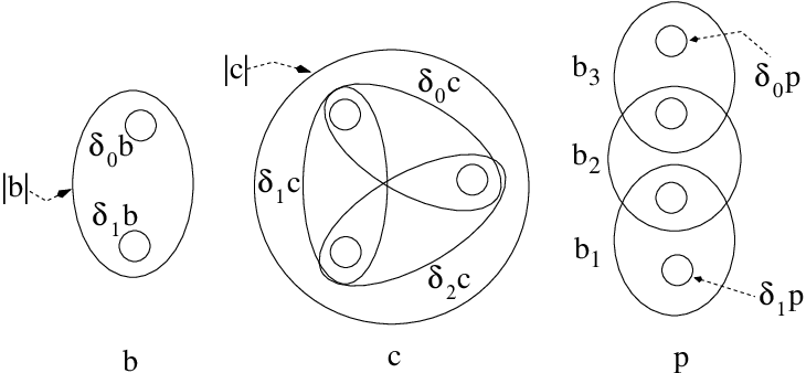
The reverse of a -simplex is the -simplex defined by
Finally, a -simplex is said to be degenerate to a -simplex whenever
We will denote by the -simplex degenerate to .
Paths
Given a pair , of -simplices a path from to is a finite ordered sequence of -simplices with the relations
The starting point of , , is the -simplex , while the endpoint of , , is the -simplex . We denote by the set of paths from to . The poset is said to be pathwise-connected if for any pair , of -simplices. The set of paths is equipped with the following operations: Consider a path . Its reverse, , is the path
The composition of with a path of is defined as
Note that forming the reverse is an involutive mapping, while the composition is associative.
4.2.2 The First Homotopy Group of a Poset
The logical steps necessary to define the first homotopy group of posets are the same as in the case of topological spaces. We first recall the definition of a homotopy of paths. Then we prove that the reverse of a path and the composition of paths are well-behaved mappings under the homotopy equivalence relation. Finally, the first homotopy group of a poset is defined.
An elementary deformation of a path consists in replacing a -simplex of the path by a pair, , , where is a singular -simplex in , or, conversely, in replacing a consecutive pair , of -simplices of by a single -simplex .

Two paths with the same endpoints are homotopic if they can be obtained from one another by a finite number of elementary deformations. Homotopy thus defines an equivalence relation on the set of paths with the same end points.
The reverse and the composition of paths are compatible with the homotopy equivalence relation. To be precise, for any , and , , we have
| (4.3a) | ||||
| (4.3b) | ||||
Furthermore, for any , the following relations hold:
| (4.4a) | ||||
| (4.4b) | ||||
where is the -simplex degenerate to .
We now are in a position to define the first homotopy group of a poset. Fix a base -simplex and consider the set of closed paths . Note that the composition and the reverse are internal operations of and that . We define
| (4.5) |
where is the homotopy equivalence relation. Let denote the homotopy class of an element of . We equip with the product
The operation is associative, and it easily follows from previous results that endowed with is a group. The identity of the group is and the inverse of is . Now assume that is pathwise-connected. Given a -simplex , let be a path from to . Then the map
is a group isomorphism. On the basis of these facts we give the following
Definition 4.1.
We call the first homotopy group of with base . If is pathwise-connected, we denote this group by and call it the fundamental group of . If we will say that is simply connected.
We have the following result:
Proposition 4.2.
If is directed, then is pathwise- and simply connected.
4.2.3 Net Cohomology of a Poset
We introduce the net cohomology of a poset equipped with a causal disjointness relation. Throughout it is assumed that the poset is pathwise-connected.
Causal disjointness and net of local algebras
Given a poset , a causal disjointness relation on is a symmetric binary relation on satisfying the following properties:
| (4.6a) | ||||
| (4.6b) | ||||
Given a subset , the causal complement of is the subset of defined as
Note that if , then . Now, assume that is a pathwise-connected poset equipped with a causal disjointness relation . A net of local algebras indexed by is a correspondence
associating with any a von Neumann algebra defined on a fixed Hilbert space and satisfying
where the prime denotes the commutant of the algebra. The algebra associated with the causal complement of , is the -algebra generated by all the algebras with and . The net is said to be irreducible whenever, given with for any , then , .
The category of -cocycles
We refer the reader to [64] for the definition of a -category. Let be a poset with a causal disjointness relation , and let be an irreducible net of local algebras. A -cocycle of with values in is a field of unitary operators satisfying the -cocycle identity,
and the locality condition, , for any -simplex . An intertwiner between a pair of -cocycles and is a field satisfying the relation
and the locality condition, , for any -simplex . The category of -cocycles is the category whose objects are -cocycles and whose arrows are the corresponding intertwiners. The composition between and is the arrow defined as
Note that the arrow of defined as for any is the identity of . It turns out that is a -category (for details cf. [102]). Two -cocycles and are equivalent (or cohomologous) if there exists a unitary arrow . A -cocycle is trivial if it is equivalent to the identity cocycle defined as for any -simplex . Note that, since is irreducible, is irreducible: .
Equivalence in and path independence
A weaker form of equivalence between -cocycles is the following. and are said to be equivalent in if there exists a field of unitary operators such that
Note that the field is not an arrow of because it is not required that satisfies the locality condition. A -cocycle is trivial in if it is equivalent in to the trivial -cocycle . We denote by the set of -cocycles that are trivial in , and with the same symbol we denote the full -subcategory of whose objects are the -cocycles trivial in . Triviality in is related to the notion of path independence. The evaluation of a -cocycle on a path is defined as
is said to be path-independent whenever
| (4.7) |
As is pathwise-connected, a -cocycle is trivial in if and only if it is path-independent [65].
Connection between homotopy and net cohomology
Let us consider a poset equipped with a causal disjointness relation , and let be an irreducible net of local algebras. In this section we establish the relation between and the set .
To begin with, note that -cocycles are invariant for homotopic paths. This means that, given and two paths , with the same endpoints,
| (4.8) |
This is easily seen because -cocycles are invariant for elementary deformations and homotopic paths are finite sequences of elementary deformations of each other. Furthermore, by invariance of -cocycles for homotopic paths and by relations (4.3) and (4.4), it turns out that
| (4.9a) | ||||
| (4.9b) | ||||
We are now in the position to show the connection between the fundamental group of and .
Theorem 4.3.
Given and a -simplex , define
| (4.10) |
Then, is a unitary representation of in . The correspondence maps -cocycles equivalent in into equivalent unitary representations of in . Up to equivalence, this map is injective. If , then .
Proof.
Observe that the definition is well-posed as is invariant for homotopic paths. By (4.9a) and (4.8)), we have , , and . Hence is a unitary representation of in . Furthermore, if and is unitary, then . So what remains to be proved is that the correspondonce is injective up to equivalence. To this end consider a unitary representation of on . For any -simplex denote by a path with and . Let
Given a -simplex , we have
Hence satisfies the -cocycle identity but in general because does not have to belong to . However, note that if we consider for some , then
Therefore, is equivalent in to . This entails that, if is equivalent to , then is equivalent in to . Finally, assume that , then for any closed path . Thus is path-independent on , hence is trivial in . ∎
Change of Index Set
We now study the behaviour of net cohomology under a change of the index set. By a subposet of a poset we mean a subset of equipped with the same order relation as .
Definition 4.4.
Consider a subposet of . We will say that is a refinement of , if for any there exists such that . A refinement of is said to be locally relatively connected if, given , for any pair , with , there is a path in from to such that .
Let be a pathwise-connected poset and let be a causal disjointness relation for . Let be an irreducible net of local algebras indexed by and defined on a Hilbert space . If is a locally relatively connected refinement of , then it is easily seen that is pathwise-connected and that is a causal disjointness relation on . Furthermore, the restriction of to is a net of local algebras indexed by . Let be the category of -cocycles of , trivial in , with values in the net . Notice that need not be irreducible. However, as is a refinement of , the trivial -cocycle of is irreducible.
Theorem 4.5.
Let be a locally relatively connected refinement of . Then the categories and are equivalent.
Proof.
For any and for any define
is a covariant and faithful functor from into . We now define a functor from to . To this end, choose a function satisfying the following properties: given , then for , otherwise . For any we denote by a path of from to whose support is contained in ; this is possible because is a locally relatively connected refinement of . Given and define
for any -simplex . As is path-independent, given , we have
Hence satisfies the -cocycle identity, and it is trivial in because so is . Therefore, . In an analogous fashion one can show that . Hence, is a covariant functor from to . Finally, it can easily be checked that the pair , constitutes an equivalence between and (for details cf. [25]). ∎
4.2.4 The Poset as a Basis for a Topological Space
Consider a topological Hausdorff space . The topics of the previous sections are now investigated in the case that is a basis for the topology of ordered under inclusion . This allows us both to show the connection between the notions for posets and the corresponding topological ones and to understand how topology affects net cohomology.
Homotopy
In what follows, by a curve in we mean a continuous function from the interval into . We recall that the reverse of a curve is the curve defined as for . If is a curve such that , the composition is the curve
Finally, the constant curve is the curve for any .
Definition 4.6.
Given a curve . A path is said to be a poset approximation of (or simply an approximation) if there is a partition of the interval such that (Fig. 4.3)
By we denote the set of approximations of .

Since is a basis for the topology of , for any curve . The converse, i. e., that for a given path there is a curve such that is an approximation of , holds if the elements of are arcwise-connected sets of the topological space . The approximations of curves have the following properties:
| (4.11a) | ||||
| (4.11b) | ||||
where , . As already said, we can find an approximation for any curve .
We now compare the connectedness relations of with those of . If the elements of are arcwise-connected sets of , then an open set is arcwise-connected in if and only if the poset , defined as
| (4.12) |
is pathwise-connected. Note that the set is a sieve of , i. e. a subfamily of such that, if and , then . Now, assume that is a sieve of . Then is pathwise-connected in if and only if the open set , defined as
| (4.13) |
is arcwise-connected in .
For simply connectedness, assume that the elements of are arcwise- and simply connected subsets of . Given two curves and with the same endpoints, let and have the same endpoints. Then
| (4.14) |
By using this approximation result we get
Theorem 4.7.
Let be a Hausdorff, arcwise-connected topological space. Assume that there is a basis for the topology of whose elements are arcwise- and simply connected subsets of . Then .
Proof.
Corollary 4.8.
Let and be as in the previous theorem. If is not simply connected, then is not directed under inclusion.
Net cohomology
The aim here is to apply the results of the previous section to the case where the topological space is a globally hyperbolic spacetime . In particular we will consider the set of globally hyperbolic regions and the set of diamonds introduced in Section 2.1. As seen there, both of them are bases for the topology of consisting of arcwise-connected elements. However, while diamonds are simply connected, this is not true for globally hyperbolic regions. So we conclude:
Proposition 4.9.
For any the following assertions hold.
- (i)
The fundamental group of and that of the poset are isomorphic.
- (ii)
The fundamental group of the poset is trivial.
So the poset does not encode the global topological features of .
We now turn to the cohomological consequences. First, note that is a locally relatively connected refinement of , since the elements of are arcwise-connected and is a basis for the topology of . Consider an irreducible net of local algebras defined on a Hilbert space , and denote by the restriction of to the set of diamonds . It is easy to check that is irreducible.
Proposition 4.10.
The following assertions hold.
- (i)
If is simply connected, then .
- (ii)
for any spacetime .
- (iii)
is equivalent to .
Proof.
Some observations are in order at this point.
- (A)
The main difference between the net cohomology of and that of is that in the former case there may exist -cocycles which are not trivial in . Examples of this kind of -cocycles arise in -dimensional chiral conformal quantum field theories [62].
- (B)
4.3 DHR and Local Covariance
Charged superselection sectors in Minkowski space are the unitary equivalence classes of irreducible representations of a net of local observables which are “local excitations” of the vacuum representation. We can distinguish two types of charged sectors according to the class of regions in spacetime which are used as index sets of the net. On the one hand, charged sectors of Doplicher-Haag-Roberts type, where one considers double cones of , and, on the other hand, charges of Buchholz-Fredenhagen type associated with a particular class of noncompact regions like spacelike cones. In both cases, sectors define a -category in which the charge structure manifests itself by the existence of a tensor product, a permutation symmetry and a conjugation(see Subsection 4.1.1).
The Reference State Space
Our aim is to study the superselection sectors of Doplicher-Haag-Roberts type in the framework of a locally covariant quantum field theory defined via the functor . The first step is to introduce the notion of a reference state space taking on the role of the vacuum representation. To this end, note that the vacuum representation serves as a reference representation that singles out charged sectors, and that it is enough to consider a vacuum representation that has the Borchers property and satisfies Haag duality11 1 It is possible to attenuate the Borchers property [101]. Conversely, up to now, for the theory of superselection sectors Haag duality or a weaker form of it [98] seems to be an essential requirement that the vacuum representation has to meet. [51].
Definition 4.11.
We call a reference state space for a locally quasi-equivalent state space on globally hyperbolic regions such that for any there is a state such that
- (a)
the net satisfies the Borchers property;
- (b)
the net , indexed by diamonds, is irreducible and satisfies punctured Haag duality.
Let us briefly explain the meaning of this definition. Given , the net satisfies the Borchers property if, given a set for any diamond with and a nonzero orthogonal projection of , there exists an isometry such that . The net satisfies punctured Haag duality if for any and for any diamond with we have
| (4.15) |
It is clear that punctured Haag duality entails Haag duality. If is irreducible and satisfies punctured Haag duality then it is locally definite, i. e., for any we have
| (4.16) |
As is a basis for the topology of , the net is locally definite as well. An example of a locally covariant quantum field theory with a state space satisfying the properties of Definition 4.11 is provided by the Klein-Gordon scalar field and by the space of quasi-free states satisfying the microlocal spectrum condition [23, 103]. We stress that we require the existence for any of at least one state satisfying punctured Haag duality. This property seems to be the correct generalization of Haag duality to deal with the nontrivial topology of arbitrary globally hyperbolic spacetimes [102]. The reason for punctured Haag duality to be assumed for the net indexed by is that contains elements which are not simply connected as well as elements whose causal complement is not arcwise-connected. Therefore, punctured Haag duality (and also Haag duality) might not hold for a net indexed by (cf. [103]).
Let us consider the main properties of such a state space.
First, as a consequence of local quasi-equivalence, for any pair , the nets and are isomorphic, i. e., there is a collection
| (4.17) |
consisting of ∗-isomorphisms of von Neumann algebras which are compatible with the net structure,
| (4.18) |
It is clear that, by restricting to the set of diamonds , one gets a net isomorphism .
Second, note that in there is a state satisfying punctured Haag duality, the Borchers property and, as seen above, local definiteness. Since the Borchers property and local definiteness are local properties, the fact that for any is a net isomorphism implies that also the net satisfies the Borchers property and local definiteness.
Third, consider the mapping and the associated injective -morphism . Any state induces two different representations of . On the one hand, if is the GNS representation associated with , then is a representation of . On the other hand, by local covariance so that the GNS representation associated with is again a representation of . As noticed before, any element of for arbitrary satisfies the Borchers property and local definiteness. Using the Borchers property, it turns out that the representations and are locally quasi-equivalent (for details cf. [24]). In particular, if we define
| (4.19) |
it turns out that
| (4.20) |
is a net isomorphism, where is the restriction of to the poset .
Fourth, the net isomorphisms just introduced satisfy the following commutation relation. Given , , then
| (4.21a) | |||||
| (4.21b) | |||||
The Selection Criterion
Definition 4.12.
The charged superselection sectors of with respect to the reference state space are the unitary equivalence classes of the irreducible elements of the categories as varies in and as varies in .
Our aim is, first to understand the charge structure of sectors of the categories on a fixed spacetime background as varies in , and second to inspect the locally covariant structure of sectors. This means that we will study the connection of sectors associated with different spacetime backgrounds which are isometrically embedded.
At this point some observations concerning the definition of superselection sectors in a locally covariant quantum field theory are in order.
- (A)
The above definition of superselection sectors in terms of net cohomology is equivalent to the usual one given in terms of representations of the net of local observables which are “sharp excitations” of a reference representation. In particular, it is shown in [24] that for any spacetime and any , to any -cocycle there corresponds a unique representation (up to equivalence) of the net of local observables which is a “sharp excitation” of a representation associated with a state satisfying punctured Haag duality.
- (B)
There are several reasons why we choose to study -cocycles of the poset instead of -cocycles of . On the one hand, fits topological and causal properties of better than : The fundamental group of is the same as that of and any diamond has an arcwise-connected causal complement. These two properties belong to the key ingredients in [102] where, in the Haag-Kastler framework, the charge structure of sharply localized sectors in a fixed background spacetime has been established. On the contrary, is simply connected irrespective of the topology of (Proposition 4.9), and it has elements with a nonarcwise-connected causal complement. On the other hand, Proposition 4.10 states that there is no loss of generality in studying path-independent -cocycles of instead of those of , since the corresponding categories are equivalent. We have to mention, however, that the cited result provides an equivalence of -categories, but it does not concern the tensorial structure of the categories. This topic is analysed in [25], where a symmetric tensor equivalence between the categories associated with and is given.
- (C)
4.3.1 Fixed Spacetime Background
In the present subsection we investigate the charge structure of superselection sectors in a fixed spacetime background . We start with the remark that for a state satisfying punctured Haag duality the corresponding category has a tensor product and a permutation symmetry and that its objects with finite statistics have conjugates. Afterwards, we will show that all the constructions can coherently be extended to the categories for any . We conclude by studying the behaviour of these categories under restriction to subregions of .
Independence of the choice of reference states
As a starting point, we apply the results of the analysis of sharply localized sectors on a fixed spacetime background , carried out in the Haag-Kastler framework, to our present setting. In particular we have
Theorem 4.13 ([102]).
Let satisfy punctured Haag duality. Then
- (i)
has a tensor product and a permutation symmetry;
- (ii)
the category has left inverses and a notion of statistics of objects;
- (iii)
the objects with finite statistics have conjugates.
The existence of at least one state satisfying punctured Haag duality for any is a cornerstone for our analysis. In fact, the tensor product and the permutation symmetry of can be extended to the category for any state by means of the net isomorphism introduced in the previous subsection. All these categories turn out to be symmetric tensor ∗-isomorphic [24]. In this review we do not consider in detail the tensor structure, but will prove that all the categories are ∗-isomorphic.
Given any pair , , consider
the net isomorphism (4.17). We stress that, in spite of our considering the categories associated with the set , the fact that is a net isomorphism of the nets indexed by is of crucial importance to establish the claimed isomorphism. Given any pair , and , define
| (4.22a) | |||||
| (4.22b) | |||||
The purpose is to show that is a ∗-isomorphism of -categories.
Theorem 4.14.
For any the category is a (symmetric tensor) -category with left inverses. Any object with finite statistics has conjugates. For any
is a covariant (symmetric tensor) ∗-isomorphism.
Proof.
As already mentioned, we will only prove that is a ∗-isomorphism for any pair , . Given , it is clear that for any -simplex . Given a -simplex we have
Hence is a -cocycle of . If is simply connected, then, by Proposition 4.10(i), is a path-independent -cocycle. For the general case consider a closed path of with endpoint . We can find a closed path of , with endpoint and an element such that and (see [24, Lemma 4.4]). Assume that is of the form . By homotopic invariance of -cocycles, we have
where path independence of has been used. Therefore, is a path-independent -cocycle. Now, making use of (4.22), one can easily check that for any . Moreover, since is a net isomorphism, is a ∗-isomorphism. Indeed, given the functor which is associated with the net isomorphism ( the inverse of ), one can easily see that and that . ∎
We will refer to the functor as the flip functor.
Restriction to subregions
Let be an open arcwise-connected subset of , such that for any pair , the set is either empty or contained in . This property says that is a globally hyperbolic spacetime. As is isometrically embedded in and diamonds are stable under isometric embeddings (Lemma 2.4) we have
Let be the net of local algebras with indices in , obtained by restricting to . Let , then inherits from the Borchers property and the local definiteness. However, it need not be irreducible. Let be the category of path-independent -cocycles of with values in . This is a -category closed under direct sums and subobjects, and, by local definiteness, the identity cocycle is irreducible. The aim now is to show that the restriction functor , defined in Theorem 4.5, is a full and faithful covariant ∗-functor.
Let and recall that the restriction functor is defined for any , and as
Note that, if we take , then it can easily be shown that the following diagram is commutative
Therefore, if is full and faithful for a particular choice of , then it is also full and faithful for any other element .
Theorem 4.15.
is a full and faithful ∗-functor.
Proof.
In the first part of the proof we follow [99, Theorem 30.2]. As observed above, it is enough to prove the assertion in the case that satisfies punctured Haag duality. Given , , let . This means that
We want prove that there exists such that whenever . Fix , define
where is a path in from to . This definition does not depend on the chosen and on the chosen path . Moreover, for any , and
What remains to be shown is that satisfies the locality condition, i. e., for any . From now on the proof is very similar to the proof of [102, Proposition 4.19]. Let , we show that for any whose closure is causally disjoint from . Fix a -simplex of such that and . First note that we can always find such that and . Furthermore, since the causal complement of is arcwise-connected, there is a path which lies in the causal complement of . Therefore,
for any . Hence, for any and . By punctured Haag duality, . Thus, we have shown that for any -simplex with . By [102, Proposition 4.19], the proof is complete. ∎
Remark 4.16.
Two comments on Theorem 4.15 are in order.
- (A)
This is a key result. It will entail that the embedding of a sector into a different spacetime preserves the statistical properties (see Subsection 4.3.2).
- (B)
Theorem 4.15 is nothing but the cohomological version of the equivalence between local and global intertwiners, a property that the superselection sectors which are preserved in the scaling limit fulfill [38] (see also [97]). We emphasize that in the present review this equivalence arises as a natural consequence of punctured Haag duality.
4.3.2 Locally Covariant Structure of Sectors
In this subsection it is shown how the locally covariant structure of superselection sectors arises. We introduce the embedding functor which gives first important information on the covariant structure of sectors. This structure is encoded in the superselection functor to be analysed subsequently.
The embedding functor
Consider , with , and let be the -morphism associated with . Given , let be the corresponding net isomorphism (4.19). Given , and , we define the map of categories, , via
| (4.23a) | |||||
| (4.23b) | |||||
where is the -simplex of defined as , , . Then, by using Theorem 4.15, it turns out that this mapping, , is a covariant symmetric tensor ∗-functor which is full and faithful. We call the embedding functor. By (4.21), the embedding and the flip functor enjoy the following relation:
| (4.24) |
The superselection functor
We can now establish the covariant structure of superselection sectors. Let be the category, whose objects are symmetric tensor -categories and whose arrows are the full and faithful, symmetric tensor ∗-functors. According to the approach to locally covariant quantum field theory expounded in this review, the superselection sectors are expected to exhibit the structure of a functor from the category into the category . We know that the superselection sectors of any spacetime identify a family of categories within the same isomorphism class, any such category is labelled by an element of the reference state space, . Since there is no natural way to associate an element of this isomorphism class to the spacetime , varying in , we are forced to make a choice.
Given a locally covariant quantum field theory and a reference state space , let a choice of states be given by
| (4.25) |
We define a map of categories via
| (4.26) |
and call the mapping the superselection functor associated with the choice . There holds the following theorem.
Theorem 4.17.
Given a choice of states the mapping
is a contravariant functor. If is another choice of states, then the functors and are isomorphic.
Proof.
Let . Since is defined as the composition of the flip and of the embedding functor, the above discussion of the embedding functor and Theorem 4.14 imply that is a full and faithful, symmetric tensor ∗-functor. Given , by (4.24), we have
Finally, the definitions of the flip and of the embedding functors imply
so that turns out to be a contravariant functor. For the rest of the proof see [24] ∎
This result establishes the covariance of charged superselection sectors. If , then to any sector of corresponds a unique sector of with the same charge quantum numbers. To be precise, let be an irreducible object with statistical parameter , where denotes the equivalence class of . Let be the conjugate of . Then is an irreducible object of such that
Furthermore, and have the same statistics, i. e.,
Moreover,
i. e., is the conjugate sector of .
Bibliography
- 1. Alexander, H. G. (ed.): The Leibniz-Clarke Correspondence: Together With Extracts from Newton’s Principia and Opticks. Manchester: Manchester University Press, 1998
- 2. Alfsen, E. M.: Compact Convex Sets and Boundary Integrals. Berlin, Heidelberg, New York: Springer-Verlag, 1971
- 3. Alfsen, E. M., Shultz, F. W.: Geometry of State Spaces of Operator Algebras. Boston, Basel, Berlin: Birkhäuser, 2003
- 4. Araki, H.: Mathematical Theory of Quantum Fields. Oxford: Oxford University Press, 1999
- 5. Araki, H.: Einführung in die Axiomatische Quantenfeldtheorie I. Vorlesung, Eidgenössische Technische Hochschule, Zürich, Wintersemester 1961/62. Ausgearbeitet von K. Hepp und F. Riahi
- 6. Araki, H.: Einführung in die Axiomatische Quantenfeldtheorie II. Vorlesung, Eidgenössische Technische Hochschule, Zürich, Sommersemester 1962. Ausgearbeitet von W. Wyss
- 7. Araki, H., Haag, R.: Collision Cross Sections in Terms of Local Observables. Commun. Math. Phys. 4, 77–91 (1967)
- 8. Bannier, U.: On Generally Covariant Quantum Field Theory and Generalized Causal and Dynamical Structures. Commun. Math. Phys. 118, 163–170 (1988)
- 9. Bannier, U.: Intrinsic Algebraic Characterization of Space-Time Structure. Int. J. Theor. Phys. 33, 1797–1809 (1994)
- 10. Bernal, A. N., Sánchez, M.: A Note on the Extendability of Compact Hypersurfaces to smooth Cauchy Hypersurfaces. [arXiv:gr-qc/0507018]
- 11. Bernal, A. N., Sánchez, M.: On Smooth Cauchy Hypersurfaces and Geroch’s Splitting Theorem. Commun. Math. Phys. 243, 461–470 (2003)
- 12. Birkhoff, G., von Neumann, J.: The Logic of Quantum Mechanics. Ann. of Math. (2) 37, 823–843 (1936)
- 13. Borchers, H.-J.: On the Structure of the Algebra of Field Operators. Nuovo Cimento 24, 214–236 (1962)
- 14. Borchers, H.-J.: On the Use of Modular Groups in Quantum Field Theory. Ann. Inst. Henri Poincaré - Physique théorique 63, 331–382 (1995)
- 15. Borchers, H.-J.: On Revolutionizing Quantum Field Theory with Tomita’s Modular Theory. J. Math. Phys. 41, 3604–3673 (2000)
- 16. Borchers, H.-J., Haag, R., Schroer, B.: The Vacuum State in Quantum Field Theory. Nuovo Cimento 29, 148–162 (1963)
- 17. Born, M., Heisenberg, W., Jordan, P.: Zur Quantenmechanik II. Z. Phys. 35, 557–615 (1926)
- 18. Born, M., Jordan, P.: Zur Quantenmechanik. Z. Phys. 34, 858–888 (1925)
- 19. Bros, J., Buchholz, D.: Towards a Relativistic KMS-Condition. Nucl. Phys. B429, 291–318 (1994)
- 20. Brunetti, R., Fredenhagen, K.: Algebraic Approach to Quantum Field Theory. [arXiv:math-ph/0411072], to appear in Encyclopedia of Mathematical Physics
- 21. Brunetti, R., Fredenhagen, K.: Interacting Quantum Fields in Curved Space: Renormalizability of . In: Operator Algebras and Quantum Field Theory (Rome, 1996), pp. 546–563. Cambridge, MA: Internat. Press, 1997
- 22. Brunetti, R., Fredenhagen, K.: Microlocal Analysis and Interacting Quantum Field Theories: Renormalization on Physical Backgrounds. Commun. Math. Phys. 208, 623–661 (2000)
- 23. Brunetti, R., Fredenhagen, K., Verch, R.: The Generally Covariant Locality Principle – A New Paradigm for Local Quantum Field Theory. Commun. Math. Phys. 237, 31–68 (2003)
- 24. Brunetti, R., Ruzzi, G.: Superselection Sectors and General Covariance I. [arXiv:gr-qc/0511118]
- 25. Brunetti, R., Ruzzi, G.: Superselection Sectors and General Covariance II. Preprint in preparation
- 26. Buchholz, D.: Gauss’ Law and the Infraparticle Problem. Phys. Lett. B174, 331–334 (1986)
- 27. Buchholz, D.: On Particles, Infraparticles, and the Problem of Asymptotic Completeness. In: Mebkhout, M., Sénéor, R. (eds.) VIIIth International Congress on Mathematical Physics (Marseille, 1986), pp. 381–389. Singapore: World Scientific, 1987
- 28. Buchholz, D., D’Antoni, C., Longo, R.: Nuclear Maps and Modular Structures II: Applications to Quantum Field Theory. Commun. Math. Phys. 129, 115–138 (1990)
- 29. Buchholz, D., Fredenhagen, K.: Locality and the Structure of Particle States. Commun. Math. Phys. 84, 1–54 (1982)
- 30. Buchholz, D., Jacobi, P.: On the Nuclearity Condition for Massless Fields. Lett. Math. Phys. 13, 313–323 (1987)
- 31. Buchholz, D., Junglas, P.: Local Properties of Equilibrium States and the Particle Spectrum in Quantum Field Theory. Lett. Math. Phys. 11, 51–58 (1986)
- 32. Buchholz, D., Junglas, P.: On the Existence of Equilibrium States in Local Quantum Field Theory. Commun. Math. Phys. 121, 255–270 (1989)
- 33. Buchholz, D., Ojima, I., Roos, H.: Thermodynamic Properties of Non-Equilibrium States in Quantum Field Theory. Ann. Phys. (N.Y.) 297, 219–242 (2002)
- 34. Buchholz, D., Porrmann, M.: How Small is the Phase Space in Quantum Field Theory? Ann. Inst. Henri Poincaré - Physique théorique 52, 237–257 (1990)
- 35. Buchholz, D., Porrmann, M., Stein, U.: Dirac versus Wigner: Towards a Universal Particle Concept in Local Quantum Field Theory. Phys. Lett. B267, 377–381 (1991)
- 36. Buchholz, D., Wichmann, E. H.: Causal Independence and the Energy-Level Density of States in Local Quantum Field Theory. Commun. Math. Phys. 106, 321–344 (1986)
- 37. D’Antoni, C., Hollands, S.: Nuclearity, Local Quasiequivalence and Split Property for Dirac Quantum Fields in Curved Spacetime, 2004. [arXiv:math-ph/0106028 v3]
- 38. D’Antoni, C., Morsella, G., Verch, R.: Scaling Algebras for Charged Fields and Short-Distance Analysis for Localizable and Topological Charges. Ann. Henri Poincaré 5, 809–870 (2004)
- 39. DeWitt, B. S., Brehme, R. W.: Radiation Damping in a Gravitational Field. Ann. Phys. (N.Y.) 9, 220–259 (1960)
- 40. Dimock, J.: Algebras of Local Observables on a Manifold. Commun. Math. Phys 77, 219–228 (1980)
- 41. Dimock, J.: Dirac Quantum Fields on a Manifold. Trans. Amer. Math. Soc. 269, 133–147 (1982)
- 42. Dirac, P. A. M.: The Fundamental Equations of Quantum Mechanics. Proc. Phys. Soc. London, Sect. A 109, 642–653 (1925)
- 43. Dixmier, J.: Von Neumann Algebras. Amsterdam, New York, Oxford: North-Holland Publishing Co., 1981
- 44. Doplicher, S., Fredenhagen, K., Roberts, J. E.: The Quantum Structure of Spacetime at the Planck Scale and Quantum Fields. Commun. Math. Phys. 172, 187–220 (1995)
- 45. Doplicher, S., Haag, R., Roberts, J. E.: Fields, Observables and Gauge Transformations I. Commun. Math. Phys. 13, 1–23 (1969)
- 46. Doplicher, S., Haag, R., Roberts, J. E.: Fields, Observables and Gauge Transformations II. Commun. Math. Phys. 15, 173–200 (1969)
- 47. Doplicher, S., Haag, R., Roberts, J. E.: Local Observables and Particle Statistics I. Commun. Math. Phys. 23, 199–230 (1971)
- 48. Doplicher, S., Haag, R., Roberts, J. E.: Local Observables and Particle Statistics II. Commun. Math. Phys. 35, 49–85 (1974)
- 49. Doplicher, S., Longo, R.: Standard and Split Inclusions of von Neumann Algebras. Invent. Math. 75, 493–536 (1984)
- 50. Doplicher, S., Roberts, J. E.: A New Duality Theory for Compact Groups. Invent. Math. 98, 157–218 (1989)
- 51. Doplicher, S., Roberts, J. E.: Why There is a Field Algebra with a Compact Gauge Group Describing the Superselection Structure in Particle Physics. Commun. Math. Phys. 131, 51–107 (1990)
- 52. Duistermaat, J. J., Hörmander, L.: Fourier Integral Operators. II. Acta Math. 128, 183–269 (1972)
- 53. Dütsch, M., Fredenhagen, K.: A Local (Perturbative) Construction of Observables in Gauge Theories: The Example of QED. Commun. Math. Phys. 203, 71–105 (1999)
- 54. Dyson, F. J.: Missed Opportunities. Bull. Amer. Math. Soc. 78, 635–652 (1972)
- 55. Einstein, A.: Die Grundlage der allgemeinen Relativitätstheorie. Ann. Phys. (Leipzig) 49, 769–822 (1916)
- 56. Einstein, A., Grossmann, M.: Entwurf einer verallgemeinerten Relativitätstheorie und einer Theorie der Gravitation. Z. Math. Phys. 62, 225–259 (1914)
- 57. Fell, J. M. G.: The Dual Spaces of -Algebras. Trans. Amer. Math. Soc. 94, 365–403 (1960)
- 58. Fewster, C. J., Verch, R.: Stability of Quantum Systems at Three Scales: Passivity, Quantum Weak Energy Inequalities and the Microlocal Spectrum Condition. Commun. Math. Phys. 240, 329–375 (2003)
- 59. Fredenhagen, K.: On the General Theory of Quantized Fields. In: Schmüdgen, K. (ed.) Proceedings of the Xth International Congress on Mathematical Physics (Leipzig, 1991), pp. 136–152. Berlin, Heidelberg, New York: Springer-Verlag, 1992
- 60. Fredenhagen, K., Haag, R.: Generally Covariant Quantum Field Theory and Scaling Limits. Commun. Math. Phys. 108, 91–115 (1987)
- 61. Fredenhagen, K., Hertel, J.: Zwei Sätze über Kompaktheit, 1979. Unpublished manuscript
- 62. Fredenhagen, K., Rehren, K.-H., Schroer, B.: Superselection Sectors with Braid Group Statistics and Exchange Algebras. II. Geometric Aspects and Conformal Covariance. Rev. Math. Phys. (Special Issue), 113–157 (1992)
- 63. Fulling, S. A.: Aspects of Quantum Field Theory in Curved Spacetime. Cambridge: Cambridge University Press, 1989
- 64. Ghez, P., Lima, R., Roberts, J. E.: -Categories. Pacific J. Math. 120, 79–109 (1985)
- 65. Guido, D., Longo, R., Roberts, J. E., Verch, R.: Charged Sectors, Spin and Statistics in Quantum Field Theory on Curved Spacetimes. Rev. Math. Phys. 13, 125–198 (2001)
- 66. Haag, R.: On Quantum Field Theories. Dan. Mat. Fys. Medd. 29, 1–37 (1955)
- 67. Haag, R.: Quantum Field Theories with Composite Particles and Asymptotic Conditions. Phys. Rev. 112, 669–673 (1958)
- 68. Haag, R.: Local Quantum Physics. 2nd ed. Berlin, Heidelberg, New York: Springer-Verlag, 1996
- 69. Haag, R., Hugenholtz, N. M., Winnink, M.: On the Equilibrium States in Quantum Statistical Mechanics. Commun. Math. Phys. 5, 215–236 (1967)
- 70. Haag, R., Kastler, D.: An Algebraic Approach to Quantum Field Theory. J. Math. Phys. 5, 848–861 (1964)
- 71. Haag, R., Swieca, J. A.: When Does a Quantum Field Theory Describe Particles? Commun. Math. Phys. 1, 308–320 (1965)
- 72. Hawking, S. W., Ellis, G. F. R.: The Large Scale Structure of Space-Time. Cambridge: Cambridge University Press, 1975
- 73. Heisenberg, W.: Über quantentheoretische Umdeutung kinematischer und mechanischer Beziehungen. Z. Phys. 33, 879–893 (1925)
- 74. Hollands, S., Wald, R. M.: Local Wick Polynomials and Time Ordered Products of Quantum Fields in Curved Spacetime. Commun. Math. Phys. 223, 289–326 (2001)
- 75. Hollands, S., Wald, R. M.: Existence of Local Covariant Time Ordered Products of Quantum Fields in Curved Spacetime. Commun. Math. Phys. 231, 309–345 (2002)
- 76. Hörmander, L.: Fourier Integral Operators. I. Acta Math. 127 (1971)
- 77. Hörmander, L.: The Analysis of Linear Partial Differential Operators I. Berlin, Heidelberg, New York: Springer-Verlag, 2003
- 78. Jordan, P., von Neumann, J., Wigner, E.: On an Algebraic Generalization of the Quantum Mechanical Formalism. Ann. of Math. (2) 35, 29–64 (1934)
- 79. Junker, W.: Adiabatic Vacua and Hadamard States for Scalar Quantum Fields on Curved Spacetimes. Ph.D. thesis, Universität Hamburg, 1995
- 80. Junker, W.: Hadamard States, Adiabatic Vacua and the Construction of Physical States for Scalar Quantum Fields on Curved Spacetime. Rev. Math. Phys. 8, 1091–1159 (1996)
- 81. Junker, W.: Erratum to Hadamard States, Adiabatic Vacua and the Construction of Physical States for Scalar Quantum Fields on Curved Spacetime [Rev. Math. Phys. 8 (1996), 1091–1159]. Rev. Math. Phys. 14, 511–517 (2002)
- 82. Junker, W., Schrohe, E.: Adiabatic Vacuum States on General Spacetime Manifolds: Definition, Construction, and Physical Properties. Ann. Henri Poincaré 3, 1113–1181 (2002)
- 83. Kawahigashi, Y., Longo, R.: Classification of Local Conformal Nets. Case . Ann. of Math. (2) 160, 493–522 (2004)
- 84. Kay, B. S.: Quantum Fields in Curved Spacetime: Non Global Hyperbolicity and Locality. In: Doplicher, S., Longo, R., Roberts, J. E., Zsidó, L. (eds.) Conference on Operator Algebras and Quantum Field Theory (Rome, July 1996). Somerville, MA: International Press, 1997
- 85. Kay, B. S., Wald, R. M.: Theorems on the Uniqueness and Thermal Properties of Stationary, Nonsingular, Quasifree States on Spacetimes with a Bifurcate Killing Horizon. Phys. Rep. 207, 49–136 (1991)
- 86. Köhler, M.: The Stress Energy Tensor of a Locally Supersymmetric Quantum Field on a Curved Spacetime. Ph.D. thesis, Universität Hamburg, 1995. [arXiv:gr-qc/9505014]
- 87. Kubo, R.: Statistical-Mechanical Theory of Irreversible Processes. I. General Theory and Simple Applications to Magnetic and Conduction Problems. J. Phys. Soc. Japan 12, 570–586 (1957)
- 88. Landsman, N. P.: Mathematical Topics Between Classical and Quantum Mechanics. Springer-Verlag, 1998
- 89. Mac Lane, S.: Categories for the Working Mathematician. 2nd ed. New York, Berlin, Heidelberg: Springer-Verlag, 1998
- 90. Martin, P. C., Schwinger, J.: Theory of Many-Particle Systems. I. Phys. Rev. 115, 1342–1373 (1959)
- 91. O’Neill, B.: Semi-Riemannian Geometry With Applications to Relativity. New York: Academic Press, 1983
- 92. Phelps, R. R.: Lectures on Choquet’s Theorem. New York, Toronto, London, Melbourne: American Book, Van Nostrand, Reinhold, 1966
- 93. Porrmann, M.: Particle Weights and Their Disintegration I. Commun. Math. Phys. 248, 269–304 (2004)
- 94. Porrmann, M.: Particle Weights and Their Disintegration II. Commun. Math. Phys. 248, 305–333 (2004)
- 95. Radzikowski, M. J.: The Hadamard Condition and Kay’s Conjecture in (Axiomatic) Quantum Field Theory on Curved Space-Time. Ph.D. thesis, Princeton University, 1992
- 96. Reeh, H., Schlieder, S.: Bemerkungen zur Unitäräquivalenz von Lorentzinvarianten Feldern. Nuovo Cimento 22, 1051–1068 (1961)
- 97. Roberts, J. E.: Local Cohomology and Superselection Structure. Commun. Math. Phys. 51, 107–119 (1976)
- 98. Roberts, J. E.: Lectures on Algebraic Quantum Field Theory. In: Kastler, D. (ed.) The Algebraic Theory of Superselection Sectors (Palermo, 1989), pp. 1–112. River Edge, NJ: World Sci. Publishing, 1990
- 99. Roberts, J. E.: More Lectures on Algebraic Quantum Field Theory. In: Doplicher, S., Longo, R. (eds.) Noncommutative Geometry, vol. 1831 of Lecture Notes in Mathematics, pp. 263–342. Berlin, Heidelberg, New York: Springer-Verlag, 2004
- 100. Ruelle, D.: On the Asymptotic Condition in Quantum Field Theory. Helv. Phys. Acta 35, 147–163 (1962)
- 101. Ruzzi, G.: Essential Properties of the Vacuum Sector for a Theory of Superselection Sectors. Rev. Math. Phys. 15, 1255–1283 (2003)
- 102. Ruzzi, G.: Homotopy of Posets, Net-Cohomology and Superselection Sectors in Globally Hyperbolic Space-Times. Rev. Math. Phys. 17, 1021–1070 (2005)
- 103. Ruzzi, G.: Punctured Haag Duality in Locally Covariant Quantum Field Theories. Commun. Math. Phys. 256, 621–634 (2005)
- 104. Sahlmann, H., Verch, R.: Passivity and Microlocal Spectrum Condition. Commun. Math. Phys 214, 705–731 (2000)
- 105. Sato, M.: Hyperfunctions and Partial Differential Equations. In: Proceedings of the International Conference on Functional Analysis and Related Topics (Tokyo, April 1969), pp. 91–94. Tokyo: University of Tokyo Press, 1970
- 106. Sato, M.: Regularity of Hyperfunction Solution of Partial Differential Equations. In: Actes du Congrès International des Mathématiciens (Nice, 1970), vol. 2, pp. 785–794. Paris: Gauthier-Villars, 1971
- 107. Segal, I. E.: Postulates for General Quantum Mechanics. Ann. of Math. (2) 48, 930–948 (1947)
- 108. Uhlmann, A.: Über die Definition der Quantenfelder nach Wightman und Haag. Wiss. Z. Karl-Marx-Univ. Leipzig Math.-Nat. Reihe 11, 213–217 (1962)
- 109. Varadarajan, V. S.: Geometry of Quantum Theory. 2nd ed. New York, Berlin, Heidelberg, Tokyo: Springer-Verlag, 1985
- 110. Verch, R.: A Spin-Statistics Theorem for Quantum Fields on Curved Spacetime Manifolds in a Generally Covariant Framework. Commun. Math. Phys. 223, 261– –288 (2001)
- 111. Wald, R. M.: General Relativity. Chicago and London: The University of Chicago Press, 1984
- 112. Wald, R. M.: Quantum Field Theory in Curved Spacetime and Black Hole Thermodynamics. Chicago and London: The University of Chicago Press, 1994
- 113. Wightman, A. S., Gårding, L.: Fields as Operator-Valued Distributions in Relativistic Quantum Theory. Ark. Fys. 28, 129–184 (1964)
- 114. Wigner, E. P.: On Unitary Representations of the Inhomogeneous Lorentz Group. Ann. of Math. (2) 40, 149–204 (1939)