Geometry of Integrable Billiards and Pencils of Quadrics

Vladimir Dragović Milena Radnović Note: on leave at The Weizmann Institute of Science, Rehovot, Israel Affiliation: Mathematical Institute SANU, Belgrade, Serbia and Montenegro Affiliation: vladad@mi.sanu.ac.yu, milena@mi.sanu.ac.yu

Abstract

We study the deep interplay between geometry of quadrics in $d$ -dimensional space and the dynamics of related integrable billiard systems. Various generalizations of Poncelet theorem are reviewed. The corresponding analytic conditions of Cayley’s type are derived giving the full description of periodical billiard trajectories; among other cases, we consider billiards in arbitrary dimension $d$ with the boundary consisting of arbitrary number $k$ of confocal quadrics. Several important examples are presented in full details demonstrating the effectiveness of the obtained results. We give a thorough analysis of classical ideas and results of Darboux and methodology of Lebesgue, and prove their natural generalizations, obtaining new interesting properties of pencils of quadrics. At the same time, we show essential connections between these classical ideas and the modern algebro-geometric approach in the integrable systems theory.

to be published in:

Journal de Mathématiques Pures et Appliquées

1 Introduction

In his Traité des propriétés projectives des figures [34], Poncelet proved one of most beautiful and most important claims of the 19th century geometry. Suppose that two ellipses are given in the plane, together with a closed polygonal line inscribed in one of them and circumscribed about the other one. Then, Poncelet theorem states that infinitely many such closed polygonal lines exist – every point of the first ellipse is a vertex of such a polygon. Besides, all these polygons have the same number of sides. Poncelet’s proof was purely geometrical, synthetic. Later, using the addition theorem for elliptic functions, Jacobi gave another proof of the theorem [27]. Essentially, Poncelet theorem is equivalent to the addition theorem and Poncelet’s proof represents a synthetic way of deriving the group structure on an elliptic curve. Another proof, in a modern, algebro-geometrical manner, can be found in Griffiths’ and Harris’ paper [23]. There, they also gave an interesting generalization of the Poncelet theorem to the three-dimensional case, considering polyhedral surfaces both inscribed and circumscribed about two quadrics.

A natural question connected with Poncelet theorem is to find an analytical condition determining, for two given conics, if an $n$ -polygon inscribed in one and circumscribed about the second conic exists. In a short paper [10], Cayley derived such a condition, using the theory of Abelian integrals. Inspired by this paper, Lebesgue translated Cayley’s proof to the language of geometry. Lebesgue’s proof of Cayley’s condition, derived by methods of projective geometry and algebra, can be found in his book Les coniques [31]. Griffiths and Harris derived Cayley theorem by finding an analytical condition for points of finite order on an elliptic curve [24].

It is worth emphasizing that Poncelet, in fact, proved a statement that is much more general than the famous Poncelet theorem [7, 34], then deriving the latter as a corollary. Namely, he considered $n+1$ conics of a pencil in the projective plane. If there exists an $n$ -polygon with vertices lying on the first of these conics and each side touching one of the other $n$ conics, then infinitely many such polygons exist. We shall refer to this statement as Complete Poncelet theorem (CPT) and call such polygons Poncelet polygons. We are going to follow here mostly the presentation of Lebesgue from [31], which is, as we learned from M. Berger, quite close to one of two Poncelet’s original proofs.

A nice historical overview of the Poncelet theorem, together with modern proofs and remarks is given in [9]. Various classical theorems of Poncelet type with short modern proofs reviewed in [5], while the algebro-geometrical approach to families of Poncelet polygons via modular curves is given in [6, 28].

Poncelet theorem has a nice mechanical interpretation. Elliptical billiard [30] is a dynamical system where a material point of the unit mass is moving with a constant velocity inside an ellipse and obeying the reflection law at the boundary, i.e. having congruent impact and reflection angles with the tangent line to the ellipse at any bouncing point. It is also assumed that the reflection is absolutely elastic. It is well known that any segment of a given elliptical billiard trajectory is tangent to the same conic, confocal with the boundary [11]. If a trajectory becomes closed after $n$ reflections, then Poncelet theorem implies that any trajectory of the billiard system, which shares the same caustic curve, is also periodic with the period $n$ .

Complete Poncelet theorem also has a mechanical meaning. The configuration dual to a pencil of conics in the plane is a family of confocal second order curves [4]. Let us consider the following, a little bit unusual billiard. Suppose $n$ confocal conics are given. A particle is bouncing on each of these $n$ conics respectively. Any segment of such a trajectory is tangent to the same conic confocal with the given $n$ curves. If the motion becomes closed after $n$ reflections, then, by Complete Poncelet theorem, any such a trajectory with the same caustic is also closed.

The statement dual to Complete Poncelet theorem can be generalized to the $d$ -dimensional space [11]. Suppose vertices of the polygon $x_{1}x_{2}\dots x_{n}$ are respectively placed on confocal quadric hyper-surfaces $\mathcal{Q}_{1}$ , $\mathcal{Q}_{2}$ , …, $\mathcal{Q}_{n}$ in the $d$ -dimensional Eucledean space, with consecutive sides obeying the reflection law at the corresponding hyper-surface. Then all sides are tangent to some quadrics $\mathcal{Q}^{1}$ , …, $\mathcal{Q}^{d-1}$ confocal with $\{\mathcal{Q}_{i}\}$ ; for the hyper-surfaces $\{\mathcal{Q}_{i},\mathcal{Q}^{j}\}$ , an infinite family of polygons with the same properties exist.

But, more than one century before these quite recent results, Darboux proved the generalization of Poncelet theorem for a billiard within an ellipsoid in the three-dimensional space [13]. It seems that his work on this topic is completely forgot nowadays.

It is natural to search for a Cayley-type condition related to some of generalizations of Poncelet theorem. The authors derived such conditions for the billiard system inside an ellipsoid in the Eucledean space of arbitrary finite dimension [19, 20]. In our recent note [21], algebro-geometric conditions for existence of periodical billiard trajectories within $k$ quadrics in $d$ -dimensional Euclidean space were announced. The aim of the present paper is to give full explanations and proofs of these results together with several important examples and improvements. The second important goal of this paper is to offer a thorough historical overview of the subject with a special attention on the detailed analysis of ideas and contributions of Darboux and Lebesgue. While Lebesgue’s work on this subject has been, although rarely, mentioned by experts, on the other hand, it seems to us that relevant Darboux’s ideas are practically unknown in the contemporary mathematics. We give natural higher dimensional generalizations of the ideas and results of Darboux and Lebesgue, providing the proofs also in the low-dimensional cases if they were omitted in the original works. Beside other results, interesting new properties of pencils of quadrics are established – see Theorems 9 and 10. The latter gives a nontrivial generalization of the Basic Lemma.

This paper is organized as follows. In the next section, a short review of Lebesgue’s results from [31] is given, followed by their application to the case of the billiard system between two confocal ellipses. Section 3 contains algebro-geometric discussions which will be applied in the rest of the paper. In Section 4, we give analytic conditions for periodicity of billiard motion inside a domain bounded by several confocal quadrics in the Euclidean space of arbitrary dimension. The complexity of the problem of billiard motion within several quadrics is well known, even in the real case, and it is induced by multivaluedness of the billiard mapping. Thus, to establish a correct setting of the problem, we introduce basic notions of reflections from inside and from outside a quadric hyper-surface, and we define the billiard ordered game. The corresponding closeness conditions are derived, together with examples and discussions. In Section 5, we consider the elliptical billiard as a discrete-time dynamical system, and, applying the Veselov’s and Moser’s algebro-geometric integration procedure, we derive the periodicity conditions. The obtained results are compared with those from Section 4. In Section 6, we give an algebro-geometric description of periodical trajectories of the billiard motion on quadric hyper-surfaces, we study the behaviour of geodesic lines after the reflection at a confocal quadric and derive a new porism of Poncelet type. In Section 7, we define the virtual reflection configuration, prove Darboux’s statement on virtual billiard trajectories, generalize it to arbitrary dimension and study related geometric questions. In Section 8, we formulate and prove highly nontrivial generalization of the Basic Lemma (Lemma 1), giving a new important geometric property of dual pencils of quadrics. In that section, we also introduce and study the generalized Cayley curve, a natural higher-dimensional generalization of the Cayley cubic studied by Lebesgue. In this way, in Section 8 the most important tools of Lebesgue’s study are generalized. Further development of this line will be presented in separate publication [22]. In Appendix 1, we review some known classes of integrable potential perturbations of elliptical billiards, emphasizing connections with Appell hypergeometric functions and Liouville surfaces. Finally, in Appendix 2, we present the related Darboux’s results considering a generalization of Poncelet theorem to Liouville surfaces, giving a good basis for a study of the geometry of periodic trajectories appearing in the perturbed systems from Appendix 1.

2 Planar Case: $d=2$ , $k$ – Arbitrary

First of all, we consider the billiard system within $k$ confocal ellipses in the 2-dimensional plane. In such a system, the billiard particle bounces sequentially of these confocal ellipses. We wish to get the analytical description of periodical trajectories of such a system.

Following Lebesgue, let us consider polygons inscribed in a conic $\Gamma$ , whose sides are tangent to $\Gamma_{1},\dots,\Gamma_{k}$ , where $\Gamma,\Gamma_{1},\dots,\Gamma_{k}$ all belong to a pencil of conics. In the dual plane, such polygons correspond to billiard trajectories having caustic $\Gamma^{*}$ with bounces on $\Gamma_{1}^{*},\dots,\Gamma_{k}^{*}$ . The main object of Lebesgue’s analysis is the cubic Cayley curve, which parametrizes contact points of tangents drawn from a given point to all conics of the pencil.

2.1 Full Poncelet Theorem

Basic Lemma. Next lemma is the main step in the proof of full Poncelet theorem. If one Poncelet polygon is given, this lemma enables us to construct every Poncelet polygon with given initial conditions. Also, the lemma is used in deriving of a geometric condition for the existence of a Poncelet polygon.

Lemma 1

[31] Let $\mathcal{F}$ be a pencil of conics in the projective plane and $\Gamma$ a conic from this pencil. Then there exist quadrangles whose vertices $A$ , $B$ , $C$ , $D$ are on $\Gamma$ such that three pairs of its non-adjacent sides $AB$ , $CD$ ; $AC$ , $BD$ ; $AD$ , $BC$ are tangent to three conics of $\mathcal{F}$ . Moreover, the six contact points all lie on a line $\Delta$ . Any such a quadrangle is determined by two sides and the corresponding contact points.

Let $\Gamma$ , $\Gamma_{1}$ , $\Gamma_{2}$ , $\Gamma_{3}$ be conics of a pencil and $ABC$ a Poncelet triangle corresponding to these conics, such that its vertices lie on $\Gamma$ and sides $AB$ , $BC$ , $CA$ touch $\Gamma_{1}$ , $\Gamma_{2}$ , $\Gamma_{3}$ respectively. This lemma gives us a possibility to construct triangle $ABD$ inscribed in $\Gamma$ whose sides $AB$ , $BD$ , $DA$ touch conics $\Gamma_{1}$ , $\Gamma_{3}$ , $\Gamma_{2}$ respectively. In a similar fashion, for a given Poncelet polygon, we can, applying Lemma 1, construct another polygon which corresponds to the same conics, but its sides are tangent to them in different order.

Circumscribed and Tangent Polygons. Let a triangle $ABC$ be inscribed in a conic $\Gamma$ and sides $BC$ , $AC$ , $AB$ touch conics $\Gamma_{1}$ , $\Gamma_{2}$ , $\Gamma_{3}$ of the pencil $\mathcal{F}$ at points $M$ , $N$ , $P$ respectively. According to the Lemma, there are two possible cases: either points $M$ , $N$ , $P$ are collinear, when we will say that the triangle is tangent to $\Gamma_{1}$ , $\Gamma_{2}$ , $\Gamma_{3}$ ; or the line $MN$ is intersecting $AB$ at a point $S$ which is a harmonic conjugate to $P$ with respect to the pair $A$ , $B$ , then we say that the triangle is circumscribed about $\Gamma_{1}$ , $\Gamma_{2}$ , $\Gamma_{3}$ .

Let $ABCD\dots KL$ be a polygon inscribed in $\Gamma$ whose sides touch conics $\Gamma_{1}$ , …, $\Gamma_{n}$ of the pencil $\mathcal{F}$ respectively. Denote by $(AC)$ a conic such that $\triangle ABC$ is circumscribed about $\Gamma_{1}$ , $\Gamma_{2}$ , $(AC)$ , by $(AD)$ a conic such that $\triangle ACD$ is circumscribed about $(AC)$ , $\Gamma_{3}$ , $(AD)$ . Similarly, we find conics $(AE)$ , …, $(AK)$ . The triangle $AKL$ can be tangent to the conics $(AK)$ , $\Gamma_{n-1}$ , $\Gamma_{n}$ or circumscribed about them, and we will say that $ABCD\dots KL$ is tangent or, respectively, circumscribed about conics $\Gamma_{1}$ , …, $\Gamma_{n}$ .

Further, we will be interested only in circumscribed polygons. The Poncelet theorem does not hold for tangent triangles nor, hence, for tangent polygons with greater number of vertices.

Theorem 1

(Complete Poncelet theorem) Let conics $\Gamma$ , $\Gamma_{1}$ , …, $\Gamma_{n}$ belong to a pencil $\mathcal{F}$ . If a polygon inscribed in $\Gamma$ and circumscribed about $\Gamma_{1}$ , …, $\Gamma_{n}$ exists, then infinitely many such polygons exist.

To determine such a polygon, it is possible to give arbitrarily:

$1)$ the order which its sides touch $\Gamma_{1}$ , …, $\Gamma_{n}$ in; let the order be: $\Gamma_{1}^{\prime}$ , …, $\Gamma_{n}^{\prime}$ ;

$2)$ a tangent to $\Gamma_{1}^{\prime}$ containing one side of the polygon;

$3)$ the intersecting point of this tangent with $\Gamma$ which will belong to the side tangent to $\Gamma_{2}^{\prime}$ .

The proof is given in [31].

2.2 Cayley’s Condition

Representation of Conics of a Pencil by Points on a Cubic Curve. Let pencil $\mathcal{F}$ of conics be determined by the curves $C=0$ and $\Gamma=0$ . The equation of an arbitrary conic of the pencil is $C+\lambda\Gamma=0$ .

Let $P+\lambda\Pi=0$ be the equation of the corresponding polar lines from the point $A\in\Gamma$ . The geometric place of contact points of tangents from $A$ with conics of the pencil is the cubic $\mathcal{C}:C\Pi-\Gamma P=0$ . On this cubic, any conic of $\mathcal{F}$ is represented by two contact points, which we will call representative points of the conic. The line determined by these two points passes through point $Z:P=0,\ \Pi=0$ . There exist exactly four conics of the pencil whose representative points coincide: the conic $\Gamma$ and three degenerate conics with representative points $A$ , $\alpha$ , $\beta$ , $\gamma$ . Lines $ZA$ , $Z\alpha$ , $Z\beta$ , $Z\gamma$ are tangents to $\mathcal{C}$ constructed from $Z$ . The tangent line to cubic $\mathcal{C}$ at point $Z$ is a polar of point $A$ with respect to the conic of the pencil which contains $Z$ .

Condition for Existence of a Poncelet Triangle. If triangles inscribed in $\Gamma$ and circumscribed about $\Gamma_{1}$ , $\Gamma_{2}$ , $\Gamma_{3}$ exist, we will say that the conics $\Gamma_{1}$ , $\Gamma_{2}$ , $\Gamma_{3}$ are joined to $\Gamma$ . In this case, CPT states there is six such triangles with the vertex $A\in\Gamma$ . Let $ABC$ be one of them. Side $AB$ , denote it by 1, touches $\Gamma_{1}$ in point $m_{1}$ . Also, it touches another conic of the pencil, denote it by $(I)$ , in point $M$ . Side $AC$ , denote it by 2’, touches $\Gamma_{2}$ in $m_{2}^{\prime}$ . Consider the quadrangle $ABCD$ determined by $AB$ , $AC$ and contact points $M$ , $m_{2}^{\prime}$ . Line $Mm_{2}^{\prime}$ meets $BC$ at $\mu_{3}$ , its point of tangency to $\Gamma_{3}$ , and meets $AD$ (which we will denote by 3’) at the point $m_{3}^{\prime}$ of tangency to $\Gamma_{3}$ . Triangle $ABD$ is circumscribed about $\Gamma_{1}$ , $\Gamma_{2}$ , $\Gamma_{3}$ .

Similarly, triangle $ACE$ can be obtained by construction of quadrangle $ABCE$ determined by $AB$ , $BC$ and contact points $m_{1}$ , $\mu_{3}$ . Line $AE$ touches $\Gamma_{3}$ at point $m_{3}\in m_{1}\mu_{3}$ . Denote this line by 3. Triangles with sides 3’, 2 and 3, 1’ are constructed analogously.

There is exactly six tangents from $A$ to conics $\Gamma_{1}$ , $\Gamma_{2}$ , $\Gamma_{3}$ . We have divided these six lines into two groups: 1,2,3 i 1’,2’,3’. Two tangents enumerated by different numbers and do not belong to the same group, determine a Poncelet triangle.

Cubic $\mathcal{C}$ and the cubic consisting of lines $m_{1}M$ , $m_{2}m_{2}^{\prime}$ , $m_{3}m_{3}^{\prime}$ have simple common points $m_{1}$ , $M$ , $m_{2}$ , $m_{2}^{\prime}$ , $m_{3}$ , $m_{3}^{\prime}$ , $A$ , and point $Z$ as a double one. A pencil determined by these two cubics contains a curve that passes through a given point of line $Mm_{2}^{\prime}$ , different from $M,m_{2}^{\prime},m_{3}^{\prime}$ . This cubic has four common points with line $Mm_{2}^{\prime}$ , so it decomposes into the line and a conic. Thus, $m_{1},m_{2},m_{3}$ are intersection points, different from $A$ and $Z$ , of a conic which contains $A$ and touches cubic $\mathcal{C}$ at $Z$ .

Converse also holds.

Let an arbitrary conic that contains point $A$ and touches cubic $\mathcal{C}$ at $Z$ be given. Denote by $m_{1}$ , $m_{2}$ , $m_{3}$ remaining intersection points of the curve $\mathcal{C}$ with this conic. Each of the lines $m_{1}Z$ , $m_{2}Z$ , $m_{3}Z$ has another common point with the cubic $\mathcal{C}$ ; denote them by $m_{1}^{\prime}$ , $m_{2}^{\prime}$ , $m_{3}^{\prime}$ respectively. By definition of the curve $\mathcal{C}$ , we have that $m_{1},m_{1}^{\prime}$ ; $m_{2},m_{2}^{\prime}$ ; $m_{3},m_{3}^{\prime}$ are pairs of representative points of some conics $\Gamma_{1}$ , $\Gamma_{2}$ , $\Gamma_{3}$ from the pencil $\mathcal{F}$ . Line $Am_{1}$ , besides being tangent to $\Gamma_{1}$ at $m_{1}$ , has to touch another conic from the pencil $\mathcal{F}$ . Take that it is tangent to a conic $(I)$ at $M$ .

Now, in a similar fashion as before, we can conclude that points $M$ , $m_{2}^{\prime}$ , $m_{3}^{\prime}$ are collinear. Applying Lemma 1, it is easily deduced that conics $\Gamma_{1}$ , $\Gamma_{2}$ , $\Gamma_{3}$ are joined to $\Gamma$ .

So, we have shown the following: systems of three joined conics are determined by systems of three intersecting points of cubic $\mathcal{C}$ with conics that contain point $A$ and touch the curve $\mathcal{C}$ at $Z$ .

Cayley’s Cubic. Let $D(\lambda)$ be the discriminant of conic $C+\lambda\Gamma=0$ . We will call the curve

\mathcal{C}_{0}:Y^{2}=D(X)

Cayley’s cubic. Representative points of conic $C+\lambda\Gamma=0$ on Cayley’s cubic are two points that correspond to the value $X=\lambda$ .

The polar conic of the point $Z$ with respect to cubic $\mathcal{C}$ passes through the contact points of the tangents $ZA$ , $Z\alpha$ , $Z\beta$ , $Z\gamma$ from $Z$ to $\mathcal{C}$ . Thus, points $\alpha,\beta,\gamma$ are representative points of three joined conics from the pencil $\mathcal{F}$ . Those three conics are obviously the decomposable ones. Corresponding values $\lambda$ diminish $D(\lambda)$ , and these three representative points on Cayley’s cubic $\mathcal{C}_{0}$ lie on the line $Y=0$ .

Using the Sylvester’s theory of residues, we will show the following:

Let three representative points of three conics of pencil $\mathcal{F}$ be given on the Cayley’s cubic $\mathcal{C}_{0}$ . Condition for these conics to be joined to the conic $\Gamma$ is that their representative points are collinear.

Sylvester’s Theory of Residues. When considering algebraic curves of genus 1, like the Cayley’s cubic is here, Abel’s theorem can always be replaced by application of this theory.

Proposition 1

Let a given cubic and an algebraic curve of degree $m+n$ meet at $3(m+n)$ points. If there is $3m$ points among them which are placed on a curve of degree $m$ , then the remaining $3n$ points are placed on a curve of degree $n$ .

If the union of two systems of points is the complete intersection of a given cubic and some algebraic curve, then we will say that these two systems are residual to each other. Now, the following holds:

Proposition 2

If systems $\mathcal{A}$ and $\mathcal{A}^{\prime}$ of points on a given cubic curve have a common residual system, then they share all residual systems.

Proof. Suppose $\mathcal{B}$ is a system residual to both $\mathcal{A}$ , $\mathcal{A}^{\prime}$ and $\mathcal{B}^{\prime}$ is residual to $\mathcal{A}$ . Then $\mathcal{A}\cup\mathcal{A}^{\prime}$ is residual to $\mathcal{B}\cup\mathcal{B}^{\prime}$ , i.e. the system $\mathcal{A}\cup\mathcal{A}^{\prime}\cup\mathcal{A}\cup\mathcal{A}^{\prime}$ is a complete intersection of the cubic with an algebraic curve. Since $\mathcal{A}\cup\mathcal{B}$ is also such an intersection, it follows, by the previous proposition, that $\mathcal{A}^{\prime}$ and $\mathcal{B}^{\prime}$ are residual to each other. $\Box$

Let us note that this proposition can be derived as a consequence of Abel’s theorem, for a plane algebraic curve of arbitrary degree. However, if the degree is equal to three, i.e. the curve is elliptic, Proposition 2 is equivalent to Abel’s theorem.

Condition for Existence of a Poncelet Polygon. Let conics $\Gamma,\Gamma_{1},\dots,\Gamma_{n}$ be from a pencil. If there exists a polygon inscribed in $\Gamma$ and circumscribed about $\Gamma_{1},\dots,\Gamma_{n}$ , we are going to say that conics $\Gamma_{1},\dots,\Gamma_{n}$ are joined to $\Gamma$ . Then, similarly as in the case of the triangle, it can be proved that tangents from the point $A\in\Gamma$ to $\Gamma_{1},\dots,\Gamma_{n}$ can be divided into two groups such that any Poncelet $n$ -polygon with vertex $A$ has exactly one side in each of the groups.

This division of tangents gives a division of characteristic points of conics $\Gamma_{1}$ , …, $\Gamma_{n}$ into two groups on $\mathcal{C}$ and, therefore, a division into two groups on Cayley’s cubic $\mathcal{C}_{0}$ : 1,2,3, …and 1’,2’,3’, ….

Let $ABCD\dots KL$ be a Poncelet polygon, and let $(AC),(AD),\dots$ be conics determined like in the definition of a circumscribed polygon. Let $c,\gamma$ ; $d,\delta$ ; …be a corresponding characteristic points on $\mathcal{C}_{0}$ , such that triples 1, 2, $c$ ; $\gamma$ , 3, $d$ ; $\delta$ , 4, $e$ are characteristic points of the same group with respect to corresponding conics.

Points 1, 2, $c$ are collinear, as $\gamma$ , 3, $d$ are. Thus, 1, 2, 3, $d$ are residual with $c,\gamma$ . Line $c\gamma$ contains point $Z$ , so system $c,\gamma$ is residual with $Z$ , too. It is possible to show that $Z$ is a triple point of curve $\mathcal{C}_{0}$ and it follows that it is residual with system $Z,Z$ . This implies that points 1,2,3, $d,Z,Z$ are placed on a conic.

If we take a coordinate system such that the tangent line to $\mathcal{C}_{0}$ at $Z$ is the infinite line and the axis $Oy$ is line $AZ$ , we will have:

four conics are joined to $\Gamma$ if and only if their characteristic points of the same group are on a parabola with the asymptotic direction $Oy$ .

Continuing deduction in the same manner, we can conclude: $3n-p$ points of the cubic $\mathcal{C}_{0}$ are characteristic points of same group for $3n-p$ conics $(1\leq p\leq 3)$ joined to $\Gamma$ , if and only if these points are placed on a curve of degree $n$ which has $Oy$ as an asymptotic line of the order $p$ .

Cayley’s Condition. Let $\mathcal{C}_{0}:y^{2}=D(x)$ be the Cayley’s cubic, where $D(x)$ is the discriminant of the conic $C+x\Gamma=0$ from pencil $\mathcal{F}$ . A system of $n$ conics joined to $\Gamma$ is determined by $n$ values $x$ if and only if these $n$ values are abscissae of intersecting points of $\mathcal{C}_{0}$ and some algebraic curve. Plugging $D(x)$ instead of $y^{2}$ in the equation of this curve, we obtain:

P(x)y+Q(x)=0,

that is

P(x)\sqrt{D(x)}+Q(x)=0.

From there:

\sqrt{D(x)}(a_{0}x^{p-2}+a_{1}x^{p-3}+\dots+a_{p-2})+(b_{0}x^{p}+b_{1}x^{p-1}+\dots+b_{p})=0,\quad n=2p;

\sqrt{D(x)}(a_{0}x^{p-1}+a_{1}x^{p-2}+\dots+a_{p-1})+(b_{0}x^{p}+b_{1}x^{p-1}+\dots+b_{p})=0,\quad n=2p+1.

If $\lambda_{1},\dots,\lambda_{k}$ denote parameters corresponding to $\Gamma_{1},\dots,\Gamma_{k}$ respectively, then existence of a Poncelet polygon inscribed in $\Gamma$ and circumscribed about $\Gamma_{1},\dots,\Gamma_{k}$ is equivalent to:

\left|\begin{array}[]{ccccccccc}1&\lambda_{1}&\lambda_{1}^{2}&\dots&\lambda_{1}^{p}&\sqrt{D(\lambda_{1})}&\lambda_{1}\sqrt{D(\lambda_{1})}&\dots&\lambda_{1}^{p-2}\sqrt{D(\lambda_{1})}\\ \dots\\ \dots\\ 1&\lambda_{k}&\lambda_{k}^{2}&\dots&\lambda_{k}^{p}&\sqrt{D(\lambda_{k})}&\lambda_{k}\sqrt{D(\lambda_{k})}&\dots&\lambda_{k}^{p-2}\sqrt{D(\lambda_{k})}\end{array}\right|=0,

for $k=2p$ ;

\left|\begin{array}[]{ccccccccc}1&\lambda_{1}&\lambda_{1}^{2}&\dots&\lambda_{1}^{p}&\sqrt{D(\lambda_{1})}&\lambda_{1}\sqrt{D(\lambda_{1})}&\dots&\lambda_{1}^{p-1}\sqrt{D(\lambda_{1})}\\ \dots\\ \dots\\ 1&\lambda_{k}&\lambda_{k}^{2}&\dots&\lambda_{k}^{p}&\sqrt{D(\lambda_{k})}&\lambda_{k}\sqrt{D(\lambda_{k})}&\dots&\lambda_{k}^{p-1}\sqrt{D(\lambda_{k})}\end{array}\right|=0,

for $k=2p+1$ .

There exists an $n$ -polygon inscribed in $\Gamma$ and circumscribed about $C$ if and only if it is possible to find coefficients $a_{0}$ , $a_{1}$ , …; $b_{0}$ , $b_{1}$ , …such that function $P(x)\sqrt{D(x)}+Q(x)$ has $x=0$ as a root of the multiplicity $n$ .

For $n=2p$ , this is equivalent to the existence of a non-trivial solution of the following system:

\begin{array}[]{ccccccccc}a_{0}C_{3}&+&a_{1}C_{4}&+&\dots&+&a_{p-2}C_{p+1}&=&0\\ a_{0}C_{4}&+&a_{1}C_{5}&+&\dots&+&a_{p-2}C_{p+2}&=&0\\ \dots\\ a_{0}C_{p+1}&+&a_{1}C_{p+2}&+&\dots&+&a_{p-2}C_{2p-1}&=&0,\end{array}

where

\sqrt{D(x)}=A+Bx+C_{2}x^{2}+C_{3}x^{3}+\dots.

Finally, for $n=2p$ , we obtain the Cayley’s condition

\left|\begin{array}[]{llll}C_{3}&C_{4}&\dots&C_{p+1}\\ C_{4}&C_{5}&\dots&C_{p+2}\\ &&\dots\\ C_{p+1}&C_{p+2}&\dots&C_{2p-1}\end{array}\right|=0.

Similarly, for $n=2p+1$ , we obtain:

\left|\begin{array}[]{llll}C_{2}&C_{3}&\dots&C_{p+1}\\ C_{3}&C_{4}&\dots&C_{p+2}\\ &&\dots\\ C_{p+1}&C_{p+2}&\dots&C_{2p}\end{array}\right|=0.

These results can be directly applied to the billiard system within an ellipse: to determine whether a billiard trajectory with a given confocal caustic is periodic, we need to consider the pencil determined by the boundary and the caustic curve.

2.3 Some Applications of Lebesgue’s Results

Now, we are going to apply the Lebesgue’s results to billiards systems within several confocal conics in the plane.

Consider the dual plane. The case with two ellipses, when the billiard trajectory is placed between them and particle bounces to one and another of them alternately, is of special interest.

Corollary 1

The condition for the existence of $2m$ -periodic billiard trajectory which bounces exactly $m$ times to the ellipse $\Gamma_{1}^{*}=C^{*}$ and $m$ times to $\Gamma_{2}^{*}=(C+\gamma\Gamma)^{*}$ , having $\Gamma^{*}$ for the caustic, is:

\det\left(\begin{array}[]{llll}f_{0}(0)&f_{1}(0)&\dots&f_{2m-1}(0)\\ f_{0}^{\prime}(0)&f_{1}^{\prime}(0)&\dots&f_{2m-1}^{\prime}(0)\\ &&\dots\\ f_{0}^{(m-1)}(0)&f_{1}^{(m-1)}(0)&\dots&f_{2m-1}^{(m-1)}(0)\\ f_{0}(\gamma)&f_{1}(\gamma)&\dots&f_{2m-1}(\gamma)\\ f_{0}^{\prime}(\gamma)&f_{1}^{\prime}(\gamma)&\dots&f_{2m-1}^{\prime}(\gamma)\\ &&\dots\\ f_{0}^{(m-1)}(\gamma)&f_{1}^{(m-1)}(\gamma)&\dots&f_{2m-1}^{(m-1)}(\gamma)\end{array}\right)=0,

where $f_{j}=x^{j}$ , $(0\leq j\leq m)$ , $f_{m+i}=x^{i-1}\sqrt{D(x)}$ , $(1\leq i\leq m-1)$ .

We consider a simple example with four bounces on each of the two conics.

Example 1

The condition on a billiard trajectory placed between ellipses $\Gamma_{1}^{*}$ and $\Gamma_{2}^{*}$ , to be closed after 4 alternate bounces to each of them is:

\det X=0,

where the elements of the $3\times 3$ matrix $X$ are:

	$\displaystyle X_{11}$	$\displaystyle=-4B_{0}+B_{1}\gamma+4C_{0}+3C_{1}\gamma+2C_{2}\gamma^{2}+C_{3}\gamma^{3}$
	$\displaystyle X_{12}$	$\displaystyle=-3B_{0}+B_{1}\gamma+3C_{0}+2C_{1}\gamma+C_{2}\gamma^{2}$
	$\displaystyle X_{13}$	$\displaystyle=-2B_{0}+B_{1}\gamma+2C_{0}+C_{1}\gamma$
	$\displaystyle X_{21}$	$\displaystyle=-6B_{0}+B_{2}\gamma^{2}+6C_{0}+6C_{1}\gamma+4C_{2}\gamma^{2}+3C_{3}\gamma^{3}$
	$\displaystyle X_{22}$	$\displaystyle=-6B_{0}+B_{1}\gamma+B_{2}\gamma^{2}+6C_{0}+4C_{1}\gamma+3C_{2}\gamma^{2}$
	$\displaystyle X_{23}$	$\displaystyle=-5B_{0}+2B_{1}\gamma+B_{2}\gamma^{2}+5C_{0}+3C_{1}\gamma$
	$\displaystyle X_{31}$	$\displaystyle=-4B_{0}+B_{3}\gamma^{3}+4C_{0}+4C_{1}\gamma+4C_{2}\gamma^{2}+3C_{3}\gamma^{3}$
	$\displaystyle X_{32}$	$\displaystyle=-4B_{0}+B_{2}\gamma^{2}+B_{3}\gamma^{3}+4C_{0}+4C_{1}\gamma+3C_{2}\gamma^{2}$
	$\displaystyle X_{33}$	$\displaystyle=-4B_{0}+B_{1}\gamma+B_{2}\gamma^{2}+B_{3}\gamma^{3}+4C_{0}+3C_{1}\gamma,$

with $C_{i},B_{i}$ being coefficients in the Taylor expansions around $x=0$ and $x=\gamma$ respectively:

	$\displaystyle\sqrt{D(x)}$	$\displaystyle=C_{0}+C_{1}x+C_{2}x^{2}+\dots,$
	$\displaystyle\sqrt{D(x)}$	$\displaystyle=B_{0}+B_{1}(x-\gamma)+B_{2}(x-\gamma)^{2}+\dots.$

On Figure 2, we see a Poncelet octagon inscribed in $\Gamma$ and circumscribed about $\Gamma_{1}$ and $\Gamma_{2}$ . In the dual plane, the billiard trajectory that corresponds to this octagon, has the dual conic $\Gamma^{*}$ as the caustic (see Figure 2).

Refer to caption — Figure 1: A Poncelet octagon whose sides touch the conics $\Gamma_{1}$ and $\Gamma_{2}$ alternately

3 Points of Finite Order on the Jacobian of a Hyperelliptic Curve

In order to prepare the algebro-geometric background for the rest of the article, in this section we are going to give the analytical characterization of some classes of finite order divisors on a hyperelliptic curve.

Let the curve $\mathcal{C}$ be given by

y^{2}=(x-x_{1})\dots(x-x_{2g+1}),\quad x_{i}\neq x_{j}\ \ \text{when}\ \ i\neq j.

It is a regular hyperelliptic curve of genus $g$ , embedded in $P^{2}$ . Let $\mathcal{J}(\mathcal{C})$ be its Jacobian variety and

\mathcal{A}\ :\ \mathcal{C}\rightarrow\mathcal{J}(\mathcal{C})

the Abel-Jacobi map.

Take $E$ to be the point which corresponds to the value $x=\infty$ , and choose $\mathcal{A}(E)$ to be the neutral in $\mathcal{J}(\mathcal{C})$ . According to the Abel’s theorem [25], $\mathcal{A}(P_{1})+\dots+\mathcal{A}(P_{n})=0$ if and only if there exists a meromorphic function $f$ with zeroes $P_{1},\dots,P_{n}$ and a pole of order $n$ at the point $E$ . Let $\mathcal{L}(nE)$ be the vector space of meromorphic functions on $\mathcal{C}$ with a unique pole $E$ of order at most $n$ , and $f_{1},\dots,f_{k}$ a basis of $\mathcal{L}(nE)$ . The mapping

F:\mathcal{C}\to P^{k-1},\quad X\mapsto[f_{1}(X),\dots,f_{k}(X)]

is a projective embedding whose image is a smooth algebraic curve of degree $n$ . Hyperplane sections of this curve are zeroes of functions from $\mathcal{L}(nE)$ . Thus, the equality $n\mathcal{A}(P)=0$ is equivalent to:

\mathrm{rank}\left(\begin{array}[]{llll}f_{1}(P)&f_{2}(P)&\dots&f_{k}(P)\\ f_{1}^{\prime}(P)&f_{2}^{\prime}(P)&\dots&f_{k}^{\prime}(P)\\ &&\dots\\ f_{1}^{(n-1)}(P)&f_{2}^{(n-1)}(P)&\dots&f_{k}^{(n-1)}(P)\end{array}\right)<k.

(1)

Lemma 2

For $n\leq 2g$ , there does not exist a point $P$ on the curve $\mathcal{C}$ , such that $n\mathcal{A}(P)=0$ and $P\neq E$ .

Proof. Let $P$ be a point on $\mathcal{C}$ , $P\neq E$ , and $x=x_{0}$ its corresponding value. Consider the case of $n$ even. Since $E$ is a branch point of a hyperelliptic curve, its Weierstrass gap sequence is $1,3,5,\dots,2g-1$ [25]. Now, applying the Riemann-Roch theorem, we obtain $\dim\mathcal{L}(nE)=n/2+1$ . Choosing a basis $1,x,\dots,x^{n/2}$ for $\mathcal{L}(nE)$ , and substituting in (1), we come to a contradiction. $\Box$

Lemma 3

Let $P(x_{0},y_{0})$ be a non-branching point on the curve $\mathcal{C}$ . For $n>2g$ , equality $n\mathcal{A}(P)=0$ is equivalent to:

\mathrm{rank}\left(\begin{array}[]{llll}B_{m+1}&B_{m}&\dots&B_{g+2}\\ B_{m+2}&B_{m+1}&\dots&B_{g+3}\\ &&\dots\\ B_{2m-1}&B_{2m-2}&\dots&B_{m+g}\end{array}\right)<m-g,\quad\text{when}\ \ n=2m,

(2)

\mathrm{rank}\left(\begin{array}[]{llll}B_{m+1}&B_{m}&\dots&B_{g+1}\\ B_{m+2}&B_{m+1}&\dots&B_{g+2}\\ &&\dots\\ B_{2m}&B_{2m-1}&\dots&B_{m+g}\end{array}\right)<m-g+1,\quad\text{when}\ \ n=2m+1,

and $\sqrt{(x-x_{1})\dots(x-x_{2g+1})}=B_{0}+B_{1}(x-x_{0})+B_{2}(x-x_{0})^{2}+B_{3}(x-x_{0})^{3}+\cdots$ .

Proof. This claim follows from previous results by choosing a basis for $\mathcal{L}(nE)$ :

\hfil\displaystyle 1,x,\dots,x^{m},y,xy,\dots,x^{m-g-1}y\ \text{if}\ n=2m,

\hfil\displaystyle 1,x,\dots,x^{m},y,xy,\dots,x^{m-g}y\ \text{if}\ n=2m+1,

similarly as in [24]. $\Box$

In the next lemma, we are going to consider the case when the curve $\mathcal{C}$ is singular, i.e. when some of the values $x_{1}$ , $x_{2}$ , …, $x_{2g+1}$ coincide.

Lemma 4

Let the curve $\mathcal{C}$ be given by

y^{2}=(x-x_{1})\dots(x-x_{2g+1}),\quad x_{1}\cdot x_{2}\cdot\dots\cdot x_{2g+1}\neq 0,

$P_{0}$ one of the points corresponding to the value $x=0$ and $E$ the infinite point on $\mathcal{C}$ . Then $2nP_{0}\sim 2nE$ is equivalent to (2), where

y=\sqrt{(x-x_{1})\dots(x-x_{2g+1})}=B_{0}+B_{1}x+B_{2}x^{2}+\dots

is the Taylor expansion around the point $P_{0}$ .

Proof. Suppose that, among $x_{1},\dots,x_{2g+1}$ , only $x_{2g}$ and $x_{2g+1}$ have same values. Then $(x_{2g},0)$ is an ordinary double point on $\mathcal{C}$ . The normalization of the curve $\mathcal{C}$ is the pair $(\tilde{\mathcal{C}},\pi)$ , where $\tilde{\mathcal{C}}$ is the curve given by:

\tilde{\mathcal{C}}:\tilde{y}^{2}=(\tilde{x}-x_{1})\dots(\tilde{x}-x_{2g-1}),

and $\pi:\tilde{\mathcal{C}}\to\mathcal{C}$ is the projection:

(\tilde{x},\tilde{y})\mathrel{\mathop{\kern 0.0pt\longmapsto}\limits^{\pi}}(x=\tilde{x},\ y=(\tilde{x}-x_{2g})\tilde{y}).

The genus of $\tilde{\mathcal{C}}$ is $g-1$ .

Denote by $A$ and $B$ points on $\tilde{\mathcal{C}}$ which are mapped to the singular point $(x_{2g},0)\in\mathcal{C}$ by the projection $\pi$ . Any other point on $\mathcal{C}$ is the image of a unique point of the curve $\tilde{\mathcal{C}}$ . Let

\pi(\tilde{E})=E,\quad\pi(\tilde{P}_{0})=P_{0}.

The relation $2nP_{0}\sim 2nE$ holds if and only if there exists a meromorphic function $f$ on $\tilde{\mathcal{C}}$ , $f\in\mathcal{L}(2n\tilde{E})$ , having a zero of order $2n$ at $\tilde{P}_{0}$ and satisfying $f(A)=f(B)$ .

For $n\leq g-1$ , according to Lemma 3, $2n\tilde{E}\sim 2n\tilde{P}_{0}$ cannot hold. For $n\geq g$ , choose the following basis of the space $\mathcal{L}(2n\tilde{E})$ :

1,\ \tilde{y},\ f_{1}\circ\pi,\ \dots,\ f_{n-g-1}\circ\pi,

where $1,f_{1},\dots,f_{n-g-1}$ is a basis of $\mathcal{L}(2nE)$ as in the proof of Lemma 3.

Since $\tilde{y}$ is the only function in the basis which has different values at points $A$ and $B$ , we obtain that the condition

2n\tilde{E}\sim 2n\tilde{P}_{0}

is equivalent to (2).

Cases when $\mathcal{C}$ has more singular points or singularities of higher order, can be discussed in the same way. $\Box$

Lemma 5

Let the curve $\mathcal{C}$ be given by

y^{2}=(x-x_{1})\dots(x-x_{2g+2}),

with all $x_{i}$ distinct from $0$ , and $Q_{+}$ , $Q_{-}$ the two points on $\mathcal{C}$ over the point $x=0$ . Then $nQ_{+}\sim nQ_{-}$ is equivalent to:

\mathrm{rank}\left(\begin{array}[]{llll}B_{g+2}&B_{g+3}&\dots&B_{n+1}\\ B_{g+3}&B_{g+4}&\dots&B_{n+2}\\ \dots&\dots&\dots&\dots\\ \dots&\dots&\dots&\dots\\ \\ B_{g+n}&\dots&\dots&B_{2n-1}\end{array}\right)<n-g\quad\text{and}\quad n>g,

(3)

where $y=\sqrt{(x-x_{1})\dots(x-x_{2g+2})}=B_{0}+B_{1}x+B_{2}x^{2}+\dots$ is the Taylor expansion around the point $Q_{-}$ .

Proof. $\mathcal{C}$ is a hyperelliptic curve of genus $g$ . The relation $nQ_{+}\equiv nQ_{-}$ means that there exists a meromorphic function on $\mathcal{C}$ with a pole of order $n$ at the point $Q_{+}$ , a zero of the same order at $Q_{-}$ and neither other zeros nor poles. Denote by $L(nQ_{+})$ the vector space of meromorphic functions on $\mathcal{C}$ with a unique pole $Q_{+}$ of order at most $n$ . Since $Q_{+}$ is not a branching point on the curve, $\dim L(nQ_{+})=1$ for $n\leq g$ , and $\dim L(nQ_{+})=n-g+1$ , for $n>g$ . In the case $n\leq g$ , the space $L(nQ_{+})$ contains only constant functions, and the divisors $nQ_{+}$ and $nQ_{-}$ can not be equivalent. If $n\geq g+1$ , we choose the following basis for $L(nQ_{+})$ :

1,f_{1},\dots,f_{n-g},

where

f_{k}=\frac{y-B_{0}-B_{1}x-\dots-B_{g+k-1}x^{g+k-1}}{x^{g+k}}.

Thus, $nQ_{+}\equiv nQ_{-}$ if there is a function $f\in L(nQ_{+})$ with a zero of order $n$ at $Q_{-}$ , i.e., if there exist constants $\alpha_{0},\dots,\alpha_{n-g}$ , not all equal to 0, such that:

\begin{array}[]{ccccccccl}\alpha_{0}&+&\alpha_{1}f_{1}(Q_{-})&+&\dots&+&\alpha_{n-g}f_{n-g}(Q_{-})&=&0\\ &&\alpha_{1}f_{1}^{\prime}(Q_{-})&+&\dots&+&\alpha_{n-g}f_{n-g}^{\prime}(Q_{-})&=&0\\ &\dots\\ &\dots\\ \\ &&\alpha_{1}f_{1}^{(n-1)}(Q_{-})&+&\dots&+&\alpha_{n-g}f_{n-g}^{(n-1)}(Q_{-})&=&0.\end{array}

Existence of a non-trivial solution to this system of linear equations is equivalent to the condition (3).

When some of the values $x_{1},\dots,x_{2g+2}$ coincide, the curve $\mathcal{C}$ is singular. This case can be considered by the procedure of normalization of the curve, as in Lemma 4. The condition for the equivalence of the divisors $nQ_{+}$ i $nQ_{-}$ , in the case when $\mathcal{C}$ is singular, is again (3). $\Box$

4 Periodic Billiard Trajectories inside $k$ Confocal Quadrics in $\mathbf{R}^{\mathbf{d}}$

Darboux was the first who considered a higher-dimensional generalization of Poncelet theorem. Namely, he investigated light-rays in the three-dimensional case ( $d=3$ ) and announced the corresponding complete Poncelet theorem in [13] in 1870.

Higher-dimensional generalizations of CPT ( $d\geq 3$ ) were obtained quite recently in [11], and the related Cayley-type conditions were derived by the authors [21].

The main goal of this section is to present detailed proof of Cayley-type condition for generalized CPT, together with discussions and examples.

Consider an ellipsoid in ${\mathbb{R}}^{d}$ :

\frac{x_{1}^{2}}{a_{1}}+\dots+\frac{x_{d}^{2}}{a_{d}}=1,\quad a_{1}>\dotsb>a_{d}>0,

and the related system of Jacobian elliptic coordinates $(\lambda_{1},\dots,\lambda_{d})$ ordered by the condition

\lambda_{1}>\lambda_{2}>\dotsb>\lambda_{d}.

If we denote:

Q_{\lambda}(x)=\frac{x_{1}^{2}}{a_{1}-\lambda}+\dots+\frac{x_{d}^{2}}{a_{d}-\lambda},

then any quadric from the corresponding confocal family is given by the equation of the form:

\mathcal{Q}_{\lambda}:\ Q_{\lambda}(x)=1.

(4)

The famous Chasles theorem states that any line in the space $\mathbb{R}^{d}$ is tangent to exactly $d-1$ quadrics from a given confocal family. Next lemma gives an important condition on these quadrics.

Lemma 6

Suppose a line $\ell$ is tangent to quadrics $\mathcal{Q}_{\alpha_{1}},\dots,\mathcal{Q}_{\alpha_{d-1}}$ from the family (4). Then Jacobian coordinates $(\lambda_{1},\dots,\lambda_{d})$ of any point on $\ell$ satisfy the inequalities $\mathcal{P}(\lambda_{s})\geq 0$ , $s=1,\dots,d$ , where

\mathcal{P}(x)=(a_{1}-x)\dots(a_{d}-x)(\alpha_{1}-x)\dots(\alpha_{d-1}-x).

Proof. Let $x$ be a point of $\ell$ , $(\lambda_{1},\dots,\lambda_{d})$ its Jacobian coordinates, and $y$ a vector parallel to $\ell$ . The equation $Q_{\lambda}(x+ty)=1$ is quadratic with respect to $t$ . Its discriminant is:

\Phi_{\lambda}(x,y)=Q_{\lambda}(x,y)^{2}-Q_{\lambda}(y)\bigl(Q_{\lambda}(x)-1\bigr),

where

Q_{\lambda}(x,y)=\frac{x_{1}y_{1}}{a_{1}-\lambda}+\dots+\frac{x_{d}y_{d}}{a_{d}-\lambda}.

By [33],

\Phi_{\lambda}(x,y)=\frac{(\alpha_{1}-\lambda)\dots(\alpha_{d-1}-\lambda)}{(a_{1}-\lambda)\dots(a_{d}-\lambda)}.

For each of the coordinates $\lambda=\lambda_{s}$ , ( $1\leq s\leq d$ ), the quadratic equation has a solution $t=0$ ; thus, the corresponding discriminants are non-negative. This is obviously equivalent to $\mathcal{P}(\lambda_{s})\geq 0$ . $\Box$

4.1 Billiard inside a Domain Bounded by Confocal Quadrics

Suppose that a bounded domain $\Omega\subset\mathbb{R}^{d}$ is given such that its boundary $\partial\Omega$ lies in the union of several quadrics from the family (4). Then, in elliptic coordinates, $\Omega$ is given by:

\beta_{1}^{\prime}\leq\lambda_{1}\leq\beta_{1}^{\prime\prime},\quad\dots,\quad\beta_{d}^{\prime}\leq\lambda_{d}\leq\beta_{d}^{\prime\prime},

where $a_{s+1}\leq\beta_{s}^{\prime}<\beta_{s}^{\prime\prime}\leq a_{s}$ for $1\leq s\leq d-1$ and $-\infty<\beta_{d}^{\prime}<\beta_{d}^{\prime\prime}\leq a_{d}$ .

Consider a billiard system within $\Omega$ and let $\mathcal{Q}_{\alpha_{1}}$ , …, $\mathcal{Q}_{\alpha_{d-1}}$ be caustics of one of its trajectories. For any $s=1,\dots,d$ , the set $\Lambda_{s}$ of all values taken by the coordinate $\lambda_{s}$ on the trajectory is, according to Lemma 6, included in $\Lambda_{s}^{\prime}=\{\,\lambda\in[\beta_{s}^{\prime},\beta_{s}^{\prime\prime}]\,:\,\mathcal{P}(\lambda)\geq 0\,\}$ . By [29], each of the intervals $(a_{s+1},a_{s})$ , $(2\leq s\leq d)$ contains at most two of the values $\alpha_{1},\dots,\alpha_{d-1}$ , the interval $(-\infty,a_{d})$ contains at most one of them, while none is included in $(a_{1},+\infty)$ . Thus, for each $s$ , the following three cases are possible:

First case: $\alpha_{i},\alpha_{j}\in[\beta_{s}^{\prime},\beta_{s}^{\prime\prime}]$ , $\alpha_{i}<\alpha_{j}$ . Since any line which contains a segment of the trajectory touches $\mathcal{Q}_{\alpha_{i}}$ and $\mathcal{Q}_{\alpha_{j}}$ , the whole trajectory is placed between these two quadrics. The elliptic coordinate $\lambda_{s}$ has critical values at points where the trajectory touches one them, and remains monotonous elsewhere. Hence, meeting points with with $\mathcal{Q}_{\alpha_{i}}$ and $\mathcal{Q}_{\alpha_{j}}$ are placed alternately along the trajectory and $\Lambda_{s}=\Lambda_{s}^{\prime}=[\alpha_{i},\alpha_{j}]$ .

Second case: Among $\alpha_{1},\dots,\alpha_{d-1}$ , only $\alpha_{i}$ is in $[\beta_{s}^{\prime},\beta_{s}^{\prime\prime}]$ . $\mathcal{P}$ is non-negative in exactly one of the intervals: $[a_{s+1},\alpha_{i}]$ , $[\alpha_{i},a_{s}]$ , let us take in the first one. Then the trajectory has bounces only on $\mathcal{Q}_{\beta_{s}^{\prime}}$ . If $\alpha_{i}\neq\beta_{s}^{\prime\prime}$ , the billiard particle never reaches the boundary $\mathcal{Q}_{\beta_{s}^{\prime\prime}}$ . The coordinate $\lambda_{s}$ has critical values at meeting points with $\mathcal{Q}_{\beta_{s}^{\prime}}$ and the caustic $\mathcal{Q}_{\alpha_{i}}$ , and remains monotonous elsewhere. Hence, $\Lambda_{s}=\Lambda_{s}^{\prime}=[\beta_{s}^{\prime},\alpha_{i}]$ . If $\mathcal{P}$ is non-negative in $[\alpha_{i},a_{s}]$ , then we obtain $\Lambda_{s}=\Lambda_{s}^{\prime}=[\alpha_{i},\beta_{s}^{\prime\prime}]$ .

Third case: The segment $[\beta_{s}^{\prime},\beta_{s}^{\prime\prime}]$ does not contain any of values $\alpha_{1}$ , …, $\alpha_{d-1}$ . Then $\mathcal{P}$ is non-negative in $[\beta_{s}^{\prime},\beta_{s}^{\prime\prime}]$ . The coordinate $\lambda_{s}$ has critical values only at meeting points with boundary quadrics $\mathcal{Q}_{\beta_{s}^{\prime}}$ and $\mathcal{Q}_{\beta_{s}^{\prime\prime}}$ , and changes monotonously between them. This implies that the billiard particle bounces of them alternately. Obviously, $\Lambda_{s}=\Lambda_{s}^{\prime}=[\beta_{s}^{\prime},\beta_{s}^{\prime\prime}]$ .

Denote $[\gamma_{s}^{\prime},\gamma_{s}^{\prime\prime}]:=\Lambda_{s}=\Lambda_{s}^{\prime}$ . Notice that the trajectory meets quadrics of any pair $\mathcal{Q}_{\gamma_{s}^{\prime}}$ , $\mathcal{Q}_{\gamma_{s}^{\prime\prime}}$ alternately. Thus, any periodic trajectory has the same number of intersection points with each of them.

Let us make a few remarks on the case when $\gamma_{s}^{\prime}=a_{s+1}$ or $\gamma_{s}^{\prime\prime}=a_{s}$ . This means that either a part of $\partial\Omega$ is a degenerate quadric from the confocal family or $\Omega$ is not bounded, from one side at least, by a quadric of the corresponding type. Discussion of the case when $\Omega$ is bounded by a coordinate hyperplane does not differ from the one we have just made. On the other hand, non-existence of a part of the boundary means that the coordinate $\lambda_{s}$ will have extreme values at the points of intersection of the trajectory with the corresponding hyperplane. Since a closed trajectory intersects any hyperplane even number of times, it follows that the coordinate $\lambda_{s}$ is taking each of its extreme values even number of times during the period.

Theorem 2

A trajectory of the billiard system within $\Omega$ with caustics $\mathcal{Q}_{\alpha_{1}}$ , …, $\mathcal{Q}_{\alpha_{d-1}}$ is periodic with exactly $n_{s}$ points at $\mathcal{Q}_{\gamma_{s}^{\prime}}$ and $n_{s}$ points at $\mathcal{Q}_{\gamma_{s}^{\prime\prime}}$ $(1\leq s\leq d)$ if and only if

\sum_{s=1}^{d}n_{s}\left(\mathcal{A}(P_{\gamma_{s}^{\prime}})-\mathcal{A}(P_{\gamma_{s}^{\prime\prime}})\right)=0

on the Jacobian of the curve

\Gamma\ :\ y^{2}=\mathcal{P}(x):=(a_{1}-x)\cdots(a_{d}-x)(\alpha_{1}-x)\cdots(\alpha_{d-1}-x).

Here, $\mathcal{A}$ denotes the Abel-Jacobi map, where $P_{\gamma_{s}^{\prime}}$ , $P_{\gamma_{s}^{\prime\prime}}$ are points on $\Gamma$ with coordinates $P_{\gamma_{s}^{\prime}}=\left(\gamma_{s}^{\prime},(-1)^{s}\sqrt{\mathcal{P}(\gamma_{s}^{\prime})}\right)$ , $P_{\gamma_{s}^{\prime\prime}}=\left(\gamma_{s}^{\prime\prime},(-1)^{s}\sqrt{\mathcal{P}(\gamma_{s}^{\prime\prime})}\right)$ .

Proof. Following Jacobi [27] and Darboux [15], let us consider the equations:

\sum_{s=1}^{d}\frac{d\lambda_{s}}{\sqrt{\mathcal{P}(\lambda_{s})}}=0,\quad\sum_{s=1}^{d}\frac{\lambda_{s}d\lambda_{s}}{\sqrt{\mathcal{P}(\lambda_{s})}}=0,\quad\dots,\quad\sum_{s=1}^{d}\frac{\lambda_{s}^{d-2}d\lambda_{s}}{\sqrt{\mathcal{P}(\lambda_{s})}}=0,

(5)

where, for any fixed $s$ , the square root $\sqrt{\mathcal{P}(\lambda_{s})}$ is taken with the same sign in all of the expressions. Then (5) represents a system of differential equations of a line tangent to $\mathcal{Q}_{\alpha_{1}}$ , …, $\mathcal{Q}_{\alpha_{d-1}}$ . Besides that,

\sum_{s=1}^{d}\frac{\lambda_{s}^{d-1}d\lambda_{s}}{\sqrt{\mathcal{P}(\lambda_{s})}}=2d\ell,

(6)

where $d\ell$ is the element of the line length.

Attributing all possible combinations of signs to $\sqrt{\mathcal{P}(\lambda_{1})}$ , …, $\sqrt{\mathcal{P}(\lambda_{d})}$ , we can obtain $2^{d-1}$ non-equivalent systems (5), which correspond to $2^{d-1}$ different tangent lines to $\mathcal{Q}_{\alpha_{1}}$ , …, $\mathcal{Q}_{\alpha_{d-1}}$ from a generic point of the space. Moreover, the systems corresponding to a line and its reflection to a given hyper-surface $\lambda_{s}=\mathrm{const}$ differ from each other only in signs of the roots $\sqrt{\mathcal{P}(\lambda_{s})}$ .

Solving (5) and (6) as a system of linear equations with respect to $\dfrac{d\lambda_{s}}{\sqrt{\mathcal{P}(\lambda_{s})}}$ , we obtain:

\dfrac{d\lambda_{s}}{\sqrt{\mathcal{P}(\lambda_{s})}}=\frac{2d\ell}{\prod_{i\neq s}(\lambda_{s}-\lambda_{i})}.

Thus, along a billiard trajectory, the differentials $(-1)^{s-1}\dfrac{d\lambda_{s}}{\sqrt{\mathcal{P}(\lambda_{s})}}$ stay always positive, if we assume that the signs of the square roots are chosen appropriately on each segment.

From these remarks and the discussion preceding this theorem, it follows that the value of the integral $\int\dfrac{\lambda_{s}^{i}d\lambda_{s}}{\sqrt{\mathcal{P}(\lambda_{s})}}$ between two consecutive common points of the trajectory and the quadric $\mathcal{Q}_{\gamma_{s}^{\prime}}$ (or $\mathcal{Q}_{\gamma_{s}^{\prime\prime}}$ ) is equal to:

2(-1)^{s-1}\int_{\gamma_{s}^{\prime}}^{\gamma_{s}^{\prime\prime}}\dfrac{\lambda_{s}^{i}d\lambda_{s}}{+\sqrt{\mathcal{P}(\lambda_{s})}}.

Now, if $\mathbf{p}$ is a finite polygon representing a billiard trajectory and having exactly $n_{s}$ points at $\mathcal{Q}_{\gamma_{s}^{\prime}}$ and $n_{s}$ at $\mathcal{Q}_{\gamma_{s}^{\prime\prime}}\ (1\leq s\leq d)$ , then

\sum\int^{\mathbf{p}}\dfrac{\lambda_{s}^{i}d\lambda_{s}}{\sqrt{\mathcal{P}(\lambda_{s})}}=2\sum(-1)^{s-1}n_{s}\int_{\gamma_{s}^{\prime}}^{\gamma_{s}^{\prime\prime}}\dfrac{\lambda_{s}^{i}d\lambda_{s}}{+\sqrt{\mathcal{P}(\lambda_{s})}},\quad(1\leq i\leq d).

Finally, the polygonal line is closed if and only if

\sum(-1)^{s}n_{s}\int_{\gamma_{s}^{\prime}}^{\gamma_{s}^{\prime\prime}}\dfrac{\lambda_{s}^{i}d\lambda_{s}}{\sqrt{\mathcal{P}(\lambda_{s})}}=0,\quad(1\leq i\leq d-1),

which was needed. $\Box$

Example 2

Consider two domains $\Omega^{\prime}$ and $\Omega^{\prime\prime}$ in $\mathbb{R}^{3}$ . Let $\Omega^{\prime}$ be bounded by the ellipsoid $\mathcal{Q}_{0}$ and the two-folded hyperboloid $\mathcal{Q}_{\beta}$ , $a_{2}<\beta<a_{1}$ , in such a way that $\Omega^{\prime}$ is placed between the branches of $\mathcal{Q}_{\beta}$ . On the other hand, suppose $\Omega^{\prime\prime}$ is bounded by $\mathcal{Q}_{0}$ , the righthand branch of $\mathcal{Q}_{\beta}$ (this one which is placed in the half-space $x_{1}>0$ ) and the plane $x_{1}=0$ . Elliptic coordinates of points inside both $\Omega^{\prime}$ and $\Omega^{\prime\prime}$ satisfy:

0\leq\lambda_{3}\leq a_{3},\ \ \beta\leq\lambda_{1}\leq a_{1}.

Consider billiard trajectories within these two domains, with caustics $\mathcal{Q}_{\mu_{1}}$ and $\mathcal{Q}_{\mu_{2}}$ , $a_{3}<\mu_{1}<a_{2}$ , $a_{2}<\mu_{2}<a_{1}$ . Since $\mu_{2}\leq\beta$ , the segments $\Lambda_{s}$ ( $s\in\{1,2,3\}$ ) of all possible values of elliptic coordinates along a trajectory are, for both domains:

\Lambda_{1}=[\beta,a_{1}],\ \Lambda_{2}=[\mu_{1},a_{2}],\ \Lambda_{3}=[0,a_{3}].

In $\Omega^{\prime\prime}$ , existence of a periodic trajectory with caustics $\mathcal{Q}_{\mu_{1}}$ and $\mathcal{Q}_{\mu_{2}}$ , which becomes closed after $n$ bounces at $\mathcal{Q}_{0}$ and $2m$ bounces at $\mathcal{Q}_{\beta}$ is equivalent to the equality:

n\bigl(\mathcal{A}(P_{0})-\mathcal{A}(P_{a_{3}})\bigr)+2m\bigl(\mathcal{A}(P_{\beta})-\mathcal{A}(P_{\mu_{1}})\bigr)=0,

on the Jacobian of the corresponding hyperelliptic curve. In $\Omega^{\prime}$ , existence of a trajectory with same properties is equivalent to:

n\bigl(\mathcal{A}(P_{0})-\mathcal{A}(P_{a_{3}})\bigr)+2m\bigl(\mathcal{A}(P_{\beta})-\mathcal{A}(P_{\mu_{1}})\bigr)=0\ \ \text{and}\ \ n\ \ \text{is even}.

The fact that the second equality implies the first one is due to the following geometrical fact: any billiard trajectory in $\Omega^{\prime}$ can be transformed to a trajectory in $\Omega^{\prime\prime}$ applying the symmetry with respect to the $x_{2}x_{3}$ -plane to all its points placed under this plane. Notice that this correspondence of trajectories is 2 to 1 – in such a way, a generic billiard trajectory in $\Omega^{\prime\prime}$ corresponds to exactly two trajectories in $\Omega^{\prime}$ . An example of such corresponding billiard trajectories is shown on Figures 4 and 4.

4.2 Billiard Ordered Game

Our next step is to introduce a notion of bounces “from outside” and “from inside”. More precisely, let us consider an ellipsoid $\mathcal{Q}_{\lambda}$ from the confocal family (4) such that $\lambda\in(a_{s+1},a_{s})$ for some $s\in\{1,\dots,d\}$ , where $a_{d+1}=-\infty$ .

Observe that along a billiard ray which reflects at $\mathcal{Q}_{\lambda}$ , the elliptic coordinate $\lambda_{i}$ has a local extremum at the point of reflection.

Definition 1

A ray reflects from outside at the quadric $\mathcal{Q}_{\lambda}$ if the reflection point is a local maximum of the Jacobian coordinate $\lambda_{s}$ , and it reflects from inside if the reflection point is a local minimum of the coordinate $\lambda_{s}$ .

On Figures 6 and 6 reflections from inside and outside an ellipse and a hyperbola are sketched.

Let us remark that in the case when $\mathcal{Q}_{\lambda}$ is an ellipsoid, the notions introduced in Definition 1 coincide with the usual ones.

Assume now a $k$ -tuple of confocal quadrics $\mathcal{Q}_{\beta_{1}},\dots,\mathcal{Q}_{\beta_{k}}$ from the confocal pencil (4) is given, and $(i_{1},\dots,i_{k})\in\{-1,1\}^{k}$ .

Definition 2

The billiard ordered game joined to quadrics $\mathcal{Q}_{\beta_{1}},\dots,\mathcal{Q}_{\beta_{k}}$ , with the signature $(i_{1},\dots,i_{k})$ is the billiard system with trajectories having bounces at $\mathcal{Q}_{\beta_{1}},\dots,\mathcal{Q}_{\beta_{k}}$ respectively, such that

\hfil\displaystyle\text{the reflection at}\;\mathcal{Q}_{\beta_{s}}\;\text{is from inside if}\;i_{s}=+1;

\hfil\displaystyle\text{the reflection at}\;\mathcal{Q}_{\beta_{s}}\;\text{is from outside if}\;i_{s}=-1.

Note that any trajectory of a billiard ordered game has $d-1$ caustics from the same family (4).

Suppose $\mathcal{Q}_{\beta_{1}}$ , …, $\mathcal{Q}_{\beta_{k}}$ are ellipsoids and consider a billiard ordered game with the signature $(i_{1},\dots,i_{k})$ . In order that trajectories of such a game stay bounded, the following condition has to be satisfied:

i_{s}=-1\ \Rightarrow\ i_{s+1}=i_{s-1}=1\;\text{and}\;\beta_{s+1}<\beta_{s},\ \beta_{s-1}<\beta_{s}.

(Here, we identify indices 0 and $k+1$ with $k$ and 1 respectively.)

Example 3

On Figure 7, a trajectory corresponding to the $7$ -tuple

(\mathcal{Q}_{1},\mathcal{Q}_{2},\mathcal{Q}_{1},\mathcal{Q}_{3},\mathcal{Q}_{2},\mathcal{Q}_{3},\mathcal{Q}_{1}),

with the signature $(1,-1,1,-1,1,1,1)$ , is shown.

Theorem 3

Given a billiard ordered game within $k$ ellipsoids $\mathcal{Q}_{\beta_{1}},\dots,\mathcal{Q}_{\beta_{k}}$ with the signature $(i_{1},\dots,i_{k})$ . Its trajectory with caustics $\mathcal{Q}_{\alpha_{1}},\dots,\mathcal{Q}_{\alpha_{d-1}}$ is $k$ -periodic if and only if

\sum_{s=1}^{k}i_{s}\bigl(\mathcal{A}(P_{\beta_{s}})-\mathcal{A}(P_{\alpha})\bigr)

is equal to a sum of several expressions of the form: $\left(\mathcal{A}(P_{\alpha_{p}})-\mathcal{A}(P_{\alpha_{p^{\prime}}})\right)$ on the Jacobian of the curve $\Gamma\,:\,y^{2}=\mathcal{P}(x),$ where $P_{\beta_{s}}=\left(\beta_{s},+\sqrt{\mathcal{P}(\beta_{s})}\right)$ , $\alpha=\min\{a_{d},\alpha_{1},\dots,\alpha_{d-1}\}$ and $\mathcal{Q}_{\alpha_{p}}$ , $\mathcal{Q}_{\alpha_{p^{\prime}}}$ are pairs of caustics of the same type.

When $\mathcal{Q}_{\beta_{1}}=\dotsb=\mathcal{Q}_{\beta_{k}}$ and $i_{1}=\dotsb=i_{k}=1$ we obtain the Cayley-type condition for the billiard motion inside an ellipsoid in $\mathbb{R}^{d}$ .

We are going to treat in more detail the case of the billiard motion between two ellipsoids.

Proposition 3

The condition that there exists a closed billiard trajectory between two ellipsoids $\mathcal{Q}_{\beta_{1}}$ and $\mathcal{Q}_{\beta_{2}}$ , which bounces exactly $m$ times to each of them, with caustics $\mathcal{Q}_{\alpha_{1}},\dots,\mathcal{Q}_{\alpha_{d-1}}$ , is:

\mathrm{rank}\left(\begin{array}[]{llll}f_{1}^{\prime}(P_{\beta_{2}})&f_{2}^{\prime}(P_{\beta_{2}})&\dots&f_{m-d+1}^{\prime}(P_{\beta_{2}})\\ f_{1}^{\prime\prime}(P_{\beta_{2}})&f_{2}^{\prime\prime}(P_{\beta_{2}})&\dots&f_{m-d+1}^{\prime\prime}(P_{\beta_{2}})\\ &&\dots\\ &&\dots\\ f_{1}^{(m-1)}(P_{\beta_{2}})&f_{2}^{(m-1)}(P_{\beta_{2}})&\dots&f_{m-d+1}^{(m-1)}(P_{\beta_{2}})\end{array}\right)<m-d+1.

Here

f_{j}=\frac{y-B_{0}-B_{1}(x-\beta_{1})-\dots-B_{d+j-2}(x-\beta_{1})^{d+j-2}}{x^{d+j-1}},\quad 1\leq j\leq m-d+1,

and $y=B_{0}+B_{1}(x-\beta_{1})+\dots$ is the Taylor expansion around the point symmetric to $P_{\beta_{1}}$ with respect to the hyperelliptic involution of the curve $\Gamma$ . (All notations are as in Theorem 3.)

Example 4

Consider a billiard motion in the three-dimensional space, with ellipsoids $\mathcal{Q}_{0}$ and $\mathcal{Q}_{\gamma}$ as boundaries ( $0<\gamma<a_{3}$ ) and caustics $\mathcal{Q}_{\alpha_{1}}$ and $\mathcal{Q}_{\alpha_{2}}$ . Such a motion closes after 4 bounces from inside to $\mathcal{Q}_{0}$ and 4 bounces from outside to $\mathcal{Q}_{\gamma}$ if and only if:

\mathrm{rank}X<2.

The matrix $X$ is given by:

	$\displaystyle X_{11}$	$\displaystyle=-3C_{0}+C_{1}\gamma+3B_{0}+2B_{1}\gamma+B_{2}\gamma^{2}$
	$\displaystyle X_{12}$	$\displaystyle=-4C_{0}+C_{1}\gamma+4B_{0}+3B_{1}\gamma+2B_{2}\gamma^{2}+B_{3}\gamma^{3}$
	$\displaystyle X_{21}$	$\displaystyle=6C_{0}-3C_{1}\gamma+C_{2}\gamma^{2}-6B_{0}-3B_{1}\gamma-B_{2}\gamma^{2}$
	$\displaystyle X_{22}$	$\displaystyle=10C_{0}-4C_{1}\gamma-10B_{0}-6B_{1}\gamma-3B_{2}\gamma^{2}-B_{3}\gamma^{3}$
	$\displaystyle X_{31}$	$\displaystyle=-10C_{0}+6C_{1}\gamma-3C_{2}\gamma^{2}+C_{3}\gamma^{3}+10B_{0}+4B_{1}\gamma+B_{2}\gamma^{2}$
	$\displaystyle X_{32}$	$\displaystyle=-20C_{0}-10C_{1}\gamma-4C_{2}\gamma^{2}+C_{3}\gamma^{3}+20B_{0}+10B_{1}\gamma+4B_{2}\gamma^{2}+B_{3}\gamma^{3},$

and the expressions

	$\displaystyle-\sqrt{(a_{1}-x)(a_{2}-x)(a_{3}-x)(\alpha_{1}-x)(\alpha_{2}-x)}$	$\displaystyle=B_{0}+B_{1}x+B_{2}x^{2}+\dots,$
	$\displaystyle+\sqrt{(a_{1}-x)(a_{2}-x)(a_{3}-x)(\alpha_{1}-x)(\alpha_{2}-x)}$	$\displaystyle=C_{0}+C_{1}(x-\gamma)+\dots$

are Taylor expansions around points $x=0$ and $x=\gamma$ respectively.

Example 5

Using the same notations as in the previous example, let us consider trajectories with 4 bounces from inside to each of $\mathcal{Q}_{0}$ and $\mathcal{Q}_{\gamma}$ , as shown on Figure 8.

The explicit condition for periodicity of such a trajectory is:

\mathrm{rank}X<2,

with

	$\displaystyle X_{11}$	$\displaystyle=-4C_{0}+C_{1}\gamma+3B_{1}\gamma+2B_{2}\gamma^{2}+B_{3}\gamma^{3}$
	$\displaystyle X_{12}$	$\displaystyle=-3C_{0}+C_{1}\gamma+3B_{0}+2B_{1}\gamma+B_{2}\gamma^{2}$
	$\displaystyle X_{21}$	$\displaystyle=-6C_{0}+C_{2}\gamma^{2}+6B_{0}+6B_{1}\gamma+5B_{2}\gamma^{2}+3B_{3}\gamma^{3}$
	$\displaystyle X_{22}$	$\displaystyle=-6C_{0}+C_{1}\gamma+C_{2}\gamma^{2}+6B_{0}+5B_{1}\gamma+3B_{2}\gamma^{2}$
	$\displaystyle X_{31}$	$\displaystyle=-4C_{0}+C_{3}\gamma^{3}+4B_{0}+4B_{1}\gamma+4B_{2}\gamma^{2}+3B_{3}\gamma^{3}$
	$\displaystyle X_{32}$	$\displaystyle=-4C_{0}+C_{2}\gamma^{2}+C_{3}\gamma^{3}+4B_{0}+4B_{1}\gamma+3B_{2}\gamma^{2}.$

5 Elliptical Billiard as a Discrete Time System: $d$ – Arbitrary, $k=1$

Another approach to the description of periodic billiard trajectories is based on the technique of discrete Lax representation.

In this section, first, we are going to list the main steps of algebro-geometric integration of the elliptic billiard, following [32]. Then, the connection between periodic billiard trajectories and points of finite order on the corresponding hyperelliptic curve will be established, and, using results from Section 3, the Cayley-type conditions will be derived, as they were obtained by the authors in [19, 20]. In addition, here we provide a more detailed discussion concerning trajectories with the period not greater than $d$ and the cases of the singular isospectral curve.

Following [32], the billiard system will be considered as a system with the discrete time. Using its integration procedure, the connection between periodic billiard trajectories and points of finite order on the corresponding hyperelliptic curve will be established.

5.1 XYZ Model and Isospectral Curves

Elliptical Billiard as a Mechanical System with the Discrete Time. Let the ellipsoid in ${\mathbb{R}}^{d}$ be given by

(Ax,x)=1.

We can assume that $A$ is a diagonal matrix, with different eigenvalues. The billiard motion within the ellipsoid is determined by the following equations:

x_{k+1}-x_{k}=\mu_{k}y_{k+1}

y_{k+1}-y_{k}=\nu_{k}Ax_{k},

where

\mu_{k}=-\frac{2(Ay_{k+1},x_{k})}{(Ay_{k+1},y_{k+1})},\quad\nu_{k}=-\frac{2(Ax_{k},y_{k})}{(Ax_{k},Ax_{k})}.

Here, $x_{k}$ is a sequence of points of billiard bounces, while $y_{k}=\dfrac{x_{k}-x_{k-1}}{|x_{k}-x_{k-1}|}$ are the momenta.

Connection between Billiard and XYZ Model. To the billiard system with the discrete time, Heisenberg $XYZ$ model can be joined, in the way described by Veselov and Moser in [32] and which is going to be presented here.

Consider the mapping $\varphi:(x,y)\mapsto(x^{\prime},y^{\prime})$ given by

x_{k}^{\prime}=Jy_{k+1}=J(y_{k}+\nu_{k}Ax_{k}),\quad y_{k}^{\prime}=-J^{-1}x_{k},\quad J=A^{-\frac{1}{2}}.

Notice that the dynamics of $\varphi$ contains the billiard dynamics:

x_{k}^{\prime\prime}=Jy_{k+1}^{\prime}=-x_{k+1},\quad y_{k}^{\prime\prime}=-J^{-1}x_{k}^{\prime}=-y_{k+1},

and define the sequence $(\bar{x}_{k},\bar{y}_{k})$ :

(\bar{x}_{0},\bar{y}_{0}):=(x_{0},y_{0}),\quad(\bar{x}_{k+1},\bar{y}_{k+1}):=\varphi(\bar{x}_{k},\bar{y}_{k}),

which obeys the following relations:

\bar{x}_{k+1}=J\bar{y}_{k}+\nu_{k}J^{-1}\bar{x}_{k},\quad\bar{y}_{k+1}=-J^{-1}\bar{x}_{k},

where the parameter $\nu_{k}$ is such that $|\bar{y}_{k}|=1$ , $(A\bar{x}_{k},\bar{x}_{x})=1$ . This can be rewritten in the following way:

\bar{x}_{k+1}+\bar{x}_{k-1}=\nu_{k}J^{-1}\bar{x}_{k}.

Now, for the sequence $q_{k}:=J^{-1}\bar{x}_{k}$ , we have:

q_{k+1}+q_{k-1}=\nu_{k}J^{-1}q_{k},\quad|q_{k}|=1.

These equations represent the equations of the discrete Heisenberg $XYZ$ system.

Theorem 4

[32] Let $(\bar{x}_{k},\bar{y}_{k})$ be the sequence connected with elliptical billiard in the described way. Then $q_{k}=J^{-1}\bar{x}_{k}$ is a solution of the discrete Heisenberg system.

Conversely, if $q_{k}$ is a solution to the Heisenberg system, then the sequence $x_{k}=(-1)^{k}Jq_{2k}$ is a trajectory of the discrete billiard within an ellipsoid.

Integration of the Discrete Heisenberg XYZ System. Usual scheme of algebro-geometric integration contains the following [32]. First, the sequence $L_{k}(\lambda)$ of matrix polynomials has to be determined, together with a factorization

L(\lambda)=B(\lambda)C(\lambda)\mapsto C(\lambda)B(\lambda)=B^{\prime}(\lambda)C^{\prime}(\lambda)=L^{\prime}(\lambda),

such that the dynamics $L\mapsto L^{\prime}$ corresponds to the dynamics of the system $q_{k}$ . For each problem, finding this sequence of matrices requires a separate search and a mathematician with the excellent intuition. All matrices $L_{k}$ are mutually similar, and they determine the same isospectral curve

\Gamma\ :\ \det(L(\lambda)-\mu I)=0.

The factorization $L_{k}=B_{k}C_{k}$ gives splitting of spectrum of $L_{k}$ . Denote by $\psi_{k}$ the corresponding eigenvectors. Consider these vectors as meromorphic functions on $\Gamma$ and denote their pole divisors by $D_{k}$ .

The sequence of divisors is linear on the Jacobian of the isospectral curve, and this enables us to find, conversely, eigenfunctions $\psi_{k}$ , then matrices $L_{k}$ , and, finally, the sequence $(q_{k})$ .

Now, integration of the discrete $XYZ$ system by this method will be shortly presented. Details of the procedure can be found in [32].

The equations of discrete $XYZ$ model are equivalent to the isospectral deformation:

L_{k+1}(\lambda)=A_{k}(\lambda)L_{k}(\lambda)A_{k}^{-1}(\lambda),

where

L_{k}(\lambda)=J^{2}+\lambda q_{k-1}\wedge Jq_{k}-\lambda^{2}q_{k-1}\otimes q_{k-1},

A_{k}(\lambda)=J-\lambda q_{k}\otimes q_{k-1}.

The equation of the isospectral curve $\Gamma\,:\,\det(L(\lambda)-\mu I)=0$ can be written in the following form:

\nu^{2}=\prod_{i=1}^{d-1}(\mu-\mu_{i})\prod_{j=1}^{d}(\mu-J_{j}^{2}),

(7)

where $\nu=\lambda\prod_{i=1}^{d-1}(\mu-\mu_{i})$ and $\mu_{1},\dots,\mu_{d-1}$ are zeroes of the function:

\phi_{\mu}(x,Jy)=\sum_{i=1}^{d}\frac{F_{i}(x,y)}{\mu-J_{i}^{2}},

F_{i}=x_{i}^{2}+\sum_{j\neq i}\frac{(x\wedge Jy)_{ij}^{2}}{J_{i}^{2}-J_{j}^{2}},\quad x=q_{k-1},\quad y=q_{k}.

It can be proved that $\mu_{1},\dots,\mu_{d-1}$ are parameters of the caustics corresponding to the billiard trajectory [33]. Another way for obtaining the same conclusion is to calculate them directly by taking the first segment of the billiard trajectory to be parallel to a coordinate axe.

If eigenvectors $\psi_{k}$ of matrices $L_{k}(\lambda)$ are known, it is possible to determine uniquely members of the sequence $q_{k}$ . Let $D_{k}$ be the divisor of poles of function $\psi_{k}$ on curve $\Gamma$ . Then [32]:

D_{k+1}=D_{k}+P_{\infty}-P_{0},

where $P_{\infty}$ is the point corresponding to the value $\mu=\infty$ and $P_{0}$ to $\mu=0$ , $\lambda=(q_{k},J^{-1}q_{k+1})^{-1}$ .

5.2 Characterization of Periodical Billiard Trajectories

In the next lemmae, we establish a connection between periodic billiard sequences $q_{k}$ and periodic divisors $D_{k}$ .

Lemma 7

[19] Sequence of divisors $D_{k}$ is $n$ -periodic if and only if the sequence $q_{k}$ is also periodic with the period $n$ or $q_{k+n}=-q_{k}$ for all $k$ .

Proof. If, for all $k$ , $q_{k+n}=q_{k}$ , or $q_{k+n}=-q_{k}$ for all $k$ , then, obviously, $L_{k+n}=L_{k}$ . Thus, the sequence of eigenvectors $\psi_{k}$ is periodic with the period $n$ . It follows that the sequence of divisors is also periodic.

Suppose now that $D_{k+n}=D_{k}$ for all $k$ . This implies that $\psi_{k+n}=c_{k}\psi_{k}$ . We have:

\psi_{k+1}=A_{k}(\lambda)\psi_{k}.

Let $\mu_{1}$ and $\mu_{2}$ be values of parameter $\mu$ which correspond to the value $\lambda=1$ on the curve $\Gamma$ , and

\Psi_{k}=(\psi_{k}(1,\mu_{1}),\psi_{k}(1,\mu_{2})).

From $\psi_{k+1}=A_{k}(\lambda)\psi_{k}$ , we obtain $A_{k}(1)=\Psi_{k+1}\Psi_{k}^{-1}$ . It follows that

A_{k}(1)=\frac{c_{k+1}}{c_{k}}A_{k+n}(1).

From the condition $\det A_{k}=\det A_{k+1}$ for all $k$ , we have $c_{k}=c_{k+1}$ . Thus, the sequence

A_{k}(1)=J-q_{k}\otimes q_{k-1}

is $n$ -periodic. From there,

q_{k+n}=\alpha_{k}q_{k},\quad q_{k+n-1}=\frac{1}{\alpha_{k}}q_{k-1}.

Since $|q_{k}|=1$ , we have $\alpha_{k}=1$ or $\alpha_{k}=-1$ , where all $\alpha_{k}$ are equal to each other, which proves the assertion. $\Box$

Lemma 8

[19] The billiard is, up to the central symmetry, periodic with the period $n$ if and only if the divisor sequence $D_{k}$ joined to the corresponding Heisenberg $XYZ$ system is also periodic, with the period $2n$ .

Proof. Let $x_{k+n}=\alpha x_{k}$ for all $k$ , $\alpha\in\{-1,1\}$ . Join to a billiard trajectory $(x_{k},y_{k})$ the corresponding flow $(\bar{x}_{k},\bar{y}_{k})$ . Since

(\bar{x}_{2k},\bar{y}_{2k})=(-1)^{k}(x_{k},y_{k}),\quad(\bar{x}_{2k+1},\bar{y}_{2k+1})=\phi(\bar{x}_{2k},\bar{y}_{2k}),

where the mapping $\phi$ is linear, we obtain:

\bar{x}_{k+2n}=\alpha(-1)^{n}\bar{x}_{k}.

From there, immediately follows that $q_{k+2n}=\alpha(-1)^{n}q_{k}$ . According to Lemma 3, the divisor sequence $D_{k}$ is $2n$ -periodic. $\Box$

Applying the previous lemma, we obtain the main statement of this section:

Theorem 5

[20] A condition on a billiard trajectory inside ellipsoid $\mathcal{Q}_{0}$ in $\mathbb{R}^{d}$ , with non-degenerate caustics $\mathcal{Q}_{\mu_{1}},\dots,\mathcal{Q}_{\mu_{d-1}}$ , to be periodic, up to the central symmetry, with the period $n\geq d$ is:

\mathrm{rank}\left(\begin{array}[]{llll}B_{n+1}&B_{n}&\dots&B_{d+1}\\ B_{n+2}&B_{n+1}&\dots&B_{d+2}\\ \ldots&\ldots&\ldots&\ldots\\ B_{2n-1}&B_{2n-2}&\dots&B_{n+d-1}\end{array}\right)<n-d+1,

where

\sqrt{(x-\mu_{1})\cdots(x-\mu_{d-1})(x-a_{1})\cdots(x-a_{d})}=B_{0}+B_{1}x+B_{2}x^{2}+\dots.

Proof. The trajectory is periodic with period $n$ if, by Lemma 8, the corresponding divisor sequence on the curve $\Gamma$ has the period $2n$ , i.e. $2n(P_{\infty}-P_{0})=0$ on $\mathcal{J}(\Gamma)$ . Curve $\Gamma$ is hyperelliptic with genus $g=d-1$ . Taking $\mathcal{A}(P_{\infty})$ to be the neutral on $\mathcal{J}(\Gamma)$ we get the desired result by applying Lemma 3. $\Box$

Cases of Singular Isospectral Curve. When all $a_{1},\dots,a_{d},\mu_{1},\dots,\mu_{d-1}$ are mutually different, then the isospectral curve has no singularities in the affine part. However, singularities appear in the following three cases and their combinations:

(i) $a_{i}=\mu_{j}$ for some $i,j$ . The isospectral curve (7) decomposes into a rational and a hyperelliptic curve. Geometrically, this means that the caustic corresponding to $\mu_{i}$ degenerates into the hyperplane $x_{i}=0$ . The billiard trajectory can be asymptotically tending to that hyperplane (and therefore cannot be periodic), or completely placed in this hyperplane. Therefore, closed trajectories appear when they are placed in a coordinate hyperplane. Such a motion can be discussed like in the case of dimension $d-1$ .

(ii) $a_{i}=a_{j}$ for some $i\neq j$ . The boundary $\mathcal{Q}_{0}$ is symmetric.

(iii) $\mu_{i}=\mu_{j}$ for some $i\neq j$ . The billiard trajectory is placed on the corresponding confocal quadric hyper-surface.

In the cases (ii) and (iii) the isospectral curve $\Gamma$ is a hyperelliptic curve with singularities. In spite of their different geometrical nature, they both need the same analysis of the condition $2nP_{0}\sim 2nE$ for the singular curve (7).

Immediate consequence of Lemma 4 is that Theorem 5 can be applied not only for the case of the regular isospectral curve, but in the cases (ii) and (iii), too. Therefore, the following interesting property holds.

Theorem 6

If the billiard trajectory within an ellipsoid in $d$ -dimensional Eucledean space is periodic, up to the central symmetry, with the period $n<d$ , then it is placed in one of the $n$ -dimensional planes of symmetry of the ellipsoid.

Proof. This follows immediately from Theorem 5 and the fact that the section of a confocal family of quadrics with a coordinate hyperplane is again a confocal family. $\Box$

Note that all trajectories periodic with period $n$ up to the central symmetry, are closed after $2n$ bounces. A statement sharper than Theorem 6 for the trajectories closed after $n$ bounces, where $n\leq d$ , can be obtained in the elementary fashion:

Proposition 4

If the billiard trajectory within an ellipsoid in $d$ -dimensional Eucledean space is periodic with period $n\leq d$ , then it is placed in one of the $(n-1)$ -dimensional planes of symmetry of the ellipsoid.

Proof. First, consider the case $n=d$ . Let $x_{1}\cdots x_{d}$ be a periodic trajectory, and $(N,x)=\alpha$ the equation of the hyperplane spanned by its vertices. Here, $N$ is a vector normal to the hyperplane and $\alpha$ is a constant. Since all lines normal to the surface of the ellipsoid at the points of reflection belong to this hyperplane, it follows that $(AN,x_{i})=(N,Ax_{i})=0$ . Thus, $(AN,x)=0$ is also an equation of the hyperplane, so $\alpha=0$ and the vectors $N$ , $AN$ are collinear. From here, the claim follows immediately.

The case $n<d$ can be proved similarly, or applying Theorem 6 and the previous case of this proposition. $\Box$

This property can be seen easily for $d=3$ .

Example 6

Consider the billiard motion in an ellipsoid in the $3$ -dimensional space, with $\mu_{1}=\mu_{2}$ , when the segments of the trajectory are placed on generatrices of the corresponding one-folded hyperboloid, confocal to the ellipsoid. If there existed a periodic trajectory with period $n=d=3$ , the three bounces would have been coplanar, and the intersection of that plane and the quadric would have consisted of three lines, which is impossible. It is obvious that any periodic trajectory with period $n=2$ is placed along one of the axes of the ellipsoid. So, there is no periodic trajectories contained in a confocal quadric surface, with period less or equal to $3$ .

6 Periodic Trajectories of Billiards on Quadrics in $\mathbf{R}^{\mathbf{d}}$

In [12], the billiard systems on a quadric $\mathcal{Q}_{0}$ in $\mathbb{R}^{d}$ :

\frac{x_{1}^{2}}{a_{1}}+\dots+\frac{x_{d}^{2}}{a_{d}}=1,\quad a_{1}>\dotsb>a_{d},

are defined as limits of corresponding billiards within $\mathcal{Q}_{0}$ , when one of the caustics tends to $\mathcal{Q}_{0}$ . The boundary of such a billiard consists of the intersection of $\mathcal{Q}_{0}$ with certain confocal quadrics $\mathcal{Q}_{\beta_{1}},\dots,\mathcal{Q}_{\beta_{k}}$ of the family (4). Between the bounces, the billiard trajectories follow geodesics of the surface of $\mathcal{Q}_{0}$ , while obeying the reflection law at the points of the boundary. A tangent line issued from any point of a given trajectory touches, besides $\mathcal{Q}_{0}$ , also $d-2$ confocal quadrics $\mathcal{Q}_{\alpha_{1}}$ , …, $\mathcal{Q}_{\alpha_{d-2}}$ from the family (4). These $d-2$ quadrics are fixed for each trajectory, and we shall refer to them as caustics.

The question of description of periodic trajectories of these systems was formulated as an open problem by Abenda and Fedorov [1].

Like in Section 4, we will consider two cases: the billiard inside a domain $\Omega\subset\mathcal{Q}_{0}$ bounded by several confocal quadrics, and the billiard ordered game within several confocal quadrics of the same type.

For the first case, the domain $\Omega$ is given by:

\beta_{1}^{\prime}\leq\lambda_{1}\leq\beta_{1}^{\prime\prime},\quad\dots,\quad\beta_{d-1}^{\prime}\leq\lambda_{d-1}\leq\beta_{d-1}^{\prime\prime},\quad(\beta_{d}=0),

where $\beta_{s}^{\prime},\beta_{s}^{\prime\prime}\in[a_{s+1},a_{s}]$ for $1\leq s\leq d-1$ . Like in Section 4, $\Lambda_{s}$ , $(1\leq s\leq d-1)$ , is defined as the set of all values taken by the coordinate $\lambda_{s}$ on the given trajectory, and it can be shown in the same way that

\Lambda_{s}=\{\,\lambda\in[\beta_{s}^{\prime},\beta_{s}^{\prime\prime}]\,:\,\mathcal{P}_{1}(\lambda)\geq 0\,\},

with

\mathcal{P}_{1}(x)=-x(a_{1}-x)\cdots(a_{d}-x)(\alpha_{1}-x)\cdots(\alpha_{d-2}-x),

where $\alpha_{1}$ , …, $\alpha_{d-2}$ are parameters of caustics of the trajectory.

Denote $[\gamma_{s}^{\prime},\gamma_{s}^{\prime\prime}]:=\Lambda_{s}$ .

Before formulating the theorem, let us define the following projection of the Abel-Jacobi map on the curve

\Gamma_{1}\ :\ y^{2}=\mathcal{P}_{1}(x),

by:

\bar{\mathcal{A}}(P)=\left(\begin{array}[]{c}0\\ \int_{0}^{P}\dfrac{xdx}{y}\\ \int_{0}^{P}\dfrac{x^{2}dx}{y}\\ \dots\\ \int_{0}^{P}\dfrac{x^{d-2}dx}{y}\end{array}\right).

Theorem 7

A trajectory of the billiard system constrained on the ellipsoid $\mathcal{Q}_{0}$ within $\Omega$ , with caustics $\mathcal{Q}_{\alpha_{1}}$ , …, $\mathcal{Q}_{\alpha_{d-2}}$ , is periodic with exactly $n_{s}$ bounces at each of quadrics $\mathcal{Q}_{\gamma_{s}^{\prime}}$ , $\mathcal{Q}_{\gamma_{s}^{\prime\prime}}$ , $(1\leq s\leq d-1)$ , if and only if

\sum_{s=1}^{d-1}n_{s}\bigl(\bar{\mathcal{A}}(P_{\gamma_{s}^{\prime}})-\bar{\mathcal{A}}(P_{\gamma_{s}^{\prime\prime}})\bigr)=0.

Here $P_{\gamma_{s}^{\prime}}$ , $P_{\gamma_{s}^{\prime\prime}}$ are the points on $\Gamma_{1}$ with coordinates $P_{\gamma_{s}^{\prime}}=\left(\gamma_{s}^{\prime},(-1)^{s}\sqrt{\mathcal{P}_{1}(\gamma_{s}^{\prime})}\right)$ , $P_{\gamma_{s}^{\prime\prime}}=\left(\gamma_{s}^{\prime\prime},(-1)^{s}\sqrt{\mathcal{P}_{1}(\gamma_{s}^{\prime\prime})}\right)$ .

Proof. By [27], the system of differential equations of a geodesic line on $\mathcal{Q}_{0}$ with the caustics $\mathcal{Q}_{\alpha_{1}}$ , …, $\mathcal{Q}_{\alpha_{d-2}}$ is:

\sum_{s=1}^{d-1}\frac{\lambda_{s}d\lambda_{s}}{\sqrt{\mathcal{P}_{1}(\lambda_{s})}}=0,\quad\sum_{s=1}^{d-1}\frac{\lambda_{s}^{2}d\lambda_{s}}{\sqrt{\mathcal{P}_{1}(\lambda_{s})}}=0,\quad\dots,\quad\sum_{s=1}^{d-1}\frac{\lambda_{s}^{d-2}d\lambda_{s}}{\sqrt{\mathcal{P}_{1}(\lambda_{s})}}=0,

with the square root $\sqrt{\mathcal{P}(\lambda_{s})}$ taken with the same sign in all of the expressions, for any fixed $s$ . Also,

\sum_{s=1}^{d-1}\frac{\lambda_{s}^{d-1}d\lambda_{s}}{\sqrt{\mathcal{P}_{1}(\lambda_{s})}}=2d\ell,

where $d\ell$ is the length element.

Now, the rest of the demonstration is completely parallel to the proof of Theorem 2. $\Box$

In the same way as in Section 4, a billiard ordered game constrained on the ellipsoid $\mathcal{Q}_{0}$ within given quadrics $\mathcal{Q}_{\beta_{1}},\dots,\mathcal{Q}_{\beta_{k}}$ of the same type can be defined. The only difference is that now the signature $\sigma=(i_{1},\dots,i_{k})$ can be given arbitrarily, since trajectories are bounded, lying on the compact hypersurface $\mathcal{Q}_{0}$ . Denote by $\mathcal{Q}_{\alpha_{1}}$ , …, $\mathcal{Q}_{\alpha_{d-2}}$ the caustics of a given trajectory of the game. Since quadrics $\mathcal{Q}_{\beta_{1}},\dots,\mathcal{Q}_{\beta_{k}}$ are all of the same type, there exist $\mu^{\prime},\mu^{\prime\prime}$ in the set $S=\{a_{1},\dots,a_{d},\alpha_{1},\dots,\alpha_{d-2}\}$ such that $\beta_{1},\dots,\beta_{k}\in[\mu^{\prime},\mu^{\prime\prime}]$ and $(\mu^{\prime},\mu^{\prime\prime})\cap S$ is empty.

Associate to the game the following divisors on the curve $\Gamma_{1}$ :

\mathcal{D}_{s}=\begin{cases}P_{\mu^{\prime\prime}},&\text{if}\;i_{s}=i_{s+1}=1\\ 0,&\begin{array}[]{l}\text{if}\;i_{s}=-i_{s+1}=1,\beta_{s}<\beta_{s+1}\\ \text{or}\;i_{s}=-i_{s+1}=-1,\beta_{s}>\beta_{s+1}\end{array}\\ P_{\mu^{\prime\prime}}-P_{\mu^{\prime}},&\text{if}\;i_{s}=-i_{s+1}=1,\beta_{s}>\beta_{s+1}\\ P_{\mu^{\prime}}-P_{\mu^{\prime\prime}},&\text{if}\;i_{s}=-i_{s+1}=-1,\beta_{s}<\beta_{s+1}\\ P_{\mu^{\prime}},&\text{if}\;i_{s}=i_{s+1}=-1,\end{cases}

where $P_{\mu^{\prime}}$ and $P_{\mu^{\prime\prime}}$ are the branching points with coordinates $(\mu^{\prime},0)$ and $(\mu^{\prime\prime},0)$ respectively.

Theorem 8

Given a billiard ordered game constrained on $\mathcal{Q}_{0}$ within quadrics $\mathcal{Q}_{\beta_{1}}$ , …, $\mathcal{Q}_{\beta_{k}}$ with signature $\sigma=(i_{1},\dots,i_{k})$ . Its trajectory with caustics $\mathcal{Q}_{\alpha_{1}}$ , …, $\mathcal{Q}_{\alpha_{d-2}}$ is $k$ -periodic if and only if

\sum_{s=1}^{k}i_{s}\bigl(\bar{\mathcal{A}}(P_{\beta_{s}})-\bar{\mathcal{A}}(\mathcal{D}_{s})\bigr)

is equal to a sum of several expressions of the form $\bar{\mathcal{A}}(P_{\alpha_{p}})-\bar{\mathcal{A}}(P_{\alpha_{p^{\prime}}})$ on the Jacobian of the curve $\Gamma_{1}:y^{2}=\mathcal{P}_{1}(x),$ where $P_{\beta_{s}}=\left(\beta_{s},+\sqrt{\mathcal{P}_{1}(\beta_{s})}\right)$ and $Q_{\alpha_{p}}$ , $Q_{\alpha_{p^{\prime}}}$ are pairs of caustics of the same type.

Example 7

Consider the case $d=3$ and a billiard system constrained on the ellipsoid $\mathcal{Q}_{0}$ with the boundary $\mathcal{Q}_{\gamma}$ and caustic $\mathcal{Q}_{\alpha}$ , $a_{3}<\gamma<\alpha<a_{2}$ . A sufficient condition for a corresponding billiard trajectory to be $n$ -periodic is:

n\bigl({\mathcal{A}}(P_{\gamma})-{\mathcal{A}}(P_{\alpha})\bigr)=0,

or, equivalently, in Cayley-type form:

\mathrm{rank}\left(\begin{array}[]{llll}C_{p+1}&C_{p+2}&\dots&C_{2p-2}\\ C_{p+2}&C_{p+3}&\dots&C_{2p-1}\\ \dots\\ C_{2p}&C_{2p+1}&\dots&C_{3p-3}\end{array}\right)<p-2,\qquad n=2p,

and

\mathrm{rank}\left(\begin{array}[]{llll}C_{p+1}&C_{p+2}&\dots&C_{2p-1}\\ C_{p+2}&C_{p+3}&\dots&C_{2p}\\ \dots\\ C_{2p}&C_{2p+1}&\dots&C_{3p-2}\end{array}\right)<p-1,\qquad n=2p+1,

where

y=C_{0}+C_{1}\left(\tilde{x}-{\frac{1}{\alpha}-\gamma}\right)+C_{2}\left(\tilde{x}-{\frac{1}{\alpha}-\gamma}\right)^{2}+\dots,

is the Taylor expansion around the point $P_{\gamma}$ , with $\tilde{x}=\dfrac{1}{\alpha-x}$ . (See also [21].)

More precisely, this condition will be satisfied if and only if the trajectory is $n$ -periodic and its length $L$ with respect to the parameter $s$ :

ds=\lambda_{1}\lambda_{2}\cdots\lambda_{n}d\ell

is such that the vector

\left(\begin{array}[]{c}L/2\\ 0\\ \vdots\\ 0\end{array}\right)+n\bar{\mathcal{A}}(P_{\gamma})-n\bar{\mathcal{A}}(P_{\alpha})

belongs to the period-lattice of the Jacobian of the corresponding hyper-elliptic curve.

Example 8

In a recent preprint [1], another interesting class of periodical billiard trajectories on 2-dimensional ellipsoid, associated with closed geodesics, is described. Such geodesics are closely connected with 3-elliptic KdV solutions, which historically goes back to Hermite and Halphen [26].

The corresponding genus 2 isospectral curve is:

\mathrm{G}\ :\ y^{2}=-\frac{1}{4}(4x^{3}-9g_{2}x-27g_{3})(x^{2}-3g_{2}).

(8)

This curve is $3:1$ tangetial covering of two elliptic curves:

\hfil\displaystyle\mathrm{E}_{1}\ :\ y_{1}^{2}=4x_{1}^{3}-g_{2}x_{1}-g_{3},

\hfil\displaystyle\mathrm{E}_{2}\ :\ y_{2}^{2}=x_{2}^{3}-\frac{27}{16}(g_{2}^{3}+9g_{3}^{2})x_{2}-\frac{243}{32}(3g_{3}^{2}-g_{3}g_{2}^{3}).

The corresponding conditions for closed billiard trajectories are obtained in [1], by use of Lemma 3 from [20], which corresponds to Lemma 3 of the present paper. For the exact formulae and details of calculations, see [1].

Note that in the same algebro-geometric situation as in the previous example, with the application of Theorems 7 and 8, it is possible to describe a wider class of closed billiard trajectories, without the assumption that their segments belong to closed geodesics. Namely, an important property of the covering $\mathrm{G}\to\mathrm{E}_{1}$ from Example 8 is that the holomorphic differential $\frac{xdx}{y}$ on $\mathrm{G}$ reduces to $-\frac{2}{3}\frac{dx_{1}}{y_{1}}$ on $\mathrm{E}_{1}$ . Thus, whenever the isospectral curve can be represented in the form (8), it is possible to obtain conditions of Cayley’s type by the application of Theorem 7, Theorem 8 and Lemma 3.

This is going to be illustrated in the next example.

Example 9

Consider the billiard motion on quadric $\mathcal{Q}_{0}$ in $\mathbb{R}^{3}$ , with $a_{1}=a\sqrt{3}$ , $a_{2}=\frac{3}{2}a$ , $a_{3}=-a\sqrt{3}$ , with the caustic $\mathcal{Q}_{\alpha}$ , $\alpha=-\frac{3}{2}a$ , $a>0$ . The domain $\Omega$ is bounded by confocal ellipsoid $\mathcal{Q}_{\beta}$ , $\beta<-a\sqrt{3}$ . By Theorem 7, the condition for such a billiard to be $n$ -periodic is:

n\bigl(\bar{\mathcal{A}}(P_{\beta})-\bar{\mathcal{A}}(P_{-a\sqrt{3}})\bigr)=0

(9)

on the Jacobian of the curve

y^{2}=-x\left(x^{2}-\frac{9}{4}a^{2}\right)(x^{2}-3a^{2}).

This curve is of the form 8, with $g_{2}=a^{2}$ , $g_{3}=0$ .

The covering $\mathrm{G}\to\mathrm{E}_{1}$ is given by:

x_{1}=-\frac{1}{9}\frac{x^{3}}{x^{2}-3a^{2}},\quad y_{1}=\frac{2}{27}\frac{x^{3}-9a^{2}x}{(x^{2}-3a^{2})^{2}}.

The condition (9) reduces to the following relation:

n\bigl({\mathcal{A}}(Q_{\bar{\beta}})-{\mathcal{A}}(Q_{\infty})\bigr)=0

on the Jacobian of the curve:

\mathrm{E}_{1}\ :\ y_{1}^{2}=4x_{1}^{3}-a^{2}x_{1},

with the point $Q_{\bar{\beta}}\in\mathrm{E}_{1}$ having the coordinates $(z_{1}=\bar{\beta},\ w_{1}=4\bar{\beta}^{3}-a^{2}\bar{\beta})$ , $\bar{\beta}=-\dfrac{1}{9}\dfrac{\beta^{3}}{\beta^{2}-3a^{2}}$ and $Q_{\infty}$ being the infinite point on $\mathrm{E}_{1}$ .

By Lemma 3, the desired condition becomes:

	$\displaystyle\left\|\begin{array}[]{llll}B_{3}&B_{4}&\dots&B_{m+1}\\ B_{4}&B_{5}&\dots&B_{m+2}\\ &&\dots\\ B_{m+1}&B_{m+2}&\dots&B_{2m-1}\end{array}\right\|$	$\displaystyle=\,0,\quad\text{for}\ n=2m$
	$\displaystyle\left\|\begin{array}[]{llll}B_{2}&B_{3}&\dots&B_{m+1}\\ B_{3}&B_{4}&\dots&B_{m+2}\\ &&\dots\\ B_{m+1}&B_{m+2}&\dots&B_{2m}\end{array}\right\|$	$\displaystyle=\,0,\quad\text{for}\ n=2m+1,$

where $\sqrt{4x_{1}^{3}-a^{2}x_{1}}=B_{0}+B_{1}(x_{1}-\bar{\beta})+B_{2}(x_{1}-\bar{\beta})^{2}+\dots$ is the Taylor expansion around the point $Q_{\bar{\beta}}$ .

We will finish this section by analysis of the behaviour of geodesic lines on quadrics after the reflection of a confocal quadric.

Denote by $\mathbf{g}$ a geodesic line on the quadric $\mathcal{Q}_{0}$ in $\mathbb{R}^{d}$ , and by $\Omega$ a domain on $\mathcal{Q}_{0}$ bounded by a single confocal quadric $\mathcal{Q}_{\beta}$ . We will suppose that the set $\mathbf{g}\cap\mathcal{Q}_{\beta}\neq\emptyset$ and that the geodesic $\mathbf{g}$ intersects $\mathcal{Q}_{\beta}$ transversally. Under these assumptions, the number of their intersection points will be finite if and only if the line $\mathbf{g}$ is closed. These points are naturally divided into two sets – one set, denote it by $S_{1}$ , contains those points where $\mathbf{g}$ enters into $\Omega$ , while $S_{2}$ contains the points where the geodesic leaves the domain.

Consider reflections on $\mathcal{Q}_{\beta}$ according to the billiard rule in each point of $S_{2}$ . Applying these reflections to $\mathbf{g}$ , we obtain a family of geodesic segments on $\mathcal{Q}_{0}$ . It appears that all these segments belong to one single geodesic line, see Figure 9.

Proposition 5

Let $\mathbf{g^{\prime}}$ be a geodesic line which contains a point $P\in S_{2}$ , such that $\mathbf{g}$ and $\mathbf{g^{\prime}}$ satisfy the reflection law in $P$ at $\mathcal{Q}_{\beta}$ . Then $\mathbf{g^{\prime}}$ contains all points of $S_{2}$ and the two lines $\mathbf{g}$ , $\mathbf{g^{\prime}}$ satisfy the reflection law at $\mathcal{Q}_{\beta}$ in each of these points.

If $\mathbf{g}$ is closed, then $\mathbf{g^{\prime}}$ is also closed and they have the same number of intersection points with $\mathcal{Q}_{\beta}$ .

Proof. The reflection from inside at $\mathcal{Q}_{\beta}$ corresponds to the shift by the vector $\bar{\mathcal{A}}(P_{\beta})-\bar{\mathcal{A}}(\tau P_{\beta})$ on the Jacobian of the curve $\Gamma_{1}$ , where $\tau:\Gamma_{1}\to\Gamma_{1}$ is the hyper-elliptic involution: $(x,y)\mapsto(x,-y)$ . Thus, the shift does not depend on the choice of the intersection point and it maps one geodesic into another one. This proof is essentially the same as the proof of Lemma 5.1 in [1], which covers the special case of a closed geodesic line on the two-dimensional ellipsoid. $\Box$

Observe that $\mathbf{g^{\prime}}$ not necessarily contains the points of $S_{1}$ , see Figure 9.

Denote by $T_{\beta}$ the above mapping $\mathbf{g}\mapsto\mathbf{g^{\prime}}$ in the set of geodesics on $\mathcal{Q}_{0}$ (on geodesic lines that are tangent to $\mathcal{Q}_{\beta}$ or do not intersect it at all, we define $T_{\beta}$ to be the identity). As a consequence of Proposition 5, we obtain a new porism of Poncelet type.

Corollary 2

Suppose that $T_{\beta}^{n}(\mathbf{g})=\mathbf{g}$ . Then $T_{\beta}^{n}$ is the identity on the class of all geodesics sharing the same caustics with $\mathbf{g}$ .

Moreover, if the geodesic line $\mathbf{g}$ is closed, then any billiard trajectory in $\Omega$ with the initial segment lying on $\mathbf{g}$ , will be periodic.

7 Virtual Billiard Trajectories

Apart from reflections from inside and outside of a quadric, as we defined in Section 4, which correspond to the real motion of the billiard particle, it is of interest to consider virtual reflections. These reflections were considered by Darboux in [15]. The aim of this section is to prove and generalize a property of virtual reflections formulated by Darboux in the three-dimensional case in the footnote [15] on p. 320-321:

“…Il importe de remarquer: le théorème donné dans le texte suppose essentiellement que les côtés du polygone soient formés par les parties réelles et non virtuelles du rayon réfléchi. Il existe des polygones fermés d’une tout autre nature. Étant donnés, par exemple, deux ellipsoïdes homofocaux $(E_{0})$ , $(E_{1})$ , si, par une droite quelconque, on leur mène des plans tangents, on aura quatre points de contact $a_{0}$ , $b_{0}$ sur $(E_{0})$ , $a_{1}$ , $b_{1}$ sur $(E_{1})$ . Le quadrilatère $a_{0}a_{1}b_{0}b_{1}$ sera tel que les bissectrices des angles $a_{1}$ , $b_{1}$ soient les normales de $(E_{1})$ , et les bissectrices des angles $a_{0}$ , $b_{0}$ les normales de $(E_{0})$ , mais il ne constituera pas une route réelle pour un rayon lumineux; deux de ses côtés seront formés par les parties virtuelles des rayons réfléchis. De tels polygones mériteraient aussi d’être étudiés, leur théorie offre les rapports les plus étroits avec celle de l’addition des fonctions hyperelliptiques et de certaines surfaces algébriques …”

More formally, we can define the virtual reflection at the quadric $\mathcal{Q}$ as a map of a ray $\ell$ with the endpoint $P_{0}$ ( $P_{0}\in\mathcal{Q}$ ) to the ray complementary to the one obtained from $\ell$ by the real reflection from $\mathcal{Q}$ at the point $P_{0}$ .

Let us remark that, in the case of real reflections, exactly one elliptic coordinate, the one corresponding to the quadric $\mathcal{Q}$ , has a local extreme value at the point of reflection. On the other hand, on a virtual reflected ray, this coordinate is the only one not having a local extreme value. In the 2-dimensional case, the virtual reflection can easily be described as the real reflection from the other confocal conic passing through the point $P_{0}$ . In higher dimensional cases, the virtual reflection can be regarded as the real reflection of the line normal to $\mathcal{Q}$ at $P_{0}$ .

From now on, we consider the $n$ -dimensional case.

Let points $X_{1},X_{2}$ ; $Y_{1},Y_{2}$ belong to quadrics $\mathcal{Q}_{1}$ , $\mathcal{Q}_{2}$ of a given confocal system.

Definition 3

We will say that the quadruple of points $X_{1},X_{2},Y_{1},Y_{2}$ constitutes a virtual reflection configuration if pairs of lines $X_{1}Y_{1}$ , $X_{1}Y_{2}$ ; $X_{2}Y_{1}$ , $X_{2}Y_{2}$ ; $X_{1}Y_{1}$ , $X_{2}Y_{1}$ ; $X_{1}Y_{2}$ , $X_{2}Y_{2}$ satisfy the reflection law at points $X_{1}$ , $X_{2}$ of $\mathcal{Q}_{1}$ and $Y_{1}$ , $Y_{2}$ of $\mathcal{Q}_{2}$ respectively.

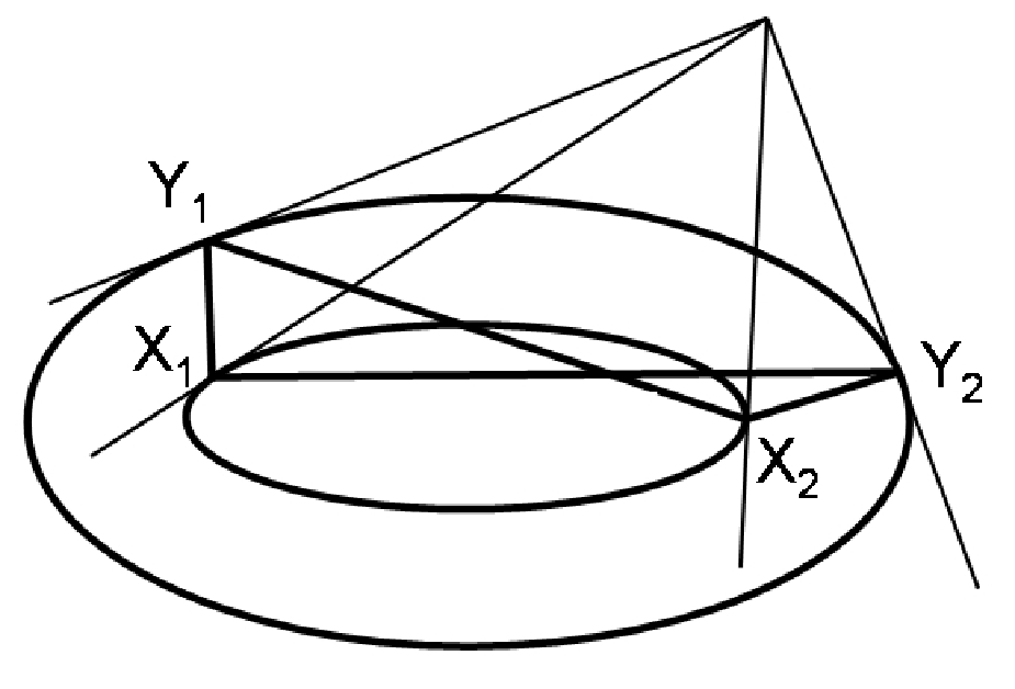
Now, the Darboux’s statement can be generalized and proved as follows:

Theorem 9

Let $\mathcal{Q}_{\lambda_{1}}$ , $\mathcal{Q}_{\lambda_{2}}$ be confocal quadrics, $X_{1}$ , $X_{2}$ points on $\mathcal{Q}_{\lambda_{1}}$ and $Y_{1}$ , $Y_{2}$ on $\mathcal{Q}_{\lambda_{2}}$ . If the tangent hyperplanes at these points to the quadrics belong to a pencil, then $X_{1},X_{2},Y_{1},Y_{2}$ constitute a virtual reflection configuration.

Furthermore, if $\mathcal{Q}_{\lambda_{1}}$ and $\mathcal{Q}_{\lambda_{2}}$ are ellipsoids and $\lambda_{1}>\lambda_{2}$ , then the sides of the quadrilateral $X_{1}Y_{1}X_{2}Y_{2}$ obey the real reflection from $\mathcal{Q}_{\lambda_{2}}$ and the virtual reflection from $\mathcal{Q}_{\lambda_{1}}$ .

Proof. Denote by $\xi_{1}$ , $\xi_{2}$ and $\eta_{1}$ , $\eta_{2}$ the tangent hyperplanes to $\mathcal{Q}_{\lambda_{1}}$ at $X_{1}$ , $X_{2}$ and to $\mathcal{Q}_{\lambda_{2}}$ at $Y_{1}$ , $Y_{2}$ , respectively. All these hyperplanes belong to a pencil, thus their poles with respect to any quadric will be collinear – particularly, the pole $P$ of $\xi_{1}$ lies on line $Y_{1}Y_{2}$ . If $Q=Y_{1}Y_{2}\cap\xi_{1}$ , then pairs $P$ , $Q$ and $Y_{1}$ , $Y_{2}$ are harmonically conjugate. It follows that the lines $X_{1}Y_{1}$ , $X_{1}Y_{2}$ obey the reflection law from $\xi_{1}$ . We prove similarly that all other adjacent sides of the quadrilateral $X_{1}Y_{1}X_{2}Y_{2}$ obey the law of reflection on the corresponding quadrics.

Now, suppose that $\mathcal{Q}_{\lambda_{1}}$ , $\mathcal{Q}_{\lambda_{2}}$ are ellipsoids, and $\lambda_{1}>\lambda_{2}$ . This means that $\mathcal{Q}_{\lambda_{1}}$ is placed inside $\mathcal{Q}_{\lambda_{2}}$ , thus the whole quadrilateral $X_{1}Y_{1}X_{2}Y_{2}$ is inside $\mathcal{Q}_{\lambda_{2}}$ . This means that the reflections in points $Y_{1}$ , $Y_{2}$ are real reflections from inside on $\mathcal{Q}_{\lambda_{2}}$ . Besides, the ellipsoid $\mathcal{Q}_{\lambda_{1}}$ is completely placed inside the dihedron with the sides $\eta_{1}$ , $\eta_{2}$ . This ellipsoid is also inside the dihedron $\angle(\xi_{1},\xi_{2})$ . Since planes $\eta_{1}$ i $\eta_{2}$ are outside $\angle(\xi_{1},\xi_{2})$ , it follows that points $Y_{1}$ , $Y_{2}$ are also outside this dihedron. Thus, points $Y_{1}$ , $Y_{2}$ are placed at the different sides of each of the planes $\xi_{1}$ , $\xi_{2}$ , and reflections of $\mathcal{Q}_{\lambda_{1}}$ are virtual. $\Box$

We are going to conclude this section with the statement converse to the previous theorem.

Proposition 6

Let pairs of points $X_{1}$ , $X_{2}$ and $Y_{1}$ , $Y_{2}$ belong to confocal ellipsoids $\mathcal{Q}_{1}$ and $\mathcal{Q}_{2}$ , and let $\alpha_{1}$ , $\alpha_{2}$ , $\beta_{1}$ , $\beta_{2}$ be the corresponding tangent planes. If a quadruple $X_{1},X_{2},Y_{1},Y_{2}$ is a virtual reflection configuration, then planes $\alpha_{1}$ , $\alpha_{2}$ , $\beta_{1}$ , $\beta_{2}$ belong to a pencil.

Proof. Consider the pencil determined by $\alpha_{1}$ and $\beta_{1}$ . Let $\alpha_{2}^{\prime}$ , $\beta_{2}^{\prime}$ be planes of this pencil, tangent respectively to $\mathcal{Q}_{1}$ , $\mathcal{Q}_{2}$ at points $X_{2}^{\prime}$ , $Y_{2}^{\prime}$ , and distinct from $\alpha_{1}$ and $\beta_{1}$ . By Theorem 9, the quadruple $X_{1},X_{2}^{\prime},Y_{1},Y_{2}^{\prime}$ is a virtual reflection configuration. Moreover, if denote by $\lambda_{1}$ , $\lambda_{2}$ parameters of $\mathcal{Q}_{1}$ , $\mathcal{Q}_{2}$ and assume $\lambda_{1}>\lambda_{2}$ , then the sides of the quadrangle obey the reflection law at points $Y_{1},Y_{2}^{\prime}$ and the virtual reflection at $X_{1},X_{2}^{\prime}$ . Since the ray obtained from $X_{1}Y_{1}$ by the virtual reflection of $\mathcal{Q}_{1}$ at $X_{1}$ , has only one intersection with $\mathcal{Q}_{2}$ , we have $Y_{2}=Y_{2}^{\prime}$ . Points $X_{2}$ and $X_{2}^{\prime}$ coincide, being the intersection of rays obtained from $Y_{1}X_{1}$ and $Y_{2}X_{1}$ , by the reflection at the quadric $\mathcal{Q}_{2}$ . Now, the four tangent planes are all in one pencil. $\Box$

8 On Generalization of Lebesgue’s Proof of Cayley’s Condition

In this section, the analysis of possibility of generalization of the inspiring Lebesgue’s procedure to higher dimensional cases will be given.

A higher dimensional analogue of the crucial lemma from [31], which is Lemma 1 of this article, is the following:

Lemma 9

Let $\mathcal{Q}_{1}$ , $\mathcal{Q}_{2}$ be quadrics of a confocal system and let lines $\ell_{1}$ , $\ell_{2}$ satisfy the reflection law at point $X_{1}$ of $\mathcal{Q}_{1}$ and $\ell_{2}$ , $\ell_{3}$ at $Y_{2}$ of $\mathcal{Q}_{2}$ . Then line $\ell_{1}$ meets $\mathcal{Q}_{2}$ at point $Y_{1}$ and $\ell_{3}$ meets $\mathcal{Q}_{1}$ at point $X_{2}$ such that pairs of lines $\ell_{1}$ , $Y_{1}X_{2}$ and $Y_{1}X_{2}$ , $\ell_{3}$ satisfy the reflection law at points $Y_{1}$ , $X_{2}$ of quadrics $\mathcal{Q}_{2}$ , $\mathcal{Q}_{1}$ respectively. Moreover, tangent planes at $X_{1}$ , $X_{2}$ , $Y_{1}$ , $Y_{2}$ of these two quadrics are in the same pencil.

This statement can be proved by the direct application of Theorem 9 on virtual reflections. Nevertheless, there is no complete analogy between Lemma 9 and the corresponding assertion in plane. Lines $\ell_{1}$ , $\ell_{3}$ and $\ell_{2}$ , $Y_{1}Y_{2}$ are generically skew. Hence we do not have the third pair of planes tangent to the quadric, containing intersection points of these two pairs of lines.

Nevertheless, a complete generalization of the Basic Lemma, can be formulated as follows:

Theorem 10

Let $\mathcal{F}$ be a dual pencil of quadrics in the three-dimensional space.

For a given quadric $\Gamma_{0}\in\mathcal{F}$ , there exist quadruples $\alpha$ , $\beta$ , $\gamma$ , $\delta$ of planes tangent to $\Gamma_{0}$ , and quadrics $\Gamma_{1},\Gamma_{2},\Gamma_{3}\in\mathcal{F}$ touching the pairs of intersecting lines $\alpha\beta$ and $\gamma\delta$ , $\alpha\gamma$ and $\beta\delta$ , $\alpha\delta$ and $\beta\gamma$ respectively, with the tangent planes to $\Gamma_{1}$ , $\Gamma_{2}$ , $\Gamma_{3}$ at points of tangency with the lines, all being in one pencil $\Delta$ . Moreover, the six intersecting lines are in one bundle.

Every such a configuration of planes $\alpha$ , $\beta$ , $\gamma$ , $\delta$ and quadrics $\Gamma_{0}$ , $\Gamma_{1}$ , $\Gamma_{2}$ , $\Gamma_{3}$ is determined by two of the intersecting lines, and the tangent planes to $\Gamma_{1}$ , $\Gamma_{2}$ , or $\Gamma_{3}$ corresponding to these two lines.

Proof. Suppose first that two adjacent lines $\alpha\beta$ and $\alpha\gamma$ are given. There exist two quadrics in $\mathcal{F}$ touching $\alpha\beta$ — let $\Gamma_{1}$ be the one tangent to the given plane $\mu\supset\alpha\beta$ . $\Gamma_{2}$ denotes the quadric that touches $\alpha\gamma$ and the given plane $\pi\supset\alpha\gamma$ . The pencil $\Delta$ is determined by its planes $\mu$ and $\pi$ . All three lines $\alpha\beta$ , $\alpha\gamma$ , $\Delta$ are in one bundle $\mathcal{B}$ , see Figure 11.

Note that lines $\alpha\beta$ and $\alpha\gamma$ determine plane $\alpha$ and that $\alpha$ touches a unique quadric $\Gamma_{0}$ from $\mathcal{F}$ . Thus, $\beta$ and $\gamma$ are determined as tangent planes to $\Gamma_{0}$ , containing lines $\alpha\beta$ and $\alpha\gamma$ respectively and being different from $\alpha$ .

Let $\nu$ be the plane from $\Delta$ , other than $\mu$ , that is touching $\Gamma_{1}$ . We are going to prove that the point of tangency $\nu$ with $\Gamma_{1}$ belongs to $\gamma$ .

Denote by $\Phi$ the dual pencil determined by quadric $\Gamma_{1}$ and the degenerate quadric which consists of lines $\alpha\beta$ and $\gamma\nu$ . Since $\gamma\nu\in\mathcal{B}$ , these two lines are coplanar.

Dual pencils $\mathcal{F}$ and $\Phi$ determine the same involution of the pencil $\alpha\gamma$ , because they both determine the pair $\alpha,\gamma$ and the quadric $\Gamma_{1}$ is the common for both pencils. Since quadric $\Gamma_{2}\in\mathcal{F}$ determines the pair $\pi,\pi$ of coinciding planes, a quadric $\mathcal{Q}$ determining the same pair has to exist in $\Phi$ . This quadric, as well as all other quadrics in $\Phi$ , touches $\nu$ and $\mu$ . Since $\nu$ , $\mu$ , $\pi$ all belong to the pencil $\Delta$ , $\mathcal{Q}$ is degenerate and contains $\Delta$ . Since any quadric of $\Phi$ touches $\mu$ , $\pi$ at points of lines $\alpha\beta$ , $\alpha\gamma$ respectively, the other component of $\mathcal{Q}$ also has to be $\Delta$ , thus $\mathcal{Q}$ is the double $\Delta$ .

It follows that all quadrics of $\Phi$ , and particularly $\Gamma_{1}$ , are tangent to $\nu$ at a point of $\gamma\nu$ .

Similarly, if $\kappa\neq\pi$ is the other plane in $\Delta$ tangent to $\Gamma_{2}$ , the touching point belongs to $\beta$ and to $\delta$ , the plane, other than $\gamma$ , tangent to $\Gamma_{0}$ and containing the line $\gamma\nu$ .

Now, let us note that $\mathcal{F}$ and $\Phi$ determine the same involution on pencil $\alpha\delta$ , because they both determine pair $\alpha,\delta$ and $\Gamma_{1}$ belongs to both pencils. Thus, the common plane $\rho$ of pencils $\Delta$ and $\alpha\delta$ is tangent to a quadric of $\mathcal{F}$ at a point of $\alpha\delta$ . Denote this quadric by $\Gamma_{3}$ . Similarly as before, we can prove that $\Gamma_{3}$ is touching the line $\beta\gamma$ and the corresponding tangent plane $\sigma$ is common to pencils $\Delta$ and $\beta\gamma$ .

Now, suppose that two non-adjacent lines $\alpha\beta$ , $\gamma\delta$ , both tangent to a quadric $\Gamma_{1}\in\mathcal{F}$ , with the corresponding tangent planes $\mu$ , $\nu$ , are given. Similarly as above, we can prove that the plane $\rho$ is tangent to a quadric from $\mathcal{F}$ at a point of $\alpha\delta$ . So, we can consider the configuration as determined by adjacent lines $\alpha\beta$ , $\alpha\delta$ and planes $\mu$ , $\rho$ . In this way, we reduced it to the previous case. $\Box$

For the conclusion, we will generalize the notion of Cayley’s cubic.

Definition 4

The generalized Cayley curve is the variety of hyperplanes tangent to quadrics of a given confocal family in $\mathbb{C}P^{d}$ at the points of a given line $\ell$ .

This curve is naturally embedded in the dual space $\mathbb{C}P^{d\,*}$ .

On Figure 12, we see the planes which correspond to one point of the line $\ell$ in the 3-dimensional space.

Proposition 7

The generalized Cayley curve in $\mathbb{C}^{d}$ , for $d\geq 3$ is a hyperelliptic curve of genus $g=d-1$ . Its natural realization in $\mathbb{C}^{d\,*}$ is of degree $2d-1$ .

Proof. Let us consider the projection from the generalized Cayley’s curve to the line of the parameters of the confocal family. Since $\ell$ intersects each quadric twice, this is a two-folded covering, with branching points corresponding to quadrics touching $\ell$ and the degenerate ones. Since there is $(d-1)+(d+1)$ such quadrics, we obtain the genus directly from Riemann-Hurwitz formula.

Its degree is equal to the number of intersection points with a hyperplane in $\mathbb{C}^{d\,*}$ . Such a hyperplane is a bundle of hyperplanes containing one point in $\mathbb{C}^{d}$ . Take $P\in\ell$ to be this point. Since there are $d$ quadrics from the confocal family containing $P$ and $d-1$ tangent to $\ell$ , the assertion follows. $\Box$

Let us note that this curve is isomorphic to the Veselov-Moser isospectral curve (7). Also, in the 3-dimensional case, it is isomorphic to the Jacobi hyperelliptic curve, which was used by Darboux considering the generalization of Poncelet theorem.

Further development of these ideas will be presented in the separate publication [22].

Appendix 1
Integrable Potential Perturbations of the Elliptical Billiard

The equation

\lambda V_{xy}+3\left(yV_{x}-xV_{y}\right)+(y^{2}-x^{2})V_{xy}+xy\left(V_{xx}-V_{yy}\right)=0,

(10)

is a special case of the Bertrand-Darboux equation [8, 14, 36], which represents the necessary and sufficient condition for a natural mechanical system with two degrees of freedom

H=\frac{1}{2}(p^{2}_{x}+p^{2}_{y})+V(x,y)

to be separable in elliptical coordinates or some of their degenerations.

Solutions of Equation (10) in the form of Laurent polynomials in $x,y$ were described in [16]. Such solutions are in [18] naturally related to the well-known hypergeometric functions of Appell. This relation automatically gives a wider class of solutions of Equation (10) – new potentials are obtained for non-integer parameters, giving a huge family of integrable billiards within an ellipse with potentials. Similar formulae for potential perturbations for the Jacobi problem for geodesics on an ellipsoid from [16, 17] are given. They show the existence of a connection between separability of classical systems on one hand, and the theory of hypergeometric functions on the other one, which is still not completely understood. Basic references for the Appell functions are [2, 3, 35].

The function $F_{4}$ is one of the four hypergeometric functions in two variables, which are introduced by Appell [2, 3]:

F_{4}(a,b,c,d;x,y)=\sum\frac{(a)_{m+n}(b)_{m+n}}{(c)_{m}(d)_{n}}\frac{x^{m}}{m!}\frac{y^{n}}{n!},

where $(a)_{n}$ is the standard Pochhammer symbol:

	$\displaystyle(a)_{n}$	$\displaystyle=\frac{\Gamma(a+n)}{\Gamma(a)}=a(a+1)\dots(a+n-1),$
	$\displaystyle(a)_{0}$	$\displaystyle=1.$

(For example $m!=(1)_{m}.$ )

The series is convergent for $\sqrt{x}+\sqrt{y}\leq 1$ . The functions $F_{4}$ can be analytically continued to the solutions of the equations:

	$\displaystyle x(1-x)\frac{\partial^{2}F}{\partial x^{2}}$	$\displaystyle-y^{2}\frac{\partial^{2}F}{\partial y^{2}}-2xy\frac{\partial^{2}F}{\partial x\partial y}+$
		$\displaystyle+[c-(a+b+1)x]\frac{\partial F}{\partial x}-(a+b+1)y\frac{\partial F}{\partial y}-abF=0,$
	$\displaystyle y(1-y)\frac{\partial^{2}F}{\partial y^{2}}$	$\displaystyle-x^{2}\frac{\partial^{2}F}{\partial x^{2}}-2xy\frac{\partial^{2}F}{\partial x\partial y}+$
		$\displaystyle+[c^{\prime}-(a+b+1)y]\frac{\partial F}{\partial y}-(a+b+1)x\frac{\partial F}{\partial x}-abF=0,$

A1.1 Potential Perturbations of a Billiard inside an Ellipse

A billiard system which describes a particle moving freely within the ellipse

\frac{x^{2}}{A}+\frac{y^{2}}{B}=1

is completely integrable and it has an additional integral

K_{1}=\frac{\dot{x}^{2}}{A}+\frac{\dot{y}^{2}}{B}-\frac{(\dot{x}y-\dot{y}x)^{2}}{AB}.

We are interested now in potential perturbations $V=V(x,y)$ such that the perturbed system has an integral $\tilde{K}_{1}$ of the form

\tilde{K}_{1}=K_{1}+k_{1}(x,y),

where $k_{1}=k_{1}(x,y)$ depends only on coordinates. This specific condition leads to Equation (10) on $V$ with $\lambda=A-B$ .

In [16, 17] the Laurent polynomial solutions of Equation (10) were given. Denoting

V_{\gamma}=\tilde{y}^{-\gamma}\bigl((1-\gamma)\,\tilde{x}\,F_{4}(1,2-\gamma,2,1-\gamma,\tilde{x},\tilde{y})+1\bigr),

(11)

where $\tilde{x}=x^{2}/\lambda$ , $\tilde{y}=-y^{2}/\lambda$ , the more general result was obtained in [18]:

Theorem 11

Every function $V_{\gamma}$ given with (11) and $\gamma\in\mathbb{C}$ is a solution of Equation (10).

This theorem gives new potentials for non-integer $\gamma$ . For integer $\gamma$ , one obtains the Laurent solutions.

Mechanical Interpretation. With $\gamma\in\mathbb{R}^{-}$ and the coefficient multiplying $V_{\gamma}$ positive, we have a potential barrier along $x$ -axis. We can consider billiard motion in the upper half-plane. Then we can assume that a cut is done along negative part of $y$ -axis, in order to get a unique-valued real function as a potential.

Solutions of Equation (10) are also connected with interesting geometric subjects.

A1.2 The Jacobi Problem for Geodesics on an Ellipsoid

The Jacobi problem for the geodesics on an ellipsoid

\frac{x^{2}}{A}+\frac{y^{2}}{B}+\frac{z^{2}}{C}=1

has an additional integral

K_{1}=\left(\frac{x^{2}}{A^{2}}+\frac{y^{2}}{B^{2}}+\frac{z^{2}}{C^{2}}\right)\left(\frac{\dot{x}^{2}}{A}+\frac{\dot{y}^{2}}{B}+\frac{\dot{z}^{2}}{C}\right).

Potential perturbations $V=V(x,y,z)$ , such that perturbed systems have integrals of the form

\tilde{K}_{1}=K_{1}+k(x,y,z),

satisfy the following system:

$\displaystyle\left(\frac{x^{2}}{A^{2}}+\frac{y^{2}}{B^{2}}+\frac{z^{2}}{C^{2}}\right)$	$\displaystyle V_{xy}\frac{A-B}{AB}-3\frac{y}{B^{2}}\frac{V_{x}}{A}+3\frac{x}{A^{2}}\frac{V_{y}}{B}+$	(12)
$\displaystyle+\left(\frac{x^{2}}{A^{3}}-\frac{y^{2}}{B^{3}}\right)$	$\displaystyle V_{xy}+\frac{xy}{AB}\left(\frac{V_{yy}}{A}-\frac{V_{xx}}{B}\right)+\frac{zx}{CA^{2}}V_{zy}-\frac{zy}{CB^{2}}V_{zx}=0$

$\displaystyle\left(\frac{x^{2}}{A^{2}}+\frac{y^{2}}{B^{2}}+\frac{z^{2}}{C^{2}}\right)$	$\displaystyle V_{yz}\frac{B-C}{BC}-3\frac{z}{C^{2}}\frac{V_{y}}{B}+3\frac{y}{B^{2}}\frac{V_{z}}{C}+$
$\displaystyle+\left(\frac{y^{2}}{B^{3}}-\frac{z^{2}}{C^{3}}\right)$	$\displaystyle V_{yz}+\frac{yz}{BC}\left(\frac{V_{zz}}{B}-\frac{V_{yy}}{C}\right)+\frac{xy}{AB^{2}}V_{xz}-\frac{xz}{AC^{2}}V_{xy}=0$

$\displaystyle\left(\frac{x^{2}}{A^{2}}+\frac{y^{2}}{B^{2}}+\frac{z^{2}}{C^{2}}\right)$	$\displaystyle V_{zx}\frac{C-A}{AC}-3\frac{x}{A^{2}}\frac{V_{z}}{C}+3\frac{z}{C^{2}}\frac{V_{x}}{A}+$
$\displaystyle+\left(\frac{z^{2}}{C^{3}}-\frac{x^{2}}{A^{3}}\right)$	$\displaystyle V_{zx}+\frac{xz}{AC}\left(\frac{V_{xx}}{C}-\frac{V_{zz}}{A}\right)+\frac{zy}{BC^{2}}V_{xy}-\frac{yx}{BA^{2}}V_{yz}=0.$

This system is an analogue of the Bertrand-Darboux equation (10) (see [18]).

Let

\frac{x^{2}C(A-C)}{z^{2}(B-A)A}=\hat{x},\quad\frac{y^{2}C(C-B)}{z^{2}(B-A)B}=\hat{y}.

The following statement was also proved in [18]:

Theorem 12

For every $\gamma\in\mathbb{C}$ , the function

V_{\gamma}=(-\gamma+1)\left(\frac{z^{2}}{x^{2}}\right)^{\gamma}F_{4}(1,-\gamma+2,2,-\gamma+1,\hat{x},\hat{y})

is a solution of the system (12).

Thus, by solving Bertrand–Darboux equation and its generalizations, as it is done in Theorems 11 and 12, one get large families of separable mechanical systems with two degrees of freedom. It is well known that separable systems of two degrees of freedom are necessarily of the Liouville type, see [36].

Now the natural question of Poncelet type theorem describing periodic solutions of such perturbed billiard systems arises. It appears that again Darboux studied such a question, since in [15], he analyzed generalizations of Poncelet theorem in the case of the Liouville surfaces.

Appendix 2
Poncelet Theorem on Liouville Surfaces

In this section, we are going to give the presentation and comments to the Darboux results on the generalization of Poncelet theorem to Liouville surfaces.

A2.1 Liouville Surfaces and Families of Geodesic Conics

In this subsection, following [15], we are going to define geodesic conics on an arbitrary surface, derive some important properties of theirs and finally to obtain an important characterization of Liouville surfaces via families of geodesic conics.

Let $\mathcal{C}_{1}$ and $\mathcal{C}_{2}$ be two fixed curves on a given surface $\mathcal{S}$ . Geodesic ellipses and hyperbolae on $\mathcal{S}$ are curves given by the equations:

\hfil\displaystyle\theta+\sigma=\mathrm{const},

\hfil\displaystyle\theta-\sigma=\mathrm{const},

where $\theta$ , $\sigma$ are geodesic distances from $\mathcal{C}_{1}$ , $\mathcal{C}_{2}$ respectively.

A coordinate system composed of geodesic ellipses and hyperbolae joined to two fixed curves is orthogonal. In the following proposition, we are going to describe all orthogonal coordinate systems with coordinate curves that can be regarded as a family of geodesic ellipses and hyperbolae.

Proposition 8

Let

ds^{2}=A^{2}du^{2}+C^{2}dv^{2}

(13)

be the surface element corresponding to an orthogonal system of coordinate curves. Then the coordinate curves represent a family of geodesic ellipses and hyperbolae if and only if the coefficients $A$ , $C$ satisfy a relation of the form:

\frac{U}{A^{2}}+\frac{V}{C^{2}}=1,

with $U$ and $V$ being functions of $u$ , $v$ respectively.

Proof. By assumption, equations of coordinate curves are:

\theta+\sigma=\mathrm{const},\quad\theta-\sigma=\mathrm{const},

with $\theta$ , $\sigma$ representing geodesic distances from a point of the surface to two fixed curves.

Thus:

u=F(\theta+\sigma),\qquad v=F_{1}(\theta-\sigma).

Solving these equations with respect to $\theta$ and $\sigma$ , we obtain:

\theta=\phi(u)+\psi(v),\quad\sigma=\phi(u)-\psi(v).

As geodesic distances, $\theta$ and $\sigma$ need to satisfy the characteristic partial differential equation:

\frac{A^{2}(\frac{\partial\xi}{\partial v})^{2}+C^{2}(\frac{\partial\xi}{\partial u})^{2}}{A^{2}C^{2}}=1.

(14)

From there, we deduce the desired relation with $U=(\phi^{\prime}(u))^{2}$ , $V=(\psi^{\prime}(v))^{2}$ .

The converse is proved in a similar manner. $\Box$

As a straightforward consequence, the following interesting property is obtained:

Corollary 3

If an orthogonal system of curves can be regarded as a system of geodesic ellipses and hyperbolae in two different ways, then it can be regarded as such a system in infinitely many ways.

Now, let us concentrate to Liouville surfaces, i.e. to surfaces with the surface element of the form

ds^{2}=(U-V)(U_{1}^{2}du^{2}+V_{1}^{2}dv^{2}),

(15)

where $U$ , $U_{1}$ and $V$ , $V_{1}$ depend only on $u$ and $v$ respectively.

Now, we are ready to present the characterization of Liouville surfaces via geodesic conics.

Theorem 13

An orthogonal system on a surface can be regarded in two different manners as a system of geodesic conics if and only if it is of the Liouville form.

Proof. Consider a surface with the element (13). If coordinate lines $u=\mathrm{const}$ , $v=\mathrm{const}$ can be regarded as geodesic conics in two different manners then, by Proposition 6, $A$ , $C$ satisfy two different equations:

\frac{U}{A^{2}}+\frac{V}{C^{2}}=1,\qquad\frac{U_{1}}{A^{2}}+\frac{V_{1}}{C^{2}}=1.

Solving them with respect to $A$ , $C$ , we obtain that the surface element is of the form

ds^{2}=\left(\frac{U}{U-U_{1}}+\frac{V}{V_{1}-V}\right)\bigl((U-U_{1})du^{2}+(V_{1}-V)dv^{2}\bigr).

Conversely, consider the Liouville surface with the element (15) and the following solutions of the equation (14):

\hfil\displaystyle\theta=\int U_{1}\sqrt{U-a}\,du+\int V_{1}\sqrt{a-V}dv,

\hfil\displaystyle\sigma=\int U_{1}\sqrt{U-a}\,du-\int V_{1}\sqrt{a-V}dv.

The equations $\theta+\sigma=\mathrm{const}$ , $\theta-\sigma=\mathrm{const}$ will define the coordinate curves. $\Box$

A2.2 Generalization of Graves and Poncelet Theorems to Liouville Surfaces

We learned from Darboux [15] that Liouville surfaces are exactly these having an orthogonal system of curves that can be regarded in two or, equivalently, infinitely many different ways, as geodesic conics. Now, we are going to present how to make a choice, among these infinitely many presentations, of the most convenient one, which will enable us to show the generalizations of theorems of Graves and Poncelet. All these ideas of enlightening beauty and profoundness belong to Darboux [15].

Consider a curve $\gamma$ on a surface $\mathcal{S}$ . The involute of $\gamma$ with respect to a point $A\in\gamma$ is the set of endpoints $M$ of all geodesic segments $TM$ , such that:

$T\in\gamma$ ;

$TM$ is tangent to $\gamma$ at $T$ ;

the length of $TM$ is equal to the length of the segment $TA\subset\gamma$ ; and

these two segments are placed at the same side of the point $T$ .

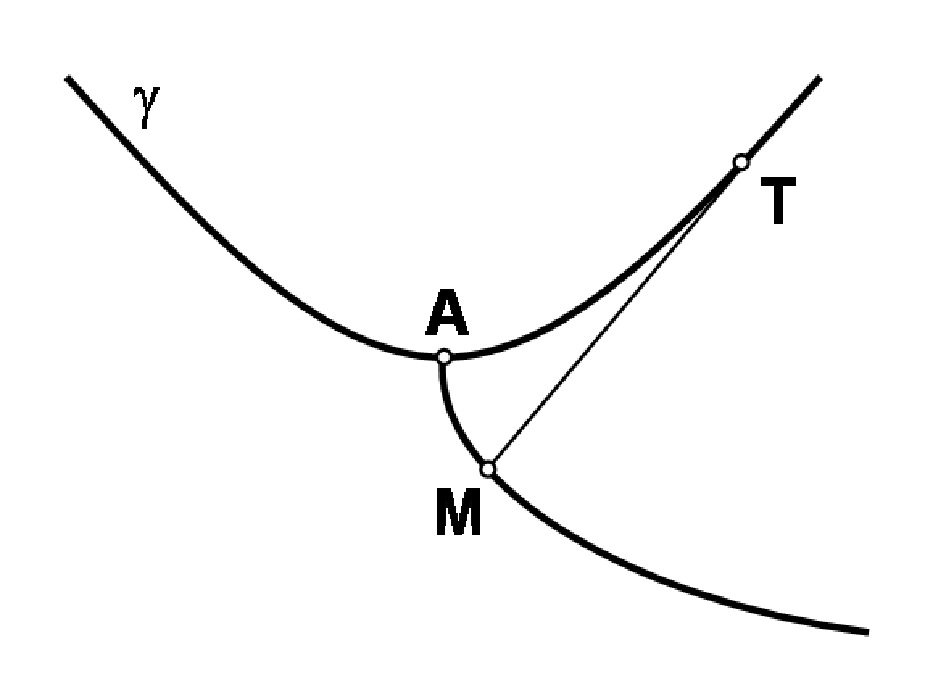
Involutes have the following important property, which follows immediately from the definition:

Lemma 10

The geodesic segments $TM$ are orthogonal to the involute, and the involute itself is orthogonal to $\gamma$ at $A$ .

Now, we are going to find explicitly the equations of involutes of coordinate curves on a Liouville surface $\mathcal{S}$ with the surface element (15).

Lemma 11

The curves on $\mathcal{S}$ given by the equations:

	$\displaystyle\theta$	$\displaystyle=\int U_{1}\sqrt{U-a}\,du+\int V_{1}\sqrt{a-V}dv=\mathrm{const},$		(16)
	$\displaystyle\sigma$	$\displaystyle=\int U_{1}\sqrt{U-a}\,du-\int V_{1}\sqrt{a-V}dv=\mathrm{const}$		(16)

are involutes of the coordinate curve whose parameter satisfies the equation:

(U-a)(V-a)=0.

Proof. Fix the parameter $a$ . The equations of of geodesics normal to the curves $\theta=\mathrm{const}$ , $\sigma=\mathrm{const}$ are obtained by differentiating (16) with respect to $a$ :

\frac{U_{1}du}{\sqrt{U-a}}\pm\frac{V_{1}dv}{\sqrt{a-V}}=0.

(17)

Let $u_{0}$ be a solution of the equation $U-a=0$ . Then, the geodesic line (17) will satisfy $du=0$ at the point of intersection with the curve $u=u_{0}$ , i.e. it will be tangent to this coordinate curve. The statement now follows from Lemma 10. $\Box$

Proposition 9

Coordinate curves on a Liouville surface are geodesic conics with respect to any two involutes of one of them.

Proof. Follows from Lemma 11 and the proof of Theorem 13. $\Box$

Now, we are ready to prove the generalization of Graves’ theorem.

Theorem 14

Let $\mathcal{E}_{0}:u=u_{0}$ and $\mathcal{E}_{1}:u=u_{1}$ be coordinate curves on the Liouville surface $\mathcal{S}$ . For a point $M\in\mathcal{E}_{1}$ , denote by $MP$ and $MP^{\prime}$ geodesic segments that touch $\mathcal{E}_{0}$ at $Q$ , $Q^{\prime}$ . Then the expression

\ell(MP)+\ell(MP^{\prime})-\ell(PP^{\prime})

is constant for all $M$ , where $\ell(MP)$ , $\ell(MP^{\prime})$ , and $\ell(PP^{\prime})$ denote lengths of geodesic segments $MP$ , $MP^{\prime}$ , and of the segment $PP^{\prime}\subset\mathcal{E}_{0}$ respectively.

Proof. Let $\mathcal{D}$ , $\mathcal{D}^{\prime}$ be involutes of the curve $\mathcal{E}_{0}$ with respect to points $R,R^{\prime}\in\mathcal{E}_{0}$ , and $Q,Q^{\prime}$ intersections of geodesics $MP,MP^{\prime}$ with these involutes.

Both $\mathcal{E}_{0}$ and $\mathcal{E}_{1}$ are geodesic ellipses with base curves $\mathcal{D}$ , $\mathcal{D}^{\prime}$ , thus the sum $\ell(MQ)+\ell(MQ^{\prime})$ remains constant when $M$ moves on $\mathcal{E}_{1}$ .

Since $\ell(PR)=\ell(MP)+\ell(MQ)$ , $\ell(P^{\prime}R^{\prime})=\ell(MP^{\prime})+\ell(MQ^{\prime})$ , we have:

	$\displaystyle\ell(MQ)+\ell(MQ^{\prime})$	$\displaystyle=\ell(PR)+\ell(P^{\prime}R^{\prime})-\ell(MP)-\ell(MP^{\prime})$
		$\displaystyle=\ell(RR^{\prime})-\bigl(\ell(MP)+\ell(MP^{\prime})-\ell(PP^{\prime})\bigr),$

and the theorem is proved. $\Box$

From here, the complete analogue of the Poncelet theorem can be derived:

Theorem 15

Let us consider a polygon on the Liouville surface $\mathcal{S}$ , with all sides being geodesics tangent to a given coordinate curve, and each vertex but one moving on a coordinate curve. Then the last vertex also remains on a fixed coordinate curve.

Acknowledgements

The research was partially supported by the Serbian Ministry of Science and Technology, Project Geometry and Topology of Manifolds and Integrable Dynamical Systems. The authors would like to thank Prof. B. Dubrovin, Yu. Fedorov and S. Abenda for interesting discussions, and to Prof. M. Berger for historical remarks. One of the authors (M.R.) acknowledges her gratitude to Prof. V. Rom-Kedar and the Weizmann Institute of Science for the kind hospitality and support during in the final stage of the work on this paper.

References

[1] S. Abenda, Yu. Fedorov, Closed geodesics and billiards on quadrics related to elliptic KdV solutions, preprint, arXiv nlin.SI/0412034, 2004.
[2] P. Appell, Sur les fonctions hypergéométriques de deux variables et sur des équations lineaires aux derivées partielles, Comptes Rendus 90 (1880), p. 296.
[3] P. Appell, J. Kempe de Feriet, Fonctions hypergéométriques et hyperspheriques, in Polynomes d’Hermite, Gauthier Villars, Paris, 1926.
[4] V. Arnol’d, Mathematical Methods of Classical Mechanics, Springer-Verlag, New York, 1978.
[5] W. Barth, Th. Bauer, Poncelet theorems, Expo. Math. 14 (1996), 125-144.
[6] W. Barth, J. Michel, Modular curves and Poncelet polygons, Math. Ann. 295 (1993), 25-49.
[7] M. Berger, Geometry, Springer-Verlag, Berlin, 1987.
[8] J. Bertrand, Jour. de Math. 17 (1852), p. 121.
[9] H. J. M. Bos, C. Kers, F. Oort, D. W. Raven, Poncelet’s closure theorem, Expo. Math. 5 (1987), 289-364.
[10] A. Cayley, Developments on the porism of the in-and-circumscribed polygon, Philosophical magazine 7 (1854), 339-345.
[11] S.-J. Chang, B. Crespi B, K.-J. Shi, Elliptical billiard systems and the full Poncelet’s theorem in $n$ dimensions, J. Math. Phys. 34 (1993), no. 6, 2242-2256.
[12] S.-J. Chang, K. J. Shi, Billiard systems on quadric surfaces and the Poncelet theorem, J. Math. Phys. 30 (1989), no. 4, 798-804.
[13] G. Darboux, Sur les polygones inscrits et circonscrits à l’ellipsoïde, Bulletin de la Société philomathique 7 (1870), 92-94.
[14] G. Darboux, Archives Neerlandaises (2) 6 (1901), p. 371.
[15] G. Darboux, Leçons sur la théorie générale des surfaces et les applications géométriques du calcul infinitesimal, volumes 2 and 3, Gauthier-Villars, Paris, 1914.
[16] V. Dragović, On integrable potential perturbations of the Jacobi problem for the geodesics on the ellipsoid, J. Phys. A: Math. Gen. 29 (1996), no. 13, L317-L321.
[17] V. I. Dragovich, Integrable perturbations of the Birkgof billiard inside an ellipse (in Russian), Prikladnaya matematika i mehanika, 62 (1998), no. 1, 166-169.
[18] V. Dragović, The Appell hypergeometric functions and classical separable mechanical systems, J. Phys A: Math. Gen. 35 (2002), no. 9, 2213-2221.
[19] V. Dragović, M. Radnović, Conditions of Cayley’s type for ellipsoidal billiard, J. Math. Phys. 39 (1998), no. 1, 355-362.
[20] V. Dragović, M. Radnović, On periodical trajectories of the billiard systems within an ellipsoid in $\mathbb{R}^{d}$ and generalized Cayley’s condition, J. Math. Phys. 39 (1998), no. 11, 5866-5869.
[21] V. Dragović, M. Radnović, Cayley-type conditions for billiards within $k$ quadrics in $\mathbb{R}^{d}$ , J. of Phys. A: Math. Gen. 37 (2004), 1269-1276.
V. Dragović, M. Radnović, Corrigendum: Cayley-type conditions for billiards within $k$ quadrics in $\mathbb{R}^{d}$ , J. of Phys. A: Math. Gen. 38 (2005), 7927.
arXiv: math-ph/0503053
[22] V. Dragović, M. Radnović, Algebra of pencils of quadrics, billiards and closed geodesics, to appear.
[23] P. Griffiths, J. Harris, A Poncelet theorem in space, Comment. Math. Helvetici, 52 (1977), no. 2, 145-160.
[24] P. Griffiths, J. Harris, On Cayley’s explicit solution to Poncelet’s porism, Enseign. Math. 24 (1978), no. 1-2, 31-40.
[25] R. C. Gunning, Lectures on Riemann Surfaces, Princeton University Press, Princeton, NJ, 1966.
[26] C. Hermite, Œuvres de Charles Hermite, vol. III, Gauthier-Villars, Paris, 1912.
[27] C. Jacobi, Vorlesungen über Dynamic. Gesammelte Werke, Supplementband, Berlin, 1884.
[28] B. Jakob, Moduli of Poncelet polygons, J. reine angew. Math. 436 (1993), 33-44.
[29] H. Knörrer, Geodesics on the ellipsoid, Inventiones math. 59 (1980), 119-143.
[30] V. V. Kozlov, D. V. Treshchëv, Billiards, Amer. Math. Soc., Providence RI, 1991.
[31] H. Lebesgue, Les coniques, Gauthier-Villars, Paris, 1942.
[32] J. Moser, A. P. Veselov, Discrete versions of some classical integrable systems and factorization of matrix polynomials, Comm. Math. Phys. 139 (1991), no. 2, 217-243.
[33] J. Moser, Geometry of quadrics and spectral theory, The Chern Symposium, Springer, New York-Berlin, 1980, pp. 147-188.
[34] J. V. Poncelet, Traité des propriétés projectives des figures, Mett-Paris, 1822.
[35] N. Ja. Vilenkin, A. U. Klimyk, Representations of Lie groups and special functions, Recent Advances, Kluwer Academic Publishers, Dordrecht, 1995 (see in particular p. 208).
[36] E. T. Whittaker, A treatise on the analytical dynamics of particles and rigid bodies, third edition, The University Press, Cambridge, 1927.

Geometry of Integrable Billiards and Pencils of Quadrics

Abstract

1 Introduction

2 Planar Case: d=2d=2, kk – Arbitrary

2.1 Full Poncelet Theorem

Lemma 1

Theorem 1

2.2 Cayley’s Condition

Proposition 1

Proposition 2

2.3 Some Applications of Lebesgue’s Results

Corollary 1

Example 1

3 Points of Finite Order on the Jacobian of a Hyperelliptic Curve

Lemma 2

Lemma 3

Lemma 4

Lemma 5

4 Periodic Billiard Trajectories inside kk Confocal Quadrics in 𝐑𝐝\mathbf{R}^{\mathbf{d}}

Lemma 6

4.1 Billiard inside a Domain Bounded by Confocal Quadrics

Theorem 2

Example 2

4.2 Billiard Ordered Game

Definition 1

Definition 2

Example 3

Theorem 3

Proposition 3

Example 4

Example 5

5 Elliptical Billiard as a Discrete Time System: dd – Arbitrary, k=1k=1

5.1 XYZ Model and Isospectral Curves

Theorem 4

5.2 Characterization of Periodical Billiard Trajectories

Lemma 7

Lemma 8

Theorem 5

Theorem 6

Proposition 4

Example 6

6 Periodic Trajectories of Billiards on Quadrics in 𝐑𝐝\mathbf{R}^{\mathbf{d}}

Theorem 7

Theorem 8

Example 7

Example 8

Example 9

Proposition 5

Corollary 2

7 Virtual Billiard Trajectories

Definition 3

Theorem 9

Proposition 6

8 On Generalization of Lebesgue’s Proof of Cayley’s Condition

Lemma 9

Theorem 10

Definition 4

Proposition 7

Appendix 1 Integrable Potential Perturbations of the Elliptical Billiard

A1.1 Potential Perturbations of a Billiard inside an Ellipse

Theorem 11

A1.2 The Jacobi Problem for Geodesics on an Ellipsoid

Theorem 12

Appendix 2 Poncelet Theorem on Liouville Surfaces

A2.1 Liouville Surfaces and Families of Geodesic Conics

Proposition 8

Corollary 3

Theorem 13

A2.2 Generalization of Graves and Poncelet Theorems to Liouville Surfaces

Lemma 10

Lemma 11

Proposition 9

Theorem 14

Theorem 15

Acknowledgements

References

2 Planar Case: $d=2$ , $k$ – Arbitrary

4 Periodic Billiard Trajectories inside $k$ Confocal Quadrics in $\mathbf{R}^{\mathbf{d}}$

5 Elliptical Billiard as a Discrete Time System: $d$ – Arbitrary, $k=1$

6 Periodic Trajectories of Billiards on Quadrics in $\mathbf{R}^{\mathbf{d}}$

Appendix 1
Integrable Potential Perturbations of the Elliptical Billiard

Appendix 2
Poncelet Theorem on Liouville Surfaces