Numerical solution of the small dispersion limit of Korteweg de Vries and Whitham equationsThanks: We thank S. Bonazzola, B. Dubrovin and J. Frauendiener for helpful discussions and hints. CK and GT acknowledge support by the MISGAM program of the European Science Foundation. GT acknowledges support by the RTN ENIGMA and Italian COFIN 2004 “Geometric methods in the theory of nonlinear waves and their applications”.

T. Grava Address: SISSA, via Beirut 2-4, 34014 Trieste, Italy Email address: grava@fm.sissa.it and C. Klein Address: Max Planck Institute for Mathematics in the Sciences Email address: klein@mis.mpg.de

Abstract.

The Cauchy problem for the Korteweg de Vries (KdV) equation with small dispersion of order $\epsilon^{2}$ , $\epsilon\ll 1$ , is characterized by the appearance of a zone of rapid modulated oscillations of wave-length of order $\epsilon$ . These oscillations are approximately described by the elliptic solution of KdV where the amplitude, wave-number and frequency are not constant but evolve according to the Whitham equations. In this manuscript we give a quantitative analysis of the discrepancy between the numerical solution of the KdV equation in the small dispersion limit and the corresponding approximate solution for values of $\epsilon$ between $10^{-1}$ and $10^{-3}$ . The numerical results are compatible with a difference of order $\epsilon$ within the ‘interior’ of the Whitham oscillatory zone, of order $\epsilon^{\frac{1}{3}}$ at the left boundary outside the Whitham zone and of order $\sqrt{\epsilon}$ at the right boundary outside the Whitham zone.

1. Introduction

The purpose of this manuscript is the quantitative numerical comparison of the solution of the Cauchy problem for the Korteweg de Vries equation (KdV)

(1.1)

u_{t}+6uu_{x}+\epsilon^{2}u_{xxx}=0,\quad u(x,0)=u_{0}(x),

in the small dispersion limit (small $\epsilon$ ) and the asymptotic formula obtained in the works of Lax and Levermore [29], Venakides [37] and Deift, Venakides and Zhou [8] which describes the solution of the above Cauchy problem at the leading order as $\epsilon\rightarrow 0$ .

Refer to caption — Figure 1. The numerical solution of the KdV equation at different times for the initial data $u_{0}(x)=-1/\cosh^{2}x$ and $\epsilon=10^{-1.5}$ .

We study initial data with a negative hump and with a single minimum value at $x=0$ normalized to $-1$ . The solution of the Cauchy problem for the KdV equation is characterized by the appearance of a zone of fast oscillations of wave-length of order $\epsilon$ , see e.g. Fig. 1. These oscillations were called by Gurevich and Pitaevski dispersive shock waves [19].

Following the work of [29], [37] and [8], the rigorous theoretical description of the small dispersion limit of the KdV equation is the following. Let us define

(1.2)

\bar{u}(x,t)=\lim_{\epsilon\rightarrow 0}u(x,t,\epsilon).

1) for $0\leq t<t_{c}$ , where $t_{c}$ is a critical time, the solution $u(x,t,\epsilon)$ of the KdV Cauchy problem is approximated, for small $\epsilon$ , by the limit $\bar{u}(x,t)$ which solves the Hopf equation

(1.3)

u_{t}+6uu_{x}=0.

Here $t_{c}$ is the time when the first point of gradient catastrophe appears in the solution

(1.4)

u(x,t)=u_{0}(\xi),\quad x=6tu_{0}(\xi)+\xi,

of the Hopf equation. From the above, the time $t_{c}$ of gradient catastrophe can be evaluated from the relation

t_{c}=\min_{\xi\in\mathbb{R}}{\left[-\dfrac{1}{6u_{0}^{\prime}(\xi)}\right]}.

2) After the time of gradient catastrophe, the solution of the KdV equation is characterized by the appearance of an interval of rapid modulated oscillations. According to the Lax-Levermore theory, the interval $[x^{-}(t),x^{+}(t)]$ of the oscillatory zone is independent of $\epsilon$ . Here $x^{-}(t)$ and $x^{+}(t)$ are determined from the initial data and satisfy the condition $x^{-}(t_{c})=x^{+}(t_{c})=x_{c}$ where $x_{c}$ is the $x$ -coordinate of the point of gradient catastrophe of the Hopf solution. Outside the interval $[x^{-}(t),x^{+}(t)]$ the leading order asymptotics of $u(x,t,\epsilon)$ as $\epsilon\rightarrow 0$ is described by the solution of the Hopf equation (1.4). Inside the interval $[x^{-}(t),x^{+}(t)]$ the solution $u(x,t,\epsilon)$ is approximately described, for small $\epsilon$ , by the elliptic solution of KdV [19], [29],[37],[8]

(1.5)

u(x,t,\epsilon)\simeq\bar{u}+2\epsilon^{2}\frac{\partial^{2}}{\partial x^{2}}\log\theta\left(\dfrac{\sqrt{\beta_{1}-\beta_{3}}}{2\epsilon K(s)}[x-2t(\beta_{1}+\beta_{2}+\beta_{3})-q];\mathcal{T}\right)

where now $\bar{u}=\bar{u}(x,t)$ takes the form

(1.6)

\bar{u}=\beta_{1}+\beta_{2}+\beta_{3}+2\alpha,

(1.7)

\alpha=-\beta_{1}+(\beta_{1}-\beta_{3})\frac{E(s)}{K(s)},\;\;\mathcal{T}=i\dfrac{K^{\prime}(s)}{K(s)},\;\;s^{2}=\frac{\beta_{2}-\beta_{3}}{\beta_{1}-\beta_{3}}

with $K(s)$ and $E(s)$ the complete elliptic integrals of the first and second kind, $K^{\prime}(s)=K(\sqrt{1-s^{2}})$ ; $\theta$ is the Jacobi elliptic theta function defined by the Fourier series

\theta(z;\mathcal{T})=\sum_{n\in\mathbb{Z}}e^{\pi in^{2}\mathcal{T}+2\pi inz}.

For constant values of the $\beta_{i}$ the formula (1.5) is an exact solution of KdV well known in the theory of finite gap integration [20], [11]. On the contrary, in the description of the leading order asymptotics of $u(x,t,\epsilon)$ as $\epsilon\rightarrow 0$ , the quantities $\beta_{i}$ depend on $x$ and $t$ and evolve according to the Whitham equations [38]

\dfrac{\partial}{\partial t}\beta_{i}+v_{i}\dfrac{\partial}{\partial x}\beta_{i}=0,\quad i=1,2,3,

where the speeds $v_{i}$ are given by the formula

(1.8)

v_{i}=4\frac{\prod_{k\neq i}(\beta_{i}-\beta_{k})}{\beta_{i}+\alpha}+2(\beta_{1}+\beta_{2}+\beta_{3}),

with $\alpha$ as in (1.7). Lax and Levermore first derived, in the oscillatory zone, the expression (1.6) for $\bar{u}=\bar{u}(x,t)$ which clearly does not satisfy the Hopf equation. The theta function formula (1.5) for the leading order asymptotics of $u(x,t,\epsilon)$ as $\epsilon\rightarrow 0$ , was derived in the work of Venakides and the phase $q=q(\beta_{1},\beta_{2},\beta_{3})$ was derived in the work of Deift, Venakides and Zhou [8] for the case of pure radiation initial data, namely initial data with no solitons. However, we verify numerically that their formula holds also for initial data with point spectrum. We give a formula for $q$ which looks different but which is equivalent to the one in [8]

(1.9)

q(\beta_{1},\beta_{2},\beta_{3})=\frac{1}{2\sqrt{2}\pi}\int_{-1}^{1}\int_{-1}^{1}d\mu d\nu\frac{f_{-}(\frac{1+\mu}{2}(\frac{1+\nu}{2}\beta_{1}+\frac{1-\nu}{2}\beta_{2})+\frac{1-\mu}{2}\beta_{3})}{\sqrt{1-\mu}\sqrt{1-\nu^{2}}},

where $f_{-}(y)$ is the inverse function of the decreasing part of the initial data. The above formula holds till some time $T>t_{c}$ . For later times the formula has to be slightly modified (see formula (2.14)). The function $q=q(\beta_{1},\beta_{2},\beta_{3})$ is symmetric with respect to $\beta_{1},\beta_{2}$ and $\beta_{3}$ , and satisfies a linear over-determined system of Euler-Poisson-Darboux type. It has been introduced in the work of Fei-Ran Tian [32] to study the Cauchy problem for the Whitham equations after the first breaking of the Hopf solution. A formula for the phase in the multi-bump case is derived in [13].

3) Fei-Ran Tian proved that the description in 1) and 2) is generic for some time after the time $t_{c}$ of gradient catastrophe [32].

In this paper we compare numerically, outside and inside the oscillatory region, the asymptotic formulas (1.4) and (1.5) with the solution of the KdV equation, see Fig. 2 for a plot of the two solutions for $\epsilon=0.1$ .

Our main observations are the following.

(1)

The oscillations of the numerical solution of the KdV equation start at a time $t<t_{c}$ . Indeed for the initial data $u_{0}(x)=-1/\cosh^{2}x$ the critical time of the Hopf solution is given by $t_{c}=\sqrt{3}/8\simeq 0.2165$ and it can bee seen from Fig. 3 that the KdV solution has already developed two oscillations at this time.

Figure 3. The blue line is the solution of the KdV equation for the initial data $u_{0}(x)=-1/\cosh^{2}x$ and $\epsilon=10^{-2}$ , and the purple line is the corresponding leading order asymptotics given by formulas (1.4) and (1.5). The plots are given for different times near the point of gradient catastrophe $(x_{c},t_{c})$ of the Hopf solution. Here $x_{c}\simeq-1.524$ , $t_{c}\simeq 0.216$ .
(2)

The oscillatory interval of the KdV solution is bigger than the oscillatory interval $[x^{-}(t),x^{+}(t)]$ described by the leading order asymptotics given by formula (1.5). From the numerical simulation it can be seen that the KdV oscillatory interval is shrinking, as $\epsilon\rightarrow 0$ , to the oscillatory interval $[x^{-}(t),x^{+}(t)]$ (see Fig. 4 and Fig. 5). Let us define $\Delta^{\pm}_{hopf}:=\mp(x_{hopf}^{\pm}/x^{\pm}-1)$ where $x_{hopf}^{\pm}$ are the values of $x$ for which the absolute value of the difference between the KdV solution and the asymptotic solution (1.4) are smaller than some fixed value (we take it to be $10^{-4}$ here) for all $\mp x>x_{hopf}^{\pm}$ . Then we numerically obtain that $\Delta^{-}_{hopf}\propto\epsilon^{0.76}$ with standard error $0.028$ for the exponent. However, this result has to be taken with care in view of the low number of points and the arbitrariness in the definition of the zone. The zone $\Delta^{+}_{hopf}$ is clearly shrinking with $\epsilon$ but the dependence on $\epsilon$ does not seem to be described by a power law.

Figure 4. The numerical solution of the KdV equation for the initial data $u_{0}(x)=-1/\cosh^{2}x$ , for different values of $\epsilon$ and for fixed time $t=0.4$ .
(3)

At the boundaries of the oscillatory region, the leading order asymptotics described by formula (1.5) matches $C^{0}$ , but not $C^{1}$ , the solution of the Hopf equation (1.4) (see Fig. 3). We prove this statement analytically in Theorem 2.2.
(4)

The difference between the KdV solution and the asymptotic solution is decreasing with $\epsilon$ . To define an error, we take the maximum of the absolute value of the difference between the solutions close to the center of the Whitham zone $[x^{-}(t),x^{+}(t)]$ . We find that this error is of order $\epsilon$ (more precisely $\epsilon^{1.005}$ with standard error $0.05$ ). At the left boundary of the oscillatory zone, and for $x<x^{-}(t)$ we obtain that the error is decreasing like $\epsilon^{0.35}$ with standard error $0.025$ which is roughly $\epsilon^{\frac{1}{3}}$ . The error for $x>x^{+}(t)$ is decreasing like $\epsilon^{.525}$ with standard error $0.017$ , which is roughly $\sqrt{\epsilon}$ .

(a) KdV solution

(b) Asymptotic solution

Figure 5. In (a) the numerical solution of KdV is plotted for $t=0.4$ and $\epsilon=10^{-2}$ . In (b) the asymptotic formula (1.5) and (1.4) is plotted for the same values of $t$ and $\epsilon$ .

Figure 6. The difference between the plots (a) and (b) of Fig. 4; the Whitham zone is shown in blue, the exterior of this zone in green.

The manuscript is organized as follows: in the second section we give a brief analytical description of the Lax-Levermore theory and the Whitham equations. In the third and fourth section we give a description of the numerical algorithm used to solve the KdV equations and the Whitham equations, respectively. Readers not interested in the numerical details can skip this part. In the fifth section we present a detailed comparison of the numerical KdV solution in the limit of small dispersion and the corresponding asymptotic solution. In the last section we add some concluding remarks. We concentrate on the explicit example of initial data $u_{0}(x)=-1/\cosh^{2}x$ . The codes we developed are, however, suitable for any initial data with a single hump, which are rapidly decreasing at infinity.

2. Lax Levermore theory and Whitham equations

In this section we sketch the Lax-Levermore theory and its connection with the Whitham equations. We consider initial data with one negative hump that tends to zero fast enough as $x=\rightarrow\pm\infty$ . It is well known that the solution of the KdV equation can be obtained by the inverse scattering method. Through this explicit expression of the KdV solution, Lax and Levermore [29] for positive hump initial data and Venakides [36] for negative hump initial data, managed to find the limit of the solution of (1.1) as $\epsilon\rightarrow 0$ via a variational problem. The KdV zero-dispersion limit exists in the distribution sense and can be determined as follows:

(2.1)

\bar{u}(x,t)=d-\lim_{\epsilon\rightarrow 0}u(x,t,\epsilon)=2\partial^{2}_{x}\mathcal{Q}(x,t)-1,

with

(2.2)

\mathcal{Q}(x,t)=\inf_{\psi\in\mathcal{S}}\mathcal{Q}(\psi,x,t)

where $\mathcal{S}$ is the set of all Lebesgue measurable function with support in $[\min u_{0}(x),0]$ . For our numerical purposes we do not use the Lax-Levermore-Venakides functional $\mathcal{Q}(\psi,x,t)$ and for this reason we omit the explicit formula but recall only its properties. For each fixed $(x,t)$ the functional $\mathcal{Q}(\psi,x,t)$ assumes its minimum at exactly one element of the set $\mathcal{S}$ denoted by $\psi^{*}(x,t)$ , moreover $\bar{u}(x,t)$ can be expressed in terms of the endpoints of the support of $\psi^{*}(x,t)$ .

To describe the support of the minimizer $\psi^{*}(x,t)$ , Lax and Levermore consider the motion of the initial curve where each point of the curve has a different speed. At time $t=0$ the curve is $u=u_{0}(x)$ and the support of the minimizer is $[u_{0}(x),0]$ . At later times the curve will, in general, be given by a multivalued function in the $(x,u)$ plane with an odd number of branches. For $0\leq t\leq t_{c}$ , where $t_{c}$ is the time of gradient catastrophe for the Hopf equation, the curve is given by the solution $u(x,t)$ of the Hopf equation (1.3) and the support of the lax-Levermore-Venakides minimizer is $[u(x,t),0]$ . The limit $\bar{u}(x,t)$ takes the form

\bar{u}(x,t)=u(x,t).

Soon after the time of gradient catastrophe, the evolving curve is given by the multivalued function parameterized by three branches $0>\beta_{1}(x,t)>\beta_{2}(x,t)>\beta_{3}(x,t)>-1$ , and the support of the minimizer is $[\beta_{3},\beta_{2}]\cup[\beta_{1},0]$ (see Fig. 13). The limit $\bar{u}(x,t)$ is expressed by the formula

\bar{u}(x,t)=\beta_{1}(x,t)+\beta_{2}(x,t)+\beta_{3}(x,t)+\alpha(x,t),

where $\alpha$ is defined in (1.7). In this case $\bar{u}(x,t)$ does not satisfy the Hopf equation (1.3) but a new set of equations enter the game. Indeed the $\beta_{i}$ as functions of $x$ and $t$ satisfy the Whitham equations [38]

(2.3)

\dfrac{\partial}{\partial t}\beta_{i}+v_{i}\dfrac{\partial}{\partial x}\beta_{i}=0,\quad i=1,2,3,

where

(2.4)

v_{i}=4\frac{\prod_{k\neq i}(\beta_{i}-\beta_{k})}{\beta_{i}+\alpha}+2\sum_{k=1}^{3}\beta_{k}.

The equations (2.3) are also called one-phase Whitham equations to distinguish them from the $n$ -phase Whitham equations [14] which are derived when the support of the minimizer consists of $2n+1$ intervals. In terms of the quantities $\beta_{1},\beta_{2}$ and $\beta_{3}$ the approximate solution of $u(x,t,\epsilon)$ as $\epsilon\rightarrow 0$ is given by the formula [37], [8]

u(x,t,\epsilon)\simeq\beta_{1}+\beta_{2}+\beta_{3}+2\alpha+2\epsilon^{2}\frac{\partial^{2}}{\partial x^{2}}\log\theta\left(\dfrac{\sqrt{\beta_{1}-\beta_{3}}}{2\epsilon K(s)}[x-2t(\beta_{1}+\beta_{2}+\beta_{3})-\phi];\mathcal{T}\right),

with $\mathcal{T}$ and $K(s)$ as in (1.7). The phase $\phi=\phi(\beta_{1},\beta_{2},\beta_{3})$ is determined by the Deift-Venakides-Zhou formula [8] as follows. Let us introduce the functions $\rho(\lambda)$ and $\tau(\lambda)$ which are the semiclassical approximation of the reflection and transmission coefficients for the Schrödinger operator $-\epsilon^{2}\partial_{xx}-u_{0}(x)$ ,

(2.5)

\rho(\lambda)=\sqrt{-\lambda}x_{+}(\lambda)+\int_{x_{+}(\lambda)}^{+\infty}[\sqrt{-\lambda}-\sqrt{u_{0}(y)-\lambda}]dy,\quad\tau(\lambda)=\displaystyle\int_{x_{-}(\lambda)}^{x_{+}(\lambda)}\sqrt{\lambda-u_{0}(y)}dy,

where $x_{\pm}(\lambda)$ are the solutions of $u_{0}(x_{\pm}(\lambda))=\lambda$ . Then the phase $\phi$ takes the form

(2.6)

\phi=\dfrac{1}{\pi}\int_{I_{1}\cup I_{2}}\dfrac{\rho(\lambda)d\lambda}{\sqrt{(\lambda-\beta_{1})(\lambda-\beta_{2})(\lambda-\beta_{3})}}-\dfrac{1}{\pi}\int_{[0,\eta]\backslash\cup I_{j}}\dfrac{i\tau(\lambda)d\lambda}{\sqrt{(\lambda-\beta_{1})(\lambda-\beta_{2})(\lambda-\beta_{3})}},

where $I_{1}=[\beta_{1},0],\;I_{2}=[\beta_{3},\beta_{2}]$ and $\eta=-1$ when $t<T$ while $\eta=\beta_{3}$ when $t>T$ where $T$ is the time when $\beta_{3}$ first reaches the minimum value $\beta_{3}=-1$ .

The problem of determining the small dispersion limit of KdV is reduced to solving the Lax-Levermore-Venakides variational problem (2.2) or the Whitham equations (2.3). In [31] McLaughlin and Strain obtain numerically the weak limit $\bar{u}$ by solving the Lax-Levermore-Venakides variational problem. In this manuscript we follow the latter approach, and we solve numerically the Whitham equations (2.3), thus determining the support of the Lax-Levermore minimizer. The numerical solution of the Whitham equations has been already implemented in the early works of Gurevich and Pitaevski [19] and Avilov and Novikov [3] for step-like and cubic initial data. In this manuscript we implement a code which is suitable to rapidly decreasing initial data with an arbitrary single hump. As a concrete example we study the case of the initial data $u_{0}(x)=-1/\cosh^{2}x$ in detail.

2.1. The Cauchy problem for the Whitham equations

In this subsection we mainly follow the work of Fei-Ran Tian [32], [33]. The Whitham equations are a system of hyperbolic PDEs defined for $\beta_{1}>\beta_{2}>\beta_{3}.$ Using the properties of the elliptic integrals

(2.7)

K(s)=\dfrac{\pi}{2}\left(1+\dfrac{s}{4}+\dfrac{9}{64}s^{2}+O(s^{3})\right),\quad E(s)=\dfrac{\pi}{2}\left(1-\dfrac{s}{4}-\dfrac{3}{64}s^{2}+O(s^{3})\right),

and

(2.8)

E(s)\simeq 1+\dfrac{1}{4}(1-s)\left[\log\dfrac{16}{1-s}-1\right],\quad K(s)\simeq\dfrac{1}{2}\log\dfrac{16}{1-s},\quad\mbox{as}\;\;s\rightarrow 1,

we find that the speeds $v_{i}$ defined in (2.4) have the following behavior

1) at $\beta_{2}=\beta_{1}$

		$\displaystyle v_{1}(\beta_{1},\beta_{1},\beta_{3})=v_{2}(\beta_{1},\beta_{1},\beta_{3})=4\beta_{1}+2\beta_{3}$
		$\displaystyle v_{3}(\beta_{1},\beta_{1},\beta_{3})=6\beta_{3};$

2) at $\beta_{2}=\beta_{3}$

		$\displaystyle v_{1}(\beta_{1},\beta_{3},\beta_{3})=6\beta_{1}$
		$\displaystyle v_{2}(\beta_{1},\beta_{3},\beta_{3})=v_{3}(\beta_{1},\beta_{3},\beta_{3})=12\beta_{1}-6\beta_{3};$

The initial value problem for the Whitham equations is to determine the solution of (2.3) from the following boundary conditions:

a) Leading edge:

(2.9)

\begin{split}&\beta_{1}=\mbox{ the Hopf solution (\ref{Hopf})}\\ &\beta_{2}=\beta_{3},\end{split}

b) Trailing edge:

(2.10)

\begin{split}&\beta_{2}=\beta_{1}\\ &\beta_{3}=\mbox{ the Hopf solution (\ref{Hopf})}.\end{split}

The Whitham equations are a set of quasi-linear hyperbolic PDEs [30] that can be integrated by a generalization of the method of characteristics. Dubrovin and Novikov [12] developed a geometric-Hamiltonian theory of the Whitham equations (2.3). Using this theory, Tsarev [35] was able to integrate the equations through the so called hodograph transform, which generalizes the method of characteristics, and which gives the solution of (2.3) in the implicit form

(2.11)

x=v_{i}t+w_{i},\quad i=1,2,3,

where the $v_{i}$ are defined in (2.4) and the $w_{i}=w_{i}(\beta_{1},\beta_{2},\beta_{3})$ are obtained from an algebro-geometric procedure [25] by the formula [32]

(2.12)

w_{i}=\frac{1}{2}\left(v_{i}-2\sum_{k=1}^{3}\beta_{k}\right)\frac{\partial q}{\partial\beta_{i}}+q,\quad i=1,2,3.

The function $q$ is defined by

(2.13)

q(\beta_{1},\beta_{2},\beta_{3})=\frac{1}{2\sqrt{2}\pi}\int_{-1}^{1}\int_{-1}^{1}d\mu d\nu\frac{f_{-}(\frac{1+\mu}{2}(\frac{1+\nu}{2}\beta_{1}+\frac{1-\nu}{2}\beta_{2})+\frac{1-\mu}{2}\beta_{3})}{\sqrt{1-\mu}\sqrt{1-\nu^{2}}}.

In the above formula $f_{-}(y)$ is the inverse function of the decreasing part of the initial data $u_{0}(x)$ . The above formula for $q(\beta_{1},\beta_{2},\beta_{3})$ is valid as long as $\beta_{1}>\beta_{2}>\beta_{3}>-1$ . When $\beta_{3}$ reaches the minimum value $-1$ and passes over the negative hump, then it is necessary to take into account also the increasing part of the initial data $f_{+}$ in formula (2.13). We denote by $T$ this time. For $t>T>t_{c}$ we introduce the variable $X_{3}$ defined by $u_{0}(X_{3})=\beta_{3}$ which is still monotonous. For values of $X_{3}$ beyond the hump, namely $X_{3}>0$ , we have to substitute (2.13) by the formula [33]

(2.14)

q(\beta_{1},\beta_{2},\beta_{3})=\frac{1}{2\pi}\int_{\beta_{2}}^{\beta_{1}}\dfrac{d\lambda}{\sqrt{(\beta_{1}-\lambda)(\lambda-\beta_{2})(\lambda-\beta_{3})}}\left(\int_{\beta_{3}}^{-1}\frac{d\xi f_{+}(\xi)}{\sqrt{\lambda-\xi}}+\displaystyle\int_{-1}^{\lambda}\frac{d\xi f_{-}(\xi)}{\sqrt{\lambda-\xi}}\right).

Clearly the $w_{i}$ are constructed in such a way that the matching conditions (2.10) and (2.9) are satisfied. Indeed

at the trailing edge: $\beta_{1}=\beta_{2}$

w_{1}(\beta_{1},\beta_{1},\beta_{3})=w_{2}(\beta_{1},\beta_{1},\beta_{3}),\quad w_{3}(\beta_{1},\beta_{1},\beta_{3})=\left\{\begin{aligned} &f_{-}(\beta_{3}),\;\mbox{for}\;t<T\\ &f_{+}(\beta_{3}),\;\mbox{for}\;t>T\end{aligned}\right.,

and at the leading edge: $\beta_{2}=\beta_{3}$

w_{2}(\beta_{1},\beta_{3},\beta_{3})=w_{3}(\beta_{1},\beta_{3},\beta_{3}),\quad w_{1}(\beta_{1},\beta_{3},\beta_{3})=f_{-}(\beta_{1}).

At the leading and trailing edge the system (2.11) becomes degenerate. To avoid degeneracy we rewrite the system (2.11) in the equivalent form

(2.15)

\left\{\begin{aligned} &\dfrac{1}{(\beta_{1}-\beta_{2})K(s)}[(v_{1}-v_{2})t+w_{1}-w_{2}]=0\\ &v_{3}t+w_{3}=x\\ &\dfrac{1}{(\beta_{2}-\beta_{3})}[(v_{2}-v_{3})t+w_{2}-w_{3}]=0.\end{aligned}\right.

In the limit $\beta_{2}=\beta_{3}$ the system (2.15) reduces to the system [32], [17]

(2.16)

\left\{\begin{aligned} &6\beta_{1}t+f_{-}(\beta_{1})-x=0\\ &\Phi(\beta_{3},\beta_{1})+6t=0\\ &\partial_{\beta_{3}}\Phi(\beta_{3},\beta_{1})=0\end{aligned}\right.

where

(2.17)

\Phi(\xi,\eta)=\frac{1}{2\sqrt{2}}\int_{-1}^{1}d\mu\frac{f^{\prime}_{-}(\frac{1+\mu}{2}\xi+\frac{1-\mu}{2}\eta)}{\sqrt{1-\mu}}=\frac{1}{2\sqrt{\xi-\eta}}\int_{\eta}^{\xi}d\mu\frac{f^{\prime}_{-}(\mu)}{\sqrt{\xi-\mu}}.

The formula (2.16) has been obtained by using for the system (2.15) the expansion (2.7) of the elliptic functions and the properties of the function $q=q(\beta_{1},\beta_{2},\beta_{3})$ which is symmetric with respect to $\beta_{1},\beta_{2}$ and $\beta_{3}$ . The solution of (2.16) yields $x$ , $\beta_{1}$ and $\beta_{3}$ as a function of $t$ . In particular $x=x^{-}(t)$ defines the left boundary of the oscillatory zone. In order to get an approximation near $x_{c}$ of the function $x=x^{-}(t)$ we make a Taylor expansion of the system (2.16) near $\beta_{3}=\beta_{1}=u_{c}$ , $x=x_{c}$ and $t=t_{c}$ . For this purpose we first solve the last equation of (2.16) for $\beta_{3}=\beta_{3}(\beta_{1})$ and enter the second equation of (2.16) with this solution. Using the Taylor expansion near the point of gradient catastrophe $(x_{c},t_{c},u_{c})$ , we obtain

\left\{\begin{aligned} &x-x_{c}\simeq 6(\beta_{1}-u_{c})(t-t_{c})+6u_{c}(t-t_{c})+\dfrac{1}{6}f^{\prime\prime\prime}_{-}(u_{c})(\beta_{1}-u_{c})^{3}\\ &6(t-t_{c})+\dfrac{(\beta_{1}-u_{c})^{2}}{2}\times\\ &\quad\left.\left(\dfrac{\partial^{2}}{\partial\beta_{3}^{2}}\Phi(\beta_{3},\beta_{1})\left(\dfrac{\partial\beta_{3}}{\partial\beta_{1}}\right)^{2}+2\dfrac{\partial^{2}\Phi(\beta_{3},\beta_{1})}{\partial\beta_{3}\partial\beta_{1}}\dfrac{\partial\beta_{3}}{\partial\beta_{1}}+\dfrac{\partial^{2}}{\partial\beta_{1}^{2}}\Phi(\beta_{3},\beta_{1})\right)\right|_{\beta_{1}=\beta_{3}=u_{c}}\simeq 0\end{aligned}\right.

Using the identities

\left.\dfrac{\partial^{2}}{\partial\beta_{3}^{2}}\Phi(\beta_{3},\beta_{1})\right|_{\beta_{1}=\beta_{3}=u_{c}}=\dfrac{8}{15}f^{\prime\prime\prime}_{-}(u_{c}),\;\;\quad\left.\dfrac{\partial^{2}}{\partial\beta_{3}\beta_{1}}\Phi(\beta_{3},\beta_{1})\right|_{\beta_{1}=\beta_{3}=u_{c}}=\dfrac{2}{15}f^{\prime\prime\prime}_{-}(u_{c}),\;\;

and

\left.\dfrac{\partial^{2}}{\partial\beta_{1}^{2}}\Phi(\beta_{3},\beta_{1})\right|_{\beta_{1}=\beta_{3}=u_{c}}=\dfrac{1}{5}f^{\prime\prime\prime}_{-}(u_{c}),

we obtain

\left\{\begin{aligned} &x-x_{c}\simeq 6(\beta_{1}-u_{c})(t-t_{c})+6u_{c}(t-t_{c})+\dfrac{1}{6}f^{\prime\prime\prime}_{-}(u_{c})(\beta_{1}-u_{c})^{3}\\ &6(t-t_{c})+\dfrac{(\beta_{1}-u_{c})^{2}}{12}f^{\prime\prime\prime}_{-}(u_{c})\simeq 0.\end{aligned}\right.

Substituting the value of $\beta_{1}-u_{c}$ from the second equation in the first, we finally obtain

(2.18)

x^{-}_{app}(t)\simeq x_{c}+6u_{c}(t-t_{c})-\dfrac{36\sqrt{2}}{\sqrt{f^{\prime\prime\prime}_{-}(u_{c})}}(t-t_{c})^{\frac{3}{2}},

which is the semi-cubic law obtained in [19] for cubic initial data.

Using (2.8), the limit $\beta_{2}=\beta_{1}$ of the system (2.15) is [32], [17]

(2.19)

\left\{\begin{aligned} &\Phi(\beta_{1},\beta_{3})+6t=0\\ &\int_{\beta_{3}}^{\beta_{1}}\sqrt{\lambda-\beta_{3}}[\Phi(\lambda,\beta_{3})+6t]d\lambda=0\\ &-x+6t\beta_{3}+f_{-}(\beta_{3})=0,\end{aligned}\right.

where the function $\Phi(\lambda,\beta_{3})$ has been defined in (2.17). The solution of (2.19) as a function of $t$ defines $x=x^{+}(t)$ , which gives the right boundary of the oscillatory zone. As for the leading edge, we can obtain the approximate behavior of the function $x^{+}(t)$ near the point of gradient catastrophe (see Fig. 7)

(2.20)

x^{+}_{app}(t)\simeq x_{c}+6u_{c}(t-t_{c})+\dfrac{4\sqrt{10}}{3\sqrt{f^{\prime\prime\prime}_{-}(u_{c})}}(t-t_{c})^{\frac{3}{2}}.

In the system (2.19), the formula (2.17) for $\Phi(\beta_{1},\beta_{3})$ holds till the time $T>t_{c}$ when $\beta_{3}=-1$ which can lead to $\beta_{3}$ being non-monotonous. This time is given by the solution of the equations

(2.21)

\left\{\begin{split}&x+6T=0\\ &\Phi(\beta_{1},-1)+6T=0\\ &\int_{-1}^{\beta_{1}}\sqrt{\lambda+1}[\Phi(\lambda,-1)+6T]d\lambda=0.\end{split}\right.

For $t>T$ the function $\Phi(\lambda,\beta_{3})$ appearing in the system (2.19) has to be modified to the form

(2.22)

\Phi(\lambda,\beta_{3})=\frac{1}{2\sqrt{\lambda-\beta_{3}}}\left(\int_{\beta_{3}}^{-1}\frac{dyf_{+}^{{}^{\prime}}(y)}{\sqrt{\lambda-y}}+\int_{-1}^{\lambda}\frac{dyf_{-}^{{}^{\prime}}(y)}{\sqrt{\lambda-y}}\right).

The boundary conditions (2.9) and (2.10) guarantee that the solution of the Whitham equations is attached in a $C^{1}$ way in the $(x,u)$ plane to the solution of the Hopf equation (see Fig 8). Namely when $\beta_{2}=\beta_{3}$ , the derivative $\partial_{x}\beta_{1}$ is continuously attached to $\partial_{x}u(x,t)$ where $u(x,t)$ is the solution of the Hopf equation. The same holds in the case $\beta_{1}=\beta_{2}$ . The partial derivatives $\partial_{x}\beta_{i}$ , $i=1,2,3$ have been obtained in [18] and take the form

(2.23)

\partial_{x}\beta_{i}=\dfrac{\alpha+\beta_{i}}{\prod_{j\neq i}(\beta_{i}-\beta_{j})\partial_{\beta_{i}}Q},

where $Q=Q(\beta_{1},\beta_{2},\beta_{3})$ is given by

Q(\beta_{1},\beta_{2},\beta_{3})=\sum_{j=1}^{3}\partial_{\beta_{j}}q(\beta_{1},\beta_{2},\beta_{3}).

To simplify the calculation we study $\partial_{x}\beta_{1}$ in the limit $\beta_{2}\rightarrow\beta_{3}$ and $\partial_{x}\beta_{3}$ in the limit $\beta_{2}\rightarrow\beta_{1}$ before $\beta_{3}$ passes over the negative hump. Fixing $\beta_{2}=v+\delta$ , $\beta_{3}=v-\delta$ , we obtain for $\delta\rightarrow 0$ , with the expansion (2.7), the relation

(2.24)

\partial_{x}\beta_{1}=\dfrac{1}{6t+f^{\prime}_{-}(\beta_{1})}+O(\delta),

Relation (2.24) shows that, in the limit $\delta\rightarrow 0$ , the derivative $\partial_{x}\beta_{1}$ is converging to $\partial_{x}u(x,t)$ where $u(x,t)$ solves the Hopf equation. Fixing $\beta_{2}=v-\delta$ , $\beta_{1}=v+\delta$ and evaluating $\partial_{x}\beta_{3}$ in the limit $\delta\rightarrow 0$ , one obtains in the same way at the trailing edge

(2.25)

\partial_{x}\beta_{3}=\dfrac{1}{6t+f^{\prime}_{-}(\beta_{3})}+O(1/\log\delta),

which shows that $\partial_{x}\beta_{3}\rightarrow\partial_{x}u$ where $u$ solves the Hopf equation.

The solvability of the equations (2.11) and the systems (2.16) and (2.19) is guaranteed by the following theorem [33].

Theorem 2.1.

Consider smooth initial data $u_{0}(x)$ with a single negative hump and suppose that $u_{0}(x)$ reaches its only minimum at $x=0$ where $u_{0}(0)=-1$ . If the inverse function $f_{-}(u)$ of the decreasing part of $u_{0}(x)$ satisfies the conditions

f^{\prime\prime}_{-}(u^{*})=0,\quad f^{\prime\prime\prime}_{-}(u)<0,\;\;u\neq u^{*}

where $u^{*}$ is the inflection point of $f_{-}(u)$ , then the Whitham equation (2.3) have a unique solution $\beta_{1}(x,t)>\beta_{2}(x,t)>\beta_{3}(x,t)$ for $t>t_{c}$ till a short time after the time $T$ .

In the following we show that the phase $\phi$ defined in (2.6) can be expressed in terms of $q(\beta_{1},\beta_{2},\beta_{3})$ defined in (2.13) or (2.14). Since this quantity is already numerically implemented in order to solve the Whitham equations, it is convenient to use this form of the phase.

Theorem 2.2.

The phase $\phi(\beta_{1},\beta_{2},\beta_{3})$ defined in (2.6) satisfies the following identity

(2.26)

\phi(\beta_{1},\beta_{2},\beta_{3})=q(\beta_{1},\beta_{2},\beta_{3}),

where $q=q(\beta_{1},\beta_{2},\beta_{3})$ is defined in (2.13) for $X_{3}<0$ and in (2.14) for $X_{3}>0$ , where $u_{0}(X_{3})=\beta_{3}$ .

Proof.

Using the inverse functions $f_{\pm}$ we write $\rho(\lambda)$ and $\tau(\lambda)$ defined in (2.5) in the form

\rho(\lambda)=\frac{1}{2}\int_{\lambda}^{0}\frac{f_{+}(\xi)}{\sqrt{\xi-\lambda}}d\xi,\quad\tau(\lambda)=\dfrac{1}{2}\int_{-1}^{\lambda}\dfrac{f_{+}(\xi)d\xi}{\sqrt{\lambda-\xi}}-\dfrac{1}{2}\int_{-1}^{\lambda}\dfrac{f^{\prime}_{-}(\xi)d\xi}{\sqrt{\lambda-\xi}}.

Then the following identities hold

(2.27)

\begin{split}&\int_{I_{1}\cup I_{2}}\dfrac{\rho(\lambda)d\lambda}{\sqrt{(\lambda-\beta_{1})(\lambda-\beta_{2})(\lambda-\beta_{3})}}=\\ &\quad\dfrac{1}{2}\int_{\beta_{1}}^{0}f_{+}(\xi)d\xi\left(\int_{\beta_{3}}^{\beta_{2}}+\int_{\beta_{1}}^{\xi}\dfrac{d\lambda}{\sqrt{(\lambda-\beta_{1})(\lambda-\beta_{2})(\lambda-\beta_{3})(\xi-\lambda)}}\right)+\\ &\quad\dfrac{1}{2}\int_{\beta_{3}}^{\beta_{2}}\dfrac{d\lambda}{\sqrt{(\lambda-\beta_{1})(\lambda-\beta_{2})(\lambda-\beta_{3})}}\displaystyle\int_{\lambda}^{\beta_{1}}\dfrac{f_{+}(\xi)}{\sqrt{\xi-\lambda}}d\xi.\end{split}

Using the fact that the first term in the r.h.s. of the above relation is identically zero and performing a change of coordinates of integration in the second term, we obtain

		$\displaystyle\dfrac{1}{\pi}\int_{I_{1}\cup I_{2}}\dfrac{\rho(\lambda)d\lambda}{\sqrt{(\lambda-\beta_{1})(\lambda-\beta_{2})(\lambda-\beta_{3})}}=$
(2.28)			$\displaystyle\frac{1}{2\sqrt{2}\pi}\int_{-1}^{1}\int_{-1}^{1}d\mu d\nu\dfrac{f_{+}(\frac{1+\mu}{2}(\frac{1+\nu}{2}\beta_{2}+\frac{1-\nu}{2}\beta_{3})+\frac{1-\mu}{2}\beta_{1})}{\sqrt{1-\mu}\sqrt{1-\nu^{2}}}.$

For the term of $\phi$ containing the transmission coefficient $\tau$ , we obtain for $t<T$

	$\displaystyle\dfrac{i}{\pi}\int_{[0,\eta]\backslash\cup I_{j}}\dfrac{\tau(\lambda)d\lambda}{\sqrt{(\lambda-\beta_{1})(\lambda-\beta_{2})(\lambda-\beta_{3})}}$
	$\displaystyle=\dfrac{i}{2\pi}\displaystyle\int_{\beta_{2}}^{\beta_{1}}\dfrac{d\lambda}{\sqrt{(\lambda-\beta_{1})(\lambda-\beta_{2})(\lambda-\beta_{3})}}\int^{\lambda}_{\beta_{3}}\dfrac{f_{+}(\xi)-f_{-}(\xi)}{\sqrt{\lambda-\xi}}d\xi$
(2.29)		$\displaystyle=\frac{1}{2\sqrt{2}\pi}\int_{-1}^{1}\int_{-1}^{1}d\mu d\nu\dfrac{f_{+}(\frac{1+\mu}{2}(\frac{1+\nu}{2}\beta_{1}+\frac{1-\nu}{2}\beta_{2})+\frac{1-\mu}{2}\beta_{3})}{\sqrt{1-\mu}\sqrt{1-\nu^{2}}}$
	$\displaystyle\quad-\frac{1}{2\sqrt{2}\pi}\int_{-1}^{1}\int_{-1}^{1}d\mu d\nu\dfrac{f_{-}(\frac{1+\mu}{2}(\frac{1+\nu}{2}\beta_{1}+\frac{1-\nu}{2}\beta_{2})+\frac{1-\mu}{2}\beta_{3})}{\sqrt{1-\mu}\sqrt{1-\nu^{2}}}.$

Using the expression (2.28) and (2.29) and the fact that the function $q(\beta_{1},\beta_{2},\beta_{3})$ defined in (2.13) is symmetric with respect to $\beta_{1},\beta_{2}$ and $\beta_{3}$ , we derive the statement of the theorem for $t<T$ .

For $t>T$ , repeating the same procedure above, we derive the relation

(2.30)

\dfrac{i}{\pi}\int_{[0,\eta]\backslash\cup I_{j}}\dfrac{\tau(\lambda)d\lambda}{\sqrt{(\lambda-\beta_{1})(\lambda-\beta_{2})(\lambda-\beta_{3})}}=\dfrac{1}{2\pi}\displaystyle\int_{\beta_{2}}^{\beta_{1}}\dfrac{d\lambda\displaystyle\int^{\lambda}_{-1}\dfrac{f_{+}(\xi)-f_{-}(\xi)}{\sqrt{\lambda-\xi}}d\xi}{\sqrt{(\beta_{1}-\lambda)(\lambda-\beta_{2})(\lambda-\beta_{3})}}.

Using the fact that the expression (2.28) is symmetric with respect to $\beta_{1},\beta_{2}$ and $\beta_{3}$ we rewrite (2.28) in the form

\dfrac{1}{\pi}\int_{I_{1}\cup I_{2}}\dfrac{\rho(\lambda)d\lambda}{\sqrt{(\lambda-\beta_{1})(\lambda-\beta_{2})(\lambda-\beta_{3})}}=\dfrac{1}{2\pi}\int_{\beta_{2}}^{\beta_{1}}\dfrac{d\lambda\displaystyle\int^{\lambda}_{\beta_{3}}\dfrac{f_{+}(\xi)}{\sqrt{\lambda-\xi}}d\xi}{\sqrt{(\beta_{1}-\lambda)(\lambda-\beta_{2})(\lambda-\beta_{3})}}.

Combining the above expression with (2.30) we arrive at the expression for the phase $\phi$ which coincides with $q(\beta_{1},\beta_{2},\beta_{3})$ defined in (2.14). ∎

In the following we show that the elliptic solution (1.5) attaches $C^{0}$ but not $C^{1}$ to the solution of the Hopf equation. This result is numerically obvious from Fig. 3 and Fig. 5.

Theorem 2.3.

The approximate solution of the Cauchy problem (1.1) given by formula (2.31) in the oscillatory zone and by the Hopf solution (1.4) outside the oscillatory zone is $C^{0}$ but not $C^{1}$ in the $(x,u)$ plane.

Proof.

Let $u_{app}(x,t,\epsilon)$ be the r.h.s. of (1.5) and rewrite formula (2.31) using the Jacobi elliptic function $\mathrm{dn}$ , where

\mathrm{dn}(z\pi\theta^{2}(0;\mathcal{T}))=\sqrt{1-s^{2}}\dfrac{\theta(z;\mathcal{T})}{\theta(z+\frac{1}{2};\mathcal{T})}.

The following identity holds [28]

\dfrac{d^{2}}{dz^{2}}\log\theta(z;\mathcal{T})=4K^{2}(s)\left[\dfrac{1-s^{2}}{\mbox{dn}^{2}(2zK(s))}-\dfrac{E(s)}{K(s)}\right]

so that, substituting the above into (1.5) we obtain

(2.31)

u_{app}(x,t,\epsilon)=\beta_{2}+\beta_{3}-\beta_{1}+2\dfrac{\beta_{1}-\beta_{2}}{\mathrm{dn}^{2}\left(\dfrac{\Omega}{\epsilon}\right)},

where

(2.32)

\Omega=\sqrt{\beta_{1}-\beta_{3}}(x-2(\beta_{1}+\beta_{2}+\beta_{3})t-q).

In the limit $\beta_{2}=\beta_{3}$ we have $\mathrm{dn}(z)\rightarrow 1$ so that

u_{app}(x,t,\epsilon)=\beta_{1}(x,t),

where $\beta_{1}(x,t)$ satisfies the Hopf equation because of the boundary condition (2.9).

In the limit $\beta_{2}=\beta_{1}$ , the function $\mathrm{dn}(z)\rightarrow\mathrm{sech}z$ and

(2.33)

\Omega|_{[\beta_{1}=\beta_{2}]}=x-6t\beta_{3}-f_{-}(\beta_{3})-[4t(\beta_{1}-\beta_{3})-f_{-}(\beta_{3})+\dfrac{1}{2}\int_{\beta_{3}}^{\beta_{1}}\dfrac{f_{-}(\xi)d\xi}{\sqrt{\beta_{1}-\mu}}]=0,

because of (1.4) and (2.19), so that

u_{app}(x,t,\epsilon)=\beta_{3}(x,t),

where now $\beta_{3}$ satisfies the Hopf equation because of the boundary condition (2.10). Therefore $u_{appr}(x,t,\epsilon)$ attaches $C^{0}$ to the solution of the Hopf equation in the limits $\beta_{2}=\beta_{1}$ or $\beta_{2}=\beta_{3}$ .

Now we show that $u_{appr}(x,t,\epsilon)$ is not attached $C^{1}$ to the solution of the Hopf equation. For this purpose we need to evaluate $\partial_{x}u_{app}(x,t,\epsilon)$ , namely

\partial_{x}u_{app}(x,t,\epsilon)=\partial_{x}\beta_{2}+\partial_{x}\beta_{3}-\partial_{x}\beta_{1}+2\dfrac{\partial_{x}\beta_{1}-\partial_{x}\beta_{2}}{\mathrm{dn}^{2}(\Omega/\epsilon)}+4\dfrac{s^{2}(\beta_{1}-\beta_{2})\mathrm{sn}(\Omega/\epsilon)\mathrm{cn}(\Omega/\epsilon)}{\mathrm{dn}^{3}(\Omega/\epsilon)\epsilon}\partial_{x}\Omega

where $\Omega$ is defined in (2.32). For simplifying the calculation, we compute the $x$ -derivatives before $\beta_{3}$ reaches the minimum value $-1$ . The calculation does not change in the general case, it is only more involved. The derivatives $\partial_{x}\beta_{i}$ have been defined in (2.23). We first consider the leading edge, namely the case $\beta_{2}=\beta_{3}$ . Fixing $\beta_{2}=v+\delta$ , $\beta_{3}=v-\delta$ , we obtain for $\delta\rightarrow 0$ , with the expansion (2.7), the relation (2.24) and

\partial_{x}\beta_{2}=\dfrac{1}{2\delta(v-\beta_{1})\frac{\partial^{2}}{\partial v^{2}}\Phi(v,\beta_{1})}+O(1),

\partial_{x}\beta_{3}=-\dfrac{1}{2\delta(v-\beta_{1})\frac{\partial^{2}}{\partial v^{2}}\Phi(v,\beta_{1})}+O(1).

Furthermore as $s\rightarrow 0$ , $\mathrm{cn}(z)\rightarrow\cos(z)$ , $\mathrm{sn}(z)\rightarrow\sin(z)$ and $\mathrm{dn}(z)\rightarrow 1$ . Combining the above limits and (2.7) we obtain that

\partial_{x}u_{app}(x,t,\epsilon)|_{[\beta_{2}=\beta_{3}]}=\infty,

while $\partial_{x}u(x,t)$ , where $u(x,t)$ is the solution of the Hopf equation, remains finite at the leading edge.

At the trailing edge $\beta_{2}\rightarrow\beta_{1}$ or $s\rightarrow 1$ . In this limit $\mathrm{cn}(z)=\mathrm{dn}(z)=\mathrm{sech}(z)$ while $\mathrm{sn}(z)=\tanh(z)$ and the elliptic functions $E(s)$ and $K(s)$ behave as in (2.8). We use the notation $\beta_{2}=v-\delta$ , $\beta_{1}=v+\delta$ and evaluate the $x$ -derivatives in the limit $\delta\rightarrow 0$ obtaining

\partial_{x}\beta_{1}\simeq\dfrac{1/\partial_{v}\Phi(v,\beta_{1})}{2\delta\log\dfrac{16(v-\beta_{3})}{\delta}}

\partial_{x}\beta_{2}\simeq-\dfrac{1/\partial_{v}\Phi(v,\beta_{1})}{2\delta\log\dfrac{16(v-\beta_{3})}{\delta}}

Using the above relations, (2.25) and (2.33) we find

\partial_{x}u_{app}(x,t,\epsilon)|_{[\beta_{2}=\beta_{1}]}=+\infty.

while $\partial_{x}u(x,t)$ remains finite at the trailing edge. ∎

2.2. The explicit example

In this subsection we consider the explicit example of the initial data

(2.34)

u_{0}(x)=-\frac{1}{\cosh^{2}(x)}.

For this initial data the point of gradient catastrophe can be evaluated analytically. It is given by

(2.35)

t_{c}=\dfrac{\sqrt{3}}{8},\;\;x_{c}=-\dfrac{\sqrt{3}}{2}+\log((\sqrt{3}-1)/\sqrt{2}),\;\;u_{c}=-2/3.

The increasing and decreasing part $f_{\pm}$ of the inverse function of $u_{0}(x)$ take the form

(2.36)

f_{\pm}(y)=\ln\frac{1\pm\sqrt{1+y}}{\sqrt{-y}},\quad f_{\pm}^{\prime}(y)=\mp\frac{1}{2y\sqrt{1+y}},

where $-1\leq y<0$ . Furthermore, we obtain an analytical expression for the function $\Phi(\lambda,\eta)$ defined in (2.17)

(2.37)

\Phi(\lambda,\eta)=-\frac{1}{2\sqrt{|\lambda(\lambda-\eta)|}}\mbox{arcsin}\sqrt{\left|\dfrac{\eta-\lambda}{\eta(\lambda+1)}\right|}.

Having the above explicit expressions, we can analytically solve the system (2.21), and obtain the time $T$ when $\beta_{3}=-1$ ,

(2.38)

T=\dfrac{\pi}{6\sqrt{3}},\;\quad x_{T}=-\pi/\sqrt{3},\quad\beta_{1}=-\dfrac{1}{4},\quad\beta_{3}=-1.

3. Numerical solution of the KdV equation

In this paper we are interested in the numerical solution of the KdV equation for hump-like initial data which are rapidly decreasing for $|x|\to\infty$ . Therefore it is legitimate to study the problem in a periodic setting of sufficiently large period. We use here a slightly modified version of Trefethen’s code for the KdV equation (Chap. 10 in [34]) which is available at [39].

The basic idea of the code is the use of a discrete Fourier transform in $x$ and an integrating factor such that the time derivative contains the only linear term in $u$ in the equation. Let

\hat{u}(t,k):=\int_{\mathbb{R}}u(t,x)e^{ikx}\,dx,

be the Fourier transform of $u$ and let $\widehat{u^{2}}$ be the transform of $u^{2}$ . Then the transformed KdV equation (1.1) reads

(3.1)

\hat{u}_{t}-\epsilon^{2}ik^{3}\hat{u}+3ik\widehat{u^{2}}=0.

This is equivalent to

(3.2)

\left(e^{-ik^{3}t}\hat{u}\right)_{t}+3ike^{-ik^{3}t}\widehat{u^{2}}=0.

The integrating factor avoids a stiff term in the equation and thus allows for larger time steps. To solve equation (3.2) numerically we use the Fast Fourier Transform (FFT) in MATLAB for the $x$ -dependence and a fourth-order Runge-Kutta method for the time integration.

This code is perfectly adequate to solve the KdV equation for an $\epsilon$ of the order 1. However in the limit of small $\epsilon$ we are interested in here, the aliasing error becomes significant. This error is due to the pollution of the numerically calculated Fourier transform $\hat{u}$ by higher frequencies because of the truncation of the series, see [6] for details. It becomes important in dealing with nonlinearities in the equations. The error can be suppressed by putting a certain number of the high frequency components of $\hat{u}$ equal to zero after the nonlinear operations. As a rule of thumb it is sufficient to put roughly $1/3$ of the coefficients equal to zero [6]. Thus effectively we are working with a lower resolution (2/3 of the number $N$ of modes given below), but this avoids high frequency noise and stabilizes the code.

To test the accuracy of the code we consider an exact solution to the KdV equation, the 1-soliton $u=2/\cosh^{2}(x-x_{0}-4t)$ for $\epsilon=1$ . The $x$ -coordinate takes values in $[-\pi,\pi]L$ where the length $L$ is always chosen in a way that the coefficients for the initial data are or the order of the rounding error¹¹ 1 MATLAB works internally with a precision of $10^{-16}$ . Due to rounding errors machine precision is generally limited to the order of $10^{-14}$ . for high frequencies. This reduces the error due to the discontinuity of the initial data at the interval boundaries to the order of the rounding error. We use the 1-soliton solution at time $t=0$ with $L=10$ and $x_{0}=-L$ as initial data and determine for each time step the difference of the exact and the numerical solution. The computation is carried out with $N=2^{11}$ modes (we will always use powers of 2 here since the FFT algorithm is most efficient in this case, but this is not necessary) and 4000 time steps for $t\in[0,5]$ . The maximum of the absolute value of the difference between the numerical and the exact solution is shown as a function of time in Fig. 9.

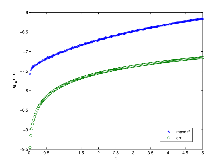
An alternative test of the numerical precision is provided by conserved quantities as the energy,

(3.3)

E=const\int_{-\infty}^{\infty}(2u^{3}-\epsilon^{2}u_{x}^{2})dx.

This quantity is analytically conserved during time evolution, but numerically it will be a function of time due to unavoidable numerical errors. Since energy conservation is not implemented in the code, it provides a strong test for the numerical accuracy. We define the function err via

(3.4)

\mbox{err}:=1-E(t)/E(0),

where $E(t)$ is the numerically calculated energy which is obtained from the first component of the FFT of the integrand in (3.3) at each time step. For the example of the 1-soliton solution, this function is shown in Fig. 9. It can be seen that the error obtained via the integral quantity is typically an order of magnitude higher than the maximal local difference of the exact and the numerical solution. In cases where no exact solution is known, we will use energy conservation as an indicator of the precision of the numerical solution. The number of modes and the time step will be chosen in a way that the value of the function err is at least an order of magnitude lower than the precision of the numerical solution we are aiming at.

To study the small dispersion limit of KdV solutions, we consider hump-like data of the shape of the 1-soliton for both signs, $u=\pm 1/\cosh^{2}(x)$ . We show plots for the evolution of negative initial data in Fig. 10

and for positive initial data in Fig. 11 for $\epsilon=0.1$ and $t\in[0,0.4]$ .

To show that the form of the oscillations for positive and negative initial data is typical, we consider the evolution of the initial data $u=2\sinh(x)/\cosh^{3}(x)$ at time $t=0.4$ for $\epsilon=0.1$ in Fig. 12.

For a given value of $\epsilon$ we need a spatial resolution $2\pi L/N$ of at least $\epsilon$ . We generally try to be an order of magnitude below this limit. Since we use an explicit method for the time integration, stability is an important issue. We find empirically that a time step smaller than $1/N$ leads to a stable time evolution. In Table 1 we give the parameters used in the numerical computations and the obtained numerical errors for different values of $\epsilon$ . We note that the code is very efficient. Up to values of $\epsilon=10^{-3}$ the code can be run on standard computers without problems.

$-\log_{10}\epsilon$	$\log_{2}N$	$L$	$\Delta t$	$\log_{10}\mbox{err}$
1	10	5	$4*10^{-4}$	-6.32
1.25	12	5	$2*10^{-4}$	-7.79
1.5	12	5	$2*10^{-4}$	-6.33
1.75	14	5	$10^{-4}$	-6.30
2	14	5	$5*10^{-5}$	-6.29
2.25	16	4	$2.5*10^{-5}$	-6.30
2.5	16	4	$2.5*10^{-5}$	-4.79
2.75	17	4	$6.67*10^{-6}$	-6.16
3	17	4	$6.67*10^{-6}$	-4.68

Table 1. Parameters used in the numerical integration of the KdV equation for several values of

\epsilon

4. Numerical solution of the Whitham equations and of the Hopf equation

In this section we solve numerically the Whitham equations (2.3) for given initial data by inverting the hodograph transform (2.11) to obtain $\beta_{1}>\beta_{2}>\beta_{3}$ as a function of $x$ and $t$ . Since the hodograph transform becomes degenerate at the leading and trailing edge we solve the system (2.15) instead of (2.11) to avoid convergence problems. In a similar way we address the implicit solution of the Hopf equation (1.4).

Both sets of equations are of the form

(4.1)

S_{i}(\{y_{i}\},x,t)=0,\quad i=1,\ldots,M,

where the $S_{i}$ denote some given real function of the $y_{i}$ and $x$ , $t$ . The task is to determine the $y_{i}$ in dependence of $x$ and $t$ . To this end we determine the $y_{i}$ for given $x$ and $t$ as the zeros of the function $S:=\sum_{i=1}^{M}S_{i}^{2}$ . This will be done numerically by using the algorithm of [27] which is implemented as the function fminsearch in Matlab. The algorithm provides an iterative approach which converges in our case rapidly if the starting values are close enough to the solution (see below how the starting values are chosen). Generally the iteration is stopped for function values smaller than $10^{-6}$ . For quantitative comparisons we calculate the zeros to the order of machine precision.

The solution $\beta_{1}(x,t)>\beta_{2}(x,t)>\beta_{3}(x,t)$ of the Whitham equations exists for $t>t_{c}$ where $t_{c}$ is the time of gradient catastrophe for the solution of the Hopf equation $u_{t}+6uu_{x}=0$ . We look for a solution of the hodograph transform for $t>\dfrac{\sqrt{3}}{8}$ for a discretized time starting with time $t_{1}$ close to $t_{c}$ . For the moment we suppose that $t<T$ , where $T$ is defined in (2.38). For each fixed time, our strategy to solve (2.11) is the following: First we solve the system (2.16) to obtain the leading edge coordinate $x^{-}(t)$ and

\beta_{1}^{-}(t)>\beta^{-}_{2}(t)=\beta^{-}_{3}(t).

At time $t_{1}$ the starting point for solving numerically (2.16) is given by $x^{-}_{0}\sim x_{c}$ and $\beta_{i}^{0}\sim u_{c}$ . Similarly we solve the equations (2.19) for $x^{+}$ and $\beta_{1}=\beta_{2}$ and $\beta_{3}$ which fixes the interval $[x^{-},x^{+}]$ . This interval is subdivided in a number of points $x_{n}$ , $n=1,\ldots,N_{x}$ . We use the values of the $\beta_{i}$ at point $x_{i-1}$ as starting values for the iteration at point $x_{i}$ . A typical plot is shown in Fig. 8. Since the values of the $\beta_{i}$ change rapidly with $x$ near the leading and the trailing edge, we use a grid with one third of the points located in the vicinity of each of the edges and some wider grid spacing in between. To explore the parameter space in $t$ and $x$ we typically use $N_{x}=30$ , for precision calculations we use $N_{x}=300$ and higher. Additional points for plotting purposes are obtained via cubic interpolation.

For $t\geq T$ , the procedure to solve the Whitham equations remains roughly the same. However we have to take care of the fact that the decreasing part of the initial data contributes to the solution of the Whitham equations when $\beta_{3}$ goes beyond the minimum value $-1$ . Thus for $t>T$ we determine the value $x_{T}$ where $\beta_{3}=-1$ as a solution of (2.11). For $x>x_{T}$ we add the contributions of the decreasing part of the initial data. Since the algorithm [27] varies the values of the $\beta_{i}$ for fixed $x$ , one has to make sure for values of $x$ near $x_{T}$ that the right branch of the logarithms is chosen.

The functions (2.11) evaluated in the zero-finding algorithm contain elliptic integrals and integrals over the initial data which are calculated with a Chebychev collocation method. Elliptic integrals and functions are distributed with MATLAB where they are calculated with the algebro-geometric mean (see [1]) to machine precision. We use here the approach to hyperelliptic functions via a Chebychev collocation method presented in [16] (see also Chap. 6 of [24]). The elliptic integrals and functions can be calculated to machine precision with this approach which is checked via internal tests and a comparison with the functions calculated with MATLAB. The reasons for the use of the Chebychev method are twofold. First we can apply similar techniques to calculate the non-standard integrals in (2.11) with machine precision. And secondly we develop in this way an approach to the one-phase Whitham equation which is directly open to a generalization to the multi-phase Whitham equations since the Chebychev code can handle hyperelliptic Riemann surfaces of in principle arbitrary genus.

Let us briefly summarize the Chebychev approach, for details see [16, 24, 6, 15]. The Chebyshev polynomials $T_{n}(x)$ are defined on the interval $I=[-1,1]$ by the relation

T_{n}(\cos(t))=\cos(nt)\;,\mbox{where }x=\cos(t)\;,\qquad t\in[0,\pi]\;.

The addition theorems for sine and cosine imply the recursion relation

(4.2)

\frac{T^{\prime}_{n+1}(x)}{n+1}-\frac{T^{\prime}_{n-1}(x)}{n-1}=2T_{n}(x)

for their derivatives. The Chebyshev polynomials are orthogonal on $I$ with respect to the hermitian inner product

\left<f,g\right>=\int_{-1}^{1}f(x)\bar{g}(x)\,\frac{\mathrm{d}x}{\sqrt{1-x^{2}}}\;.

We have

(4.3)

\left<T_{m},T_{n}\right>=c_{m}\frac{\pi}{2}\,\delta_{mn}

where $c_{0}=2$ and $c_{l}=1$ otherwise. A function $f$ on $I$ is approximated via Chebychev polynomials, $f\approx\sum_{n=0}^{N}a_{n}T_{n}(x)$ where the spectral coefficients $a_{n}$ are obtained by the conditions $f(x_{l})=\sum_{n=0}^{N}a_{n}T_{n}(x_{l})$ , $l=0,\ldots,N$ . This approach is called a collocation method. If the collocation points are chosen to be $x_{l}=\cos(\pi l/N)$ , the spectral coefficients follow from $f$ via a Discrete Cosine Transform for which fast algorithms exist.

The fact that $f$ is approximated globally by a finite sum of polynomials allows us to express any operation applied to $f$ approximately in terms of the coefficients. Let us illustrate this in the case of integration. So we assume that $f=p_{N}=\sum_{n=0}^{N}a_{n}T_{n}$ and we want to find an approximation of the integral for $p_{N}$ , i.e., the function

F(x)=\int_{-1}^{x}f(s)\,\mathrm{d}s\;,

so that $F^{\prime}(x)=f(x)$ . We make the ansatz $F(x)=\sum_{n=0}^{N}b_{n}\,T_{n}(x)$ and obtain the equation

F^{\prime}=\sum_{n=0}^{N}b_{n}\,T^{\prime}_{n}=\sum_{n=0}^{N}a_{n}T_{n}=f\;.

Expressing $T_{n}$ in terms of the $T^{\prime}_{n}$ via (4.2) and comparing coefficients we get the equations

b_{1}=\frac{2a_{0}-a_{2}}{2}\;,\qquad b_{n}=\frac{a_{n-1}-a_{n+1}}{2n}\quad\mbox{for }0<n<N\;,\qquad b_{N}=\frac{a_{N-1}}{2N}\;.

between the coefficients which determine all $b_{l}$ in terms of the $a_{n}$ except for $b_{0}$ . This free constant is determined by the requirement that $F(-1)=0$ which implies (because $T_{n}(-1)=(-1)^{n}$ )

b_{0}=-\sum_{n=1}^{N}(-1)^{n}b_{n}\;.

From the coefficients $b_{n}$ we can also find an approximation to the definite integral $\int_{-1}^{1}f(s)\,\mathrm{d}s=F(1)$ by evaluating

q_{N}(1)=\sum_{n=0}^{N}b_{n}=2\sum_{l=0}^{\lfloor N/2\rfloor}b_{2l+1}\;.

Thus to find an approximation of the integral of a function $f$ we proceed as described above, first computing the coefficients $a_{n}$ of $f$ , computing the $b_{n}$ and then calculating the sum of the odd coefficients.

There are two types of integrals in (2.11). Integrals of the form

(4.4)

\int_{a}^{b}\frac{f(\mu)d\mu}{\sqrt{\mu-a}}

are calculated with the Chebychev integration routine after the transformation $\mu=a+(b-a)(1+y)^{2}/4$ where $y\in I$ . The reason for this transformation is to obtain a smooth integrand free of square roots which is important for an efficient use of spectral methods. After the square root substitution we map the integration to the interval $I$ with a linear transformation. The second type of integral is of the form

(4.5)

\int_{-1}^{1}\frac{f(\nu)d\nu}{\sqrt{1-\nu^{2}}}.

This integral is calculated by expanding the function $f$ in terms of Chebychev polynomials and by using the orthogonality relation (4.3). The precision of the numerical calculation is controlled via test integrals of known functions and via the spectral coefficients: the latter have to be of the order of machine precision for $n\sim N$ to provide sufficient resolution. In our examples 32 to 128 polynomials were always sufficient to fulfill this requirement. Note that there are problems with the integrands if $\beta_{3}\sim-1$ since the $f_{\pm}$ diverge there. This would require an additional coordinate transformation to obtain a smooth integrand necessary for an efficient spectral approximation. Here we are, however, able to perform the required integration by hand. This has the additional benefit to provide a faster code, but the method is able to handle general initial data of the considered form.

To obtain a solution of the Hopf equation we choose again a convenient numerical grid in $t$ and $x\in[x_{L},x_{R}]$ , where $x_{L}$ and $x_{R}$ are $x$ -values where the solution is single valued. We solve equation (1.4) for fixed $t$ and all corresponding values of $x$ starting from $x_{L}$ to $x^{-}$ with starting value $\xi=x$ as described above. Successively we repeat the procedure for greater values of $x_{i}$ on the grid with starting value $\xi_{i-1}$ , the value of $\xi$ found in the preceding step. We find that this approach works well even for $x=x^{-}$ very close to the point of gradient catastrophe $x_{c}$ . Similarly we solve the Hopf equation starting from $x_{R}$ to $x^{+}$ , the $x$ -coordinate of the trailing edge. The solution of the Hopf equation in the region where it is multivalued, is obtained in Fig. 13 by plotting the contour of zero values of the function $x-6tu\pm\ln((1+\sqrt{1+u})/\sqrt{-u})$ . It can be seen form Fig. 13 that the matching of the solution to the Whitham equations to the solution of the Hopf equation is always $C^{1}$ , but the solution of the latter in the multivalued region does not coincide with the former.

The Whitham zone grows in time as can be seen from Fig. 7.

To sum up we have shown in this section that we are able to obtain the numerical solution of the Whitham equations and the asymptotic approximation to the small dispersion limit of the KdV equation with machine precision. The given method is in principle open to deal with general hump-like data with a single minimum. A generalization to a higher genus situation appears to be straight forward. Numerical solutions of the Whitham equations in the genus two case has been obtained in [22] for the Benjamin-One equation.

5. Comparison of the small dispersion KdV solution and its approximation

In the previous sections we have shown how to obtain numerical solutions to the KdV equation in the small dispersion limit as well as the asymptotic solution (1.5) which follows from the solution of the Whitham equations, both with controlled precision. This enables us to present a quantitative comparison of the KdV solution and the asymptotic approximation for several values of the dispersion parameter $\epsilon$ . The code works for general rapidly decreasing initial data with a single hump, for positive initial data, see Fig. 14. This shows numerically that the formula for the phase in Theorem 2.2, which was originally obtained only for negative initial data, can also be used for positive initial data.

In the following we will study as an example the initial data

u_{0}(x)=-\dfrac{1}{\cosh^{2}x}.

The quality of the numerics allows to reach values of $\epsilon$ of the order of $10^{-3}$ without problems. For small $\epsilon$ the asymptotic approximation is almost identical to the KdV solution in the Whitham zone as can be seen in Fig. 5. Thus for small $\epsilon$ it makes little sense to plot both solutions in one figure as in Fig. 2 for $\epsilon=10^{-1}$ . We show the envelope of the asymptotic solution (1.5) and the solution (1.4) together with the solution of the KdV equation in Fig. 15. The shape of the envelope follows from (2.31) to be given by $\beta_{1}-\beta_{2}+\beta_{3}$ and $\beta_{1}+\beta_{2}-\beta_{3}$ .

The numerical precision enables us to study quantitatively the difference between the KdV solution and the asymptotic solutions (1.5) and (1.4) and to establish where the approximation is satisfactory and where it is not. We show this difference for various values of $\epsilon$ in Fig. 16 at time $t=0.4$ .

From Fig. 16 and Fig. 6, it is clear that the error is decreasing with $\epsilon$ . Indeed in the first plot, the highest peak is of the order of $0.15$ , while in the last plot it is of the order $0.06$ . It is also obvious that the asymptotic formula (1.5) gives a satisfactory description of the oscillations within an interval in the Whitham region $[x^{-}(t),x^{+}(t)]$ . At the boundaries of this zone, the highest peaks in the difference appear.

A similar behavior can be observed for the asymptotic solution (1.4). The smaller $\epsilon$ , the better the approximation, which is always worst at the boundary of the Whitham zone. It is also clear that there are in any case oscillations of the KdV solution for values of $x<x^{-}(t)$ for $t>t_{c}$ whereas the solution (1.4) of the Hopf equation, which is considered as an approximation there, obviously does not show any oscillations. As can be seen from Fig. 16, this oscillatory zone shrinks when $\epsilon$ becomes smaller. For values of $x>x^{+}(t)$ , no oscillations are observed but the difference between the KdV solution and the solution (1.4) is biggest at the boundary of the Whitham zone and goes asymptotically to zero. The zone where the solutions differ considerably also shrinks with decreasing $\epsilon$ . Below we will study these features in more detail.

We will present certain characteristic quantities as the difference between the exact and the approximative solution in dependence of $\epsilon$ and show loglog-plots of these quantities. If appropriate we perform a linear regression analysis to identify a scaling behavior in $\epsilon$ of the studied quantity. We briefly summarize the basic relations for a linear regression (see e.g. [2]). Given a set of real points $y_{i}$ , $z_{i}$ with $i=1,..,M$ , we perform a least square fitting to the line $y=az+b$ where with ( $\bar{z}$ , $\bar{y}$ are the mean values)

(5.1)

s_{zz}=\sum_{i=1}^{M}(z_{i}-\bar{z})^{2},\quad s_{zy}=\sum_{i=1}^{M}(z_{i}-\bar{z})(y_{i}-\bar{y}),\quad s_{yy}=\sum_{i=1}^{M}(y_{i}-\bar{y})^{2},

the parameters $a$ and $b$ are given by

(5.2)

b=\frac{s_{zy}}{s_{zz}},\quad a=\bar{y}-b\bar{z}.

For the correlation coefficient being a measure of the quality of the fitting, and the for the standard errors of $a$ and $b$ one has

(5.3)

r=\frac{s_{zy}}{\sqrt{s_{zz}s_{yy}}},\quad\sigma=\sqrt{\frac{s_{yy}-bs_{zy}}{M-2}},\quad\sigma_{a}=\sigma\sqrt{\frac{1}{M}+\frac{\bar{z}^{2}}{s_{zz}}},\quad\sigma_{b}=\frac{\sigma}{\sqrt{s_{zz}}}.

We will only present the results of linear regression if the correlation coefficient is at least of the order of $0.99$ . Even in these cases the results have to be taken with care. We only use a small number of points, but more importantly, we only study values of $\epsilon$ between $10^{-1}$ and $10^{-3}$ . Thus these plots show a scaling law in this regime. Further analytical work will have to show whether these results hold for more general values of $\epsilon$ , and what are the precise values of the coefficients.

Whitham zone

From Fig. 16 and Fig. 6 it is obvious that the asymptotic approximation (1.5) does not give a satisfactory description of the KdV solution close to the boundary. However one can identify an interior zone where this approximation gives a rather accurate description of the KdV zone. There is an obvious arbitrariness in the definition of such an interior zone since the difference between KdV solution and approximation is not constant there. As can be seen from Fig. 17 there is also an error in the phase. Close to $x=-2.5$ the KdV solution and the asymptotic solution are in phase, and consequently the difference is minimal there.

A possible definition of the interior zone is simply to cut off the big oscillations at the edges. If one cuts off just one full oscillation, the cut off zone scales roughly like $\epsilon$ in accordance with the fact that there are oscillations of the order $1/\epsilon$ in the Whitham zone. For the case $t=0.4$ and $\epsilon=10^{-3}$ , we obtain Fig. 17.

To define an error ( $\mbox{err}_{mid}$ ) in the interior we take the maximum of the absolute value of the difference between the solutions in the vicinity of the center of the zone ( $x\approx-2.66$ ). Notice that there is a certain crudeness in this definition of the error since this maximum will occur for different $\epsilon$ at slightly different values of $x$ . Because of the error in the phase there are large differences in the error for different $\epsilon$ if one takes the difference at the same $x$ value in all cases. The so defined error is shown in Fig. 18, where it can be seen that it decreases almost linearly with $\epsilon$ . Linear regression analysis yields $a=1.0049$ , $b=0.1005$ with $\sigma_{a}=0.05$ , $\sigma_{b}=0.024$ , and a correlation coefficient $r=0.998$ .

The maximal error near the boundaries of the Whitham zone is shown in Fig. 19. There seems to be no obvious scaling of these errors with $\epsilon$ which is probably due to the rapid oscillations of the error because of the error in the phase.

Oscillatory zone with $x<x^{-}(t)$

As can be seen in Fig. 5 and Fig. 6, there are always oscillations of the KdV solution for $t>t_{c}$ which do not occur for the asymptotic solution (1.4). We show this region in detail in Fig. 20.

It can be seen that the oscillatory zone clearly shrinks with decreasing $\epsilon$ . There is no obvious rigorous definition of the end of the oscillatory zone. The difference will eventually be of the order of the numerical error for the KdV solution. We define the end of the oscillatory zone as the $x$ -value where the amplitude of the difference of the solutions is smaller than $10^{-4}$ which is of the order of the numerical accuracy we have used. The width of this zone, $\Delta_{hopf}^{-}:=x_{hopf}^{-}/x^{-}-1$ in dependence of $\epsilon$ is shown in Fig. 21. It can be seen that the oscillatory zone shrinks to zero with $\epsilon$ . Asymptotically the boundary of this zone approaches the boundary of the Whitham zone. We find that $\Delta_{hopf}^{-}$ scales roughly as $\epsilon^{3/4}$ . The linear regression analysis yields $a=0.761$ and $b=-0.789$ with $\sigma_{a}=0.028$ , $\sigma_{b}=0.013$ and $r=0.999$ . However, this result has to be taken with care in view of the low number of points and the arbitrariness in the definition of the zone.

The error $\mbox{err}_{hopf}^{-}$ in this zone is measured by the maximum of the absolute value of the difference of the amplitude between the KdV solution and the Hopf solution. This maximum value always occurs close to the boundary of the Whitham zone. The error $\mbox{err}_{hopf}^{-}$ is shown in Fig. 22. It decreases roughly as $\epsilon^{1/3}$ . Linear regression analysis yields $a=0.346$ , $b=0.250$ with $\sigma_{a}=0.025$ , $\sigma_{b}=0.012$ and $r=0.996$ .

Zone with $x>x^{+}(t)$

A similar behavior is found in the zone for $x>x^{+}(t)$ with the exception that there are no oscillations. The difference of the asymptotic solution (1.4) and the KdV solution is biggest for $x^{+}(t)$ and decreases monotonically to the order of the numerical precision.

We define the width of the zone as the region where the absolute value of the difference is bigger than $10^{-4}$ . The values of the quantity $\Delta_{hopf}^{+}:=1-x_{hopf}^{+}/x^{+}$ are shown in Fig. 24 in dependence on $\epsilon$ . It can be seen that this zone shrinks with $\epsilon$ to zero, i.e., its boundary approaches asymptotically the boundary of the Whitham zone. Apparently there is no simple $\epsilon$ -dependence of this quantity, at least not for the number of points used in the plot.

The maximal error in this zone always occurs at the boundary to the Whitham zone. As can be seen in Fig. 25, this error decreases roughly as $\sqrt{\epsilon}$ . Linear regression analysis yields $a=0.525$ , $b=0.554$ with $\sigma_{a}=0.017$ , $\sigma_{b}=0.008$ and $r=0.999$ .

Breakup time

As discussed above the asymptotic approximation of the small dispersion KdV solution is always worst near the boundary of the Whitham zone. At the breakup time $t_{c}$ being defined as the time of gradient catastrophe of the solution to the Hopf equation, the Whitham zone consists only of one point. In Fig. 3 it can be seen that the solution to the KdV equation always forms oscillation for times $t<t_{c}$ . Thus the first oscillation in the Whitham zone gives only a very crude approximation to the oscillation of the KdV solution in this zone. In addition there are typically several oscillation of the KdV solution outside the Whitham zone at this time. The discrepancy between the asymptotic and the KdV solution is quite pronounced even for small $\epsilon$ as can be seen from Fig. 26 for $\epsilon=10^{-3}$ . The KdV solution develops roughly the same number of oscillations before $t_{c}$ as in Fig. 3, but on a smaller scale. As already stated, the oscillatory zone shrinks with decreasing $\epsilon$ , but close to the breakup the difference between the asymptotic solutions and the KdV solution remains considerable, even for small $\epsilon$ . As can be seen in Fig. 27, the difference between asymptotic solution and KdV solution is biggest close to the breakup time.

Time dependence

The qualitative behavior of the difference of the small dispersion KdV solution and the asymptotic solution as outlined above is characteristic for all times as can be seen from Fig. 27.

The difference is always biggest at the boundary of the Whitham zone. The absolute value of this difference is almost constant in time at the boundary. Therefore the discrepancy between the approximation and the solution is biggest close to breakup. The interior zone where the asymptotic solution gives a very satisfactory approximation grows with time.

6. Outlook

In this paper we have presented a quantitative numerical treatment of the solution to the KdV equation in the small dispersion limit for initial data with compact support and a single hump. The same has been achieved for the asymptotic formulas for the same initial data. The code for the KdV solution is set up to handle general initial data with compact support, thus the inclusion of initial data which develop multi-phase solutions is directly possible. The approach to the solution of the one-phase Whitham equations is also open to a generalization to multi-phase case. In particular the existence and uniqueness of the solution of the two-phase Whitham equations has been obtained in [17] for generic initial data where $f_{-}$ has negative fifth derivative. Since the Chebychev code [16, 24] to calculate the characteristic quantities on the elliptic surface in the present paper is able to deal with almost arbitrary hyperelliptic surfaces, the corresponding models can be studied. This will be the subject of future work.

The results of the previous section show that the asymptotic approximation is worst at break up point and at the boundary of the Whitham zone. According to the conjecture in [10],[26] the solution of the KdV equation, near the point of gradient catastrophe, is well described by

(6.1)

u(x,t,\epsilon)=u_{c}+\left(\dfrac{\epsilon}{k}\right)^{2/7}F\left(-\dfrac{1}{\epsilon}\left(\dfrac{\epsilon}{k}\right)^{1/7}(x-x_{c}-6u_{c}(t-t_{c}));\;\dfrac{1}{\epsilon}\left(\dfrac{\epsilon}{k}\right)^{3/7}(t-t_{c})\right),

where

\quad k=-\dfrac{f_{-}^{\prime\prime\prime}(u_{c})}{6},

and the function $F(X;T)$ is the solution of the fourth order ODE of the Painlevé I hierarchy

(6.2)

-6TF+F^{3}+FF^{\prime\prime}+1/2(F^{\prime})^{2}+1/10F^{\prime\prime\prime\prime}=X.

The above equation first appeared in the double scaling limits of one matrix models for the multicritical index $m=3$ and for $T=0$ [4]. It is conjectured that the equation (6.2) has a smooth real solution on the real line with asymptotic behavior $F(X,0)=\pm X^{\frac{1}{3}}$ for $X\rightarrow\pm\infty$ . We will investigate numerically the asymptotic description given by (6.1) in a subsequent publication.

The description of the left oscillatory zone outside the Whitham zone, should be obtained in the spirit of matrix models, performing a sort of double scaling limit. According to the ansatz in [26], the envelope of the oscillations is given by the Hastings McLeod solution of the second Painlevé equation. This result is in accordance with the rigorous results obtained in the double scaling limit in one-matrix models [9],[5],[7].

Regarding the right boundary of the Whitham zone, at the moment, there is no theoretical ansatz for an asymptotic description. Our numerical results could possibly provide a hint for an ansatz for the asymptotic behavior.

It would also be very interesting to perform similar numerical investigations for the semiclassical limits of the focusing [23] and defocusing [21] nonlinear Schrödinger equation.

References

[1] M. Abramowitz and I. A. Stegun, Handbook of Mathematical Functions, Dover Publications, 1965, 17.6.
[2] F. S. Acton, Analysis of Straight-Line Data, New York: Dover, 1966.
[3] V. V. Avilov, S. P. Novikov, Evolution of the Whitham zone in KdV theory, Soviet Phys. Dokl., 32:366-368 (1987).
[4] E. Brézin, E. Marinari, G. Parisi, A nonperturbative ambiguity free solution of a string model. Phys. Lett. B 242 (1990), no. 1, 35–38.
[5] P. Bleher, A. Its, Double scaling limit in the random matrix model: the Riemann-Hilbert approach. (English. English summary) Comm. Pure Appl. Math. 56 (2003), no. 4, 433–516.
[6] C. Canuto, M. Y. Hussaini, A. Quarteroni and T.’ A. Zang, Spectral Methods in Fluid Dynamics, Springer-Verlag, Berlin, 1988.
[7] T. Claeys, A. B. J. Kuijlaars, M. Vanlessen, Multi-critical unitary random matrix ensembles and the general Painleve II equation, preprint xxx.lanl.gov/math-ph/0508062.
[8] P. Deift, S. Venakides and X. Zhou, New result in small dispersion KdV by an extension of the steepest descent method for Riemann-Hilbert problems, IMRN 1997 6 285-299.
[9] P. Deift, T. Kriecherbauer, K. T.-R. McLaughlin, S. Venakides, X. Zhou, Uniform asymptotics for polynomials orthogonal with respect to varying exponential weights and applications to universality questions in random matrix theory. (English. English summary) Comm. Pure Appl. Math. 52 (1999), no. 11, 1335–1425.
[10] B. Dubrovin, On Hamiltonian perturbations of hyperbolic systems of conservation laws, II: universality of critical behaviour, preprint, http://xxx.lanl.gov/math-ph/0510023.
[11] B. Dubrovin, S. P. Novikov, A periodic problem for the Korteweg-de Vries and Sturm-Liouville equations. Their connection with algebraic geometry. Dokl. Akad. Nauk SSSR 219 (1974), 531–534.
[12] B. Dubrovin, S. P. Novikov, Hydrodynamic of weakly deformed soliton lattices. Differential geometry and Hamiltonian theory, Russian Math. Surveys 44:6, 35-124 (1989).
[13] G. A. El, A. Krylov, S. Venakides, Unified approach to KdV modulations, Comm. Pure Appl. Math. 54 (2001), no. 10, 1243–1270.
[14] H. Flaschka, M. Forest, and D. H. McLaughlin, Multiphase averaging and the inverse spectral solution of the Korteweg-de Vries equations, Comm. Pure App. Math. 33:739-784 (1980).
[15] B. Fornberg: A practical guide to pseudospectral methods, (Cambridge University Press, Cambridge 1996)
[16] J. Frauendiener and C. Klein, ‘Hyperelliptic theta functions and spectral methods’, J. Comp. Appl. Math., Vol. 167, 193 (2004).
[17] T. Grava, Fei-Ran Tian, The generation, propagation, and extinction of multiphases in the KdV zero-dispersion limit. Comm. Pure Appl. Math. 55 (2002), no. 12, 1569–1639.
[18] T. Grava, From the solution of the Tsarev system to the solution of the Whitham equations. Math. Phys. Anal. Geom. 4 (2001), no. 1, 65–96.
[19] A. G. Gurevich, L. P. Pitaevskii, Non stationary structure of a collisionless shock waves, JEPT Letters 17:193-195 (1973).
[20] A. Its, V.B.Matveev, Hill operators with a finite number of lacunae. (Russian) Funkcional. Anal. i Priložen. 9 (1975), no. 1, 69–70.
[21] Shan Jin, D. Levermore, D.W. McLaughlin, The semiclassical limit of the defocusing NLS hierarchy. Comm. Pure Appl. Math. 52 (1999), no. 5, 613–654.
[22] M.C. Jorge, A.A.Minzoni, N.F.Smyth, Modulation solutions for the Benjamin-Ono equation. Phys. D 132 (1999), no. 1-2, 1–18.
[23] S. Kamvissis, K. D. T.-R. McLaughlin, P. D. Miller, Semiclassical soliton ensembles for the focusing nonlinear Schrödinger equation. Annals of Mathematics Studies, 154. Princeton University Press, Princeton, NJ, 2003.
[24] C. Klein and O. Richter ‘Ernst Equation and Riemann Surfaces’, Lecture Notes in Physics 685 (Springer) (2005).
[25] I. M. Krichever, The method of averaging for two dimensional integrable equations, Funct. Anal. Appl. 22:200-213 (1988).
[26] V. Kudashev, B. Suleimanov, A soft mechanism for the generation of dissipationless shock waves, Physics Letters A 221 (1996) 204-208.
[27] J. C. Lagarias, J. A. Reeds, M. H. Wright, and P. E. Wright, Convergence Properties of the Nelder-Mead Simplex Method in Low Dimensions, SIAM Journal of Optimization, Vol. 9 Number 1, pp. 112-147, 1998.
[28] D. F. Lawden, Elliptic functions and applications. Applied Mathematical Sciences, 80. Springer-Verlag, New York, 1989.
[29] P. D. Lax and C. D. Levermore, The small dispersion limit of the Korteweg de Vries equation,I,II,III, Comm. Pure Appl. Math. 36:253-290, 571-593, 809-830 (1983).
[30] C.D. Levermore, The hyperbolic nature of the zero dispersion KdV limit. Comm. Partial Differential Equations 13 (1988), no. 4, 495–514.
[31] D. W. McLaughlin, J. A. Strain, Computing the weak limit of KdV. Comm. Pure Appl. Math. 47 (1994), no. 10, 1319–1364.
[32] Fei-Ran Tian, Oscillations of the zero dispersion limit of the Korteweg de Vries equations, Comm. Pure App. Math. 46:1093-1129 (1993).
[33] Fei-Ran Tian, The initial value problem for the Whitham averaged system. Comm. Math. Phys. 166 (1994), no. 1, 79–115.
[34] L. N. Trefethen, Spectral Methods in MATLAB, SIAM, Philadelphia, PA, 2000.
[35] S. P. Tsarev, Poisson brackets and one-dimensional Hamiltonian systems of hydrodynamic type, Soviet Math. Dokl. 31:488-491 (1985).
[36] S. Venakides, The zero dispersion limit of the Korteweg de Vries equation for initial potential with nontrivial reflection coefficient, Comm. Pure Appl. Math. 38 (1985) 125-155.
[37] S. Venakides, The Korteweg de Vries equations with small dispersion: higher order Lax-Levermore theory, Comm. Pure Appl. Math. vol. 43, 335-361, 1990.
[38] G. B. Whitham, Linear and nonlinear waves, J.Wiley, New York, 1974.
[39] www.comlab.ox.ac.uk/oucl/work/nick.trefethen

Abstract.

1. Introduction

2. Lax Levermore theory and Whitham equations

2.1. The Cauchy problem for the Whitham equations

Theorem 2.1.

Theorem 2.2.

Proof.

Theorem 2.3.

Proof.

2.2. The explicit example

3. Numerical solution of the KdV equation

4. Numerical solution of the Whitham equations and of the Hopf equation

5. Comparison of the small dispersion KdV solution and its approximation

Whitham zone

Oscillatory zone with x<x−​(t)x<x^{-}(t)

Zone with x>x+​(t)x>x^{+}(t)

Breakup time

Time dependence

6. Outlook

References

Oscillatory zone with $x<x^{-}(t)$

Zone with $x>x^{+}(t)$