A Contour Integral Representation for the Dual Five-Point Function and a Symmetry of the Genus Four Surface in
Abstract
The invention of the “dual resonance model” -point functions motivated the development of current string theory. The simplest of these models, the four-point function , is the classical Euler Beta function. Many standard methods of complex analysis in a single variable have been applied to elucidate the properties of the Euler Beta function, leading, for example, to analytic continuation formulas such as the contour-integral representation obtained by Pochhammer in 1890. However, the precise features of the expected multiple-complex-variable generalizations to have not been systematically studied. Here we explore the geometry underlying the dual five-point function , the simplest generalization of the Euler Beta function. The original integrand defining leads to a polyhedral structure for the five-crosscap surface, embedded in , that has 12 pentagonal faces and a symmetry group of order 120 in . We find a Pochhammer-like representation for that is a contour integral along a surface of genus five in . The symmetric embedding of the five-crosscap surface in is doubly covered by a corresponding symmetric embedding of the surface of genus four in that has a polyhedral structure with 24 pentagonal faces and a symmetry group of order 240 in . These symmetries enable the construction of elegant visualizations of these surfaces. The key idea of the paper is to realize that the compactification of the set of five-point cross-ratios forms a smooth real algebraic subvariety that is the five-crosscap surface in . It is in the complexification of this surface that we construct the contour integral representation for . Our methods are generalizable in principle to higher dimensions, and therefore should be of interest for further study.
1 Introduction
Historical Background.
In 1968, Gabriele Veneziano [18] noticed that an amazing number of abstract properties required by the relativistic scattering amplitude for four colliding spinless particles were embodied in the classical Euler Beta function, , which can be defined by the integral representation
| (1) |
This observation served as the implausible origin of modern string theory (see, e.g., [13, 14] for more details), which grew from the discovery that the Beta function could be related to the vibration modes of a relativistic string sweeping out a surface in spacetime [11, 4].
Almost immediately following Veneziano’s discovery, a function with a two-dimensional integral representation was found that could be related to the relativistic scattering amplitude of five spinless particles [1, 19]. This function, the dual five-point function , can be written in various representations such as the following integral over a triangular region
| (2) | |||||
for suitably restricted values of the arguments . The discovery of this function indicated that the Euler Beta function was not alone: the Euler Beta function, which would now be written as , was henceforth to be regarded as the first member of the family of -point functions that might be expected to have interesting properties in analysis as well as in the quantum theory of relativistic elementary particles.
Cross-Ratio Coordinates.
A very rapid series of steps subsequently led to what became the standard Koba-Nielsen representation [10] for the -point function , which can be written as an -dimensional integral
| (3) |
where and the are the -point cross-ratios parameterized by as described in detail in Section 2. The formulas (1) and (2) correspond to (3) for the cases and , respectively.
A variety of methods have been employed to study the properties of the integrands as functions of complex variables. For example, Koba and Nielson [10] expressed (3) as an integral in a space that was essentially a product of copies of . As noted by one of the current authors in [6], one can alternatively express the complex integrand by employing cross-ratios (with a much larger symmetry group) in place of the product of complex projective lines with the single shared linear fractional transformation symmetry characterizing the Koba-Nielsen framework.
We will see in the following that, for , the compactification of the set of all five-point cross-ratios can be identified with as an algebraic subvariety in with a polyhedral structure that has 12 pentagonal faces. This embedding of has a symmetry group of order 120 in . The double covering, which is the surface of genus four embedded in , has a corresponding polyhedral structure with 24 pentagonal faces and a symmetry group of order 240 in . The integral (2) is taken over one of the 12 pentagonal faces of . This is the starting point for the contour integral representation of .
The study of such a tessellation on , the five crosscap surface, and its symmetry group dates back to the 19th century [9] and is treated in detail in the work of Brahana and Coble in 1926 [2]. It is interesting to see that our space of five-point cross-ratios leads naturally to the same tessellation, and to the presentation of the symmetry group in .
Contour Integral Representations.
It is well known that the analytic continuation of the function defined by (1) is a meromorphic function of on the entire complex space . In fact, changing variables in the integral allows the Beta function to be rewritten in terms of the standard integral representation of the Gamma function, leading to the explicit analytic continuation formula
| (4) |
In 1890, Pochhammer [12] gave another interesting continuation formula for in the following form,
| (5) |
where is a contour integral of along a properly immersed loop in , and hence is a holomorphic function of .
Our observation that the function can be expressed by an integral over one pentagonal face of leads to a contour integral representation analogous to Pochhammer’s classic representation of . We obtain the following two-dimensional contour integral representation of :
| (6) | |||||
Here is a holomorphic function expressed as an integral of a holomorphic 2-form along a closed oriented surface of genus 5 properly immersed in . Note that, unlike the representation (2), where must be properly restricted for the integral to be convergent, the representation (6) of is a meromorphic function of and is defined on the entire space . Hence the formula (6) is an explicit analytic continuation formula for the five-point function originally defined by (2).
We point out that, to produce the required contour for , not only is the two-complex-variable environment supplied by the Koba-Nielson product of two projective lines, , inadequate, but the richer alternative framework of [6] is also inadequate. The contour lies instead in , which is the complexification of the above-mentioned five-crosscap surface in considered as the real part of .
We begin in Section 2 by introducing the -point cross-ratio, which gives rise to the subvarieties upon which our analysis is based. Section 3 constructs the 12-pentagon tessellation of the five-crosscap surface as the compactification of the set of 5-point cross-ratios; its symmetries and the genus-four double cover are given in Section 4. Then, in Section 5, we review Pochhammer’s classical construction for the contour integral representation of the Euler Beta function. The framework for studying is set up in Section 6 where the representation (6) is proven. Selected constructions are applied to visualizations and computer graphics representations of the relevant structures in Section 7. Remarks on the extension to general are presented in Section 8.
2 Cross-Ratios
Recall that the cross-ratio of four distinct ordered numbers is defined as
| (7) |
For any integer , we define the -point cross-ratio of a cyclically-ordered set of distinct numbers as the ordered set of numbers , where
| (8) |
and , .
The set of all -point cross-ratios can be considered as a subset of , which we denote by . From the well-known fact that the cross-ratio is invariant under linear fractional transformations of , it is clear that can be parameterized by variables, which we denote as . That is, each point of is the -point cross-ratio of the cyclically ordered numbers
| (9) |
for a unique , where are distinct and not equal to 0 or 1.
For example, for , if we set , , , and , then, according to (8), the set of -point cross-ratios in is given by the following parameterized curve:
Notice that there are three connected components for the domain of , as shown in Figure 1.

For , the set of -point cross-ratios is a surface in parameterized by as
| (10) | |||||
The domain of has twelve connected components, as shown in Figure 2.

One can verify that the cross-ratios defined by (8) satisfy
| (11) |
with the convention that and for all . In fact, the affine algebraic subvariety in defined by (11), minus a set of measure zero, is precisely the set of -point cross-ratios.
In particular, for , the constraint (11) becomes
| (12) |
The set is the affine algebraic subvariety in with coordinates given by the linear equation
| (13) |
For , we have
| (14) | |||||
and is the affine algebraic subvariety in with coordinates given by
| (15) | |||||
Remark. It can be verified that the system (15) has rank 3 at the zero locus, and therefore does actually define a smooth algebraic subvariety of dimension 2.
Now consider the corresponding projective subvarieties. For , (13) becomes
| (16) |
which obviously defines a projective line in with homogeneous coordinates .
Similarly, for , (15) yields the following homogeneous quadratic equations in the homogeneous coordinates of :
| (17) | |||||
One can verify that (17) defines a smooth two-dimensional subvariety in , which we will denote by . To see the topology of , we examine the parameterization (10). As we will show in detail in Section 3, the image of each of the twelve connected components of the parameter domain has a smooth pentagonal closure tessellating as shown in Figure 3.

Extending (17) to complex variables defines a complex algebraic variety that is obviously the complexification of the real manifold . is with four points blown up and is topologically homeomorphic to .
The tessellation represented in Figure 3 has 12 pentagonal faces, edges, and vertices; the Euler number of is thus , and therefore is the connected sum of five ’s, i.e., a sphere with five crosscaps. Therefore, viewing the five-crosscap surface as the set of cross-ratios yields a natural tessellation with 12 pentagonal faces, which we can call a “dodecahedron” even though it does not bound a 3-ball. This tessellation was already described in detail from the point of view of combinatorial topology in the 19th century [9]. In 1926, Brahana and Coble [2], also arrived at the same tessellation of a sphere with five crosscaps as a map of 12 countries with five sides, and studied the symmetry group in detail (see also recent work by Weber [20] for additional historical background). Such tessellations were generalized by Stasheff for use in his study of the homotopy theory of H-spaces [15, 16, 17], and, in particular, the analogous tiles in higher dimensions are called associahedra. These have played a prominent role, e.g., in the work of Devadoss [3]. Our discovery of the relation between the five-crosscap dodecahedral tessellation and the 5-point cross-ratios, as well as the apparent relation between the higher-dimensional analogs and the -point cross-ratios, should thus be of further interest.
3 Closure of the 5-Point Cross-Ratio Set in
We now present a detailed treatment of the pentagonal tessellation for . In the homogeneous coordinates of , we will write the parameterization (10) as
| (18) | |||||
On the triangular connected component , as or , the images do not converge to a point. To extend the parameterization to the boundary of the domain, we will replace the parameters as follows.
First, let
| (19) |
The formula (19) defines a 1-1 map between the open square in the -plane and the open triangle in the -plane, as shown in Figure 4.


Next, in Table 1, we present twelve formulas that give 1-1 maps between the open triangular domain and each of the twelve connected components shown in Figure 2.
| n | The map from the region to the connected component in Figure 2. |
|---|---|
| , | |
Composing (18), the entries in Table 1, and (19), we get a parameterization for each of the 12 connected components of on the common domain in the -plane. We will denote these parameterizations by , respectively.
It can be verified that each of the extends as a 1-1 parameterization to the closed square . Each of the twelve images is a smooth, closed, pentagonal surface patch whose vertices correspond to
Examining the pentagons one by one, we find they are joined together to form the closed surface represented by Figure 3.
For future reference, we list below the homogeneous coordinates of the 15 vertices:
| (20) |
4 Symmetries and the Double-Covering Lift
One can see using combinatorial arguments that the tessellation of shown in Figure 3 has many symmetries. We will present the group of symmetries as follows.
One of the symmetries, when restricted to face , is a rotation that transforms the vertices 1,2,3,4,5 to 2,3,4,5,1. This symmetry also transforms vertex 12 to vertex 15. Using the coordinates of these vertices from (20), we construct the matrix
with the matrix given by , where , etc., are written as column vectors whose components are specified by (20). Similarly, , yielding
| (21) |
Another symmetry is the reflection along the edge joining and , which transforms vertices 1,2,3,4,5,12 to 12,7,3,4,9,1. As above, one constructs
| (22) |
The following observations are essential: Viewing and as elements of , one can verify that the zero-locus of (17) is invariant under the corresponding transformations of . and generate a group of order 120, which is isomorphic to the group of automorphisms of mentioned above. In other words, we have embedded the automorphism group of in .
In fact, and generate a subgroup of order 120 in . We let
| (23) |
More explicitly,
| (24) |
As is well-known, defines a -invariant quadratic form on . Then the algebraic subvariety in defined by
| (25) | |||||
is -invariant and we denote it by .
Comparing to (17), we see that is the double covering of lifted from to and is therefore topologically the orientable surface of genus four. Notice that is also invariant under the action of , where denotes the identity matrix. Hence, is invariant under the group generated by , , and , which has 240 elements in .
Let be a matrix satisfying
| (26) |
Then , where is the unit sphere in , and it is invariant under the subgroup of order 240 in generated by , , and .
With the parameterization for from Section 3, we can now easily write down the following parameterization for :
| (27) |
Each maps in the -plane to a pentagonal surface patch. This yields a tessellation of with 24 pentagonal faces. As mentioned at the end of Section 2, such a tessellation for the genus-four surface has long been known. Here we have performed this tessellation symmetrically in .
The coordinates of the vertices appearing in the tessellation of can be computed from (27) at the points . They are in fact the same as those presented in (20), together with their negatives, viewed now as coordinates in .
We now identify the 24 faces in with ordered sets of vertices in : the oriented faces are labeled in terms of the indices of the vertices in (20), where a minus sign indicates the negative mirror vertex and conjugate faces are denoted with bars:
| (28) |
The correspondence between the 12 projective faces and the 12 regions of Figure 2 is shown in Figure 3; the correspondence between the 24 faces in the double cover and the 12 regions is shown in Figure 5.


5 Review of the Pochhammer Contour for B4
In this section, we review Pochhammer’s construction [12, 8, 21] of the contour integral leading to the formula (5) for . This will lead us to the contour integral representation for to be presented in Section 6.
Let
| (29) |
where is a pair of arbitrary complex numbers. Considered as a function of , defines a family of holomorphic functions on a proper Riemann covering sheaf over . Let be a closed and oriented curve in that is the lift of the closed and oriented curve in shown in Figure 6, where we label the line segments by their relative phases in the lift. This is known as the Pochhammer contour.

Next, define
Clearly is a holomorphic function of and is invariant under continuous deformations of . Therefore, letting in Figure 6, one easily sees that, if and , then
which yields the formula (5).
If (or , resp.) is an integer , then the holomorphic 1-form on descends to a holomorphic 1-form on a proper Riemann covering sheaf over (or , resp.). Since the curve in Figure 6 is contractible in (or , resp.), .

Notice that, by letting , we have
This shows that, if is a non-positive integer (), the holomorphic 1-form on descends to a holomorphic 1-form on a proper Riemann covering sheaf over , where as usual we identify with . Since the curve in Figure 6 is contractible in (see Figure 7), it therefore follows that also in this case. Figure 7 shows how the contractibility of the contour can be made explicit.
From these observations and (5), one concludes in particular that the poles of can only occur at points where either or is a non-positive integer. Furthermore, if neither nor is a non-positive integer, but is a non-positive integer. These properties of course also follow directly from (4); in fact these are precisely all the poles and zeroes of .
6 Contour Representation of the Function B5
We now view as the real two-dimensional surface in , as defined at the end of Section 2. The manifold can be visualized by the complexification of Figure 3; with the edges of the pentagon taken off, is now parameterized by two complex parameters that we denote as , replacing in (18). Following the procedure in Section 5, let
| (30) | |||||
Then (2) can be viewed as the integral of the (locally) holomorphic 2-form (with branched singularities) on over the domain on .
The function can be viewed as a 5-complex-parameter family of locally holomorphic functions on with branched singularities at the edges of the pentagons evident in the complexification of Figure 3.
Let be the Riemann covering sheaf of over . We will construct an orientable closed surface in that is the lift of a closed surface in obtained by wrapping properly around the five (complex) edges of the pentagonal domain . This will then lead to the formula (6).
A function such as is only defined on , away from singularities, up to a factor , i.e., by a phase which is an integer linear combination of . To lift a surface wrapping around the branch lines to the covering sheaf , on which is a holomorphic function, we first need to understand how the phase of changes on a piece of surface as it makes a simple fold back around one branch line (see Figure 8).

It is obvious that if a surface folds back around the branch line , , or , then the phase of changes by , , or , respectively, where the sign or depends on the folding direction, i.e., whether the direction is counterclockwise or clockwise.


To see how the the phase of changes on a surface folding around the branch line (see Figure 9), let be the coordinates around chosen so that is given by , and away from , , (cf. [5] and Figure 10). We can then write as
It is now easy to see that as a surface folds back around A, the phase of changes by . Similarly, one can show that as a surface folds back around B, the phase of changes by .
We now construct an immersed surface in in three steps as follows:
- Step 1.
Consider a set of 32 copies of the pentagonal sheets stacked over the region 1 in Figure 9, with a small neighborhood of the five corners taken off for now. From what we have shown above, it is appropriate to label the edges of each pentagonal sheet at by , respectively (see Figure 11).


Figure 11: The pentagonal sheets in region 1. We attach to each of these pentagonal sheets a phase label
where or for . Each pentagonal sheet is given an orientation which is same as or opposite to the original natural orientation on region 1 according to whether is even or odd.
- Step 2.
Two pentagonal sheets in Step 1 are joined along the edge by folding around the corresponding branch line in the proper direction (see Figure 8) if and only if their phase numbers differ by . It is easy to see that we end up with an immersed oriented surface in that can be lifted to . However, this surface has 40 holes caused by the small neighborhoods that we removed around the corners where the branch lines intersect. In Figure 12, we show a single instance of one of these holes.


(a) (b)
Figure 12: (a) The hole at a single corner. (b) A hole-filling disk in enclosing the intersection point of the two (complex) branch lines. - Step 3.
To show that one can fill in these holes, we observe that a small 3-sphere around an intersection of two branch lines, with the branch lines taken off, is homotopic to a torus and hence its fundamental group is isomorphic to the Abelian group . It is easy to see that the boundary of a small hole at this intersection, which lies in the surrounding 3-sphere, represents the element and therefore is contractible (a filled-in disk as illustrated in Figure 12(b)).
Remark: If one tries to construct such a surface directly in , then there would be a hole at a corner where three branch lines intersect, and for such holes the argument above fails.
We have therefore obtained an oriented closed surface immersed in , whose Euler characteristic can be easily seen to be . Hence the surface is of genus 5, i.e., a sphere with five handles.
Now, let
Clearly is a holomorphic function of and is invariant under continuous deformations of . As in the case of the Pochhammer contour described in Section 5, we can take the limit and calculate for suitably restricted that
This proves (6).
Following the analogy to the Pochhammer analysis to determine further constraints on the poles and zeroes of is an interesting challenge for future work.
7 Visualizations of Connected Components and Pochhammer Contours
The analysis of the function in the previous sections has been based entirely on algebraic manipulations and line drawings sketching the essential features of the geometry. This section is motivated by the observation that, since there are algebraic constructions for every geometric concept, we can go one step further and show precise images of each construction, helping the reader to develop a quantitative as well as a qualitative understanding of the framework we have developed. We establish the basic context with some examples based on the Euler Beta function, and then proceed to show some of the remarkable manifolds that occur in the analysis.
7.1 Connected Components Embedded in a Veronese Surface
The Euler Beta function itself can be analyzed using cross-ratio coordinates. We begin with the two cross-ratio variables, and , obeying the apparently uninteresting constraint
However, when we put this into homogeneous coordinates , the constraint becomes , and we can solve these equations independently in the three component regions, written as three intervals in inhomogeneous coordinates as , , and . Noting that the space we are now dealing with is not or , but the real part of the cross-ratio-space, we can parameterize each interval in homogeneous coordinates as follows:
| (31) | |||||
We see that region solves with , solves with when all is multiplied by , and solves with when all is multiplied by . The interpolating functions in the three regions obviously correspond to the three component regions introduced initially in Figure (1), and they interpolate between the points represented in the Riemann-sphere depiction of Figure 13:

But there is a small problem: if we follow the coordinate interpolations carefully, they only work projectively; the actual interpolations close on one another only if we include the negative, projectively-equivalent points , for a total of 6 points and six linear paths, rather than three. Thus, the projective coordinates for the three components can be plotted either as a connected hexagon in , the embedding space of the homogeneous coordinates, or as a more visually consistent projection onto a constant-radius , the double-cover of , as shown in Figure 14(a).

(a)


(b) (c)
To actually achieve the desired end result of a visualization of the cross-ratio coordinates in a logical embedding, we must find a quadratic map that removes the distinction between the positive and negative versions of the same projective coordinates and maps explicitly to . This is achieved classically by the Veronese surface (see, e.g., the traditional embedding of given in the appendix of Hilbert and Cohn-Vossen, [7]):
| (32) |
where the spherical constraint implies the standard Veronese surface constraint . In Figures 14(b) and (c), we see the exact paths of the three component integrals of the Euler Beta function as they are embedded in alternate projections of (the real part of ) to 3D. This is equivalent mathematically, and yet a significantly contrasting viewpoint, to the conventional alternative indicated in Figure 13.
7.2 Visualizing the Pochhammer Contour
We now illustrate explicitly the geometry of the Pochhammer contour for the Euler Beta function. Starting from (29), we choose a pair of small relatively prime rational exponents , and project the 4D plot of to 3D, with the horizontal plane parameterized by , , and the vertical axis given by . Figure 15(a) shows a small region of the branched Riemann cover of the complex plane punctured at and , and Figure 15(b) shows the precise path in this branched cover of the Pochhammer “commutator” contour sketched in Figure 6, but now as an actual embedding in (technically projected to ). Figure 15(c) combines the two views to show the Pochhammer contour in its geometric context on the Riemann surface.


(a) (b)

(c)
7.3 : Components of the 5-Point Cross-Ratios
The four single lines joined by infinitesimal loops shown in Figures 6 and 15 represent the four distinct phases of the Pochhammer integration path. For , the analog of one of these lines is a pentagonal surface, and the set of four lines representing integration domain of with distinct phases is replaced in by 32 pentagons with distinct phases. Just as the three lines in Figure 13 or Figure 14 describe the three components of that followed from solving the cross-ratio constraint, the twelve components of can be studied using parametric solutions of its own cross-ratio constraint system: re-indexing for convenience using , the cross-ratio system becomes:
| (33) | |||||
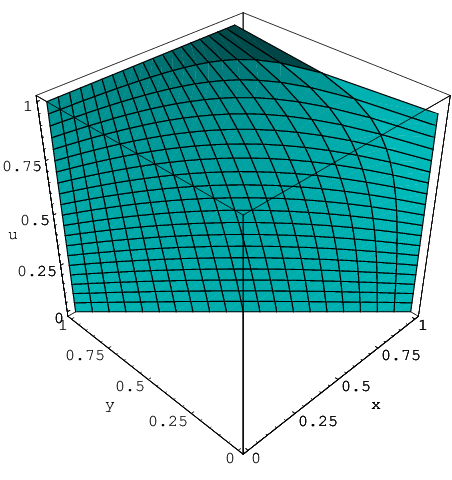
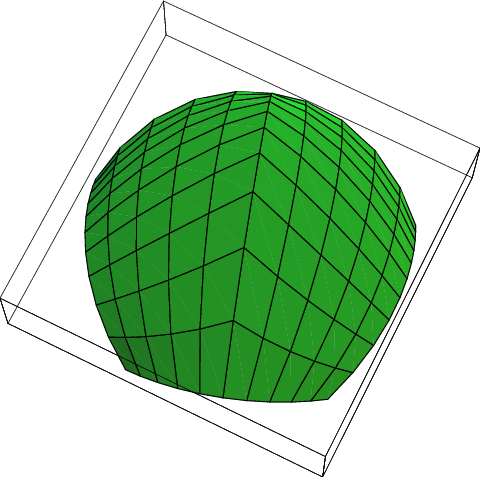
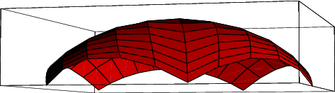
Any pentagon can be represented algebraically by picking two of the five ’s as independent, and plotting any of the dependent variables found by solving the constraints in formula (33) on the third axis. The typical result, shown in Figure 16, is an algebraic 2-manifold embedded in showing the integration region over the variety given by (33). Projected from a horizontal direction, the pentagon of Figure 16(a) becomes a square region, whereas when projected from the vertical direction, it becomes a triangular region,
(a) (b)
(c)
corresponding to formula (2).
To create an image of the twelve components, we now use the constraints (33) and proceed through the same arguments that we used for : We solve the constraints in a family of homogeneous coordinates based on choosing non-singular parameterizations of , and find that the natural connectivity actually gives us initially the 24-pentagon double cover analogous to the six curves shown in Figure 14(a). Figure 17 is the schematic analog of Figure 13 for , showing the topological diagram of the surface, which we can verify is non-orientable with 15 vertices, 30 edges, and 12 pentagonal faces, giving the advertised Euler characteristic , a sphere with five crosscaps. However, we can also see traced on this surface the family of complex lines that form the symmetrized base of the branched cover enabled by the blow-ups: there are 10 separate interlocking triangles, each denoting the (circular) real line of a corresponding precisely to the diagram of Figure 13 or 14(b); treating these schematically as filled-in triangles, we get the image in Figure 18, where the boundaries of the 10 triangles taken five at a time bound the 12 pentagons. The corresponding 12-pentagon figure can be thought of as shown in Figure 17, where the boundaries of the connected components (corresponding to for ) are linear combinations of the ’s. In particular, the face labeled “12” corresponds to a function with a set of exponents that is distinct from the values used in (2), although they are closely related. One can show with suitable variable changes that the exponents corresponding to the primed branch lines (analogous to the exponent at infinity for ) are
| (34) | |||||


The solutions of the constraints are continuous only in the double cover, so we will work first in an unnormalized to produce the analogs of the six end points and six straight interpolating edges that we showed in Figure 14(a) for . This equivalent set of vertices is the set of 10 hexagons representing the double cover of the branch lines denoted by , as shown in Figure 19. These have the following vertex assignments in the double cover:
Each region is bounded by a linear interpolation connecting the (doubled) vertex set, as noted earlier.
Figure 20 shows the actual doubled geometry, both as straight lines in , and as curves in the sphere (projected to 3D).


(a) (b)
Fully Symmetric Vertex Choice.
If all we were interested in was the descriptive topology of the five-crosscap base manifold, any set of vertices with the proper connectivity would be sufficient. However, our dual purpose is to understand not only the topology, but also any unique geometric features or symmetries that might characterize this manifold, leading to embeddings whose graphical depictions might be especially informative.
We have therefore pursued the search for special embeddings one step further, and computed an orthonormalized set of vertices along with the corresponding surface embedding that allows all pentagons to be expressed as rigid transformations of one another derived from the operations of the discrete symmetry operators of Section 4.
The next step is to use the matrix defined by (26). Such a can be found from standard linear algebra methods; we will not write explicitly because its entries are not rational numbers and are very lengthy.
Let
We then get the transformation of the surface . Notice that is in and is invariant under
for ; the ’s are now the orthogonal matrices forming a subgroup of order 240 in .
We pick the following 24 elements from this group:
| (35) |
Then, the entire 5-crosscap surface or its genus-5 double cover can be constructed piece by piece starting from a single pentagon and then transforming by .
In Figure 21, we plot a pair of projections of the 24 surface patches from in to . These are global solutions of the 5-point cross-ratio constraints with diametrically opposite copies of each of the 12 pentagons forming the genus 5 double cover.


Veronese Map.
These vertices and the polygonal faces of the dodecahedron inscribed on the ’s “real” integration manifold, a sphere with five crosscaps, can be compactly embedded for visualization purposes using a quadratic form that is a straightforward generalization of the Veronese surface parameterization. Given the homogeneous variables above, we can construct an embedding as
This map is constructed to lie on the sphere when and the homogeneous coordinates are normalized to obey . Note that the analog of the Steiner Roman Surface immersion projecting into is achieved by selecting the variables mapping into .
An alternative, but less symmetric, embedding is
which also lies on the sphere when .
Projections of the (non-double-covered) 5-crosscap surface can at last be drawn using these quadratic maps, and typical results are shown in Figure 22.


7.4 The Pochhammer Contour
Within the domain of a single pentagon, we can now finally begin to piece together a picture of the global topology of the Pochhammer contour. This manifold can be drawn explicitly in various ways by joining together the sets of commutators that eventually return to the same phase, forming the closed surface; Figure 23 illustrates a single commutator element. Figure 24 shows the schematic diagram of the full set of commutators as they return cyclically to the home phase; this diagram can be unfolded in various ways to show the overall structure, as illustrated in Figures 25 and 26.


(a) (b)
Finally, the explicit algebraic form of the Pochhammer can be embedded directly in the Riemann manifold of , following the fashion of Figure 15 to yield the surfaces shown in Figure 27. This image shows one-fifth of the Pochhammer contour covering a set of eight of the 32 total surfaces; sewing together all the corresponding copies yields the entire surface.
8 Remarks on the General Case
The affine variety defined by the -point cross-ratio constraints (11) is of dimension and has a natural decomposition into smooth components delineated by the varieties . The -point function is initially defined as an integral of an -form over a single one of these components. Each of the components is an -polytope — its -th face is on the projective hyperplane given by ; these are not in general regular polytopes, but reflect the existence of various poles that correspond to multiparticle combinations in elementary spinless string theory. Table 2 summarizes for low the number of cross-ratio variables appearing in the standard constraints, which is also the number of faces of the polytope defining a single component, along with the total number of components. These polytopes have an exact and previously unsuspected correspondence with the Stasheff associahedra [16, 15, 17], in all dimensions. Each of the components, for example, is a nonahedron, as pictured in Figure 28; this structure is described in detail by Devadoss [3], who also gives, for example, a tessellation of the moduli space tiled by 60 nonahedral associahedra. Our work seems to indicate that the moduli spaces studied by Devadoss can also be viewed as the space of -point cross-ratios with the tessellations we have described in this paper.
dim. = no. components 4 2 3 5 5 12 6 9 60 7 14 360 8 20 2520 9 27 20160 10 35 181440

We conjecture that the real integral form of can always be expressed alternatively by a Pochhammer-like contour integral in the corresponding smooth complex algebraic variety of dimension in . The contour is a real -dimensional submanifold and is obtained by wrapping copies of the -polytope integral domain properly around the branch hyperplanes where its faces are located. Notice that it is fairly easy to see, by the description above and (3), that the branch hyperplane at each face – say, face – is of complex codimension 1 in and, when folded around it, the phase of the integrand in the lift to the Riemann covering sheaf changes by . By this mechanism, (6) should generalize in an obvious way.
Acknowledgments
This research was supported in part by NSF grant numbers CCR-0204112 and IIS-0430730. AJH is grateful to Tullio Regge for his early encouragement and interest in this problem. Special thanks are due to Charles Livingston, Philip Chi-Wing Fu, and Sidharth Thakur for advice, insights, and assistance with graphics tools. We also thank James Stasheff for introducing us to the literature on associahedra.
References
- [1] K. Bardakci and H. Ruegg. Reggeized resonance model for the production amplitude. Phys. Letters, 28B:342–347, 1968.
- [2] H. R. Brahana and A. B. Coble. Maps of twelve countries with five sides with a group of order 120 containing an ikosahedral subgroup. Amer. J. Math., 48(1):1–20, 1926.
- [3] Satyan L. Devadoss. Tessellations of moduli spaces and the mosaic operad. In Homotopy invariant algebraic structures. (Baltimore, MD, 1998), volume 239, pages 91–114, Providence, RI, 1999. Amer. Math. Soc.
- [4] T. Goto. Relativistic quantum mechanics of one-dimensional mechanical continuum and subsidiary condition of dual resonance model. Prog. Theor. Phys., 46:457, 1960.
- [5] P. Griffiths and J. Harris. Principles of Algebraic Geometry. Wiley, New York, 1978. (See p. 184.).
- [6] A. J. Hanson. Dual N-point functions in PGL(N-2,C)-invariant formalism. Phys. Rev., D5:1948–1956, 1972.
- [7] D. Hilbert and S. Cohn-Vossen. Geometry and the Imagination. Chelsea, New York, 1952.
- [8] C. Jordan. Cours d’analyse de l’Ecole Polytechnique, volume 3. Gauthier-Villars, Paris, 1887.
- [9] F. Klein. Vorlesungen über das Ikosaeder und die Auflösung der Gleichungen vom fünften Grade. Teubner, Leipzig, 1884. Reprinted Birkhäuser, Basel, 1993 (edited by P. Slodowy); translated as Lectures on the icosahedron and the solution of equations of the fifth degree, Kegan Paul, London, 1913 (2nd edition); reprinted by Dover, 1953.
- [10] Z. Koba and H. B. Nielsen. Manifestly crossing-invariant parameterization of the n-meson amplitude. Nucl. Phys., B12:517–536, 1969.
- [11] Yoichiro Nambu. Duality and hydrodynamics, 1970. Lectures at the Copenhagen High Energy Symposium.
- [12] L.A. Pochhammer. Zur theorie der Euler’schen integrale. Math. Ann., 35:495–526, 1890.
- [13] Joseph Polchinsky. String Theory I. Cambridge University Press, 1998.
- [14] Joseph Polchinsky. String Theory II. Cambridge University Press, 1998.
- [15] James Stasheff. Homotopy associativity of H-spaces. Trans. Amer. Math. Soc., 108:275–292, 1963.
- [16] James Stasheff. H-spaces from a Homotopy Point of View. Lecture Notes in Mathematics 161. Springer Verlag, New York, 1970.
- [17] James Stasheff. What is an operad? Notices Amer. Math. Soc., 51(6):630–631, 2004.
- [18] G. Veneziano. Dual resonance model. Nuovo Cimento, 57A:190, 1968.
- [19] M. A. Virasoro. Generalization of Veneziano’s formula for the five-point function. Phys. Rev. Letters, 22:37–39, 1969.
- [20] M. Weber. Kepler’s small stellated dodecahedron as a Riemann surface. To appear in Pacific Journal of Mathematics, 2005.
- [21] E.T. Whittaker and G.N. Watson. A Course of Modern Analysis. Cambridge University Press, 1969. Republished from the original.