跳到论文正文
W Papers独立论文阅读器 arXiv:math-ph/0510043 论文正文 计算阅读时间 · 0%
引用这篇论文根据当前论文元数据生成,正式投稿前建议核对。


License: Assumed arXiv.org perpetual non-exclusive license
arXiv:math-ph/0510043v2 [math-ph] 12 Oct 2005

Global spectrum fluctuations for the β\beta-Hermite and β\beta-Laguerre ensembles via matrix models

Ioana Dumitriu    Alan Edelman
Abstract

We study the global spectrum fluctuations for β\beta-Hermite and β\beta-Laguerre ensembles via the tridiagonal matrix models introduced in [11], and prove that the fluctuations describe a Gaussian process on monomials. We extend our results to slightly larger classes of random matrices.

1 Introduction

1.1 The Semicircle Law, deviations and fluctuations, numerically

The most celebrated theorem of random matrix theory, the Wigner semicircle law [44, 45], may be illustrated as in Figure 1 by histogramming the eigenvalues of a single random symmetric matrix using the simple MATLAB code (normalization omitted)

𝙰=𝚛𝚊𝚗𝚍𝚗(𝚗);𝚂=(𝙰+𝙰′)/𝚜𝚚𝚛𝚝(𝟾∗𝚗);𝚊=𝚑𝚒𝚜𝚝(𝚎𝚒𝚐(𝚂),[−𝟷:𝚍𝚎𝚕𝚝𝚊:𝟷]);\displaystyle\tt{A=randn(n);~S=(A+A^{\prime})/sqrt(8*n);~a=hist(eig(S),[-1:delta:1]);}
𝚋𝚊𝚛([−𝟷:𝚍𝚎𝚕𝚝𝚊:𝟷],𝚊/(𝚗∗𝚍𝚎𝚕𝚝𝚊))\displaystyle\tt{bar([-1:delta:1],a/(n*delta))}
Refer to caption
Figure 1: 2525 bin-histogram of the eigenvalues of a 300×300300\times 300 symmetric matrix from the real Gaussian distribution, versus the semicircle.

Every time we run this experiment, we obtain deviations from the semicircle. The difference from theory is readily explained computationally:

  • •

    we use a finite matrix size nn, while the semicircle law is a theorem about the n=∞n=\infty limit;

  • •

    histograms bin eigenvalues into boxes of finite width, while the semicircle density is a continuous function.

There can also be numerical error in the experiments due to finite precision computations and truncation error, but in practice this does not appear to be significant.

It is worth noting that the algorithm above is inefficient in two ways: first, it uses the full matrix AA, rather than the equivalent tridiagonal matrix Hβ,nH_{\beta,n} of Table 2 (with β=1\beta=1), and it calculates the eigenvalues to obtain the histogram. For more on how to obtain the histogram plot efficiently and without calculating the eigenvalues, see Section 5.

To study the next order behavior in the law, for large nn, we can subtract away the semicircle and multiply by nn. The next order average behavior is what we call the deviation and it was first computed by Johansson [21] to be

D​E​V​I​A​T​I​O​N=14​δ−1​(x)+14​δ1​(x)−12​π​1−x2.\displaystyle DEVIATION=\frac{1}{4}\delta_{-1}(x)+\frac{1}{4}\delta_{1}(x)-\frac{1}{2\pi}\sqrt{1-x^{2}}~. (1)

This expression for the deviation is the β=1\beta=1 (corresponding to real matrices) instance of the more general β>0\beta>0 case (which was also computed by Johansson, and will be explained in the next sections). The β>0\beta>0 deviation contains a (2β−1)\left(\frac{2}{\beta}-1\right) multiplicative factor in front of the expression on the right of (1), which disappears for β=1\beta=1.

One can see this deviation result as stating that as n→∞n\rightarrow\infty the eigenvalues are decremented in the interior at a rate that is fastest at the center, pulling the eigenvalues toward the endpoints.

Upon further examination of the next-order term, one can observe a phenomenon not appearing in the leading order term; there are fluctuations around the mean.

Each time we run a trial we can compute this fluctuation. For example, if we have 2525 bins, the random fluctuation vector v=(v1,…,v25)Tv=(v_{1},\ldots,v_{25})^{T} is the difference between the count in each bin and the number of eigenvalues predicted by the semicircle plus the deviation. The entries of vv can vary quite wildly, but inner products with discretized smooth functions result in normal distributions in the continuous limit. Specifically, if fkf_{k} is the vector of size 2525 consisting of the evaluations of f⁡(x)=xkf(x)=x^{k} on the centers of the bins, then the dot products fkT​vf_{k}^{T}v are heading towards Gaussians with covariances E⁡[(fk1T​v)​(fk2T​v)]E[(f_{k_{1}}^{T}v)(f_{k_{2}}^{T}v)].

Precise statements require the size of the matrix to go to infinity and the histogram to melt into a smooth density function so that the vv vector becomes a Gaussian process.

Denote by F​L​U​C​T​U​A​T​I​O​N​(f⁡(x))FLUCTUATION(f(x)) the random quantity representing the limit obtained of fT​vf^{T}v where, as above, ff is the vector of function values and vv is the vector of histogram differences. For smooth functions, F​L​U​C​T​U​A​T​I​O​N​(f⁡(x))FLUCTUATION(f(x)) converges to a normal distribution; for example, in the limit as n→∞n\rightarrow\infty,

F​L​U​C​T​U​A​T​I​O​N​(xk)∼2​N​(0,σk2),\displaystyle FLUCTUATION(x^{k})\sim 2N(0,\sigma_{k}^{2})~, (2)

where

σk2={k22​k​(k−1k−12)2,if​k=1mod2,k22​k+2​(kk2)2,if​k=0mod2.\displaystyle\sigma_{k}^{2}=\left\{\begin{array}[]{cl}\frac{k}{2^{2k}}{k-1\choose\frac{k-1}{2}}^{2}~,&\mbox{if}~k=1\mod 2~,\\ \frac{k}{2^{2k+2}}{k\choose\frac{k}{2}}^{2}~,&\mbox{if}~k=0\mod 2~.\end{array}\right.

For general β\beta, the right side of (2) gains a multiplicative factor of 1β\frac{1}{\beta}.

The limit of the entry (k1,k2)(k_{1},k_{2}) of the covariance matrix becomes the covariance between F​L​U​C​T​U​A​T​I​O​N​(xk1)FLUCTUATION(x^{k_{1}}) and F​L​U​C​T​U​A​T​I​O​N​(xk2)FLUCTUATION(x^{k_{2}}) (see Theorem 1.2 with β=1\beta=1).

1.2 β\beta-Hermite and β\beta-Laguerre ensembles

This paper studies deviations and fluctuations in a wider context than real symmetric matrices with semicircular asymptotic density: We consider Hermite and Laguerre matrices with general parameter β>0\beta>0. For a great reference for these ensembles, see Forrester’s upcoming book [16].

Classical finite random matrix theory considers the study of eigenvalue ensembles with joint density

f⁡(x1,…,xn)=cw,n​∏i<j|xi−xj|β​∏i=1nw⁡(xi),f(x_{1},\ldots,x_{n})=c_{w,n}~\prod_{i<j}|x_{i}-x_{j}|^{\beta}\prod_{i=1}^{n}w(x_{i})~,

with ww a scalar weight function on an interval II. This interval may be a subinterval of the real line, or the unit circle in the complex plane; other possibilities have been considered, too, and generalizations are easily conceived. A good reference for these formulae can be found in Mehta’s book [29].

Some of the most studied eigenvalue ensembles have Hermite, Laguerre, and Jacobi weight functions on the real line, or uniform weight on the unit circle. In this paper we will be examining the ensembles with Hermite and Laguerre weights on the real line (respectively, half-line); see Table 1.

Table 1: Random matrix ensembles with eigenvalue distribution proportional to f⁡(x1,…,xn)∝∏i≠j|xi−xj|β​∏w⁡(xi)f(x_{1},\ldots,x_{n})~\varpropto~\prod_{i\neq j}|x_{i}-x_{j}|^{\beta}~\prod w(x_{i}) with ww defined on an interval I⊆ℝI\subseteq\mathbb{R}. MANOVA stands for Multivariate ANalisys Of VAriance.
Name parameters II ww Historical
name/constraints
Hermite 𝜷>𝟎\beta>0 ℝ\mathbb{R} w(x)=e−x2/2w(x)=e^{-x^{2}/2} Gaussian
β=1,2,4\beta=1,2,4
Laguerre 𝜷>𝟎\beta>0 [0,∞)[0,\infty) w(x)=xpe−x/2w(x)=x^{p}e^{-x/2} Wishart
a>(n−1)​β2~a>(n-1)\frac{\beta}{2} p=a−(n−1)​β2−1p=a-(n-1)\frac{\beta}{2}-1 β=1,2\beta=1,2
a=m​β2a=m\frac{\beta}{2}, m∈ℕm\in\mathbb{N}
Jacobi 𝜷>𝟎\beta>0 [0,1][0,1] w⁡(x)=xp1​(1−x)p2w(x)=x^{p_{1}}(1-x)^{p_{2}} MANOVA
a1,a2>(n−1)​β2a_{1},a_{2}>(n-1)\frac{\beta}{2} p1=a1−(n−1)​β2−1p_{1}=a_{1}-(n-1)\frac{\beta}{2}-1 β=1,2\beta=1,2
p2=a2−(n−1)​β2−1p_{2}=a_{2}-(n-1)\frac{\beta}{2}-1 a1=m1​β2a_{1}=m_{1}\frac{\beta}{2}, m1∈ℕm_{1}\in\mathbb{N}
a2=m2​β2a_{2}=m_{2}\frac{\beta}{2}, m2∈ℕm_{2}\in\mathbb{N}

For more references on Gaussian ensembles, see [29]; for Wishart and MANOVA ensembles, see [30]; for Hermite, Laguerre, and Jacobi ensembles, see [16].

For three particular values of β\beta, namely 1,2,1,2, and 44, these ensembles have been studied since the birth of the field, as the Gaussian real, complex, and quaternion ensembles (Hermite with β=1,2,4\beta=1,2,4) of nuclear physics ([44], [45], [14], [1]). Similarly, the Wishart real and complex (Laguerre with β=1,2\beta=1,2 and some restrictions on the Laguerre parameter) matrices emerged from the world of statistical multivariate analysis ([46], [5], [20], [24]).

The parameter β\beta (making the connection to the Boltzmann factor of statistical physics) is seen by some communities (e.g. statistical mechanics) as an inverse temperature, or repulsion strength, of the ensemble of eigenvalues (the higher the β\beta, the more separated the eigenvalues). It also has the advantage of the easy mnemonic of 1,21,2 and 44 corresponding to real, complex, and quaternion entries in the matrix models. However, some communities (like algebraic combinatorics) consider a different parameter, α=2/β\alpha=2/\beta, which tends to simplify certain formulas ([27], [36]). In this paper we will use both notations, for convenience, and make sure that the reader is informed when changes take place.

The reason for the attractivity and success that the study of Gaussian orthogonal, unitary, and symplectic (Hermite with β=1,2,4\beta=1,2,4), and the Wishart real and complex (Laguerre with β=1,2\beta=1,2), ensembles have enjoyed lies in the existence of matrix models with real, complex, and quaternion entries (see [29], [30]). These models have not only originated the study, but have also allowed for a relatively thorough analysis of the finite and asymptotical eigenstatistics (statistical properties of the eigenvalues).

One of the developments in the study of arbitrary β\beta-Hermite, -Laguerre, and -Jacobi ensembles is the introduction of general real matrix models (see [11], [25], [38]). For every β\beta, there are simple real tridiagonal matrices which model the corresponding eigenvalue distributions given by Table 1. For the β\beta-Hermite and -Laguerre ensembles, we present these forms in Table 2. These matrix forms allow for efficient Monte Carlo experiments and an alternative representation for the study of eigenstatistics in the general β\beta case.

This paper contains one example of such analysis. With the help these matrix models, we compute asymptotical global spectrum fluctuations for the β\beta-Hermite and -Laguerre ensembles. For the latter, these results are new in the general β\beta context; the global spectrum fluctuations of complex Wishart matrices (β\beta-Laguerre with β=2\beta=2) were studied by Speicher et al. [26], and before by Cabanal-Duvillard [4]. Johansson’s more extensive study [21] covers our results for the β\beta-Hermite ensembles.

To prove our theorems, we use a very diverse set of methods and techniques from Jack Polynomial theory, special functions, perturbation theory, and combinatorial path-counting. Some of the techniques we used in studying the traces of powers of random matrices have been inspired by the work of Soshnikov and Sinai [33], [34], and by the study of traces of unitary random matrices by Diaconis and Shahshahani [9].

Table 2: Unscaled and scaled tridiagonal matrix models for the β\beta-Hermite and β\beta-Laguerre ensembles with any β>0\beta>0, n∈ℕn\in\mathbb{N}, a∈ℝa\in\mathbb{R}, and a>β2​(n−1)a>\frac{\beta}{2}(n-1).
Hermite matrix,unscaled\begin{array}[]{c}\mbox{{Hermite} matrix,}\\ \textbf{unscaled}\end{array} Hβ,nH_{\beta,n} ∼12​(N⁡(0,2)χ(n−1)​βχ(n−1)​βN⁡(0,2)χ(n−2)​β⋱⋱⋱χ2​βN⁡(0,2)χβχβN⁡(0,2))\sim\frac{1}{\sqrt{2}}\left(\begin{array}[]{ccccc}N(0,2)&\chi_{(n-1)\beta}&&&\\ \chi_{(n-1)\beta}&N(0,2)&\chi_{(n-2)\beta}&&\\ &\ddots&\ddots&\ddots&\\ &&\chi_{2\beta}&N(0,2)&\chi_{\beta}\\ &&&\chi_{\beta}&N(0,2)\end{array}\right)
Hermite matrix,scaled\begin{array}[]{c}\mbox{{Hermite} matrix,}\\ \textbf{scaled}\end{array} H~β,n=12​n​β​Hβ,n\tilde{H}_{\beta,n}~=~\frac{1}{\sqrt{2n\beta}}~H_{\beta,n}
Laguerre matrix,unscaled\begin{array}[]{c}\mbox{{Laguerre} matrix,}\\ \textbf{unscaled}\end{array} Lβ,naL_{\beta,n}^{a} =Bβ,na​(Bβ,na)T=B_{\beta,n}^{a}(B_{\beta,n}^{a})^{T}, where
     Bβ,na∼(χ2​aχβ⁡(n−1)χ2​a−β⋱⋱χβχ2​a−β⁡(n−1))B_{\beta,n}^{a}\sim\left(\begin{array}[]{cccc}\chi_{2a}&&&\\ \chi_{\beta(n-1)}&\chi_{2a-\beta}&&\\ &\ddots&\ddots&\\ &&\chi_{\beta}&\chi_{2a-\beta(n-1)}\end{array}\right)
Laguerre matrix,scaled\begin{array}[]{c}\mbox{{Laguerre} matrix,}\\ \textbf{scaled}\end{array} L~β,na=γn​β​Lβ,na\tilde{L}_{\beta,n}^{a}~=~\frac{\gamma}{n\beta}~L_{\beta,n}^{a}

1.3 Statements of results

Among the asymptotical eigenstatistics one may distinguish two classes of properties: local (like the scaled distributions and fluctuations of extremal eigenvalues, or like the level spacing distribution, i.e., the distance between neighboring eigenvalues) and global (like the limiting level density, i.e. the distribution of a random eigenvalue, and fluctuations thereof). The term global tends to refer to a property that involves all or a significant portion of the eigenvalues, while local tends to refer to a property that occurs near an individual or a constant number of eigenvalues. Among the more famous local properties we enumerate the level spacings for the Gaussian ensembles (see [29], [39]) and the extremal (largest, corresponding to “soft edge”, smallest, to “hard edge”) eigenvalue asymptotics (see [41], [40], [22], [23]). All these results relate to real, complex, or quaternion matrices; in the category of results relating to general β\beta, we have to mention recent work by Desrosiers and Forrester [8], where they analyze the asymptotical corrections to the eigenvalue density, and, for β∈2​ℕ\beta\in 2\mathbb{N}, obtain the expected O⁡(n2/3)O(n^{2/3}) order in the fluctuation of the largest eigenvalue in the case of both β\beta-Hermite and -Laguerre ensembles.

For nn (the size of the ensembles) finite, the nn eigenvalues may be considered as nn fluctuating particles. Roughly speaking, the larger the β\beta, the less fluctuation there is in the particles (hence β\beta is seen as an inverse temperature). As β→∞\beta\rightarrow\infty the particle positions behave like multivariate normals with variance O⁡(1/β)O(1/\beta) and means located at the roots of a Hermite (respectively Laguerre) polynomial (see [12]).

For a fixed β\beta, as n→∞n\rightarrow\infty and, in the case of Laguerre ensembles, 2​a/(n​β)→γ2a/(n\beta)\rightarrow\gamma, the particles have an emerging (global) level density which is obeys a simple law (Wigner’s semicircle law [45] for the Hermite ensembles, Marčenko-Pastur laws [28] for the Laguerre ensembles). The roots of the Hermite, respectively Laguerre, polynomial have this same asymptotical density – the fluctuations do not change the asymptotics, as they are on a smaller scale.

In [10], we have proved convergence almost surely (as n→∞n\rightarrow\infty) of the asymptotical eigenvalue distribution of the β\beta-Hermite ensemble to the semicircle distribution SS with density 2π​1−x2\frac{2}{\pi}\sqrt{1-x^{2}}, and of the asymptotical eigenvalue distribution of the β,a\beta,a-Laguerre ensemble (with n​β/(2​a)→γ≤1n\beta/(2a)\rightarrow\gamma\leq 1) to the Marčenko-Pastur EγE_{\gamma} distribution with density 12​π​γ​(x−(γ−1)2)​((γ+1)2−x)x\frac{1}{2\pi\gamma}\frac{\sqrt{(x-(\sqrt{\gamma}-1)^{2})((\sqrt{\gamma}+1)^{2}-x)}}{x}. We recall that convergence almost surely is stronger (and implies) convergence in distribution, a.k.a. convergence of moments.

We examine here the distribution of the statistic ∑i=1nf⁡(λi)\sum\limits_{i=1}^{n}f(\lambda_{i}), where ff is a function of the scaled eigenvalues λi\lambda_{i}. The scaling is λ→2​n​β​λ\lambda\rightarrow\sqrt{2n\beta}\lambda for the β\beta-Hermite ensembles and λ→n​β/γ​λ\lambda\rightarrow n\beta/\gamma\lambda for the β\beta-Laguerre ensembles (see Table 2).

General β\beta results for this kind of statistic can be found in [6], [21]; this or similar linear statistics have been considered also in [15] (for unitary matrices), [32] (for Wishart matrices), and, heuristically, in [31]. Another path of interest is represented by asymptotical large deviations from the density (spectral measure); we mention the results of [4], [2], [18] (which also covers global fluctuations for Wishart matrices) , [19], [7] (which covers moderate deviations).

For the linear statistic ∑i=1nf⁡(λi)\sum_{i=1}^{n}f(\lambda_{i}), the Wigner and Marčenko-Pastur laws for the β\beta-Hermite and β\beta-Laguerre ensembles state that for any “well-behaved” function ff,

1n​∑i=1nf⁡(λi)\displaystyle\frac{1}{n}~\sum_{i=1}^{n}f(\lambda_{i}) →\displaystyle\rightarrow 2π​∫−11f⁡(t)​1−t2​𝑑t,respectively,\displaystyle\frac{2}{\pi}\int_{-1}^{1}f(t)\sqrt{1-t^{2}}~dt~,~\mbox{respectively,} (4)
1n​∑i=1nf⁡(λi)\displaystyle\frac{1}{n}~\sum_{i=1}^{n}f(\lambda_{i}) →\displaystyle\rightarrow 12​π​γ​∫(γ−1)2(γ+1)2f⁡(t)​(t−(γ−1)2)​((γ+1)2−t)t​𝑑t,\displaystyle\frac{1}{2\pi\gamma}\int_{(\sqrt{\gamma}-1)^{2}}^{(\sqrt{\gamma}+1)^{2}}f(t)~\frac{\sqrt{(t-(\sqrt{\gamma}-1)^{2})((\sqrt{\gamma}+1)^{2}-t)}}{t}~dt~, (5)

where the convergence in the above is almost surely11 1 Such a result is sometimes given the name of “Strong Law of Large Numbers”; if convergence is only in distribution, the name becomes “Law of Large Numbers”..

Examining the fluctuations from these laws takes us one step further. For ff a polynomial, we prove that once we subtract the expected average over the limiting level density (i.e. the right hand sides of (4) and (5)), the rescaled resulting quantity tends asymptotically to a normal distribution with mean and variance depending on ff. In other words, once the semicircle or Marčenko-Pastur distributions are subtracted, the fluctuations in the statistic ∑i=1nf⁡(λi)\sum\limits_{i=1}^{n}f(\lambda_{i}) tend asymptotically to a Gaussian process on polynomials ff.

How much more we can extend the class of functions that this process is well-defined on depends on the entries of the covariance matrix C={Ci​j}C=\{C_{ij}\} (which can be expressed in any polynomial basis). One would be tempted to believe that a Gaussian process WW defined on polynomials could, in principle, be extended to a class of continuous functions h⁡(x)h(x) with the property that, given a sequence of polynomials pn​(x)→h​(x)p_{n}(x)\rightarrow h(x) in some norm, given vn=V​a​rW​(pn)v_{n}=Var_{W}(p_{n}), vn→v~<∞v_{n}\rightarrow\tilde{v}<\infty, such that v~=V​a​rW​(h)\tilde{v}=Var_{W}(h).

Definition 1.1.

Let γ∈[0,1]\gamma\in[0,1] be a real parameter, and let a=(γ−1)2a=(\sqrt{\gamma}-1)^{2}, b=(γ+1)2b=(\sqrt{\gamma}+1)^{2}. We define the following two measures:

μH​(x)\displaystyle\mu_{H}(x) :⁣=\displaystyle:= {14​δ1​(x)+14​δ−1​(x)−12​π​11−x2,if x∈[−1,1],0,otherwise.,\displaystyle\left\{\begin{array}[]{cl}\frac{1}{4}\delta_{1}(x)+\frac{1}{4}\delta_{-1}(x)-\frac{1}{2\pi}\frac{1}{\sqrt{1-x^{2}}},&\mbox{if $x\in[-1,1]$}~,\\ 0~,&\mbox{otherwise.}\end{array}\right.~,
μLγ​(x)\displaystyle\mu_{L}^{\gamma}(x) :⁣=\displaystyle:= {14​δb​(x)+14​δa​(x)−12​π​1(x−a)​(b−x),if x∈[a,b],0,otherwise .\displaystyle\left\{\begin{array}[]{cl}\frac{1}{4}\delta_{b}(x)+\frac{1}{4}\delta_{a}(x)-\frac{1}{2\pi}\frac{1}{\sqrt{(x-a)(b-x)}}~,&\mbox{if $x\in[a,b]$}~,\\ 0~,&\mbox{otherwise~.}\end{array}\right.
Theorem 1.2.

Let H~β,n\tilde{H}_{\beta,n} be a scaled matrix from the β\beta-Hermite ensemble of size nn, with (scaled) eigenvalues (λ1,…,λn)(\lambda_{1},\ldots,\lambda_{n}), and let k≥1k\geq 1 be a positive integer. For all i=1,…,ki=1,\ldots,k, let

Xi\displaystyle X_{i} =\displaystyle= t​r​((H~β,n)i)−n​14i/2​(i2+1)​(ii2)​δ(imod2),0−(2β−1)​∫−11ti​μH​(t)​𝑑t,\displaystyle tr((\tilde{H}_{\beta,n})^{i})-n~\frac{1}{4^{i/2}\left(\frac{i}{2}+1\right)}{i\choose\frac{i}{2}}\delta_{(i\!\!\!\!\mod 2),0}-\left(\frac{2}{\beta}-1\right)\int_{-1}^{1}t^{i}\mu_{H}(t)~dt,
≡\displaystyle\equiv ∑j=1nλji−n​2π​∫−11ti​1−t2​𝑑t−(2β−1)​∫−11ti​μH​(t)​𝑑t.\displaystyle\sum_{j=1}^{n}\lambda_{j}^{i}~-~n~\frac{2}{\pi}\int_{-1}^{1}t^{i}\sqrt{1-t^{2}}~dt~-~\left(\frac{2}{\beta}-1\right)\int_{-1}^{1}t^{i}\mu_{H}(t)~dt~~.

Let (Y1,Y2,…,Yk)(Y_{1},Y_{2},\ldots,Y_{k}) be a centered multivariate Gaussian with covariance matrix

Cov​(Yi,Yj)={12i+j​2​i​ji+j​(i−1i−12)​(j−1j−12),if​i=j=1mod2;12i+j+2​2​i​ji+j​(ii2)​(jj2),if​i=j=0mod2;0,otherwise.\displaystyle\mbox{Cov}(Y_{i},Y_{j})=\left\{\begin{array}[]{ll}\frac{1}{2^{i+j}}\frac{2ij}{i+j}{i-1\choose\frac{i-1}{2}}{j-1\choose\frac{j-1}{2}}~,&\mbox{if}~~i=j=1\mod 2~;\\ \frac{1}{2^{i+j+2}}\frac{2ij}{i+j}{i\choose\frac{i}{2}}{j\choose\frac{j}{2}}~,&\mbox{if}~~i=j=0\mod 2~;\\ 0~,&\mbox{otherwise.}\end{array}\right.

Then, as n→∞n\rightarrow\infty,

(X1,X2,…,Xk)⇒2β​(Y1,Y2,…,Yk).(X_{1},X_{2},\ldots,X_{k})\Rightarrow\sqrt{\frac{2}{\beta}}~(Y_{1},Y_{2},\ldots,Y_{k})~.
Remark 1.3.

For any size kk, if we add a first row and a first column of zeros to the covariance matrix (1.2), the resulting (k+1)×(k+1)(k+1)\times(k+1) matrix CkC_{k} has a scaled Cholesky decomposition as Ck=Tk​Dk​TkTC_{k}=T_{k}D_{k}T_{k}^{T}, where DkD_{k} is the diagonal matrix having on the diagonal the vector (0,1,2,3,…,k)(0,1,2,3,\ldots,k), and TkT_{k} has an interpretation as the change-of-base matrix in the space of univariate polynomials from monomials basis to the Chebyshev polynomials basis. One can also look at the infinite version C∞=T∞​D∞​T∞TC_{\infty}=T_{\infty}D_{\infty}T_{\infty}^{T}.

Remark 1.4.

This Gaussian process is extended to a larger class of continuous functions in [21]. Johansson conjectured that the regularity conditions imposed were purely technical, and that in fact the correct condition should be that the function hh admits a Fourier-like expansion in the Chebyshev basis, which we write as an (infinite) vector h→\vec{h}, such that h→T​D∞​h→\vec{h}^{T}D_{\infty}\vec{h}, the variance of hh under the process, is finite. This conjecture is equivalent to saying that the process could be extended to any function ff such that f→T​C∞​f→\vec{f}^{T}C_{\infty}\vec{f} is finite (since we have chosen the monomial basis as the representation, rather than the Chebyshev polynomial basis).

Theorem 1.5.

Let L~β,na\tilde{L}_{\beta,n}^{a} be a scaled matrix from the β\beta-Laguerre ensemble of parameter aa and size nn, with (scaled) eigenvalues (λ1,…,λn)(\lambda_{1},\ldots,\lambda_{n}), and let k≥1k\geq 1 be a positive integer. Assume that n​β/(2​a)→γ≤1n\beta/(2a)\rightarrow\gamma\leq 1, and let γm​i​n=(γ−1)2,γm​a​x=(γ+1)2\gamma_{min}=(\sqrt{\gamma}-1)^{2},~\gamma_{max}=(\sqrt{\gamma}+1)^{2}. For all i=1,…,ki=1,\ldots,k, let

Xi\displaystyle X_{i} =\displaystyle= t​r​((L~β,na)i)−n​∑r=0i−11r+1​(kr)​(k−1r)​γr−(2β−1)​∫γm​i​nγm​a​xti​μLγ​(t)​𝑑t,\displaystyle tr((\tilde{L}^{a}_{\beta,n})^{i})-n~\sum_{r=0}^{i-1}\frac{1}{r+1}{k\choose r}{k-1\choose r}\gamma^{r}-\left(\frac{2}{\beta}-1\right)\int_{\gamma_{min}}^{\gamma_{max}}\!\!t^{i}\mu_{L}^{\gamma}(t)~dt,
≡\displaystyle\equiv ∑j=1nλji−n​12​π​γ​∫γm​i​nγm​a​xti​(t−γm​i​n)​(γm​a​x−t)​𝑑t−(2β−1)​∫γm​i​nγm​a​xti​μLγ​(t)​𝑑t.\displaystyle\sum_{j=1}^{n}\lambda_{j}^{i}~-~n~\frac{1}{2\pi\gamma}\int_{\gamma_{min}}^{\gamma_{max}}\!\!t^{i}\sqrt{(t-\gamma_{min})(\gamma_{max}-t)}~dt~-~\left(\frac{2}{\beta}-1\right)\int_{\gamma_{min}}^{\gamma_{max}}\!\!t^{i}\mu_{L}^{\gamma}(t)~dt~~.

Let (Y1,Y2,…,Yk)(Y_{1},Y_{2},\ldots,Y_{k}) be a centered multivariate Gaussian with covariance matrix

Cov​(Yi,Yj)=TD​(i,j)+TS​(i,j),\displaystyle\mbox{Cov}(Y_{i},Y_{j})=T_{D}(i,j)+T_{S}(i,j)~, (12)

where

TD​(i,j)=∑q=1i+j−1(−1)q+1​γi+j−q​(i+jq)i+j​∑l=q+1i+j(−1)l(i+j−1l−1)​∑r+s=l1≤r≤i1≤s≤jr​s​(ir)2​(js)2,T_{D}(i,j)=\sum_{q=1}^{i+j-1}(-1)^{q+1}\gamma^{i+j-q}\frac{{i+j\choose q}}{i+j}\sum_{l=q+1}^{i+j}\frac{(-1)^{l}}{{i+j-1\choose l-1}}\sum_{\begin{array}[]{c}r+s=l\\ 1\leq r\leq i\\ 1\leq s\leq j\end{array}}rs{i\choose r}^{2}{j\choose s}^{2}~,

and

TS​(i,j)=∑q=0i+j−2(−1)q​γi+j−q​(i+jq)i+j​∑l=qi+j−2(−1)l(i+j−1l)​∑r+s=l0≤r≤i−10≤s≤j−1(i−r)​(j−s)​(ir)2​(js)2.T_{S}(i,j)=\sum_{q=0}^{i+j-2}(-1)^{q}\gamma^{i+j-q}\frac{{i+j\choose q}}{i+j}\sum_{l=q}^{i+j-2}\frac{(-1)^{l}}{{i+j-1\choose l}}\sum_{\begin{array}[]{c}r+s=l\\ 0\leq r\leq i-1\\ 0\leq s\leq j-1\end{array}}(i-r)(j-s){i\choose r}^{2}{j\choose s}^{2}~.

Then, as n→∞n\rightarrow\infty,

(X1,X2,…,Xk)⇒2β​(Y1,Y2,…,Yk).(X_{1},X_{2},\ldots,X_{k})\Rightarrow\sqrt{\frac{2}{\beta}}~(Y_{1},Y_{2},\ldots,Y_{k})~.
Remark 1.6.

For any size kk, if we add a first row and a first column of zeros to the covariance matrix (12), the resulting matrix CC should admit a scaled Cholesky decomposition of the form Ck=Tk​Dk​TkTC_{k}=T_{k}D_{k}T_{k}^{T}, with DkD_{k} being the diagonal matrix with diagonal entries {j​γ−j}0≤j≤k\{j\gamma^{-j}\}_{0\leq j\leq k}, and TkT_{k} being the change-of-basis matrix in the space of polynomials from monomial basis to the shifted Chebyshev polynomials of the first kind (as defined by Cabanal-Duvillard [4] and used in [26]). Note that the constant cc in [26] is our 1/γ1/\gamma. It may also be useful to look at C∞=T∞​D∞​T∞TC_{\infty}=T_{\infty}D_{\infty}T_{\infty}^{T}.

Remark 1.7.

It is worth noting that results like Theorems 1.2 and 1.5, where one averages over a set of quantities, then subtracts the mean and scales by the variance to obtain a limiting Gaussian, are sometimes called central limit theorems (see for example [32] and [33]). Free Probability uses this term as well, see for example [35], in a different context, namely, to express the fact that averaging over random matrices creates an eigenvalue distribution that approaches the semi-circular law. Both uses of the term “central limit theorem” draw different parallels to the classical case.

Our approach to proving Theorems 1.2 and 1.5 consists of computing the first-order deviation from the mean (in Section 2), showing that the centered process is Gaussian on monomials (by the method of moments), and computing the covariance matrices (in Section 3).

Finally, in Section 4, we generalize our approach to two different classes of random matrices.

2 Deviation from the semicircle and Marčenko-Pastur laws

2.1 Dependence on β\beta: symmetric functions and the “palindrome” effect

As stated in the introduction, we are interested in computing the deviation to the semicircle and Marčenko-Pastur laws (denoted below by L​A​W​(∞)LAW(\infty), as opposed to the L​A​W​(n)LAW(n), which is the level density for finite nn). These deviations have the form

L​A​W​(n)∼L​A​W​(∞)+1n​(1−2β)​D​E​V​I​A​T​I​O​N​(β=∞)+o⁡(1n),LAW(n)\sim LAW(\infty)+\frac{1}{n}\left(1-\frac{2}{\beta}\right)DEVIATION(\beta=\infty)+o\left(\frac{1}{n}\right)~,

as n→∞n\rightarrow\infty.

By integrating the above against xkx^{k}, we can write this in the moment form

m​o​m​e​n​tk​(n)=m​o​m​e​n​tk​(∞)+1n​(1−2β)​m​o​m​e​n​tk​(D​E​V​I​A​T​I​O​N​(β=∞))+o⁡(1n),moment_{k}(n)=moment_{k}(\infty)+\frac{1}{n}\left(1-\frac{2}{\beta}\right)moment_{k}(DEVIATION(\beta=\infty))+o\left(\frac{1}{n}\right)~,

again as n→∞n\rightarrow\infty.

We mention two interesting points, the first of which we prove in this section:

  1. 1.

    The factor 2β−1\frac{2}{\beta}-1 can be obtained from a symmetry principle alone. It is a direct consequence of Jack Polynomial theory that the coefficient of 1/nj1/n^{j} in m​o​m​e​n​tk​(n)moment_{k}(n) is a palindromic polynomial (we define “palindromic” below) in −2β-\frac{2}{\beta}, and from the tridiagonal matrix models it follows that the degree of this polynomial is jj; thus when j=1j=1 this polynomial must be a multiple of 2β−1\frac{2}{\beta}-1. Mathematically, this is significant because because in order to study the deviations, it is sufficient to then study the non-random case, β=∞\beta=\infty. In summary, the powerful Jack Polynomial theory allows us to take a complicated random matrix problem and reduce it to an exercise on the properties of univariate Hermite and Laguerre polynomials.

  2. 2.

    With the Maple Library MOPs [13], we can compute symbolically the exact values of m​o​m​e​n​tk​(n)moment_{k}(n) for small values of kk, as a function of nn and β\beta. In other words, while this paper concerns itself with the constant and O⁡(1/n)O(1/n) behavior, it is worth remembering that higher order terms are in principle available to us.

To make notation a bit clearer, we have used the α=2/β\alpha=2/\beta in the below; we also recall the scaled matrices H~β,n\tilde{H}_{\beta,n} and L~β,na\tilde{L}_{\beta,n}^{a}, from Section 1.2. The following are the first three non-trivial moments for the traces of the scaled β\beta-Hermite and β\beta-Laguerre matrices with a=n​β/(2​γ)=n/(α​γ)a=n\beta/(2\gamma)=n/(\alpha\gamma). We omit the nn and aa in the notation for reasons of space.

1n​E​[tr​(H2/α2)]\displaystyle\!\!\!\!\frac{1}{n}~E[\mbox{tr}(H_{2/\alpha}^{2})] =\displaystyle= 14+α−14​n,\displaystyle\frac{1}{4}+\frac{\alpha-1}{4n},~
1n​E​[tr​(H2/α4)]\displaystyle\!\!\!\!\frac{1}{n}~E[\mbox{tr}(H_{2/\alpha}^{4})] =\displaystyle= 216+5​α−516​n+3​α2−5​α+316​n2,\displaystyle\frac{2}{16}+\frac{5\alpha-5}{16n}+\frac{3\alpha^{2}-5\alpha+3}{16n^{2}},~
1n​E​[tr​(H2/α6)]\displaystyle\!\!\!\!\frac{1}{n}~E[\mbox{tr}(H_{2/\alpha}^{6})] =\displaystyle= 564+11​α−1132​n+16​α2−27​α+1632​n2+15​α3−32​α2+32​α−1564​n3,\displaystyle\frac{5}{64}+\frac{11\alpha-11}{32n}+\frac{16\alpha^{2}-27\alpha+16}{32n^{2}}+\frac{15\alpha^{3}-32\alpha^{2}+32\alpha-15}{64n^{3}},~
1n​E​[tr​(L2/α)]\displaystyle\!\!\!\!\frac{1}{n}~E[\mbox{tr}(L_{2/\alpha})] =\displaystyle= 1,\displaystyle 1~,
1n​E​[tr​(L2/α2)]\displaystyle\frac{1}{n}~E[\mbox{tr}(L_{2/\alpha}^{2})] =\displaystyle= (1+γ)+γ⁡(α−1)n,\displaystyle(1+\gamma)+\frac{\gamma(\alpha-1)}{n}~,
1n​E​[tr​(L2/α3)]\displaystyle\frac{1}{n}~E[\mbox{tr}(L_{2/\alpha}^{3})] =\displaystyle= (1+3​γ+γ2)+3​γ​(γ+1)​(α−1)n+γ2​(2​α2−3​α+2)n2.\displaystyle(1+3\gamma+\gamma^{2})+\frac{3\gamma(\gamma+1)(\alpha-1)}{n}+\frac{\gamma^{2}(2\alpha^{2}-3\alpha+2)}{n^{2}}~.

Note that the O⁡(1)O(1) terms in the above correspond to the second, fourth, and sixth moments of the semicircle, in the Hermite case, respectively, to the first, second, and third moments of the Marčenko-Pastur distributions in the Laguerre case; these are Catalan numbers (scaled down by powers of 44 because of the semicircle [−1,1][-1,1] normalization), respectively Narayana polynomials in γ\gamma.

The O⁡(1/n)O(1/n) terms, the moments of the deviation, are always multiplied by α−1\alpha-1, while the other coefficients of the negative powers of nn in the above are “palindromic polynomials” of (−α)(-\alpha); we recall the definition below.

Definition 2.1.

A classical “palindromic polynomial” is defined by the fact that its list of coefficients, is the same whether read from beginning to end or from end to beginning.

Remark 2.2.

An odd-degree palindromic polynomial in xx is a multiple of (x+1)(x+1).

To prove that the dependence of the first-order term in the deviation is indeed a multiple of α−1\alpha-1, i.e., of 2β−1\frac{2}{\beta}-1, we will use elements of Jack polynomial theory, and also a stronger form of a duality principle proved in [10].

We introduce below two notational conventions to be used throughout the rest of the paper.

Definition 2.3.

We denote by EδH​[P⁡(x1,…,xs)]E_{\delta}^{H}[P(x_{1},\ldots,x_{s})], respectively Eδ,aL​[P⁡(x1,…,xs)]E_{\delta,a}^{L}[P(x_{1},\ldots,x_{s})], the expectations of the polynomial PP over the scaled 2/δ2/\delta-Hermite, respectively 2/δ,a2/\delta,a-Laguerre, ensembles of size ss.

We denote by ℰδH​[P⁡(x1,…,xs)]\mathcal{E}_{\delta}^{H}[P(x_{1},\ldots,x_{s})], respectively ℰδ,aL​[P⁡(x1,…,xs)]\mathcal{E}_{\delta,a}^{L}[P(x_{1},\ldots,x_{s})], the expectations of the polynomial PP over the unscaled 2/δ2/\delta-Hermite, respectively 2/δ,a2/\delta,a-Laguerre, ensembles of size ss.

Let ℝ⁡[x1,…,xn]\mathbb{R}[x_{1},\ldots,x_{n}] be the space of symmetric polynomials in nn variables (by symmetric we mean invariant under any permutation of the variables). A homogeneous basis for this vector space is a set of linearly independent, symmetric and homogeneous polynomials which generate ℝ⁡[x1,…,xn]\mathbb{R}[x_{1},\ldots,x_{n}]. One such basis is given by the power-sum functions, defined multiplicatively below. For reference, see [37] and [27].

Definition 2.4.

Let λ≡(λ1,λ2,…,λn)\lambda\equiv(\lambda_{1},\lambda_{2},\ldots,\lambda_{n}) denote an ordered partition (λ1≥λ2≥…≥λn𝐶𝐿𝑂𝑆𝐸(\lambda_{1}\!\geq\!\lambda_{2}\!\geq\!\ldots\!\geq\!\lambda_{n}). We define the power sum functions by

pλi\displaystyle p_{\lambda_{i}} =\displaystyle= ∑j=1nxjλi,and\displaystyle\sum_{j=1}^{n}x_{j}^{\lambda_{i}}~,~~~~\mbox{and}
pλ\displaystyle p_{\lambda} =\displaystyle= pλ1​pλ2​…​pλn.\displaystyle p_{\lambda_{1}}p_{\lambda_{2}}\ldots p_{\lambda_{n}}~.

The Jack polynomials JλαJ_{\lambda}^{\alpha} constitute a parameter-dependent (the parameter being usually denoted by α\alpha) class of orthogonal multivariate polynomials; they are indexed by the powers of the highest-order term λ\lambda (in lexicographical ordering).

Throughout this section, we will think of the parameter α\alpha as a sort of inverse to β\beta (recall that we have denoted α=2/β\alpha=2/\beta).

The Jack polynomials allow for several equivalent definitions (up to certain normalization constraints). We will work here with definition 2.5, which arose in combinatorics. We follow Macdonald’s book [27].

Definition 2.5.

The Jack polynomials JλαJ_{\lambda}^{\alpha} are orthogonal with respect to the inner product defined below on power-sum functions

⟨pλ,pμ⟩α=αl⁡(λ)​zλ​δλ​μ,\langle p_{\lambda},p_{\mu}\rangle_{\alpha}=\alpha^{l(\lambda)}z_{\lambda}\delta_{\lambda\mu},

where zλ=∏i=1l⁡(λ)ai!​iaiz_{\lambda}=\prod\limits_{i=1}^{l(\lambda)}a_{i}!i^{a_{i}}, aia_{i} being the number of occurrences of ii in λ\lambda. In addition, the coefficient of the lowest-order term in JλαJ_{\lambda}^{\alpha}, which corresponds to the partition [1|λ|]≡(1,1,…,1)[1^{|\lambda|}]\equiv(1,1,\ldots,1) (of length |λ||\lambda|), is |λ|!|\lambda|!.

From now on, we will use the notations InI_{n} for the vector of nn ones and we will refer to the quantity Jκα​(x1,…,xn)/Jκα​(In)J_{\kappa}^{\alpha}(x_{1},\ldots,x_{n})/J_{\kappa}^{\alpha}(I_{n}) as the normalized Jack polynomial.

To prove our results, we will need the two lemmas below, the first of which is a stronger variant of the duality principle proved in [10] as Theorem 8.5.3 (the proof is virtually the same as in [10] and we will not repeat it here). The second one is a rewrite of a particular case (za=0z_{a}=0 and formula (4.14a)) of formula (4.36b) in [3].

Lemma 2.6.

Let κ′\kappa^{\prime} denote the conjugate partition to κ\kappa (obtained by transposing the rows and columns in the Young tableau). Then the following is true:

ℰαH[Jκα​(x1,…,xn)Jκα​(In)]=(−α)−k/2ℰ1/αH[Jκ′1/α​(y1,…,ym)Jκ′1/α​(Im)].\displaystyle\mathcal{E}_{\alpha}^{H}\left[\frac{J_{\kappa}^{\alpha}(x_{1},\ldots,x_{n})}{J_{\kappa}^{\alpha}(I_{n})}\right]=(-\alpha)^{-k/2}\mathcal{E}_{1/\alpha}^{H}\left[\frac{J_{\kappa^{\prime}}^{1/\alpha}(y_{1},\ldots,y_{m})}{J_{\kappa^{\prime}}^{1/\alpha}(I_{m})}\right]~.
Lemma 2.7.

The following identity is true:

ℰα,aL​[Jκα​(x1,…,xn)Jκα​(In)]=∏(x,y)∈κ(a−xα+y).\displaystyle\mathcal{E}_{\alpha,a}^{L}\left[\frac{J_{\kappa}^{\alpha}(x_{1},\ldots,x_{n})}{J_{\kappa}^{\alpha}(I_{n})}\right]=\prod_{(x,y)\in\kappa}\left(a-\frac{x}{\alpha}+y\right)~.

In particular, for a=nα​γa=\frac{n}{\alpha\gamma},

ℰα,nγ​αL​[Jκα​(x1,…,xn)Jκα​(In)]=∏(x,y)∈κ(nα​γ−xα+y).\displaystyle\mathcal{E}_{\alpha,\frac{n}{\gamma\alpha}}^{L}\left[\frac{J_{\kappa}^{\alpha}(x_{1},\ldots,x_{n})}{J_{\kappa}^{\alpha}(I_{n})}\right]=\prod_{(x,y)\in\kappa}\left(\frac{n}{\alpha\gamma}-\frac{x}{\alpha}+y\right)~.

We can now prove the two main results of this section.

Theorem 2.8.

For kk an even integer, let

ℰαH​[p[k]​(x1,…,xn)]=∑j=0k2f⁡(α,j)​nk2+1−j,\displaystyle\mathcal{E}_{\alpha}^{H}\left[p_{[k]}(x_{1},\ldots,x_{n})\right]=\sum_{j=0}^{\frac{k}{2}}f(\alpha,j)~n^{\frac{k}{2}+1-j}~,

with p[k]p_{[k]} being the power-sum corresponding to partition [k][k]. Then f⁡(α,j)f(\alpha,j) is an integer-coefficient polynomial in 1/α1/\alpha of degree at most k/2k/2 such that

f⁡(α,j)=(−α)−k+j​f​(1/α,j).f(\alpha,j)=(-\alpha)^{-k+j}f(1/\alpha,j)~.
Remark 2.9.

When we scale the ensembles, we have to multiply the expectation by (2nβ)−k/2=(α4​n)k/2(2n\beta)^{-k/2}=\left(\frac{\alpha}{4n}\right)^{k/2}, which means that

1n​EαH​[p[k]​(x1,…,xn)]=14k/2​∑j=0k2αk/2​f​(α,j)​n−j.\displaystyle\frac{1}{n}E_{\alpha}^{H}\left[p_{[k]}(x_{1},\ldots,x_{n})\right]=\frac{1}{4^{k/2}}\sum_{j=0}^{\frac{k}{2}}\alpha^{k/2}f(\alpha,j)~n^{-j}~.

The corollary below follows.

Corollary 2.10.

It follows that g⁡(α,j):=αk/2​f​(α,j)g(\alpha,j):=\alpha^{k/2}f(\alpha,j) is an integer-coefficient polynomial of α\alpha for which

g⁡(α,j)=(−α)j​g​(1α,j),g(\alpha,j)=(-\alpha)^{j}g(\frac{1}{\alpha},j)~,

so the degree of g⁡(α,j)g(\alpha,j) is at most jj. This yields, in particular, g⁡(α,1)=ck​(α−1)g(\alpha,1)=c_{k}(\alpha-1), with ckc_{k} a constant depending on kk.

Similarly, for the Laguerre ensembles, we have the following theorem.

Theorem 2.11.

Let a=nα​γa=\frac{n}{\alpha\gamma}, and

ℰα,aL​[p[k]​(x1,…,xn)]=∑j=1k+1∑r=0j−1f⁡(α,j,r)​njγr,\displaystyle\mathcal{E}_{\alpha,a}^{L}\left[p_{[k]}(x_{1},\ldots,x_{n})\right]=\sum_{j=1}^{k+1}~\sum_{r=0}^{j-1}~f(\alpha,j,r)~\frac{n^{j}}{\gamma^{r}}~,

with p[k]p_{[k]} being the power-sum corresponding to partition [k][k]. Then f⁡(α,j,r)f(\alpha,j,r) is a polynomial in 1/α1/\alpha of degree at most kk such that

f⁡(α,j,r)=(−α)−k−j+1​f​(1/α,j,r).f(\alpha,j,r)=(-\alpha)^{-k-j+1}f(1/\alpha,j,r)~.
Remark 2.12.

When we scale the ensembles, we have to multiply the expectation by (γn​β)−k=(γ​α2​n)k\left(\frac{\gamma}{n\beta}\right)^{-k}=\left(\frac{\gamma\alpha}{2n}\right)^{k}, which means that

1n​Eα,aL​[p[k]​(x1,…,xn)]=12k​∑j=1k+1∑r=0j−1αk​f​(α,j,r)​n−k+j−1​γk−r.\displaystyle\frac{1}{n}E_{\alpha,a}^{L}\left[p_{[k]}(x_{1},\ldots,x_{n})\right]=\frac{1}{2^{k}}\sum_{j=1}^{k+1}~\sum_{r=0}^{j-1}~\alpha^{k}f(\alpha,j,r)~n^{-k+j-1}~\gamma^{k-r}~.

The corollary below follows.

Corollary 2.13.

It follows that g⁡(α,j,r)=αk​f​(α,j,r)g(\alpha,j,r)=\alpha^{k}f(\alpha,j,r) is an integer-coefficient polynomial of α\alpha for which

g⁡(α,j,r)=(−α)k−j+1​g​(1/α,j,r),g(\alpha,j,r)=(-\alpha)^{k-j+1}g(1/\alpha,j,r)~,

so that the degree of g⁡(α,j,r)g(\alpha,j,r) is at most k−j+1k-j+1. This yields, in particular, g⁡(α,k,r)=ck,r​(α−1)g(\alpha,k,r)=c_{k,r}(\alpha-1).

Proof of Theorem 2.8. Note that 1/α=2/β1/\alpha=2/\beta and that p[k]​(x1,…,xn)=p_{[k]}(x_{1},\ldots,x_{n})=tr(Xk)(X^{k}), for any matrix XX with eigenvalues x1,…,xnx_{1},\ldots,x_{n}. By using the unscaled matrix model Hβ,nH_{\beta,n} for the β\beta-Hermite ensembles found in Table 2, one can obtain, as in Application 3 of [11] (more precisely, from Corollary 4.3), that ℰαH​[p[k]​(x1,…,xn)]\mathcal{E}_{\alpha}^{H}[p_{[k]}(x_{1},\ldots,x_{n})] is an integer-coefficient polynomial in 1/α1/\alpha of degree k/2k/2, and a polynomial in nn of degree k/2+1k/2+1. Hence f⁡(α,j)f(\alpha,j) is an integer-coefficient polynomial in 1/α1/\alpha of degree at most k/2k/2.

Let us now express p[k]p_{[k]} in Jack polynomial basis:

p[k]=∑λ⊢kcλ​(α)​Jλα,\displaystyle p_{[k]}=\sum_{\lambda\vdash k}c_{\lambda}(\alpha)~J_{\lambda}^{\alpha}~, (13)

omitting the variables for simplicity.

Let ℚ⁡(α)\mathbb{Q}(\alpha) be the field of all rational functions of α\alpha with rational coefficients.

Let Λ×ℚ⁡(α)\Lambda\times\mathbb{Q}(\alpha) be the vector space of all symmetric polynomials of bounded degree with coefficients in ℚ⁡(α)\mathbb{Q}(\alpha).

For every 0≠θ∈ℚ⁡(α)0\neq\theta\in\mathbb{Q}(\alpha), define the ℚ⁡(α)\mathbb{Q}(\alpha)-algebra automorphism ωθ:Λ×ℚ⁡(α)→Λ×ℚ⁡(α)\omega_{\theta}:\Lambda\times\mathbb{Q}(\alpha)\rightarrow\Lambda\times\mathbb{Q}(\alpha) by the condition ωθ​(pk)=(−1)k−1​θ​pk\omega_{\theta}(p_{k})=(-1)^{k-1}\theta p_{k}, for all k≥1k\geq 1. This family of automorphisms appears in [27, Chapter 10], and similarly in [36]. In particular, ω=ω1\omega=\omega_{1} is known as the Macdonald involution (and can be found in [27, Chapter 1]).

We will use the following formula due to Stanley [36] which can also be found as formula (10.24) in [27]:

ωα​Jκα\displaystyle\omega_{\alpha}J_{\kappa}^{\alpha} =\displaystyle= α|κ|​Jκ′1/α,\displaystyle\alpha^{|\kappa|}~J_{\kappa^{\prime}}^{1/\alpha}~, (14)

where λ′\lambda^{\prime} is the conjugate partition of λ\lambda (obtained from λ\lambda by transposing rows and columns in the Young tableau).

The first step of the proof is given by the following lemma.

Lemma 2.14.

The coefficients in equation (13) satisfy

cλ​(α)=(−α)1−k​cλ′​(1/α).c_{\lambda}(\alpha)=(-\alpha)^{1-k}c_{\lambda^{\prime}}(1/\alpha)~.
Proof.

We apply ωα\omega_{\alpha} to both sides of (13), and use the fact that ωα\omega_{\alpha} is linear, together with (14), to obtain that, on one hand,

ωα​p[k]\displaystyle\omega_{\alpha}p_{[k]} =\displaystyle= (−1)k−1​α​p[k]=(−1)k−1​α​∑λ⊢kcλ​(1/α)​Jλ1/α,\displaystyle(-1)^{k-1}\alpha p_{[k]}=(-1)^{k-1}\alpha\sum_{\lambda\vdash k}c_{\lambda}(1/\alpha)J_{\lambda}^{1/\alpha}~,

and

ωα​p[k]\displaystyle\omega_{\alpha}p_{[k]} =\displaystyle= ∑λ⊢kcλ​(α)​αk​Jλ′1/α,\displaystyle\sum_{\lambda\vdash k}c_{\lambda}(\alpha)\alpha^{k}J_{\lambda^{\prime}}^{1/\alpha}~,

on the other hand.

Since there is a unique way of writing ωα​p[k]\omega_{\alpha}p_{[k]} in Jack polynomial basis, it follows that

cλ​(α)=(−α)1−k​cλ′​(1/α).c_{\lambda}(\alpha)=(-\alpha)^{1-k}c_{\lambda^{\prime}}(1/\alpha)~.

∎

Remark 2.15.

Note that Lemma 2.14 does not say anything about expectations.

We now write the expectation of p[k]p_{[k]} over the unscaled Hermite ensemble using (13):

ℰαH​[p[k]​(x1,…,xn)]=∑λ⊢kcλ​(α)​Jλα​(In)​ℰαH​[Jλα​(x1,…,xn)Jλα​(In)].\displaystyle\mathcal{E}_{\alpha}^{H}\left[p_{[k]}(x_{1},\ldots,x_{n})\right]=\sum_{\lambda\vdash k}c_{\lambda}(\alpha)~J_{\lambda}^{\alpha}(I_{n})~\mathcal{E}_{\alpha}^{H}\left[\frac{J_{\lambda}^{\alpha}(x_{1},\ldots,x_{n})}{J_{\lambda}^{\alpha}(I_{n})}\right]~.

We know (for example from [36, page]) that Jλα​(In)=∏(x,y)∈λ(m−x+α​y)J_{\lambda}^{\alpha}(I_{n})=\prod_{(x,y)\in\lambda}(m-x+\alpha y); hence

ℰαH​[p[k]​(x1,…,xn)]=∑λ⊢kcλ​(α)​ℰαH​[Jλα​(x1,…,xn)Jλα​(In)]​∏(x,y)∈λ(n−x+α​y).\displaystyle\mathcal{E}_{\alpha}^{H}\left[p_{[k]}(x_{1},\ldots,x_{n})\right]=\sum_{\lambda\vdash k}c_{\lambda}(\alpha)~\mathcal{E}_{\alpha}^{H}\left[\frac{J_{\lambda}^{\alpha}(x_{1},\ldots,x_{n})}{J_{\lambda}^{\alpha}(I_{n})}\right]~\prod_{(x,y)\in\lambda}(n-x+\alpha y)~. (15)

By Lemma 2.6, ℰαH​[Jλα​(x1,…,xn)Jλα​(In)]\mathcal{E}_{\alpha}^{H}\left[\frac{J_{\lambda}^{\alpha}(x_{1},\ldots,x_{n})}{J_{\lambda}^{\alpha}(I_{n})}\right] does not depend on nn. Write

∏(x,y)∈λ(n−x+α​y)=∑j=0|λ|bλ​(j,α)​nj;\prod_{(x,y)\in\lambda}(n-x+\alpha y)=\sum_{j=0}^{|\lambda|}b_{\lambda}(j,\alpha)n^{j}~;

we have

∏(x,y)∈λ(n−x+α​y)=∏(y,x)∈λ′(n+α⁡(y−xα)),\prod_{(x,y)\in\lambda}(n-x+\alpha y)=\prod_{(y,x)\in\lambda^{\prime}}(n+\alpha(y-\frac{x}{\alpha}))~,

and consequently

bλ​(j,α)=(−α)k−j​bλ′​(j,1/α).\displaystyle b_{\lambda}(j,\alpha)=(-\alpha)^{k-j}b_{\lambda^{\prime}}(j,1/\alpha)~. (16)

Using the above, (15), Lemma 2.14, Lemma 2.6, and substituting k2+1−j\frac{k}{2}+1-j for jj (in the power index of nn), we obtain the statement of Theorem 2.8. ∎

Proof of Theorem 2.11. The fact that f⁡(α,j,r)f(\alpha,j,r) is a polynomial in 1/α1/\alpha of degree kk follows similarly to Corollary 4.3 in Application 3 of [11].

We write

ℰα,aL​[p[k]​(x1,…,xn)]\displaystyle\mathcal{E}_{\alpha,a}^{L}\left[p_{[k]}(x_{1},\ldots,x_{n})\right] =\displaystyle= ∑λ⊢kcλ​(α)​ℰα,aL​[Jλα​(x1,…,xn)Jλα​(In)]​∏(x,y)∈λ(n−x+α​y),\displaystyle\sum_{\lambda\vdash k}c_{\lambda}(\alpha)~\mathcal{E}_{\alpha,a}^{L}\left[\frac{J_{\lambda}^{\alpha}(x_{1},\ldots,x_{n})}{J_{\lambda}^{\alpha}(I_{n})}\right]~\prod_{(x,y)\in\lambda}(n-x+\alpha y)~, (17)
=\displaystyle= ∑λ⊢kcλ​(α)​∏(x,y)∈λ(nα​γ−xα+y)​∏(x,y)∈λ(n−x+α​y).\displaystyle\sum_{\lambda\vdash k}c_{\lambda}(\alpha)\prod_{(x,y)\in\lambda}\left(\frac{n}{\alpha\gamma}-\frac{x}{\alpha}+y\right)~\prod_{(x,y)\in\lambda}(n-x+\alpha y)~. (18)

If we write

∏(x,y)∈λ(nα​γ−xα+y)=∑j=0|λ|b~λ​(j,α)​nj​γ−j,\prod_{(x,y)\in\lambda}\left(\frac{n}{\alpha\gamma}-\frac{x}{\alpha}+y\right)=\sum_{j=0}^{|\lambda|}\tilde{b}_{\lambda}(j,\alpha)n^{j}\gamma^{-j}~,

it is not hard to see that

b~λ​(j,α)=(−α)−k−j​b~λ′​(j,1/α).\displaystyle\tilde{b}_{\lambda}(j,\alpha)=(-\alpha)^{-k-j}~\tilde{b}_{\lambda^{\prime}}(j,1/\alpha)~. (19)

Using (16), (19), and Lemma 2.14, we obtain the statement of Theorem 2.11. ∎

2.2 Computing the β\beta-independent part of the deviation

In this section we will examine the deviation at β=∞\beta=\infty for the Hermite and Laguerre ensembles. In proving this we employ a simple differential equations trick that will allow us to compute the zero and first order terms in the mean of the eigenvalue distributions at β=∞\beta=\infty.

Given a function y⁡(x)y(x) which satisfies the second order homogeneous differential equation

f⁡(x)​y′′​(x)+g⁡(x)​y′​(x)+h⁡(x)​y​(x)=0,f(x)y^{\prime\prime}(x)+g(x)y^{\prime}(x)+h(x)y(x)=0~,

denote by m⁡(x)m(x) the function m⁡(x)=y′​(x)/y⁡(x)m(x)=y^{\prime}(x)/y(x) (with poles at the zeroes of y⁡(x)y(x)).

Proposition 2.16.

The function m⁡(x)m(x) satisfies the first-order differential algebraic equation

m2​(x)+g⁡(x)f⁡(x)​m​(x)+h⁡(x)f⁡(x)+m′​(x)=0.m^{2}(x)+\frac{g(x)}{f(x)}m(x)+\frac{h(x)}{f(x)}+m^{\prime}(x)=0~.

The proof is immediate.

Remark 2.17.

If the function y⁡(x)y(x) is a polynomial with a finite number kk of distinct roots, m⁡(x)m(x) is the generating function for the powers of yy’s roots.

Let H~β,n\tilde{H}_{\beta,n} and L~β,na\tilde{L}_{\beta,n}^{a} denote matrices from the β\beta-Hermite, respectively, β\beta-Laguerre ensembles. As in [10], to obtain the deviation, we once again will examine the averaged traces of powers of the matrices H~β,n\tilde{H}_{\beta,n} and L~β,na\tilde{L}_{\beta,n}^{a}, this time looking at the first-order terms.

As a consequence of Corollaries 2.10 and 2.13, for kk an even positive integer in the Hermite case, and kk an arbitrary positive integer in the Laguerre case with parameter a=(n​β)/(2​γ)a=(n\beta)/(2\gamma),

1n​EβH​[p[k]​(x1,…,xn)]=ck+ck1​2β−1n+O⁡(n−2),\frac{1}{n}E_{\beta}^{H}\left[p_{[k]}(x_{1},\ldots,x_{n})\right]=c_{k}+c_{k}^{1}\frac{\frac{2}{\beta}-1}{n}+O(n^{-2})~,

while

1n​EβL,a​[p[k]​(x1,…,xn)]=ck​(γ)+ck1​(γ)​2β−1n+O⁡(n−2).\frac{1}{n}E_{\beta}^{L,a}\left[p_{[k]}(x_{1},\ldots,x_{n})\right]=c_{k}(\gamma)+c_{k}^{1}(\gamma)\frac{\frac{2}{\beta}-1}{n}+O(n^{-2})~.

It follows that the deviation is given by the moments ck1c_{k}^{1}, respectively, ck1​(γ)c_{k}^{1}(\gamma), times the scaling factor 2β−1\frac{2}{\beta}-1. Equivalently, if we examine the generating functions

m⁡(n,β,x)\displaystyle m(n,\beta,x) =\displaystyle= 1n​EβH​[∑i=1n1x−λi]\displaystyle\frac{1}{n}E_{\beta}^{H}\left[\sum_{i=1}^{n}\frac{1}{x-\lambda_{i}}\right]
=\displaystyle= 1n​∑k=0∞EβH​[p[k]​(x1,…,xn)]xk+1\displaystyle\frac{1}{n}\sum_{k=0}^{\infty}\frac{E_{\beta}^{H}\left[p_{[k]}(x_{1},\ldots,x_{n})\right]}{x^{k+1}}
=\displaystyle= ∑k=0∞(ckxk+1+1n​(2β−1)​ck1xk+1+…)\displaystyle\sum_{k=0}^{\infty}\left(\frac{c_{k}}{x^{k+1}}+\frac{1}{n}\left(\frac{2}{\beta}-1\right)\frac{c_{k}^{1}}{x^{k+1}}+\ldots\right)

and

m⁡(n,a,β,x)\displaystyle m(n,a,\beta,x) =\displaystyle= 1n​Eβ,aL​[∑i=1n1x−λi]\displaystyle\frac{1}{n}E_{\beta,a}^{L}\left[\sum_{i=1}^{n}\frac{1}{x-\lambda_{i}}\right]
=\displaystyle= 1n​∑k=0∞Eβ,aL​[p[k]​(x1,…,xn)]xk+1\displaystyle\frac{1}{n}\sum_{k=0}^{\infty}\frac{E_{\beta,a}^{L}\left[p_{[k]}(x_{1},\ldots,x_{n})\right]}{x^{k+1}}
=\displaystyle= ∑k=0∞(ckxk+1+1n​(2β−1)​ck1​(γ)xk+1+…)\displaystyle\sum_{k=0}^{\infty}\left(\frac{c_{k}}{x^{k+1}}+\frac{1}{n}\left(\frac{2}{\beta}-1\right)\frac{c_{k}^{1}(\gamma)}{x^{k+1}}+\ldots\right)

then in order to find the first order asymptotics of m⁡(n,β,x)m(n,\beta,x) and m⁡(n,a,β,x)m(n,a,\beta,x), it is enough to compute ∑k=0∞ck1xk+1\sum\limits_{k=0}^{\infty}\frac{c_{k}^{1}}{x^{k+1}}, respectively, ∑k=0∞ck1​(γ)xk+1\sum\limits_{k=0}^{\infty}\frac{c_{k}^{1}(\gamma)}{x^{k+1}}.

We will do this by keeping nn fixed, letting β→∞\beta\rightarrow\infty, and computing the zero and first order terms in 1n\frac{1}{n} in the generating function of the resulting matrix ensemble.

Remark 2.18.

Knowing that the quantities 1n​EβH​[p[k]​(x1,…,xn)]\frac{1}{n}E_{\beta}^{H}\left[p_{[k]}(x_{1},\ldots,x_{n})\right] and 1n​EβL,a​[p[k]​(x1,…,xn)]\frac{1}{n}E_{\beta}^{L,a}\left[p_{[k]}(x_{1},\ldots,x_{n})\right] are polynomial expressions in 1n\frac{1}{n} and 2β\frac{2}{\beta} (which follows immediately by rescaling the results of Theorems 2.8 and 2.11) is the key factor in allowing us to let β→∞\beta\rightarrow\infty while keeping nn fixed.

To aid us in our calculations, we will make use of a beautiful property of the χr\chi_{r} distribution, which will allow us to replace our tridiagonal models with even simpler ones. We give this property as a Proposition.

Proposition 2.19.

Let {Xn}n∈ℕ\{X_{n}\}_{n\in\mathbb{N}} be a set of random variables with distributions χrn\chi_{r_{n}}, n∈ℕn\in\mathbb{N}, such that rn→∞r_{n}\rightarrow\infty as n→∞n\rightarrow\infty. Then the sequence {Xn−rn}n∈ℕ\{X_{n}-\sqrt{r_{n}}\}_{n\in\mathbb{N}} converges in distributions to a centered normal of variance 1/21/2.

It follows then that, as we have already shown in [12], that given nn and γ≤1\gamma\leq 1 fixed, the entries of the scaled random matrices H~β,n\tilde{H}_{\beta,n} and L~β,na=Bβ,na​(Bβ,na)T\tilde{L}_{\beta,n}^{a}=B_{\beta,n}^{a}(B_{\beta,n}^{a})^{T} (with a=(n​β)/(2​γ)a=(n\beta)/(2\gamma)) converge as β→∞\beta\rightarrow\infty to the following models:

H~β,n→H=12​n​(0n−1n−10n−2n−20⋱0110).\displaystyle\tilde{H}_{\beta,n}\rightarrow H=\frac{1}{2\sqrt{n}}\left(\begin{array}[]{cccccc}0&\sqrt{n-1}&&&&\\ \sqrt{n-1}&0&\sqrt{n-2}&&&\\ &\sqrt{n-2}&0&&&\\ &&&\ddots&&\\ &&&&0&\sqrt{1}\\ &&&&\sqrt{1}&0\end{array}\right)~.

respectively to

L~β,na→Lγ=γn​(nγnγ​n−1nγ​n−1nγ+n−2nγ−1​n−2nγ−1​n−2nγ+n−3⋱nγ−n+2​2nγ−n+2​2nγ−n+4nγ−n+1​1nγ−n+1​1nγ−n+2)\displaystyle\tilde{L}_{\beta,n}^{a}\rightarrow L_{\gamma}=\frac{\gamma}{n}\left(\begin{array}[]{ccccc}\frac{n}{\gamma}&\sqrt{\frac{n}{\gamma}}~\sqrt{n-1}&&&\\ \sqrt{\frac{n}{\gamma}}~\sqrt{n-1}&\frac{n}{\gamma}+n-2&\sqrt{\frac{n}{\gamma}-1}~\sqrt{n-2}&&\\ &\sqrt{\frac{n}{\gamma}-1}~\sqrt{n-2}&\frac{n}{\gamma}+n-3&&\\ &&\ddots&&\\ &&&\sqrt{\frac{n}{\gamma}-n+2}~\sqrt{2}&\\ &&\sqrt{\frac{n}{\gamma}-n+2}~\sqrt{2}&\frac{n}{\gamma}-n+4&\sqrt{\frac{n}{\gamma}-n+1}~\sqrt{1}\\ &&&\sqrt{\frac{n}{\gamma}-n+1}~\sqrt{1}&\frac{n}{\gamma}-n+2\end{array}\right)

Note also that if we denote by B~β,na\tilde{B}_{\beta,n}^{a} the matrix such that L~β,na=B~β,na​(B~β,na)T\tilde{L}_{\beta,n}^{a}=\tilde{B}_{\beta,n}^{a}(\tilde{B}_{\beta,n}^{a})^{T}, then

B~β,na→Bγ=γn​(nγn−1nγ−1n−2nγ−2⋱2nγ−n+21nγ−n+1)\displaystyle\tilde{B}_{\beta,n}^{a}\rightarrow B_{\gamma}=\sqrt{\frac{\gamma}{n}}\left(\begin{array}[]{ccccc}\sqrt{\frac{n}{\gamma}}&&&&\\ \sqrt{n-1}&\sqrt{\frac{n}{\gamma}-1}&&&\\ &\sqrt{n-2}&\sqrt{\frac{n}{\gamma}-2}&&\\ &&\ddots&&\\ &&\sqrt{2}&\sqrt{\frac{n}{\gamma}-n+2}&\\ &&&\sqrt{1}&\sqrt{\frac{n}{\gamma}-n+1}\end{array}\right)

and that Lγ=Bγ​BγTL_{\gamma}=B_{\gamma}B_{\gamma}^{T}.

Since HH, LγL_{\gamma}, and bγb_{\gamma} are non-random matrices, all expectations are exact.

2.2.1 β=∞\beta=\infty, Hermite case

The matrix HH (see (2.2)) has as eigenvalues h1/2​n,…,hn/2​nh_{1}/\sqrt{2n},\ldots,h_{n}/\sqrt{2n}, where h1,…,hnh_{1},\ldots,h_{n} are the roots of the nnth Hermite polynomial Hn​(x)H_{n}(x) (this can be easily deduced from the three-term recurrence for the Hermite polynomials, see for example [42]). For a more detailed description of the properties of this matrix, see [12].

It follows that the generating function we need to compute is

m~​(n,x)=1n​∑i=1n1x−hi2​n.\tilde{m}(n,x)=\frac{1}{n}\sum_{i=1}^{n}\frac{1}{x-\frac{h_{i}}{\sqrt{2n}}}~.

We use the well-known identity

∑i=1n1x−xi=p′​(x)p⁡(x),\displaystyle\sum_{i=1}^{n}\frac{1}{x-x_{i}}=\frac{p^{\prime}(x)}{p(x)}~, (42)

where xix_{i} are distinct values, and p⁡(x)p(x) is the polynomial whose roots the xix_{i}s are, to obtain that

m~​(n,x)=n2​Hn′​(x​2​n)Hn​(x​2​n),\tilde{m}(n,x)=\sqrt{\frac{n}{2}}~\frac{H_{n}^{\prime}(x\sqrt{2n})}{H_{n}(x\sqrt{2n})}~,

and by applying Proposition 2.16, we get that m~​(n,x)\tilde{m}(n,x) satisfies the differential equation

(m~​(n,x))2−4​x​m~​(n,x)+4+m~′​(n,x)n=0.\displaystyle\left(\tilde{m}(n,x)\right)^{2}-4x\tilde{m}(n,x)+4+\frac{\tilde{m}^{\prime}(n,x)}{n}=0~. (43)

Writing m~​(n,x)=m0​(x)−1n​m1​(x)+O⁡(n−2)\tilde{m}(n,x)=m_{0}(x)-\frac{1}{n}m_{1}(x)+O(n^{-2}), we obtain from (43) that

m0​(x)\displaystyle m_{0}(x) =\displaystyle= 2​(x−x2−1)\displaystyle 2\left(x-\sqrt{x^{2}-1}\right)
m1​(x)\displaystyle m_{1}(x) =\displaystyle= (x−x2−1)2​(x2−1).\displaystyle\frac{\left(x-\sqrt{x^{2}-1}\right)}{2(x^{2}-1)}~.

Computing the inverse Cauchy transform for m0​(x)m_{0}(x) and m1​(x)m_{1}(x) yields the semicircle distribution and, respectively

μH​(x)={14​(δ1​(x)+δ−1​(x))−12​π​11−x2,if x∈[−1,1],0,otherwise.\displaystyle\mu_{H}(x)=\left\{\begin{array}[]{cl}\frac{1}{4}(\delta_{1}(x)+\delta_{-1}(x))-\frac{1}{2\pi}\frac{1}{\sqrt{1-x^{2}}},&\mbox{if $x\in[-1,1]$}~,\\ 0~,&\mbox{otherwise.}\end{array}\right.

We have thus proved the following result.

Lemma 2.20.

For any polynomial PP,

EβH​[∑i=1nP⁡(xi)]−n​∫−11P⁡(x)​s​(x)​𝑑x⟶(2β−1)​∫−11P⁡(x)​μH​(x)​𝑑x,E_{\beta}^{H}\left[\sum_{i=1}^{n}P(x_{i})\right]-n~\int_{-1}^{1}P(x)s(x)dx\longrightarrow\left(\frac{2}{\beta}-1\right)\int_{-1}^{1}P(x)\mu_{H}(x)dx~,

as n→∞n\rightarrow\infty.

Remark 2.21.

As a side note, in the computation above we have provided yet another way to obtain the semicircle law for all β\beta.

2.2.2 β=∞\beta=\infty, Laguerre case

The matrix LγL_{\gamma} has as eigenvalues γ​l1/n,…,γ​ln/n\gamma l_{1}/n,\ldots,\gamma l_{n}/n, where l1,…,lnl_{1},\ldots,l_{n} are the roots of the nnth Laguerre polynomial Lnn⁡(1/γ−1)​(x)L_{n}^{n(1/\gamma-1)}(x) (see [43]) (this can be easily deduced from one of the many recurrences for Laguerre polynomials, found for example as (26)(26) in [43]). To get a more detailed description of the properties of this matrix, refer to [12], substituting n⁡(1/γ)−1n(1/\gamma)-1 for γ\gamma.

Since we need to rescale the eigenvalues by an additional nn, it follows that the quantity of interest is

m~​(n,γ,x)=1n​∑i=1n1x−γ​lin,\tilde{m}(n,\gamma,x)=\frac{1}{n}\sum_{i=1}^{n}\frac{1}{x-\frac{\gamma l_{i}}{n}}~,

Once again we use identity 42 and obtain that

m~​(n,γ,x)=1n​(Lnn⁡(1/γ−1))′​(x​nγ)Lnn⁡(1/γ−1)​(x​nγ),\tilde{m}(n,\gamma,x)=~\frac{1}{n}~\frac{\left(L_{n}^{n(1/\gamma-1)}\right)^{\prime}\left(\frac{xn}{\gamma}\right)}{L_{n}^{n(1/\gamma-1)}\left(\frac{xn}{\gamma}\right)}~,

and by applying Proposition 2.16, we get that m~​(n,γ,x)\tilde{m}(n,\gamma,x) satisfies the algebraic differential equation

γ​(m~​(n,γ,x))2−m~​(n,γ,x)​(1−1x+γx)+1x+γ​m~′​(n,γ,x)+γ​m~​(n,γ,x)xn=0.\displaystyle\gamma\left(\tilde{m}(n,\gamma,x)\right)^{2}-\tilde{m}(n,\gamma,x)\left(1-\frac{1}{x}+\frac{\gamma}{x}\right)+\frac{1}{x}+\frac{\gamma\tilde{m}^{\prime}(n,\gamma,x)+\frac{\gamma\tilde{m}(n,\gamma,x)}{x}}{n}=0~. (47)

Writing m~​(n,γ,x)=m0​(x)−1n​m1​(x)+O⁡(n−2)\tilde{m}(n,\gamma,x)=m_{0}(x)-\frac{1}{n}m_{1}(x)+O(n^{-2}), we obtain from (47) that

m0​(x)\displaystyle m_{0}(x) =\displaystyle= x+γ−1−(x−(γ−1)2)​(x−(γ+1)2)2​γ​x,\displaystyle\frac{x+\gamma-1-\sqrt{(x-(\sqrt{\gamma}-1)^{2})(x-(\sqrt{\gamma}+1)^{2})}}{2\gamma x}~,
m1​(x)\displaystyle m_{1}(x) =\displaystyle= x−γ−1−(x−(γ−1)2)​(x−(γ+1)2)2​(x−(γ−1)2)​(x−(γ+1)2).\displaystyle\frac{x-\gamma-1-\sqrt{(x-(\sqrt{\gamma}-1)^{2})(x-(\sqrt{\gamma}+1)^{2})}}{2(x-(\sqrt{\gamma}-1)^{2})(x-(\sqrt{\gamma}+1)^{2})}~.

By calculating the inverse Cauchy transforms of m0​(x)m_{0}(x) and m1​(x)m_{1}(x), one obtains the Marčenko-Pastur distribution, respectively

tγ​(x)={14​δb​(x)+14​δa​(x)−12​π​1(x−a)​(b−x),if x∈[a,b],0,otherwise ,\displaystyle t_{\gamma}(x)=\left\{\begin{array}[]{cl}\frac{1}{4}\delta_{b}(x)+\frac{1}{4}\delta_{a}(x)-\frac{1}{2\pi}\frac{1}{\sqrt{(x-a)(b-x)}}~,&\mbox{if $x\in[a,b]$}~,\\ 0~,&\mbox{otherwise~,}\end{array}\right.

with a=(γ−1)2a=(\sqrt{\gamma}-1)^{2}, b=(γ+1)2b=(\sqrt{\gamma}+1)^{2}.

We have thus proved the following result.

Lemma 2.22.

For any polynomial PP,

Eβ,aL​[∑i=1nP⁡(xi)]−n​∫abP⁡(x)​eγ​(x)​𝑑x⟶(2β−1)​∫abP⁡(x)​tγ​(x)​𝑑x,E_{\beta,a}^{L}\left[\sum_{i=1}^{n}P(x_{i})\right]-n~\int_{a}^{b}P(x)e_{\gamma}(x)dx\longrightarrow\left(\frac{2}{\beta}-1\right)\int_{a}^{b}P(x)t_{\gamma}(x)dx~,

as n→∞n\rightarrow\infty.

3 Fluctuation of the semicircle and Marčenko-Pastur laws

In this section we compute the fluctuations terms for the β\beta-Hermite and β\beta-Laguerre ensembles; we show that the fluctuation of the trace of any given power of the matrix corresponding to the ensemble tends to a Gaussian.

The essence of the argument is simple. We will think of the random matrix as the sum between the non-random matrix of means (which we can also think about roughly as the β=∞\beta=\infty non-random matrix), and a random matrix of the centered entries, and do some obvious computations of traces of powers. Much of the work goes into the technical carefulness to provide a complete argument, but the reader should not let this detract them from the simplicity of the idea, which is based on formula which gives, for a matrix TT,

tr​(Tk)=∑i1,…,ikti1​i2​ti2​i3​…​tik​i1,\mbox{tr}(T^{k})=\sum_{i_{1},\ldots,i_{k}}t_{i_{1}i_{2}}t_{i_{2}i_{3}}\ldots t_{i_{k}i_{1}}~,

with the proviso that the above sum is especially simple when the matrix TT is tridiagonal.

We provide here a heuristic explanation for the Hermite case, just for the purpose of emphasizing that the main idea is simple.

One can think of the random matrix, for all practical purposes, as

T≈Tβ=∞+1β​n​G,T\approx T_{\beta=\infty}+\frac{1}{\sqrt{\beta n}}G~,

where GG is symmetric tridiagonal matrix of O⁡(1)O(1)-variance Gaussians (similar to the decomposition we used in [12]), with entries which are mutually independent, up to the symmetry condition.

Then for any polynomial hh,

tr​(h⁡(T))≈tr​(h⁡(Tβ=∞))+1β​n​tr​(h′​(Tβ=∞)​G);\mbox{tr}(h(T))\approx\mbox{tr}(h(T_{\beta=\infty}))+\frac{1}{\sqrt{\beta n}}\mbox{tr}(h^{\prime}(T_{\beta=\infty})G);

the second term is clearly normally distributed, and all we have to do is compute the variance and show it is finite (which we can achieve by examining the cases when hh is a monomial).

It is worth noting that, in principle, one should be able to do this computation for continuously differentiable functions hh with some additional conditions imposed by the fact that the variance needs to be finite.

The technicalities arise because n→∞n\rightarrow\infty and the equalities above are just approximations, but this should not detract from the main idea. As we will see, using the method of moments will show that we do not need GG’s entries to be Gaussian (or even approximately Gaussian) in order for the fluctuation to monomials hh to be Gaussian.

3.1 The β\beta-Hermite case

We write the scaled matrix H~β,n\tilde{H}_{\beta,n} as

H~β,n=A+1n​β​Y,\displaystyle\tilde{H}_{\beta,n}=A+\frac{1}{\sqrt{n\beta}}Y~, (51)

where A=EβH​[H~β,n]A=E_{\beta}^{H}[\tilde{H}_{\beta,n}] is the symmetric tridiagonal matrix of mean entries (A⁡(i,i+1)=12​n​β​E​[χ(n−i)​β]A(i,i+1)=\frac{1}{2\sqrt{n\beta}}E[\chi_{(n-i)\beta}]; all other entries are 00), and YY is symmetric tridiagonal matrix of centered variables (with a diagonal of independent Gaussians of variance 1/21/2). Technically, AA and YY depend both on nn and on β\beta; we drop these indices from notation for the sake of simplicity.

Remark 3.1.

From Proposition 2.19, we know that if A=(ai​j)1≤i,j≤nA=(a_{ij})_{\mbox{{\small$1\leq i,j\leq n$}}}, then for any ϵ>0\epsilon>0, there exists iϵ∈ℕi_{\epsilon}\in\mathbb{N} such that

(2​n​β​ai,i+1−(n−i)​β)<ϵ​for any​i≤(n−iϵ),\left(2\sqrt{n\beta}~a_{i,i+1}-\sqrt{(n-i)\beta}\right)<\epsilon~~\mbox{for any}~~i\leq(n-i_{\epsilon})~~,

and that Yi,i+1→N⁡(0,1/8)Y_{i,i+1}\rightarrow N(0,1/8) in distribution as i→∞i\rightarrow\infty, while Yi,i∼N⁡(0,1/2)Y_{i,i}\sim N(0,1/2) for all ii.

Remark 3.2.

(bounded moments) Note that the entries of AA are bounded, both from below and from above; we will think of them as O⁡(1)O(1). Similarly, for any kk and ll finite, we know from the above that there exists an MM such that

E⁡[∏i=1k​lYji,ji′ci]≤M,E[\prod_{i=1}^{kl}Y_{j_{i},j^{\prime}_{i}}^{c_{i}}]\leq M,

for all 0≤ci≤k​l0\leq c_{i}\leq kl, and for all j1,…,jk​lj_{1},\ldots,j_{kl} and j1′,…,jk​l′j^{\prime}_{1},\ldots,j^{\prime}_{kl} such that |ji−ji′|≤1|j_{i}-j^{\prime}_{i}|\leq 1.

Given integers kk and nn, consider the random variable

ωk​(n)\displaystyle\omega_{k}(n) =\displaystyle= tr​(H~β,nk)−EβH​[tr​(H~β,nk)].\displaystyle\mbox{tr}(\tilde{H}_{\beta,n}^{k})-E^{H}_{\beta}[\mbox{tr}(\tilde{H}_{\beta,n}^{k})]~.
Claim 3.2.1.

For any fixed integers kk and ll,

limn→∞E⁡[(ωk​(n))l]={(2β)l/2​12(k+1)​l​kl/2​(kk2)l,if k, l are even,(2β)l/2​12k​l​kl/2​(k−1k−12)l,if k is odd and l is even,0,if l is odd.\lim_{n\rightarrow\infty}E[(\omega_{k}(n))^{l}]=~\left\{\begin{array}[]{ll}\left(\frac{2}{\beta}\right)^{l/2}\frac{1}{2^{(k+1)l}}~k^{l/2}~{k\choose\frac{k}{2}}^{l},&~~~\mbox{if $k$, $l$ are even,}\\ \left(\frac{2}{\beta}\right)^{l/2}\frac{1}{2^{kl}}~k^{l/2}~{k-1\choose\frac{k-1}{2}}^{l},&~~~\mbox{if $k$ is odd and $l$ is even}~,\\ ~~0,&~~~\mbox{if $l$ is odd.}\end{array}\right.
Claim 3.2.2.

For any fixed integers k1k_{1} and k2k_{2},

limn→∞Cov​(ωk1​(n),ωk2​(n))={2β​12k1+k2​2​k1​k2k1+k2​(k1−1k1−12)​(k2k2−12),if k1,k2 are odd,2β​12k1+k2+2​2​k1​k2k1+k2​(k1k12)​(k2k22),if k1,k2 are even,0,otherwise.\lim_{n\rightarrow\infty}\mbox{Cov}(\omega_{k_{1}}(n),\omega_{k_{2}}(n))=\left\{\begin{array}[]{ll}\frac{2}{\beta}~\frac{1}{2^{k_{1}+k_{2}}}~\frac{2k_{1}k_{2}}{k_{1}+k_{2}}{k_{1}-1\choose\frac{k_{1}-1}{2}}{k_{2}\choose\frac{k_{2}-1}{2}}~,&\mbox{if $k_{1},k_{2}$ are odd,}\\ \frac{2}{\beta}~\frac{1}{2^{k_{1}+k_{2}+2}}~\frac{2k_{1}k_{2}}{k_{1}+k_{2}}{k_{1}\choose\frac{k_{1}}{2}}{k_{2}\choose\frac{k_{2}}{2}}~,&\mbox{if $k_{1},k_{2}$ are even},\\ ~~0~,&\mbox{otherwise}~.\end{array}\right.
Remark 3.3.

Claims 3.2.1 and 3.2.2 show that the centered fluctuation of the β\beta-Hermite ensembles describes the Gaussian process on monomials defined in Theorem 1.2.

For the remainder of this section, we will prove Claims 3.2.1 and 3.2.2. To give the reader a rough idea of where the calculations will lead, we provide below an intuition of what we will be doing.

Intuitive explanation. The first step is to note that t​r​(Tk)tr(T^{k}) is a sum of products of kk entries of TT; for a tridiagonal matrix T=(ti,j)1≤i,j≤nT=(t_{i,j})_{1\leq i,j\leq n} with ti,j=0t_{i,j}=0 if |i−j|>1|i-j|>1,

tr​(Tk)=∑1≤i1,…,ik≤nti1,i2​ti2,i3​…​tik,i1,\mbox{tr}(T^{k})=\sum_{1\leq i_{1},\ldots,i_{k}\leq n}t_{i_{1},i_{2}}t_{i_{2},i_{3}}\ldots t_{i_{k},i_{1}}~,

where the sum needs to be taken only over the sequences i1,…,iki_{1},\ldots,i_{k} such that |ij−ij+1|≤1|i_{j}-i_{j+1}|\leq 1, for all j=1,…,k−1j=1,\ldots,k-1, and also |ik−i1|≤1|i_{k}-i_{1}|\leq 1.

We have a sliding “window” of size kk down the diagonal of the matrix TT in which we take products of powers of the elements. In particular, for the matrix AA, this is easy to visualize, because with the exception of a finite bottom right corner, the entries of AA in any finite window look roughly the same.

The second step is to identify the significant terms, i.e. the terms that have non-zero asymptotical contributions. Roughly speaking, these will be the terms which will contain precisely one element of YY, and all the others from AA. Nothing surprising here, as YY is scaled by 1n​β\frac{1}{\sqrt{n\beta}} (see (51)).

Finally, we will compute the contribution from the significant terms and show it agrees with the result of Claim 3.2.1. Then we will note that the same reasoning yields the result of Claim 3.2.2.

We now proceed to make the above intuitive description rigorous. We need to introduce some notation.

Definition 3.4.

For given nn and pp, we denote by 𝒮n,p⊂{1,…,n}p\mathcal{S}_{n,p}\subset\{1,\ldots,n\}^{p} the set of sequences of integers i1,…,ipi_{1},\ldots,i_{p} such that (i1,…,ip)∈{1,…,n}p(i_{1},\ldots,i_{p})\in\{1,\ldots,n\}^{p} and |ij−ij+1|≤1|i_{j}-i_{j+1}|\leq 1 for all j=1,…,p−1j=1,\ldots,p-1, and also |ip−i1|≤1|i_{p}-i_{1}|\leq 1.

We denote by ℐ\mathcal{I} an element of 𝒮n,p\mathcal{S}_{n,p}, and we denote by

(T)ℐ:=ti1,i2​ti2,i3​…​tip,i1,(T)_{\mathcal{I}}:=t_{i_{1},i_{2}}t_{i_{2},i_{3}}\ldots t_{i_{p},i_{1}}~,

where (i1,i2,…,ip)=:ℐ(i_{1},i_{2},\ldots,i_{p})=:\mathcal{I}.

For a given ℐ∈𝒮n,p\mathcal{I}\in\mathcal{S}_{n,p}, note that we can break up the sequence (i1,…,ip)(i_{1},\ldots,i_{p}) into concatenations of sequences

J=((ip0,…,ip1),(ip2,…,ip3),(ip4​…​ip5),…,(ip2​q,…,ip2​q+1)),J=((i_{p_{0}},\ldots,i_{p_{1}}),(i_{p_{2}},\ldots,i_{p_{3}}),(i_{p_{4}}\ldots i_{p_{5}}),\ldots,(i_{p_{2q}},\ldots,i_{p_{2q+1}}))~,

and

R=((ip1,…,ip2),(ip3,…,ip4),…,(ip2​q−1,…,ip2​q)),R=((i_{p_{1}},\ldots,i_{p_{2}}),(i_{p_{3}},\ldots,i_{p_{4}}),\ldots,(i_{p_{2q-1}},\ldots,i_{p_{2q}}))~,

such that in each of the sequences ip2​k,ip2​k+1,…,ip2​k+1i_{p_{2k}},i_{p_{2k}+1},\ldots,i_{p_{2k+1}} (for k=0,…,qk=0,\ldots,q) which form JJ, consecutive indices differ by exactly 1, and in addition to this

(i1,…,ip)=(ip0,…,ip1,ip1+1,…,ip2,ip2+1,…,ip3,…,ip2​q+1).(i_{1},\ldots,i_{p})=(i_{p_{0}},\ldots,i_{p_{1}},i_{p_{1}+1},\ldots,i_{p_{2}},i_{p_{2}+1},\ldots,i_{p_{3}},\ldots,i_{p_{2q+1}})~.

We allow for the possibility of having empty sequences ip0,…,ip1i_{p_{0}},\ldots,i_{p_{1}} in the beginning and/or ip2​q,…,ip2​q+1i_{p_{2q}},\ldots,i_{p_{2q+1}} in the end of JJ.

Remark 3.5.

To give an intuition for these sequences, note that any term in tr((Hβ,n)k)((H_{\beta,n})^{k}) can be thought of in terms of products of entries from AA and entries from YY; the sequences JJ and RR will be overlapping “runs” recording the former, respectively the latter.

Also note that, given a fixed ℐ\mathcal{I}, each JJ satisfying the requirements above has exactly one R=R⁡(J)R=R(J) corresponding to it, and that to different RRs correspond different JJs. Furthermore, since kk is finite, a given concatenation of sequences RR may corresponds only to a finite number of sequences ℐ\mathcal{I} (since all indices must be within kk of each other!).

Definition 3.6.

We define the set 𝒥\mathcal{J} as the set of pairs (J,R)(J,R) described above. For a tridiagonal matrix TT, we define

(T)J=tip0,ip0+1​…​tip1−1,ip1​tip2​ip2+1​…​tip3−1,ip3​…​ti2​q,i2​q+1​…​ti2​q+1−1,i2​q+1;(T)_{J}=t_{i_{p_{0}},i_{p_{0}}+1}\ldots t_{i_{p_{1}}-1,i_{p_{1}}}t_{i_{p_{2}}i_{p_{2}}+1}\ldots t_{i_{p_{3}}-1,i_{p_{3}}}\ldots t_{i_{2q},i_{2q}+1}\ldots t_{i_{2q+1}-1,i_{2q+1}}~;

similarly,

(T)R=tip1,ip1+1​…​tip2−1,ip2​tip3​ip3+1​…​tip4−1,ip4​…​ti2​q−1,i2​q−1+1​…​ti2​q−1,i2​q(T)_{R}=t_{i_{p_{1}},i_{p_{1}}+1}\ldots t_{i_{p_{2}}-1,i_{p_{2}}}t_{i_{p_{3}}i_{p_{3}}+1}\ldots t_{i_{p_{4}}-1,i_{p_{4}}}\ldots t_{i_{2q-1},i_{2q-1}+1}\ldots t_{i_{2q}-1,i_{2q}}

For any sequence ℐ∈𝒮n,p\mathcal{I}\in\mathcal{S}_{n,p}, we can write

(H~β,n)ℐ=(A+1n​β​Y)ℐ=∑(J,R)∈𝒥1(n​β)P/2​(A)J​(Y)R,\displaystyle(\tilde{H}_{\beta,n})_{\mathcal{I}}=(A+\frac{1}{\sqrt{n\beta}}Y)_{\mathcal{I}}=\sum_{(J,R)\in\mathcal{J}}\frac{1}{(n\beta)^{P/2}}(A)_{J}~(Y)_{R}~, (52)

with PP being the total length of the “runs” in the sequence RR (i.e., P=(p2−p1+1)+(p4−p3+1)+…+(p2​q−p2​q−1+1)P=(p_{2}-p_{1}+1)+(p_{4}-p_{3}+1)+\ldots+(p_{2q}-p_{2q-1}+1)).

We have now enough information to start the proof of Claim 3.2.1.

Proof of Claim 3.2.1. First we examine

E⁡[(ωk​(n))l]=E⁡[(tr​(H~β,nk)−EβH​[tr​(H~β,nk)])l];E[(\omega_{k}(n))^{l}]=E\left[\left(\mbox{tr}(\tilde{H}_{\beta,n}^{k})-E^{H}_{\beta}[\mbox{tr}(\tilde{H}_{\beta,n}^{k})]\right)^{l}\right]~;

note that

E⁡[(ωk​(n))l]=E⁡[∑ℐ1,…,ℐl∈𝒮n,k∏j=1l((H~β,n)ℐj−E⁡[(H~β,n)ℐj])].E[(\omega_{k}(n))^{l}]=E[\sum_{\mathcal{I}_{1},\ldots,\mathcal{I}_{l}\in\mathcal{S}_{n,k}}\prod_{j=1}^{l}\left((\tilde{H}_{\beta,n})_{\mathcal{I}_{j}}-E[(\tilde{H}_{\beta,n})_{\mathcal{I}_{j}}]\right)]~.

Using (52), we write

E⁡[(ωk​(n))l]\displaystyle\!\!\!\!\!\!E[(\omega_{k}(n))^{l}]\!\! =\displaystyle= E⁡[∑ℐj∈𝒮n,k1≤j≤l∑(Jj,Rj)∈𝒥j1(n​β)Pi/2​∏j=1l((A)Ji​(Y)Ri−E⁡[(A)Ji​(Y)Ri])].\displaystyle\!\!E\left[\!\!\sum_{\mbox{{\small$\begin{array}[]{c}\mathcal{I}_{j}\in\mathcal{S}_{n,k}\\ 1\leq j\leq l\end{array}$}}}\!\!\sum_{(J_{j},R_{j})\in\mathcal{J}_{j}}\frac{1}{(n\beta)^{P_{i}/2}}\prod_{j=1}^{l}\left((A)_{J_{i}}(Y)_{R_{i}}-E[(A)_{J_{i}}(Y)_{R_{i}}]\right)\right]~.

Since AA is a non-random matrix, it follows that we can rewrite (3.1) as

E⁡[(ωk​(n))l]\displaystyle\!\!\!\!\!\!\!\!E[(\omega_{k}(n))^{l}]\!\! =\displaystyle= ∑ℐj∈𝒮n,k1≤j≤l∑(Jj,Rj)∈𝒥j(∏j=1l1(n​β)Pi/2​(A)Ji)​E​[∏j=1l((Y)Ri−E⁡[(Y)Ri])].\displaystyle\!\!\!\!\sum_{\mbox{{\small$\begin{array}[]{c}\mathcal{I}_{j}\in\mathcal{S}_{n,k}\\ 1\leq j\leq l\end{array}$}}}\!\!\sum_{(J_{j},R_{j})\in\mathcal{J}_{j}}\left(\prod_{j=1}^{l}\frac{1}{(n\beta)^{P_{i}/2}}(A)_{J_{i}}\right)E\left[\prod_{j=1}^{l}((Y)_{R_{i}}-E[(Y)_{R_{i}}])\right]~.

Denoting by q:=∑i=1lPi/2q:=\sum_{i=1}^{l}P_{i}/2, we obtain that

E⁡[(ωk​(n))l]\displaystyle\!\!\!\!\!\!\!\!E[(\omega_{k}(n))^{l}]\!\! =\displaystyle= ∑ℐj∈𝒮n,k1≤j≤l∑(Jj,Rj)∈𝒥j1(n​β)q​(∏j=1l(A)Ji)​E​[∏j=1l((Y)Ri−E⁡[(Y)Ri])].\displaystyle\!\!\!\!\sum_{\mbox{{\small$\begin{array}[]{c}\mathcal{I}_{j}\in\mathcal{S}_{n,k}\\ 1\leq j\leq l\end{array}$}}}\!\!\sum_{(J_{j},R_{j})\in\mathcal{J}_{j}}\frac{1}{(n\beta)^{q}}\left(\prod_{j=1}^{l}(A)_{J_{i}}\right)E\left[\prod_{j=1}^{l}((Y)_{R_{i}}-E[(Y)_{R_{i}}])\right]~.
Lemma 3.7.

The non-zero terms in (3.1) have q≥l/2q\geq l/2.

Proof.

If any of the ll terms in the product ∏j=1l((Y)Ri−E⁡[(Y)Ri])\prod_{j=1}^{l}((Y)_{R_{i}}-E[(Y)_{R_{i}}]) involves only variables that are independent from all other variables appearing in the remaining l−1l-1 terms of the product, the expected value of the product is 00. This includes the case when at least of the RiR_{i}s are empty. Hence, in all of the terms that have non-zero contribution to the expectation, each RiR_{i} must be nonempty, hence 2​q=∑i=1lPi≥l2q=\sum_{i=1}^{l}P_{i}\geq l. ∎

Remark 3.8.

Note that in fact something stronger follows, namely, that for each 1≤i≤l1\leq i\leq l, there exists an 1≤j≤n1\leq j\leq n, j≠ij\neq i, such that the some variable appearing in (Y)Ri(Y)_{R_{i}} also appears in (Y)Rj(Y)_{R_{j}}.

Since the entries of AA are O⁡(1)O(1), and kk and ll are fixed, the factors ∏j=1l(A)Ji\prod_{j=1}^{l}(A)_{J_{i}} are all O⁡(1)O(1). By Remark 3.8 and Lemma 3.7, it follows that every term with non-zero contribution in the double sum (3.1) corresponds to an ll-tuple (R1,…,Rl)(R_{1},\ldots,R_{l}) with the property described in Remark 3.8. Each such ll-tuple comes with a weight proportional to 1/nq1/n^{q}.

To compute the asymptotics of the sum, we will do the following thought experiment: select a non-zero contribution term and draw the “correlation” graph with RiR_{i} as vertices, and an edge between RiR_{i} and RjR_{j} if and only if (Y)Ri(Y)_{R_{i}} and (Y)Rj(Y)_{R_{j}} are correlated. The resulting graph will have ss connected components, with 1≤s≤⌊l2⌋1\leq s\leq\lfloor\frac{l}{2}\rfloor.

Call these connected components C1C_{1}, …, CsC_{s}, and consider the set of variables V1,…,VsV_{1},\ldots,V_{s}, such that v∈Viv\in V_{i} if and only if there is an RjR_{j} in CiC_{i} such that vv appears in (Y)Rj(Y)_{R_{j}}. Select from each ViV_{i} a single variable; these variables will be independent. A variable corresponds to a choice of 11 index and 33 possibilities (since it will be of the form Yi,i+1Y_{i,i+1}, Yi+1,iY_{i+1,i}, or Yi,iY_{i,i}).

If we were to choose a set of ss independent variables from YY, roughly, to how many such ll-tuples (R1,…,Rl)(R_{1},\ldots,R_{l}) would this choice correspond, and in turn, to how many sequences ℐ\mathcal{I} do these correspond? In other words, to how many non-zero contribution terms in the sum (3.1) can a choice of ss independent variables correspond?

The answer is O⁡(1)O(1).

Indeed, by the way we defined ℐ\mathcal{I} and RR, it follows that, once we have chosen a variable v∈Viv\in V_{i}, for all other variables in ViV_{i} we have a finite number of corresponding indices to choose from. Indeed, this happens because the correlation of RiR_{i}s induces a “clustering” of variables (since all indices must be within |Vi|×(k+1)≤l⁡(k+1)|V_{i}|\times(k+1)\leq l(k+1) of each other).

Hence, for each of the possible O⁡(ns)O(n^{s}) choices of ss “representative” variables, we have only O⁡(1)O(1) possible non-zero contribution terms in the sum (3.1).

Going backwards, it follows that for any ss, there are O⁡(ns)O(n^{s}) terms for which the correlation graph has ss components. Since each of these terms has weight at most 1/nq≤1/nl/21/n^{q}\leq 1/n^{l/2}, we have proved the following lemma.

Lemma 3.9.

The contribution to the expectation sum (3.1) from all terms with s<l/2s<l/2 or q>l/2q>l/2 is asymptotically negligible.

Thus, the only terms of asymptotical significance are those for which s=q=l/2s=q=l/2. If ll is odd, this immediately implies

Lemma 3.10.

With the notations above, for kk and ll fixed, ll odd,

limn→∞E⁡[ωk​(n)l]=0.\lim_{n\rightarrow\infty}E[\omega_{k}(n)^{l}]=0~.

Let us examine what happens when ll is even and s=q=l/2s=q=l/2. Such terms are easy to understand: they correspond precisely to ll-tuples (R1,…,Rl)(R_{1},\ldots,R_{l}) for which |Ri|=1|R_{i}|=1 for all ii, and for each 1≤i≤l1\leq i\leq l there exists a unique 1≤j≤l1\leq j\leq l such that (Y)Ri=(Y)Rj(Y)_{R_{i}}=(Y)_{R_{j}}.

We make the following simple observation.

Lemma 3.11.

The number of diagonal terms Yj,jY_{j,j} contained in each (Y)Ri(Y)_{R_{i}}, counting multiplicities, has to have the same parity as kk.

Proof.

Indeed, by the definition of any RR, all the diagonal terms found in (H~β,n)ℐ(\tilde{H}_{\beta,n})_{\mathcal{I}} must be found in (Y)R(Y)_{R}. The parity of these terms, counting multiplicities, has to be the same as the parity of kk. This is easy to see; if ℐ=(i1,i2,…,ik)\mathcal{I}=(i_{1},i_{2},\ldots,i_{k}), then by Definition 3.6

i1−i2+i2−i3+…+ik−1−ik+ik−i1=0,i_{1}-i_{2}+i_{2}-i_{3}+\ldots+i_{k-1}-i_{k}+i_{k}-i_{1}=0~,

and since each difference ij−ij+1i_{j}-i_{j+1} above is either 00, 11, or −1-1, it follows that the number of differences equal to 00 has the same parity as kk. The number of differences equal to 00 is the number of diagonal terms. ∎

It then follows that, for all ll-tuples of (R1,…,Rl)(R_{1},\ldots,R_{l}) for which s=q=l/2s=q=l/2,

  • •

    if kk is odd, all variables present in the (Y)Ri(Y)_{R_{i}}s are diagonal variables, and

  • •

    if kk is even, all variables present in the (Y)Ri(Y)_{R_{i}}s are off-diagonal variables.

We summarize here what we now know about the terms we need to study when ll is even.

Lemma 3.12.

The only asymptotically relevant terms have the property that there exist l/2l/2 distinct indices i1,…,il/2i_{1},\ldots,i_{l/2} such that for each iji_{j} there exist precisely two values j1<j2j_{1}<j_{2} for which

  1. 1.

    if kk is odd, Rj1=Rj2={(ij,ij)}R_{j_{1}}=R_{j_{2}}=\{(i_{j},i_{j})\}.

  2. 2.

    if kk is even, either one of these four possibilities:

    • •

      Rj1=Rj2={(ij,ij+1)}R_{j_{1}}=R_{j_{2}}=\{(i_{j},i_{j}+1)\}, or

    • •

      Rj1=Rj2={(ij+1,ij)}R_{j_{1}}=R_{j_{2}}=\{(i_{j}+1,i_{j})\}, or

    • •

      Rj1={(ij,ij+1)}R_{j_{1}}=\{(i_{j},i_{j}+1)\} and Rj2={(ij+1,ij)}R_{j_{2}}=\{(i_{j}+1,i_{j})\}, or

    • •

      Rj1={(ij+1,ij)}R_{j_{1}}=\{(i_{j}+1,i_{j})\} and Rj2={(ij,ij+1)}R_{j_{2}}=\{(i_{j},i_{j}+1)\}.

    Note that in this case, (Y)R1=(Y)R2(Y)_{R_{1}}=(Y)_{R_{2}}, because the matrix is symmetric.

We call all such terms significant.

We will now need a stronger result than Remark 3.2.

Lemma 3.13.

For any given ϵ>0\epsilon>0 and k,l∈ℕk,l\in\mathbb{N}, with ll even, there exists some iϵ∈ℕi_{\epsilon}\in\mathbb{N} such that for any significant term (∏j=1l(A)Ji)​E​[∏j=1l((Y)Ri−E⁡[(Y)Ri])]\left(\prod_{j=1}^{l}(A)_{J_{i}}\right)E\left[\prod_{j=1}^{l}((Y)_{R_{i}}-E[(Y)_{R_{i}}])\right] and the corresponding l/2l/2-tuplet (i1,…,il/2)(i_{1},\ldots,i_{l/2}), if k≤i1,…,il/2≤n−iϵk\leq i_{1},\ldots,i_{l/2}\leq n-i_{\epsilon}, then

  • •

    if kk is odd,

    |(∏j=1l(A)Ji)​E​[∏j=1l((Y)Ri−E⁡[(Y)Ri])]−∏m=1l/2(1−imn)k−1​12k​l|<ϵ;\left|\left(\prod_{j=1}^{l}(A)_{J_{i}}\right)E\left[\prod_{j=1}^{l}((Y)_{R_{i}}-E[(Y)_{R_{i}}])\right]-\prod_{m=1}^{l/2}\left(1-\frac{i_{m}}{n}\right)^{k-1}~\frac{1}{2^{kl}}\right|<\epsilon~;
  • •

    if kk is even,

    |(∏j=1l(A)Ji)​E​[∏j=1l((Y)Ri−E⁡[(Y)Ri])]−∏m=1l/2(1−imn)k−1​12k​l+l|<ϵ.\left|\left(\prod_{j=1}^{l}(A)_{J_{i}}\right)E\left[\prod_{j=1}^{l}((Y)_{R_{i}}-E[(Y)_{R_{i}}])\right]-\prod_{m=1}^{l/2}\left(1-\frac{i_{m}}{n}\right)^{k-1}~\frac{1}{2^{kl+l}}\right|<\epsilon~.
Proof.

The lemma follows easily from Proposition 2.19 and Remark 3.1, together with the fact that if RiR_{i} contains the index jj, then all indices present in JiJ_{i} are within kk of jj. ∎

We prove now that it is enough to look at the significant terms for which n−iϵ≥i1,…,il/2≥kn-i_{\epsilon}\geq i_{1},\ldots,i_{l/2}\geq k (i.e., those covered by Lemma 3.13).

Lemma 3.14.

The contribution of significant terms for which some ij>n−iϵi_{j}>n-i_{\epsilon} or ij<ki_{j}<k is asymptotically negligible, i.e. o⁡(1)o(1).

Proof.

Each contribution from a significant term

(∏i=1l(A)Ji)E[∏i=1l((YRi−E[(Y)Ri])]\left(\prod_{i=1}^{l}(A)_{J_{i}}\right)E\left[\prod_{i=1}^{l}((Y_{R_{i}}-E[(Y)_{R_{i}}])\right]

is bounded by some constant M~\tilde{M}, by Lemmas 3.2 and 3.1. Since restricting a choice of iji_{j} to be greater than n−iϵn-i_{\epsilon} or less than kk yields a finite number of choices for that particular iji_{j}, and since j<lj<l is finite, it follows that there are only O⁡(nl/2−1)O(n^{l/2-1}) such restricted terms. But since the contribution of any such term is weighed by 1/nl/21/n^{l/2}, the statement of the lemma follows. ∎

So we have reduced the computation to examining the contribution from the terms for which n−iϵ≥1,…,il/2≥kn-i_{\epsilon}\geq 1_{,}\ldots,i_{l/2}\geq k. Assume w.l.o.g iϵ>ki_{\epsilon}>k (we can always choose a smaller ϵ\epsilon).

Given an ordered l/2l/2-tuplet of distinct indices n−iϵ≥1,…,il/2≥kn-i_{\epsilon}\geq 1_{,}\ldots,i_{l/2}\geq k, how many terms can correspond to them? First, there are (l−1)!!(l-1)!! ways of pairing these indices to the RiR_{i}s in this order. Second, once the pairing is given,

  • •

    for kk odd, such a term must have the corresponding ℐj\mathcal{I}_{j} sequence be a sequence where all but one consecutive difference are ±1\pm 1 (the one difference that is 00 corresponds to the insertion of the diagonal term). There are (k​(k−1k−12))\left(k{k-1\choose\frac{k-1}{2}}\right) such choices for each ℐj\mathcal{I}_{j}, for a total of (k​(k−1k−12))l\left(k{k-1\choose\frac{k-1}{2}}\right)^{l} choices.

  • •

    for kk even, such a term have the corresponding ℐj\mathcal{I}_{j} sequence be a sequence where all consecutive difference are ±1\pm 1, and one of these differences corresponding to the “marked” term that belongs to RjR_{j}. Taking into account all the 4 possible case, we obtain a total number of k2​(kk2)2k^{2}{k\choose\frac{k}{2}}^{2} for each pair of matched ℐj\mathcal{I}_{j}s, and total number of (k​(kk2))l/2\left(k{k\choose\frac{k}{2}}\right)^{l/2} choices.

Note that in either one of the two cases above, all choices of sequences are valid, because the indices in each sequence will stay between 11 and nn (this is where we need that all k≤ij≤n−iϵk\leq i_{j}\leq n-i_{\epsilon}).

Thus, the total number of significant terms which correspond to a given ordered l/2l/2-tuplet of distinct indices n−iϵ≥1,…,il/2≥kn-i_{\epsilon}\geq 1_{,}\ldots,i_{l/2}\geq k ) is

  • •

    (l−1)!!​(k​(k−1k−12))l(l-1)!!\left(k{k-1\choose\frac{k-1}{2}}\right)^{l} if kk is odd, and

  • •

    (l−1)!!​(k​(kk2))l(l-1)!!\left(k{k\choose\frac{k}{2}}\right)^{l}if kk is even.

From Lemmas 3.9, 3.12, 3.13 and 3.14, we obtain that for any given ϵ\epsilon, if kk is odd,

E⁡[(ωk​(n))l]\displaystyle E[(\omega_{k}(n))^{l}] =\displaystyle= ∑all significant termswith​k≤ij≤n−iϵ,∀j1(n​β)q​(∏i=1l(A)Ji)​E​[∏j=1l((Y)Ri−E⁡[(Y)Ri])]+o⁡(1),\displaystyle\!\!\!\!\!\!\!\!\!\!\!\!\sum_{\begin{array}[]{c}\mbox{{\small all significant terms}}\\ \mbox{{\small with}}~k\leq i_{j}\leq n-i_{\epsilon},~\forall~j\end{array}}\!\!\!\!\!\!\!\!\!\!\!\!\frac{1}{(n\beta)^{q}}\left(\prod_{i=1}^{l}(A)_{J_{i}}\right)E\left[\prod_{j=1}^{l}((Y)_{R_{i}}-E[(Y)_{R_{i}}])\right]+o(1)~,

and so

|E⁡[(ωk​(n))l]−(l−1)!!​(k​(k−1k−12))l​∑all significant termswith​k≤ij≤n−iϵ,∀j1(n​β)l/2​∏j=1l/2(1−ij4​n)k−1|\displaystyle\left|E[(\omega_{k}(n))^{l}]-(l-1)!!\left(k{k-1\choose\frac{k-1}{2}}\right)^{l}\!\!\!\!\!\!\!\!\!\!\!\!\sum_{\begin{array}[]{c}\mbox{{\small all significant terms}}\\ \mbox{{\small with}}~k\leq i_{j}\leq n-i_{\epsilon},~\forall~j\end{array}}\!\!\!\!\!\!\!\!\!\!\!\!\frac{1}{(n\beta)^{l/2}}\prod_{j=1}^{l/2}\left(1-\frac{i_{j}}{4n}\right)^{k-1}\right| ≤\displaystyle\leq
≤(l−1)!!​(k​(k−1k−12))l​∑n−iϵ≥i1,…,il/2≥kall​ij​distinct1(n​β)l/2​ϵ+o⁡(1),\displaystyle\leq~(l-1)!!\left(k{k-1\choose\frac{k-1}{2}}\right)^{l}\sum_{\begin{array}[]{c}n-i_{\epsilon}\geq i_{1},\ldots,i_{l/2}\geq k\\ \mbox{all}~i_{j}~\mbox{distinct}\end{array}}\frac{1}{(n\beta)^{l/2}}~\epsilon~+o(1)~,
=(l−1)!!​(k​(k−1k−12))l​ϵ​(1+o⁡(1))+o⁡(1),\displaystyle=~(l-1)!!\left(k{k-1\choose\frac{k-1}{2}}\right)^{l}\epsilon(1+o(1))+o(1)~,~~~~~~~~~~~~~~~~~~~~~~~~~~~~~~~~
=(l−1)!!​(k​(k−1k−12))l​ϵ​(1+o⁡(1)).\displaystyle=~(l-1)!!\left(k{k-1\choose\frac{k-1}{2}}\right)^{l}~~~\epsilon~~(1+o(1))~.~~~~~~~~~~~~~~~~~~~~~~~~~~~~~~~~~~~~

Since ϵ\epsilon was arbitrarily small, it follows that if we can compute

S=(l−1)!!​(k​(k−1k−12))l​∑n−iϵ≥i1,…,il/2≥kall​ij​distinct1(n​β)l/2​∏j=1l/2(1−ij4​n)k−1,S=(l-1)!!\left(k{k-1\choose\frac{k-1}{2}}\right)^{l}\!\!\!\!\sum_{\begin{array}[]{c}n-i_{\epsilon}\geq i_{1},\ldots,i_{l/2}\geq k\\ \mbox{all}~i_{j}~\mbox{distinct}\end{array}}\frac{1}{(n\beta)^{l/2}}\prod_{j=1}^{l/2}\left(1-\frac{i_{j}}{4n}\right)^{k-1}~,

we are done. But, since ll and kk are fixed, the sum in SS is asymptotically the same as the value of the integral (1β​∫01(1−x4)k−1​𝑑x)l/2\left(\frac{1}{\beta}\int_{0}^{1}\left(\frac{1-x}{4}\right)^{k-1}~dx\right)^{l/2}, hence

∑n−iϵ≥i1,…,il/2≥kall​ij​distinct1(n​β)l/2​∏j=1l/2(1−ij4​n)k−1\displaystyle\sum_{\begin{array}[]{c}n-i_{\epsilon}\geq i_{1},\ldots,i_{l/2}\geq k\\ \mbox{all}~i_{j}~\mbox{distinct}\end{array}}\frac{1}{(n\beta)^{l/2}}\prod_{j=1}^{l/2}\left(1-\frac{i_{j}}{4n}\right)^{k-1} ∼\displaystyle\sim 12(k−1)​l​1βl/2​1kl/2,\displaystyle\frac{1}{2^{(k-1)l}}\frac{1}{\beta^{l/2}}\frac{1}{k^{l/2}}~,

hence

E⁡[(ωk​(n))l]−(2β)l/2​12k​l​kl/2​(k−1k−12)l=O⁡(ϵ),E[(\omega_{k}(n))^{l}]-\left(\frac{2}{\beta}\right)^{l/2}\frac{1}{2^{kl}}~k^{l/2}~{k-1\choose\frac{k-1}{2}}^{l}=O(\epsilon)~,

for arbitrarily small ϵ\epsilon.

Similarly, for kk even, we obtain through the same sort of calculation that

E⁡[(ωk​(n))l]−(2β)l/2​12(k+1)​l​kl/2​(kk2)l=O⁡(ϵ),E[(\omega_{k}(n))^{l}]-\left(\frac{2}{\beta}\right)^{l/2}\frac{1}{2^{(k+1)l}}~k^{l/2}~{k\choose\frac{k}{2}}^{l}=O(\epsilon)~,

for arbitrarily small ϵ\epsilon.

Claim 3.2.1 is thus proved. ∎

Proof of Claim 3.2.2. The proof is based on the same idea as the proof of Claim 3.2.1; the same reasoning applies to yield the asymptotical covariance result. ∎

Remark 3.15.

Note that we never actually used the full power of the fact that the entries of the tridiagonal symmetric matrix YY tend to independent centered normal variables. We only used the following three properties:

  • •

    E⁡[Yi,i]=E⁡[Yi+1,i]=0E[Y_{i,i}]=E[Y_{i+1,i}]=0;

  • •

    Var[Yi,i]=12[Y_{i,i}]=\frac{1}{2}, while limn→∞\lim_{n\rightarrow\infty} Var[Yi+1,i]=18[Y_{i+1,i}]=\frac{1}{8};

  • •

    for any kk, there exists a number Mk>0M_{k}>0 such that |E⁡[(Yi,j)k]|<Mk|E[(Y_{i,j})^{k}]|<M_{k}, for all 1≤i,j≤n1\leq i,j\leq n (boundedness of moments).

3.2 The β\beta-Laguerre case

Given an integer kk, consider the random variable

ηk,γ​(n)=tr​((L~β,na)k)−Eβ,aL​[tr​((L~β,na)k)].\eta_{k,\gamma}(n)=\mbox{tr}((\tilde{L}_{\beta,n}^{a})^{k})-E_{\beta,a}^{L}[\mbox{tr}((\tilde{L}_{\beta,n}^{a})^{k})]~.

The main results of this section are given in the Claims below.

Claim 3.15.1.

For any fixed integers kk and ll,

limn→∞E⁡[(ηk,γ​(n))l]={(2β)l/2​(S​u​m1​(k,γ)+S​u​m2​(k,γ))l/2​(l−1)!!,if l is even,0,if l is odd\lim_{n\rightarrow\infty}E[(\eta_{k,\gamma}(n))^{l}]=\left\{\begin{array}[]{ll}\left(\frac{2}{\beta}\right)^{l/2}(Sum_{1}(k,\gamma)+Sum_{2}(k,\gamma))^{l/2}~(l-1)!!~,&\mbox{if $l$ is even}~,\\ ~~0~,&\mbox{if $l$ is odd}\end{array}\right.

where

S​u​m1​(k,γ)\displaystyle\!\!\!Sum_{1}(k,\gamma) =\displaystyle= ∑q=12​k−1(−1)q+1​γ2​k−q​(2​kq)2​k​∑j=q+12​k(−1)j(2​k−1j−1)​∑s1+s2=j1≤s1,s2≤ks1​s2​(ks1)2​(ks2)2,\displaystyle\sum_{q=1}^{2k-1}(-1)^{q+1}\gamma^{2k-q}\frac{{2k\choose q}}{2k}\sum_{j=q+1}^{2k}\frac{(-1)^{j}}{{2k-1\choose j-1}}\!\!\!\!\sum_{\begin{array}[]{c}s_{1}+s_{2}=j\\ 1\leq s_{1},s_{2}\leq k\end{array}}\!\!\!\!s_{1}s_{2}{k\choose s_{1}}^{2}{k\choose s_{2}}^{2}~,
S​u​m2​(k,γ)\displaystyle\!\!\!Sum_{2}(k,\gamma) =\displaystyle= ∑q=02​k−2(−1)q​γ2​k−q​(2​kq)2​k​∑j=q2​k−2(−1)j(2​k−1j)​∑s1+s2=j0≤s1,s2≤k−1(k−s1)​(k−s2)​(ks1)2​(ks2)2.\displaystyle\sum_{q=0}^{2k-2}(-1)^{q}\gamma^{2k-q}\frac{{2k\choose q}}{2k}\sum_{j=q}^{2k-2}\frac{(-1)^{j}}{{2k-1\choose j}}\!\!\!\!\sum_{\begin{array}[]{c}s_{1}+s_{2}=j\\ 0\leq s_{1},s_{2}\leq k\!-\!1\end{array}}\!\!\!\!(k-s_{1})(k-s_{2}){k\choose s_{1}}^{2}{k\choose s_{2}}^{2}~.
Claim 3.15.2.

For any fixed integers kk and ll,

limn→∞Cov​(ηi,γ​(n),ηj,γ​(n))=2β​(S​u​m1​(i,j,γ)+S​u​m2​(i,j,γ)),\lim_{n\rightarrow\infty}\mbox{Cov}(\eta_{i,\gamma}(n),\eta_{j,\gamma}(n))=\frac{2}{\beta}(Sum_{1}(i,j,\gamma)+Sum_{2}(i,j,\gamma))~,

where

S​u​m1​(i,j,γ)\displaystyle Sum_{1}(i,j,\gamma)\!\!\! =\displaystyle= ∑q=1i+j−1(−1)q+1​γi+j−q​(i+jq)i+j​∑j=q+1i+j(−1)j(i+j−1j−1)​∑r+s=j1≤r≤i1≤s≤jr​s​(ir)2​(js)2,\displaystyle\!\!\!\!\sum_{q=1}^{i+j-1}(-1)^{q+1}\gamma^{i+j-q}\frac{{i+j\choose q}}{i+j}\sum_{j=q+1}^{i+j}\frac{(-1)^{j}}{{i+j-1\choose j-1}}\!\!\!\!\sum_{\begin{array}[]{c}r+s=j\\ 1\leq r\leq i\\ 1\leq s\leq j\end{array}}\!\!\!\!rs{i\choose r}^{2}{j\choose s}^{2}~,
S​u​m2​(i,j,γ)\displaystyle Sum_{2}(i,j,\gamma)\!\!\! =\displaystyle= ∑q=0i+j−2(−1)q​γi+j−q​(i+jq)i+j​∑j=qi+j−2(−1)j(i+j−1j)​∑r+s=j0≤r≤i−10≤s≤j−1(i−r)​(j−s)​(ir)2​(js)2.\displaystyle\!\!\!\!\!\sum_{q=0}^{i+j-2}(-1)^{q}\gamma^{i+j-q}\frac{{i+j\choose q}}{i+j}\sum_{j=q}^{i+j-2}\frac{(-1)^{j}}{{i+j-1\choose j}}\!\!\!\!\!\!\!\!\sum_{\begin{array}[]{c}r+s=j\\ 0\leq r\leq i\!-\!1\\ 0\leq s\leq j\!-\!1\end{array}}\!\!\!\!\!\!\!\!\!\!(i\!-\!r)(j\!-\!s){i\choose r}^{2}{j\choose s}^{2}~.

The method we employ for proving these claims is basically the same as in Section 3.1; the only things that change are the details of the sequences we will deal with, which in turn effect a change in the calculations, and yield the results of Claims 3.15.1 and 3.15.2. In the following we will point out where definitions and calculations differ from before, but we will not go over the reduction arguments again, for the sake of brevity.

We write the scaled matrix B~β,na\tilde{B}_{\beta,n}^{a} as

B~β,na=D+1β​n​Z,\tilde{B}_{\beta,n}^{a}=D+\frac{1}{\sqrt{\beta n}}Z~,

where D=Eβ,aL​[B~β,na]D=E_{\beta,a}^{L}[\tilde{B}_{\beta,n}^{a}] is the bidiagonal matrix of mean entries D⁡(i,i)=γn​β​E​[χ2​a−i​β]D(i,i)=\frac{\sqrt{\gamma}}{\sqrt{n\beta}}E[\chi_{2a-i\beta}] and D⁡(i+1,i)=γn​β​E​[χ(n−i)​β]D(i+1,i)=\frac{\sqrt{\gamma}}{\sqrt{n\beta}}E[\chi_{(n-i)\beta}], and ZZ is the lower bidiagonal matrix of centered variables; we drop the dependence of DD and ZZ on β,a\beta,a, and nn, for simplicity.

Remark 3.16.

From Proposition 2.19, if D=(di​j)1≤i,j≤nD=(d_{ij})_{1\leq i,j\leq n}, given any ϵ>0\epsilon>0, there is an iϵ∈ℕi_{\epsilon}\in\mathbb{N} such that

|n​β/γ​di,i−n​β/γ−i​β|\displaystyle|\sqrt{n\beta/\gamma}~d_{i,i}-\sqrt{n\beta/\gamma-i\beta}| ≤\displaystyle\leq ϵ,and\displaystyle\epsilon~,~\mbox{and}
|n​β/γ​di+1,i−(n−i)​β|\displaystyle|\sqrt{n\beta/\gamma}~d_{i+1,i}-\sqrt{(n-i)\beta}| ≤\displaystyle\leq ϵ,\displaystyle\epsilon~,

for any i≤n−iϵi\leq n-i_{\epsilon}.

Here we also used the fact that 2​a/(n​β)∼1/γ2a/(n\beta)\sim 1/\gamma.

Similarly, again from Proposition 2.19, we know that Zi,i→N⁡(0,γ/2)Z_{i,i}\rightarrow N(0,\gamma/2) and Zi+1,i→N⁡(0,γ/2)Z_{i+1,i}\rightarrow N(0,\gamma/2) in distribution.

As in Section 3.1, we start from the expression for tr((B​BT)k)((BB^{T})^{k}), for BB a lower bidiagonal matrix:

tr​((B​BT)k)=∑1≤i1,i2,…,i2​k≤nbi1,i2​bi2,i3​…​bi2​k−1,i2​k​bi2​k,i1,\mbox{tr}((BB^{T})^{k})=\sum_{1\leq i_{1},i_{2},\ldots,i_{2k}\leq n}b_{i_{1},i_{2}}b_{i_{2},i_{3}}\ldots b_{i_{2k-1},i_{2k}}b_{i_{2k},i_{1}}~,

where the sum is taken over sequences (i1,…,i2​k)(i_{1},\ldots,i_{2k}) with the property that i2​j−1−i2​j∈{0,1}i_{2j-1}-i_{2j}\in\{0,1\}, for all 1≤j≤k1\leq j\leq k, and i2​j−i2​j+1∈{0,−1}i_{2j}-i_{2j+1}\in\{0,-1\}, for all 1≤j≤k−11\leq j\leq k-1, and also i2​k−i1∈{0,−1}i_{2k}-i_{1}\in\{0,-1\}.

Just as before, we will introduce a few notations (we “recycle” some of the notations we used before; note that the quantities change).

Definition 3.17.

We denote by Sn,k∈{1,…,n}2​kS_{n,k}\in\{1,\ldots,n\}^{2k} the set of sequences of integers i1,…,i2​ki_{1},\ldots,i_{2k} such that i2​j−1−i2​j∈{0,1}i_{2j-1}-i_{2j}\in\{0,1\}, for all 1≤j≤k1\leq j\leq k, and i2​j−i2​j+1∈{0,−1}i_{2j}-i_{2j+1}\in\{0,-1\}, for all 1≤j≤k−11\leq j\leq k-1, and also i2​k−i1∈{0,−1}i_{2k}-i_{1}\in\{0,-1\}. We denote by ℐ\mathcal{I} an element in Sn,kS_{n,k}.

For each such ℐ\mathcal{I}, we consider all the ways in which we can “break up” ℐ:=(i1,…,i2​k)\mathcal{I}:=(i_{1},\ldots,i_{2k}) into overlapping “runs” JJ and RR, i.e.

J=((ip0,…,ip1),(ip2,…,ip3),(ip4​…​ip5),…,(ip2​q,…,ip2​q+1)),J=((i_{p_{0}},\ldots,i_{p_{1}}),(i_{p_{2}},\ldots,i_{p_{3}}),(i_{p_{4}}\ldots i_{p_{5}}),\ldots,(i_{p_{2q}},\ldots,i_{p_{2q+1}}))~,

and

R=((ip1,…,ip2),(ip3,…,ip4),…,(ip2​q−1,…,ip2​q)),R=((i_{p_{1}},\ldots,i_{p_{2}}),(i_{p_{3}},\ldots,i_{p_{4}}),\ldots,(i_{p_{2q-1}},\ldots,i_{p_{2q}}))~,

with

(i1,…,i2​k)=(ip0,…,ip1,ip1+1,…,ip2,ip2+1,…,ip3,…,ip2​q+1).(i_{1},\ldots,i_{2k})=(i_{p_{0}},\ldots,i_{p_{1}},i_{p_{1}+1},\ldots,i_{p_{2}},i_{p_{2}+1},\ldots,i_{p_{3}},\ldots,i_{p_{2q+1}})~.

Note that this preserves the requirement that ij−ij+1∈{0,(−1)1+jmod2}i_{j}-i_{j+1}\in\{0,(-1)^{1+j\mod 2}\} for all jj.

We allow for the possibility of having empty sequences ip0,…,ip1i_{p_{0}},\ldots,i_{p_{1}} in the beginning and/or ip2​q,…,ip2​q+1i_{p_{2q}},\ldots,i_{p_{2q+1}} in the end of JJ.

Definition 3.18.

For any ℐ\mathcal{I}, we introduce a set 𝒥\mathcal{J} of pairs (J,R)(J,R), as described above. For a bidiagonal matrix BB, we define

(B​BT)ℐ\displaystyle(BB^{T})_{\mathcal{I}} =\displaystyle= bi1,i2​bi2,i3​…​bi2​k−1,i2​k​bi2​k,i1,\displaystyle b_{i_{1},i_{2}}b_{i_{2},i_{3}}\ldots b_{i_{2k-1},i_{2k}}b_{i_{2k},i_{1}}~,
(B​BT)J\displaystyle(BB^{T})_{J} =\displaystyle= bip0,ip0+1​…​bip1−1,ip1​bip2​bp2+1​…​bip3−1,ip3​…​bi2​q,i2​q+1​…​bi2​q+1−1,i2​q+1;\displaystyle b_{i_{p_{0}},i_{p_{0}}+1}\ldots b_{i_{p_{1}}-1,i_{p_{1}}}b_{i_{p_{2}}b_{p_{2}}+1}\ldots b_{i_{p_{3}}-1,i_{p_{3}}}\ldots b_{i_{2q},i_{2q}+1}\ldots b_{i_{2q+1}-1,i_{2q+1}}~;
(B​BT)R\displaystyle(BB^{T})_{R} =\displaystyle= bip1,ip1+1​…​bip2−1,ip2​bip3​ip3+1​…​bip4−1,ip4​…​bi2​q−1,i2​q−1+1​…​bi2​q−1,i2​q.\displaystyle b_{i_{p_{1}},i_{p_{1}}+1}\ldots b_{i_{p_{2}}-1,i_{p_{2}}}b_{i_{p_{3}}i_{p_{3}}+1}\ldots b_{i_{p_{4}}-1,i_{p_{4}}}\ldots b_{i_{2q-1},i_{2q-1}+1}\ldots b_{i_{2q}-1,i_{2q}}~.
Remark 3.19.

Note that any term in t​r​((Lβ,na)k)tr((L_{\beta,n}^{a})^{k}) will consists of terms in DD and terms in ZZ, with a sequence of runs JJ recording the former, and a sequence of runs RR recording the latter.

Proof of Claim 3.15.2. As before, we note that

(L~β,na)ℐ\displaystyle(\tilde{L}_{\beta,n}^{a})_{\mathcal{I}} =\displaystyle= ((D+1n​β​Z)​(D+1n​β​Z)T)ℐ=∑(J,R)∈𝒥1(n​β)P/2​(D)J​(Z)R,\displaystyle\left(\left(D+\frac{1}{\sqrt{n\beta}}Z\right)\left(D+\frac{1}{\sqrt{n\beta}}Z\right)^{T}\right)_{\mathcal{I}}=\sum_{(J,R)\in\mathcal{J}}\frac{1}{(n\beta)^{P/2}}(D)_{J}(Z)_{R}~, (70)

with P=p2−p1+1+…+p2​q−p2​q−1+1P=p_{2}-p_{1}+1+\ldots+p_{2q}-p_{2q-1}+1.

Similarly with (3.1), write

E⁡[(ηk,γ​(n))l]\displaystyle\!\!\!\!\!\!\!\!E[(\eta_{k,\gamma}(n))^{l}]\!\! =\displaystyle= ∑ℐj∈𝒮n,k1≤j≤l∑(Jj,Rj)∈𝒥j1(n​β)q​(∏j=1l(D)Ji)​E​[∏j=1l((Z)Ri−E⁡[(Z)Ri])],\displaystyle\!\!\!\!\sum_{\mbox{{\small$\begin{array}[]{c}\mathcal{I}_{j}\in\mathcal{S}_{n,k}\\ 1\leq j\leq l\end{array}$}}}\!\!\sum_{(J_{j},R_{j})\in\mathcal{J}_{j}}\frac{1}{(n\beta)^{q}}\left(\prod_{j=1}^{l}(D)_{J_{i}}\right)E\left[\prod_{j=1}^{l}((Z)_{R_{i}}-E[(Z)_{R_{i}}])\right]~,

with q=∑iPi/2q=\sum_{i}P_{i}/2.

The rest of the argument follows in the footsteps of the proof of Claim 3.2.1. Just as before, it can be shown that the only terms with significant contribution are those for which, for each ii, (Z)Ri(Z)_{R_{i}} consists of a single term, and, in addition to that, the set of RiR_{i}s can be split in pairs (Ri1,Ri2)(R_{i_{1}},R_{i_{2}}) such that (Z)Ri1=(Z)Ri2(Z)_{R_{i_{1}}}=(Z)_{R_{i_{2}}}. This yields

limn→∞E⁡[(ηk,γ​(n))2​p+1]=0.\lim_{n\rightarrow\infty}E[(\eta_{k,\gamma}(n))^{2p+1}]=0~.

Also, if ll is even, the argument that we can consider only the terms for which there is an l/2l/2-tuple (i1,…,il/2)(i_{1},\ldots,i_{l/2}) which “avoid” the upper and lower corners of the matrix (like in Lemmas 3.13 and 3.14) still applies.

The one way in which this computation will differ from the one we made for the proof of Claim 3.2.1 lies in the fact that approximating (D)J(D)_{J}, given an index i1i_{1} present in JJ, becomes a little trickier, since the diagonal and off-diagonal elements will approximate respectively to γ​1/γ−in\sqrt{\gamma}\sqrt{1/\gamma-\frac{i}{n}} and γ​1−in\sqrt{\gamma}\sqrt{1-\frac{i}{n}}.

Thus, one more parameter will become important, namely, the number of off-diagonal terms in each (D)Ji(D)_{J_{i}}. Note that in each sequence ℐ\mathcal{I} we must have an even number 2​s2s of off-diagonal terms (either from DD or from ZZ), since i1−i2+…+i2​k−i1=0i_{1}-i_{2}+\ldots+i_{2k}-i_{1}=0, and this also implies that we have an even number 2​(k−s)2(k-s) of diagonal terms.

  1. 1.

    Suppose we fix the term in ZRiZ_{R_{i}} to be the diagonal term zi1,i1z_{i_{1},i_{1}}; to how many sequences ℐ\mathcal{I} with a fixed number 2​s2s of off-diagonal terms can this correspond? The answer is 2​(k−s)​(ks)22(k-s){k\choose s}^{2}; we have (ks){k\choose s} ways of picking the off-diagonal terms (because of the alternating property), and once those are picked we have 2​(k−s)2(k-s) choices for the location of zi1,i1z_{i_{1},i_{1}} among the diagonal terms remaining.

    Each such sequence will have asymptotical weight

    (D)J∼γk−1/2​(1γ−in)k−s−1/2​(1−in)s.(D)_{J}\sim\gamma^{k-1/2}\left(\frac{1}{\gamma}-\frac{i}{n}\right)^{k-s-1/2}\left(1-\frac{i}{n}\right)^{s}~.
  2. 2.

    Suppose we now fix the term in ZRiZ_{R_{i}} to be the off-diagonal term zi1+1,i1z_{i_{1}+1,i_{1}}; to how many sequences ℐ\mathcal{I} with a fixed number 2​s2s of off-diagonal terms can this correspond? The answer is 2​s​(ks)22s{k\choose s}^{2}; we have (ks){k\choose s} ways of picking the off-diagonal terms (because of the alternating property), and once those are picked we have 2​s2s choices for the location of zi1+1,i1z_{i_{1}+1,i_{1}} among them.

    Each such sequence will have asymptotical weight

    (D)J∼γk−1/2​(1γ−in)k−s​(1−in)s−1/2.(D)_{J}\sim\gamma^{k-1/2}\left(\frac{1}{\gamma}-\frac{i}{n}\right)^{k-s}\left(1-\frac{i}{n}\right)^{s-1/2}~.

Finally, using the binomial formula

(1γ−tn)s−1=∑i=0s−1(−1)i​(s−1i)​γ−s+1−i​(tn)i,\left(\frac{1}{\gamma}-\frac{t}{n}\right)^{s-1}=\sum_{i=0}^{s-1}(-1)^{i}{s-1\choose i}\gamma^{-s+1-i}\left(\frac{t}{n}\right)^{i}~,

and after some processing and use of the Riemann-sum and Beta-function formula

limn→∞1n​∑t=0n(1−tn)2​k−r−s​(tn)r+s−1\displaystyle\lim_{n\rightarrow\infty}\frac{1}{n}\sum_{t=0}^{n}\left(1-\frac{t}{n}\right)^{2k-r-s}\left(\frac{t}{n}\right)^{r+s-1} =\displaystyle= ∫01(1−x)2​k−r−s​xr+s−1​𝑑x\displaystyle\int_{0}^{1}(1-x)^{2k-r-s}~x^{r+s-1}~dx
=\displaystyle= (2​k−r−s)!​(r+s−1)!(2​k)!,\displaystyle\frac{(2k-r-s)!~(r+s-1)!}{(2k)!}~,

combined with all the possible pairings of the RiR_{i}s (which yields the necessary (l−1)!!(l-1)!!), we obtain the result of claim 3.15.1. ∎

Claim 3.15.2 has a similar proof.

Remark 3.20.

As in Section 3.1, we never actually use the full power of the fact that the entries of the bidiagonal matrix ZZ tend to independent centered normal variables. We only used the following three properties:

  • •

    E⁡[Zi,i]=E⁡[Zi+1,i]=0E[Z_{i,i}]=E[Z_{i+1,i}]=0;

  • •

    limn→∞\lim_{n\rightarrow\infty} Var[Zi+1,i]=limn→∞[Z_{i+1,i}]=\lim_{n\rightarrow\infty} Var[Zi,i]=γ2[Z_{i,i}]=\frac{\gamma}{2};

  • •

    for any kk, there exists a number Mk>0M_{k}>0 such that |E⁡[(Zi,j)k]|<Mk|E[(Z_{i,j})^{k}]|<M_{k}, for all 1≤i,j≤n1\leq i,j\leq n (boundedness of moments).

4 A more general setting

We present here a way to generalize the “non-random matrix + small random fluctuation” decompositions we have used in Section 3 in order to analyze the deviation and fluctuation from the asymptotical law for the eigenvalue density in the case of the Hermite and Laguerre β\beta-ensembles.

4.1 Tridiagonals

Let ff and gg be two integrable functions f,g:[0,1]→ℝf,g:[0,1]\rightarrow\mathbb{R} such that the integrals ∫01fa​(x)​gb​(x)​𝑑x\int_{0}^{1}f^{a}(x)g^{b}(x)dx exist for all a,b∈ℕa,b\in\mathbb{N}, and such that the quantities

mk:=∑r=0⌊k2⌋(kr,r,k−2​r)​∫01fk−2​r​(x)​g2​r​(x)​𝑑x\displaystyle m_{k}:=\sum_{r=0}^{\lfloor\frac{k}{2}\rfloor}{k\choose r,r,k-2r}\int_{0}^{1}f^{k-2r}(x)~g^{2r}(x)~dx (74)

are the moments of a (uniquely determined) distribution ρ\rho, defined on a compact [a,b][a,b].

For any n∈ℝn\in\mathbb{R}, we then consider the n×nn\times n matrix FTF_{T}:

FT=(f⁡(nn)g⁡(n−1n)g⁡(n−1n)f⁡(n−1n)g⁡(n−2n)g⁡(n−2n)⋱⋱⋱⋱g⁡(1n)g⁡(1n)f⁡(1n)),F_{T}=\left(\begin{array}[]{cccccc}f\left(\frac{n}{n}\right)&g\left(\frac{n-1}{n}\right)&&&&\\ g\left(\frac{n-1}{n}\right)&f\left(\frac{n-1}{n}\right)&g\left(\frac{n-2}{n}\right)&&&\\ &g\left(\frac{n-2}{n}\right)&\ddots&\ddots&&\\ &&&\ddots&\ddots&g\left(\frac{1}{n}\right)\\ &&&&g\left(\frac{1}{n}\right)&f\left(\frac{1}{n}\right)\end{array}\right)~,

so the diagonal of FTF_{T} is an equidiscretization of ff with step 1/n1/n (with the exception of the endpoint at 00, which is missing), and the off-diagonal is an equidiscretization of gg with step 1/n1/n (missing both the endpoint at 11 and the one at 00).

We consider the tridiagonal symmetric matrix

RT=(xnyn−1yn−1xn−1yn−2yn−2⋱⋱⋱⋱y2y2x2y1y1x1),R_{T}=\left(\begin{array}[]{cccccc}x_{n}&y_{n-1}&&&&\\ y_{n-1}&x_{n-1}&y_{n-2}&&&\\ &y_{n-2}&\ddots&\ddots&&\\ &&\ddots&\ddots&y_{2}&\\ &&&y_{2}&x_{2}&y_{1}\\ &&&&y_{1}&x_{1}\end{array}\right)~,

with the variables xix_{i} and yjy_{j} being mutually independent and satisfying the following three properties:

  • •

    E⁡[xi]=E⁡[yj]=0E[x_{i}]=E[y_{j}]=0, for all 1≤i≤n,1≤j≤n−11\leq i\leq n,~1\leq j\leq n-1,

  • •

    Var[xi]=σ2[x_{i}]=\sigma^{2}, for all 1≤i≤n1\leq i\leq n, and Var[yj]=η2[y_{j}]=\eta^{2}, for all 1≤j≤n−11\leq j\leq n-1,

  • •

    for all kk there exists a Mk>0M_{k}>0 such that |E⁡[(xi)k]|<Mk|E[(x_{i})^{k}]|<M_{k} and |E⁡[(yj)k]|<Mk|E[(y_{j})^{k}]|<M_{k}, for all 1≤i≤n,1≤j≤n−11\leq i\leq n,~1\leq j\leq n-1.

Note that FTF_{T} is a non-random matrix, while RTR_{T} is a random one.

Now we consider the matrix model

MT=FT+1n​RT.\displaystyle M_{T}=F_{T}+\frac{1}{\sqrt{n}}R_{T}~. (75)

We will compute the asymptotical eigenvalue distribution, the first-order deviation from it, and the first-order fluctuation, for the random matrix MTM_{T}.

We need two more definitions.

Definition 4.1.

Let PP be a path on the lattice ℤ2\mathbb{Z}^{2}, starting at (0,0)(0,0) and ending at (k,0𝐶𝐿𝑂𝑆𝐸(k,0), with up ((x,y)→(x+1,y+1))((x,y)\rightarrow(x+1,y+1)), down ((x,y)→(x+1,y−1))((x,y)\rightarrow(x+1,y-1)), and level ((x,y)→(x+1,y))((x,y)\rightarrow(x+1,y)) steps. For each level j∈ℤj\in\mathbb{Z}, we define the quantities aj​(P)a_{j}(P) and bj​(p)b_{j}(p), as follows:

aj​(P)\displaystyle a_{j}(P) :⁣=\displaystyle:= #​of level steps from j to j;\displaystyle\#\mbox{of level steps from $j$ to $j$};
bj​(P)\displaystyle b_{j}(P) :⁣=\displaystyle:= #​of down steps from j to j−1.\displaystyle\#\mbox{of down steps from $j$ to $j-1$}~.

Note that, since the path PP ends at (k,0)(k,0), the number of up steps it takes must always equal the number of down steps it takes.

Also let

𝒫r,k\displaystyle\mathcal{P}_{r,k} :⁣=\displaystyle:= {paths from (0,0) to (k,0) with exactly r down steps},\displaystyle\{\mbox{paths from $(0,0)$ to $(k,0)$ with exactly $r$ down steps}\},
𝒫r,k,i\displaystyle\mathcal{P}_{r,k,i} :⁣=\displaystyle:= {paths in 𝒫r,k which descend to, but not below, y=−i},\displaystyle\{\mbox{paths in $\mathcal{P}_{r,k}$ which descend to, but not below, $y=-i$}\},
pr,k,i\displaystyle\sl{p}_{r,k,i} :⁣=\displaystyle:= |𝒫r,k,i|,\displaystyle|\mathcal{P}_{r,k,i}|,
𝒫k\displaystyle\mathcal{P}_{k} :⁣=\displaystyle:= ∪r=0⌊k2⌋𝒫r,k.\displaystyle\cup_{r=0}^{\lfloor\frac{k}{2}\rfloor}~\mathcal{P}_{r,k}~.
Theorem 4.2.

Let MTM_{T} be a matrix from the ensemble defined by (75), of size nn, with eigenvalues (λ1,…,λn)(\lambda_{1},\ldots,\lambda_{n}), and let k≥1k\geq 1 be a positive integer. For all i=1,…,ki=1,\ldots,k, let

μi\displaystyle\mu_{i} =\displaystyle= ∑r=0⌊i2⌋(f​(1)i−2​r​g​(1)2​r​(∑j=0r−1(r−j)​pk,j,r−12​(ir,r,i−2​r))+CLOSE\displaystyle\sum_{r=0}^{\lfloor\frac{i}{2}\rfloor}\left(f(1)^{i-2r}g(1)^{2r}\left(\sum_{j=0}^{r-1}(r-j)p_{k,j,r}-\frac{1}{2}{i\choose r,r,i-2r}\right)\right.~~~+
OPEN+f​(0)i−2​r​g​(0)2​r​(∑j=0r−1(r−j)​pi,j,r−32​(ir,r,i−2​r)))\displaystyle~~~~~+~\left.f(0)^{i-2r}g(0)^{2r}\left(\sum_{j=0}^{r-1}(r-j)p_{i,j,r}-\frac{3}{2}{i\choose r,r,i-2r}\right)\right)~~
−∑P∈𝒫r,i∑j∈ℤjaj(P)∫01fi−2​r−1(t)g2​r(t)f′(t)dt−\displaystyle~~~~~-~\sum_{P\in\mathcal{P}_{r,i}}\sum_{j\in\mathbb{Z}}ja_{j}(P)~\int_{0}^{1}f^{i-2r-1}(t)g^{2r}(t)f^{\prime}(t)dt~~~-
−2∑P∈𝒫r,i∑j∈ℤjbj(P)∫01fi−2​r(t)g2​r−1(t)g′(t)dt+\displaystyle~~~~~-~2\sum_{P\in\mathcal{P}_{r,i}}\sum_{j\in\mathbb{Z}}jb_{j}(P)~\int_{0}^{1}f^{i-2r}(t)g^{2r-1}(t)g^{\prime}(t)dt~+~
+σ2(∑P∈𝒫r,i∑j∈ℤ(aj​(P)2))∫01fi−2​r−2(t)g2​r(t)dt+\displaystyle~~~~~+~\sigma^{2}\left(\sum_{P\in\mathcal{P}_{r,i}}\sum_{j\in\mathbb{Z}}{a_{j}(P)\choose 2}\right)\int_{0}^{1}f^{i-2r-2}(t)g^{2r}(t)dt~~~~~+~
+η2(∑P∈𝒫r,i∑j∈ℤ(2​bj​(P)2))∫01fi−2​r(t)g2​r−2(t)dt.\displaystyle~~~~~+~\eta^{2}\left(\sum_{P\in\mathcal{P}_{r,i}}\sum_{j\in\mathbb{Z}}{2b_{j}(P)\choose 2}\right)\int_{0}^{1}f^{i-2r}(t)g^{2r-2}(t)dt~.

Also, for any 1≤i≤k1\leq i\leq k, let

Xi\displaystyle X_{i} =\displaystyle= t​r​((MT)i)−n​∫abxi​ρ​(x)​𝑑x−μi,\displaystyle tr((M_{T})^{i})-n\int_{a}^{b}x^{i}\rho(x)~dx-\mu_{i},
≡\displaystyle\equiv ∑j=1nλji−n​∫abxi​ρ​(x)​𝑑x−μi\displaystyle\sum_{j=1}^{n}\lambda_{j}^{i}~-~n~\int_{a}^{b}x^{i}\rho(x)~dx-\mu_{i}

Let (Y1,Y2,…,Yk)(Y_{1},Y_{2},\ldots,Y_{k}) be a centered multivariate Gaussian with covariance matrix

Cov​(Yi,Yj)\displaystyle\mbox{Cov}(Y_{i},Y_{j})\!\! =\displaystyle= σ2​∑0≤r≤⌊i2⌋−10≤s≤⌊j2⌋−1(i−2​r)​(j−2​s)​(ir,r,i−2​r)​(js,s,j−2​s)​∫01fA⁡(r,s)​(x)​gB⁡(r,s)​(x)​𝑑x+\displaystyle\!\!\sigma^{2}\!\!\!\!\!\!\!\!\!\!\!\!\!\!\sum_{\begin{array}[]{c}0\leq r\leq\lfloor\frac{i}{2}\rfloor-1\\ 0\leq s\leq\lfloor\frac{j}{2}\rfloor-1\end{array}}\!\!\!\!\!\!\!\!\!\!\!\!(i-2r)(j-2s){i\choose r,r,i-2r}{j\choose s,s,j-2s}\int_{0}^{1}f^{A(r,s)}(x)g^{B(r,s)}(x)~dx~+
+\displaystyle+ η2​∑1≤r≤⌊i2⌋1≤s≤⌊j2⌋4​r​s​(ir,r,i−2​r)​(js,s,j−2​s)​∫01fC⁡(r,s)​(x)​gD⁡(r,s)​(x)​𝑑x,\displaystyle\!\!\eta^{2}\!\!\!\!\!\!\!\!\!\!\!\sum_{\begin{array}[]{c}1\leq r\leq\lfloor\frac{i}{2}\rfloor\\ 1\leq s\leq\lfloor\frac{j}{2}\rfloor\end{array}}\!\!\!\!\!\!4rs{i\choose r,r,i-2r}{j\choose s,s,j-2s}\int_{0}^{1}f^{C(r,s)}(x)g^{D(r,s)}(x)~dx~,

where A⁡(r,s)=i−2​r+j−2​s−2A(r,s)=i-2r+j-2s-2, B⁡(r,s)=2​r+2​sB(r,s)=2r+2s, C⁡(r,s)=2​r+2​s−2C(r,s)=2r+2s-2, and D⁡(r,s)=i−2​r+j−2​sD(r,s)=i-2r+j-2s.

Then, as n→∞n\rightarrow\infty,

(X1,X2,…,Xk)⇒(Y1,Y2,…,Yk).(X_{1},X_{2},\ldots,X_{k})~\Rightarrow~(Y_{1},Y_{2},\ldots,Y_{k})~.
Proof.

A technical but simple calculation in the spirit of the ones performed in Section 3.1 shows that mkm_{k} are the moments of the asymptotic level density, via the expansion of tr(MTk)(M_{T}^{k}) as a sum of products of the entries of MTM_{T} and separation of the zero-order term. Furthermore, examining the first-order terms in this expansion yields the covariance result, using the same counting techniques as in Section 3.1.

Computing the first-order deviation from the mean is slightly more complicated, as first-order terms in the expansion come from four sources; we only enumerate these sources here and indicate how they play a part in the total sum.

We begin with expressing

E​[tr​(MTk)]\displaystyle E[\mbox{tr}(M_{T}^{k})] =\displaystyle= E⁡[tr​((FT+1n​RT)k)]\displaystyle E\left[\mbox{tr}\left(\left(F_{T}+\frac{1}{\sqrt{n}}R_{T}\right)^{k}\right)\right]
=\displaystyle= E⁡[∑ℐ∈Sn,k(MT)ℐ]\displaystyle E\left[\sum_{\mathcal{I}\in S_{n,k}}(M_{T})_{\mathcal{I}}\right]
=\displaystyle= E⁡[∑ℐ∈Sn,k∑(J,R)∈𝒥1nP/2​(FT)J​(RT)R],\displaystyle E\left[\sum_{\mathcal{I}\in S_{n,k}}\sum_{(J,R)\in\mathcal{J}}\frac{1}{n^{P/2}}~(F_{T})_{J}~(R_{T})_{R}~\right]~,

where we have used the notation of Section 3.1.

It is easy to prove, like we did in Section 3.1, that the zero-order terms are given by the the pairs (J,R)(J,R) where R=∅R=\emptyset, that the terms (RT)R(R_{T})_{R} which contain a single variable (at first power) are annihilated by the expectation (since all variables in RTR_{T} are centered), and that the terms where (RT)R(R_{T})_{R} contains three or more variables (counting multiplicities) do not contribute to the first-order deviation.

To each sequence ℐ\mathcal{I} (recall that ℐ=(i1,…,ik)\mathcal{I}=(i_{1},\ldots,i_{k}) with |ij−ij+1|∈{0,1}|i_{j}-i_{j+1}|\in\{0,1\} for 1≤i≤k−11\leq i\leq k-1 and |ik−i1|∈{0,1}|i_{k}-i_{1}|\in\{0,1\}) we associate in a one-to-one fashion, a path from (0,0)(0,0) to (k,0)(k,0) taking steps up, down, or level (depending on the nest term being larger, smaller, or equal to the current one). The zero-order terms sum asymptotically to mkm_{k} (with the integral being obtained from the Riemann sum, and (kr,r,k−2​r)=|𝒫k|{k\choose r,r,k-2r}=|\mathcal{P}_{k}|).

Three of the first-order term sources come from those terms that have |R|=∅|R|=\emptyset, while the fourth comes from the terms for which (RT)R(R_{T})_{R} contains a single variable, at the second power. Note also that the terms for which (RT)R(R_{T})_{R} contains two different variables will be annihilated by the expectation.

  • Source 1.

    In the zero-order count, we ignore the fact that at the “edges”, i.e. upper left corner, corresponding to i1∈{1,…,⌊k2⌋}i_{1}\in\{1,\ldots,\lfloor\frac{k}{2}\rfloor\}, and lower right corner, corresponding to i1∈{n−⌊k2⌋,…,n}i_{1}\in\{n-\lfloor\frac{k}{2}\rfloor,\ldots,n\}, not all paths in 𝒫k,r\mathcal{P}_{k,r} can appear in the sum. This approximation yield a first-order term which is asymptotically equal to

    S1:=∑r=0⌊k2⌋((f​(1)k−2​r​g​(1)2​r+f​(0)k−2​r​g​(0)2​r)​(∑i=0r−1(r−i)​pk,i,r−(kr,r,k−2​r))).S_{1}:=\sum_{r=0}^{\lfloor\frac{k}{2}\rfloor}\left(\left(f(1)^{k-2r}g(1)^{2r}+f(0)^{k-2r}g(0)^{2r}\right)\left(\sum_{i=0}^{r-1}(r-i)p_{k,i,r}-{k\choose r,r,k-2r}\right)\right)~.
  • Source 2.

    In the zero-order count, we approximate the value of the integral ∫01fk−2​r​(x)​g2​r​(x)​𝑑x\int_{0}^{1}f^{k-2r}(x)~g^{2r}(x)~dx by the Riemann sum 1n​∑i=0nf​(in)k−2​r​g​(in)2​r\frac{1}{n}\sum_{i=0}^{n}f\left(\frac{i}{n}\right)^{k-2r}g\left(\frac{i}{n}\right)^{2r}. This yields a first-order term asymptotically equal to22 2 One can for example use the Euler-Maclauren approximation formulas to obtain this.

    S2:=∑r=0⌊k2⌋12​(kr,r,k−2​r)​(f​(1)k−2​r​g​(1)2​r−f​(0)k−2​r​g​(0)2​r).S_{2}:=\sum_{r=0}^{\lfloor\frac{k}{2}\rfloor}\frac{1}{2}{k\choose r,r,k-2r}\left(f(1)^{k-2r}g(1)^{2r}-f(0)^{k-2r}g(0)^{2r}\right)~.
  • Source 3.

    Finally, in the zero-order approximation, we replace f⁡(i−jn)f\left(\frac{i-j}{n}\right) and g⁡(i−jn)g\left(\frac{i-j}{n}\right) by f⁡(in)f\left(\frac{i}{n}\right), respectively g⁡(in)g\left(\frac{i}{n}\right) for each j∈{−k,…,k}j\in\{-k,\ldots,k\}. A Taylor series approximation and the counting of terms shows that this way we need to subtract off have a first-order term which is asymptotically

    S3:=∑r=0⌊k2⌋∑P∈𝒫r,k∑j∈ℤ(j​aj​(P)​∫01fk−2​r−1​(t)​g2​r​(t)​f′​(t)​𝑑t−2​j​bj​(P)​∫01fk−2​r​(t)​g2​r−1​(t)​g′​(t)​𝑑t).\!\!\!\!\!\!\!\!\!\!\!\!\!\!\!\!\!\!\!\!\!\!\!\!\!\!\!\!\!\!\!\!S_{3}:=\sum_{r=0}^{\lfloor\frac{k}{2}\rfloor}\sum_{P\in\mathcal{P}_{r,k}}\sum_{j\in\mathbb{Z}}\left(ja_{j}(P)~\int_{0}^{1}f^{k-2r-1}(t)g^{2r}(t)f^{\prime}(t)dt-2jb_{j}(P)~\int_{0}^{1}f^{k-2r}(t)g^{2r-1}(t)g^{\prime}(t)dt\right)~.
  • Source 4.

    The last source of first-order terms comes from the terms in which (RT)R(R_{T})_{R} contains a single variable at the second power, and its contribution is asymptotically equal to

    S4\displaystyle S_{4} :⁣=\displaystyle:= σ2​(∑P∈𝒫r,k∑j∈ℤ(aj​(P)2))​∫01fk−2​r−2​(t)​g2​r​(t)​𝑑t+\displaystyle\sigma^{2}\left(\sum_{P\in\mathcal{P}_{r,k}}\sum_{j\in\mathbb{Z}}{a_{j}(P)\choose 2}\right)\int_{0}^{1}f^{k-2r-2}(t)g^{2r}(t)dt~~+~
    +η2(∑P∈𝒫r,k∑j∈ℤ(2​bj​(P)2))∫01fk−2​r(t)g2​r−2(t)dt.\displaystyle~~~~+~\eta^{2}\left(\sum_{P\in\mathcal{P}_{r,k}}\sum_{j\in\mathbb{Z}}{2b_{j}(P)\choose 2}\right)\int_{0}^{1}f^{k-2r}(t)g^{2r-2}(t)dt~.

Finally, adding S1S_{1}, S2S_{2}, S3S_{3}, and S4S_{4} yields the statement of Theorem 4.2. ∎

Remark 4.3.

Note that when f⁡(x)=x/2f(x)=\sqrt{x}/2, g⁡(x)=0g(x)=0 for all x∈[0,1]x\in[0,1], σ2=12​β\sigma^{2}=\frac{1}{2\beta}, and η2=18​β\eta^{2}=\frac{1}{8\beta}, both the level density asymptotics and the covariance matrix for the fluctuations are the same as for the β\beta-Hermite ensemble of Section 3.1.

Crucially, the deviation is different. The reason is that in the approximation

E⁡[12​χ(n−i)​β]∼12​(n−i)​β,E[\frac{1}{2}\chi_{(n-i)\beta}]\sim\frac{1}{2}\sqrt{(n-i)\beta}~,

the next order term is of order 1(n−i)​β\frac{1}{\sqrt{(n-i)\beta}}, which plays a part in computing the deviation.

We remind the reader that we computed the deviation for the β\beta-Hermite ensembles by using the palindromic property of expectations of trace, thus reducing the problem to computing the deviation for the “β=∞\beta=\infty” case, for which we used Hermite polynomials properties. This allowed us to find the distribution behind the moments of the deviation.

4.2 Bidiagonals

Let ff and gg be two integrable functions, f,g,:[0,1]→ℝf,g,:[0,1]\rightarrow\mathbb{R}, such that the integrals ∫01fa​(x)​gb​(x)​𝑑x\int_{0}^{1}f^{a}(x)~g^{b}(x)~dx exist for all a,b∈ℕa,b\in\mathbb{N}, and such that the quantities

m~k:=∑r=0k(kr)2​∫01f2​r​(x)​g2​(k−r)​(x)​𝑑x\tilde{m}_{k}:=\sum_{r=0}^{k}{k\choose r}^{2}\int_{0}^{1}f^{2r}(x)~g^{2(k-r)}(x)~dx

are the moments of a (uniquely determined) distribution ν\nu defined on [a,b][a,b].

For any n∈ℕn\in\mathbb{N}, we consider the n×nn\times n matrix FBF_{B}, defined below:

FB=(f⁡(nn)g⁡(n−1n)f⁡(n−1n)⋱⋱g⁡(1n)f⁡(1n)),F_{B}=\left(\begin{array}[]{cccc}f\left(\frac{n}{n}\right)&&&\\ g\left(\frac{n-1}{n}\right)&f\left(\frac{n-1}{n}\right)&&\\ &\ddots&\ddots&\\ &&g\left(\frac{1}{n}\right)&f\left(\frac{1}{n}\right)\end{array}\right)~~,

in other words the diagonal of FBF_{B} has an equidiscretization of ff with step 1/n1/n (with the exception of the endpoint at 00, which is missing), and the subdiagonal is an equidiscretization of gg with step 1/n1/n (missing both the endpoint at 00 and the one at 11).

We next consider the random bidiagonal matrix

RB=(xnyn−1xn−1⋱⋱y1x1),R_{B}=\left(\begin{array}[]{cccc}x_{n}&&&\\ y_{n-1}&x_{n-1}&&\\ &\ddots&\ddots&\\ &&y_{1}&x_{1}\end{array}\right)~~,

where the variables xi,yjx_{i},~y_{j} are mutually independent and satisfying the following properties:

  • •

    E⁡[xi]=E⁡[yj]=0E[x_{i}]=E[y_{j}]=0, for all 1≤i≤n1\leq i\leq n, 1≤j≤n−11\leq j\leq n-1,

  • •

    Var[xi]=σ2[x_{i}]=\sigma^{2} for all 1≤i≤n1\leq i\leq n and Var[yj]=η2[y_{j}]=\eta^{2}, for all 1≤j≤n−11\leq j\leq n-1,

  • •

    for all kk there is a constant Mk>0M_{k}>0 such that |E⁡[(xi)k]|<Mk|E[(x_{i})^{k}]|<M_{k} and |E⁡[(yj)k]|<Mk|E[(y_{j})^{k}]|<M_{k} for all 1≤i≤n1\leq i\leq n and 1≤j≤n−11\leq j\leq n-1.

Finally, consider the matrix

ML=MB​MBT,\displaystyle M_{L}=M_{B}M_{B}^{T}~, (78)

with

MB=FB+1n​RB.M_{B}=F_{B}+\frac{1}{\sqrt{n}}R_{B}~.

Note that while FBF_{B} is a non-random matrix, RBR_{B}, MBM_{B}, and MLM_{L} are random.

We will compute the asymptotical level density and the first-order deviation and fluctuation for the random matrix MLM_{L}.

We need to define the following quantities.

Definition 4.4.

Let QQ be a path on the lattice ℤ2\mathbb{Z}^{2}, starting at (0,0)(0,0) and ending at (2​k,0𝐶𝐿𝑂𝑆𝐸(2k,0), with up ((x,y)→(x+1,y+1))((x,y)\rightarrow(x+1,y+1)), down ((x,y)→(x+1,y−1))((x,y)\rightarrow(x+1,y-1)), and level ((x,y)→(x+1,y))((x,y)\rightarrow(x+1,y)) steps. In addition, we require that the path is alternating, i.e. on each odd-numbered step (first, third, etc.) the path is only allowed to go down or stay at the same level, whereas on each even-numbered step (second, fourth, etc.), the path is allowed only to go up or stay at the same level.

For each level j∈ℤj\in\mathbb{Z}, we define the quantities cj​(Q)c_{j}(Q) and dj​(Q)d_{j}(Q), as follows:

cj​(Q)\displaystyle c_{j}(Q) :⁣=\displaystyle:= #​of level steps from j to j;\displaystyle\#\mbox{of level steps from $j$ to $j$};
dj​(Q)\displaystyle d_{j}(Q) :⁣=\displaystyle:= #​of down steps from j to j−1.\displaystyle\#\mbox{of down steps from $j$ to $j-1$}~.

Note that, since the path QQ ends at (2​k,0)(2k,0), the number of up steps it takes must always equal the number of down steps it takes.

Also let

𝒬r,k\displaystyle\mathcal{Q}_{r,k} :⁣=\displaystyle:= {alternating paths from (0,0) to (2​k,0) with exactly r down steps},\displaystyle\{\mbox{alternating paths from $(0,0)$ to $(2k,0)$ with exactly $r$ down steps}\},
𝒬r,k,i\displaystyle\mathcal{Q}_{r,k,i} :⁣=\displaystyle:= {alternating paths in 𝒬r,k which descends to, but not below, y=−i},\displaystyle\{\mbox{alternating paths in $\mathcal{Q}_{r,k}$ which descends to, but not below, $y=-i$}\},
qr,k,i\displaystyle\sl{q}_{r,k,i} :⁣=\displaystyle:= |𝒬r,k,i|,\displaystyle|\mathcal{Q}_{r,k,i}|,
𝒬k\displaystyle\mathcal{Q}_{k} :⁣=\displaystyle:= ∪r=0k𝒬r,k.\displaystyle\cup_{r=0}^{k}~\mathcal{Q}_{r,k}~.
Theorem 4.5.

Let MLM_{L} be the matrix from the ensembles defined by (78), of size nn, with eigenvalues (λ1,…,λn)(\lambda_{1},\ldots,\lambda_{n}), and let k≥1k\geq 1 be a positive integer. For all 1≤i≤k1\leq i\leq k, let

μ~i\displaystyle\tilde{\mu}_{i} =\displaystyle= ∑r=0i(f​(1)2​i−2​r​g​(1)2​r​(∑j=0r−1(r−i)​qi,j,r−12​(ir)2)+CLOSE\displaystyle\sum_{r=0}^{i}\left(f(1)^{2i-2r}g(1)^{2r}\left(\sum_{j=0}^{r-1}(r-i)q_{i,j,r}-\frac{1}{2}{i\choose r}^{2}\right)\right.~~~+
OPEN+f​(0)2​i−2​r​g​(0)2​r​(∑j=0r−1(r−j)​qi,j,r−32​(ir,r)2))\displaystyle~~~~~+~\left.f(0)^{2i-2r}g(0)^{2r}\left(\sum_{j=0}^{r-1}(r-j)q_{i,j,r}-\frac{3}{2}{i\choose r,r}^{2}\right)\right)~~
−∑Q∈𝒬r,i∑j∈ℤjcj(Q)∫01f2​i−2​r−1(t)g2​r(t)f′(t)dt−\displaystyle~~~~~-~\sum_{Q\in\mathcal{Q}_{r,i}}\sum_{j\in\mathbb{Z}}jc_{j}(Q)~\int_{0}^{1}f^{2i-2r-1}(t)g^{2r}(t)f^{\prime}(t)dt~~~-
−2∑Q∈𝒬r,i∑j∈ℤjdj(Q)∫01f2​i−2​r(t)g2​r−1(t)g′(t)dt+\displaystyle~~~~~-~2\sum_{Q\in\mathcal{Q}_{r,i}}\sum_{j\in\mathbb{Z}}jd_{j}(Q)~\int_{0}^{1}f^{2i-2r}(t)g^{2r-1}(t)g^{\prime}(t)dt~+~
+σ2(∑Q∈𝒬r,i∑j∈ℤ(cj​(Q)2))∫01f2​i−2​r−2(t)g2​r(t)dt+\displaystyle~~~~~+~\sigma^{2}\left(\sum_{Q\in\mathcal{Q}_{r,i}}\sum_{j\in\mathbb{Z}}{c_{j}(Q)\choose 2}\right)\int_{0}^{1}f^{2i-2r-2}(t)g^{2r}(t)dt~~~~~+~
+η2(∑Q∈𝒬r,i∑j∈ℤ(2​dj​(Q)2))∫01f2​i−2​r(t)g2​r−2(t)dt.\displaystyle~~~~~+~\eta^{2}\left(\sum_{Q\in\mathcal{Q}_{r,i}}\sum_{j\in\mathbb{Z}}{2d_{j}(Q)\choose 2}\right)\int_{0}^{1}f^{2i-2r}(t)g^{2r-2}(t)dt~.

Also, for for any 1≤i≤k1\leq i\leq k, let

Xi\displaystyle X_{i} =\displaystyle= t​r​((Ml)i)−n​∫abxi​ν​(x)​𝑑x−μ~i,\displaystyle tr((M_{l})^{i})-n\int_{a}^{b}x^{i}\nu(x)~dx-\tilde{\mu}_{i}~,
≡\displaystyle\equiv ∑j=1iλji−n​∫abxi​ν​(x)​𝑑x−μ~i\displaystyle\sum_{j=1}^{i}\lambda_{j}^{i}-n\int_{a}^{b}x^{i}\nu(x)~dx-\tilde{\mu}_{i}~

Let (Y1,Y2,…,Yk)(Y_{1},Y_{2},\ldots,Y_{k}) be a centered multivariate Gaussian with covariance matrix

C​o​v​(xi,xj)\displaystyle Cov(x^{i},x^{j})\!\! =\displaystyle= 4​σ2​∑1≤r≤i1≤s≤jr​s​(ir)2​(js)2​∫01fA⁡(r,s)​(x)​gB⁡(r,s)​(x)​𝑑x+\displaystyle\!\!4\sigma^{2}\!\!\!\!\!\!\!\!\sum_{\begin{array}[]{c}1\leq r\leq i\\ 1\leq s\leq j\end{array}}\!\!\!\!\!\!\!\!\!rs{i\choose r}^{2}{j\choose s}^{2}\int_{0}^{1}f^{A(r,s)}(x)g^{B(r,s)}(x)~dx~+
+\displaystyle+ 4​η2​∑0≤r≤i−10≤s≤j−1(i−r)​(j−s)​(ir)2​(js)2​∫01fA⁡(r,s)+2​(x)​gB⁡(r,s)−2​(x)​𝑑x,\displaystyle\!\!4\eta^{2}\!\!\!\!\!\!\!\!\!\!\!\sum_{\begin{array}[]{c}0\leq r\leq i-1\\ 0\leq s\leq j-1\end{array}}\!\!\!\!\!\!(i-r)(j-s){i\choose r}^{2}{j\choose s}^{2}\int_{0}^{1}f^{A(r,s)+2}(x)g^{B(r,s)-2}(x)~dx~,

with A⁡(r,s)=2​(r+s−1)A(r,s)=2(r+s-1) and B⁡(r,s)=2​(i+j−r−s)B(r,s)=2(i+j-r-s).

Then, as n→nn\rightarrow n,

(X1,X2,…,Xk)⇒(Y1,Y2,…,Yk).(X_{1},X_{2},\ldots,X_{k})\Rightarrow(Y_{1},Y_{2},\ldots,Y_{k})~.
Proof.

The proof of Theorem 4.5 is based on the same calculations as Theorem 4.2. The covariance can be computed using the same general principles as in Section 3.2, and the examination of the zero-order and first-order terms in the mean can be done as in Section 4.2. Moreover, the sources of the first-order terms are the same as in Section 4.2; it is only the type of path we are counting that changes (from paths of length kk to alternating paths of length 2​k2k). ∎

Remark 4.6.

Note that when f=1γ−1+x,g=xf=\sqrt{\frac{1}{\gamma}-1+x},~g=\sqrt{x}, σ2=η2=γ2​β\sigma^{2}=\eta^{2}=\frac{\gamma}{2\beta}, both the level density asymptotics and the covariance matrix for the fluctuations are the same as for the β\beta-Laguerre ensemble of Section 3.2.

Once again, the deviation is different, for the same reason as in Section 4.2: in the approximation E⁡[12​χ(n−i)​β]∼12​(n−i)​βE[\frac{1}{2}\chi_{(n-i)\beta}]\sim\frac{1}{2}\sqrt{(n-i)\beta} the next order term is of order 1(n−i)​β\frac{1}{\sqrt{(n-i)\beta}}, which plays a part in computing the deviation.

We computed the deviation for the β\beta-Laguerre ensembles by using the palindromic property of expectations of trace, thus reducing the problem to computing the deviation for the “β=∞\beta=\infty” case, for which we used Laguerre polynomials properties. This allowed us to find the distribution behind the moments of the deviation.

5 Histogramming eigenvalues efficiently

We propose a very effective numerical trick for counting the number of eigenvalues in an interval numerically. This method does not require the computation of eigenvalues and requires a number of operations that is O⁡(n)O(n), rather than O⁡(n2)O(n^{2}), which allows for counts for matrices of a very large size. The method is the standard Sturm sequence method for tridiagonal symmetric matrices. We take as input DD, a vector of length nn, which is the diagonal of the matrix, and EE, a vector of length n−1n-1, the squares of the elements on the super or subdiagonal. This avoids unnecessary square roots in the formation of the matrix which can slow down computation.

The algorithm is remarkably simple. For a given value σ\sigma, which is not an eigenvalue of the matrix, compute

ti:=Di−σ−Ei−1/ti−1t_{i}:=D_{i}-\sigma-E_{i-1}/t_{i-1}

for t=1t=1 through nn with t0=1t_{0}=1 and E0=0E_{0}=0.

From Sturm’s theorem (see for example [17, Theorem 13]) we know that the number of eigenvalues of the tridiagonal matrix less than or equal to σ\sigma is the number of tit_{i}s that are negative, with 1≤i≤n1\leq i\leq n.

To histogram eigenvalues of β\beta-ensembles for nn’s into the millions or even the billions, one can simply compute EE from a chi-square random number generator (implemented in MATLAB’s Statistics Toolbox as 𝚌𝚑𝚒𝟸𝚛𝚗𝚍\tt{chi2rnd}), and DD from a normal random number generator for the β\beta-Hermite case (𝚛𝚊𝚗𝚍𝚗\tt{randn}) or from another chi-square in the β\beta-Laguerre case.

An interesting special case is the β\beta-Hermite case with β=∞\beta=\infty, which computes the roots of the corresponding scaled Hermite polynomial. This may be performed by taking DD to be the zero vector of length nn and E=(n−1,n−2,…,2,1)/(4​n)E=(n-1,n-2,\ldots,2,1)/(4n).

When β=∞\beta=\infty, there is no fluctuation, but there are deviations for large nn. Roughly the theorem states that the number of eigenvalues in an interval II is linear of the form

(#​eigenvalues)=n⁡(area under the semicircle)+D​E​V​I​A​T​I​O​N,\displaystyle(\#~\mbox{eigenvalues})=n(\mbox{area under the semicircle})+DEVIATION~, (81)

where

D​E​V​I​A​T​I​O​N=12​π​a​r​c​s​i​n​(x)|I\displaystyle DEVIATION=\frac{1}{2\pi}arcsin(x)\Big|_{I} (82)

and we subtract 1/41/4 if I contains +1 and 1/41/4 if I contains -1.

In one numerical experiment (see Figure 2), we took n=1,000,000+in=1,000,000+i for i=0,1,…,99i=0,1,...,99 and computed the deviation from the mean, i.e. the number of eigenvalues in the interval II minus the area A=n​12​π​∫I1−x2​𝑑xA=n\frac{1}{2\pi}\int_{I}\sqrt{1-x^{2}}~dx; we did this arbitrarily for the interval I=[.2​.8]I=[.2~.8]. Since this experiment is non-random it is repeatable without any reference to a random number generator. We found the experimental deviation of 0.1167 which is close to the theoretical deviation of .1155, given by (82).
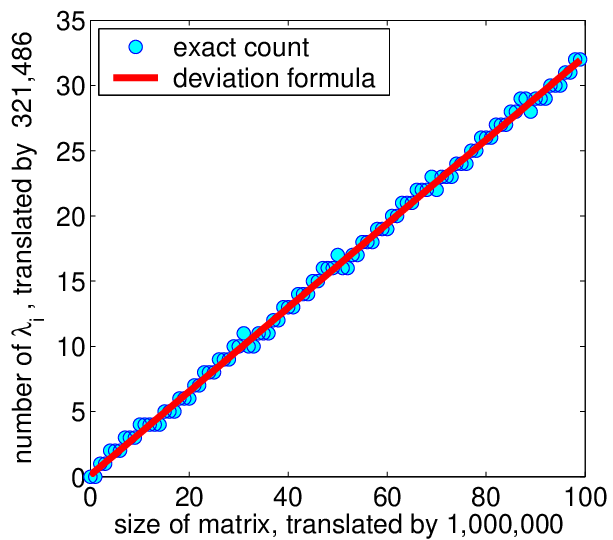
Refer to caption
Figure 2: Calculating the deviation in the interval I=[.2​.8]I=[.2~.8] for the β=∞\beta=\infty Hermite ensemble with sizes 106:1:(106+99)10^{6}:1:(10^{6}+99); circles represent the eigenvalue count minus the area under the semicircle over II; the solid line is the theoretical deviation given in (82)

Figure 2 plots the results of the experiment. The red line which contains the theoretical value of the intercept represents the best fit line to the data in the sense that the average vertical deviation is minimized.

6 Remarks and open problems

There are many object-counting (combinatorial) approaches to the study of traces of powers of random matrices; they depend on the matrix model, and on the polynomial whose trace is being computed. For example, the counting approach of [34] uses full matrix models (all entries are non-zero variables), and traces of powers (thus using the monomial basis, like we have done here), and counts paths in the complete graph of size nn. By contrast, in [26], the polynomials used are the shifted Chebyshev polynomials, and the objects counted are non-crossing annular partitions; the matrix models are still full. Here, we use tri/bidiagonal matrix models, consider the monomials, and count essentially paths with three types of steps (up, down, level) in the plane.

Though the objects we count here are simpler than in [26], our counting technique expresses the results in a less compact form than in [21] and [26]. In the latter two papers, the covariance matrix is diagonalized by the choice of polynomial basis, whereas in our paper it is obtained as full because we work with the monomials. There seems to be a trade-off between the simplicity of the object to be counted and the simplicity of the form in which the covariance matrix is expressed.

We would like to conjecture that by using a hybrid way of counting, for example, using the tridiagonal matrices and some of the techniques of [26], both the counting process and the resulting format of the answer could be simplified. The development of such a technique would be of great interest.

7 Acknowledgments

The authors would like to thank Alexei Borodin, Alexander Soshnikov, and Roland Speicher for many useful conversations on the subjects of global fluctuations, traces of powers of random matrices, and free probability. We also thank Inderjit Dhillon for providing Sturm sequence code, which we used for the histogramming of eigenvalues.

This research study has been conducted while Ioana Dumitriu was a Miller Research Fellow, sponsored by the Miller Institute for Basic Research in Sciences at U.C. Berkeley.

Finally, the authors would like to thank the National Science Foundation (DMS-0411962).

References

  • [1] Ludwig Arnold. On Wigner’s semicircle law for the eigenvalues of random matrices. Z. Wahrsch. Verw. Gebiete, 19:191–198, 1971.
  • [2] G. Ben Arous and A. Guionnet. Large Deviations for Wigner’s law and Voiculescu’s non-communtative entropy. PTRF, 108:517–548, 1997.
  • [3] T. Baker and Peter Forrester. The Calogero-Sutherland model and generalized classical polynomials. Commun.Math.Phys., 188:175–216, 1997.
  • [4] T. Cabanal-Duvillard. Fluctuations de la Loi Empirique de Grandes Matrices Aléatoires. Annales de l’Institut Henri Poincaré (B) Probab. Statist., 37:373–402, 2001.
  • [5] A.G. Constantine. Some noncentral distribution problems in multivariate analysis. Ann. Math. Statist., 34:1270–1285, 1963.
  • [6] A. Boutet de Montvel, L. Pastur, and M. Shcherbina. On the statistical mechanics approach in the random matrix theory:Integrated density of states. J. Stat. Phys., 79:585–611, 1995.
  • [7] A. Dembo, A. Guionnet, and O. Zeitouni. Moderate deviations for the spectral measure of certain random matrices. Ann. Inst. H. Poincaré(B) Probab. Statist., 39 (6):1013–1042, 2003.
  • [8] Patrick Desrosiers and Peter Forrester. Hermite and Laguerre β\beta-ensembles: asymptotic corrections to the eigenvalue density. Technical report, 2005. arxiv.org/PS_cache/math-ph/pdf/0509/0509021.pdf.
  • [9] Persi Diaconis and Mehrdad Shahshahani. On the eigenvalues of random matrices. J. Appl. Prob, 31:49–61, 1994.
  • [10] Ioana Dumitriu. Eigenvalue Statistics for the Beta-Ensembles. PhD thesis, Massachusetts Institute of Technology, 2003.
  • [11] Ioana Dumitriu and Alan Edelman. Matrix models for beta-ensembles. J. Math. Phys., 43:5830–5847, 2002.
  • [12] Ioana Dumitriu and Alan Edelman. Eigenvalues of Hermite and Laguerre ensembles: Large Beta Asymptotics. Ann. Inst. H. Poincaré (B) Probab. Statist., 41 (6):1083–1099, 2005.
  • [13] Ioana Dumitriu, Alan Edelman, and Gene Shuman. MOPS: Multivariate Orthogonal Polynomials (symbolically). 2004. Preprint found at lanl.arxiv.org/abs/math-ph/0409066.
  • [14] Freeman J. Dyson. The threefold way. Algebraic structures of symmetry groups and ensembles in Quantum Mechanics. J. Math. Phys., 3:1199–1215, 1963.
  • [15] Peter Forrester. Global fluctuation formulas and universal correlations for random matrices and log-gas systems at infinite density. Nuclear Phys. B, 435:421–429, 1995.
  • [16] Peter Forrester. Random Matrices. 2001. Preprint.
  • [17] F.R. Gantmacher and M.G. Krein. Oscillation Matrices and Kernels and Small Vibrations of Mechanical Systems (Revised English Edition). Amer. Math. Soc. Chelsea Publ., Amer. Math. Soc., Providence, R.I., 2002.
  • [18] A. Guionnet. Large deviations upper bounds and central limit theorems for non-commutative functionals of Gaussian large random matrices. Ann. Inst. H. Poincaré (B) Probab. Statist., 38:341–348, 2002.
  • [19] A. Guionnet and O. Zeitouni. Large deviations asymptotics for spherical integrals. J. Funct. Anal., 188 (2):461–515, 2002.
  • [20] Alan T. James. Distributions of matrix variates and latent roots derived from normal samples. Ann. Math. Stat., 35:475–501, 1964.
  • [21] Kurt Johansson. On fluctuations of random hermitian matrices. Duke Math. J., 91:151–203, 1998.
  • [22] Kurt Johansson. Shape fluctuations and random matrices. Commun. Math. Phys., 209:437–476, 2000.
  • [23] Iain M. Johnstone. On the distribution of the largest principal component. Ann. of Stat., 29(2):295–327, 2001.
  • [24] Dag Jonsson. Some limit theorems for the eigenvalues of a sample covariance matrix. J. Multivariate. Anal., 12:1–38, 1982.
  • [25] Rowan Killip and Irina Nenciu. Matrix Models for Circular Ensembles. International Mathematics Research Notices, 50:2665–2701, 2004.
  • [26] Timothy Kusalik, James A. Mingo, and Roland Speicher. Orthogonal Polynomials and Fluctuations of Random Matrices. Technical report, 2005. arxiv.org/abs/math.OA/0503169.
  • [27] I.G. Macdonald. Symmetric Functions and Hall Polynomials. Oxford University Press Inc, New York, 1995.
  • [28] V.A. Marčenko and L.A. Pastur. Distribution of eigenvalues for some sets of random matrices. Math USSR Sbornik, 1:457–483, 1967.
  • [29] Madan Lal Mehta. Random Matrices. Academic Press, Boston, second edition, 1991.
  • [30] Robb J. Muirhead. Aspects of Multivariate Statistical Theory. John Wiley & Sons, New York, 1982.
  • [31] H.D. Politzer. Random-matrix description of the distribution of mesoscopic conductance. Phys. Review B, 40:11917–11919, 1989.
  • [32] Jack W. Silverstein and Z.D. Bai. CLT of linear spectral statistics of large dimensional sample covariance matrices. preprint, 2003. Accepted for publication in Annals. of Probab.
  • [33] Alexander Soshnikov and Yakov Sinai. Central limit theorem for traces of large symmetric matrices with independent matrix elements. Bol. Soc. Bras. Mat., Nova Sr., 29:1–24, 1998.
  • [34] Alexander Soshnikov and Yakov Sinai. A Refinement of Wigner’s Semicircle Law in a Neighborhood of the Spectrum Edge for Random Symmetric Matrices. Func. Anal. and Appl., 32 (2):114–131, 1998.
  • [35] Roland Speicher. Combinatorial Aspects of Free Probability Theory. Lecture Notes, Freie Wahrscheinlichkeitstheorie, Goettingen, August 2005.
  • [36] Richard P. Stanley. Some combinatorial properties of Jack symmetric functions. Adv. in Math., 77:76–115, 1989.
  • [37] Richard P. Stanley. Enumerative Combinatorics, vol. 2. Cambridge University Press, 1999.
  • [38] Brian Sutton. The Stochastic Operator Approach to Random Matrix Theory. PhD thesis, Massachusetts Insitute of Technology, 2003.
  • [39] Craig A. Tracy and Harold Widom. Fredholm determinants, differential equations and matrix models. Commun. Math. Phys., 163:33–72, 1994.
  • [40] Craig A. Tracy and Harold Widom. On orthogonal and symplectic matrix ensembles. J. Stat. Phys., 92:809–835, 1996.
  • [41] Craig A. Tracy and Harold Widom. The distribution of the largest eigenvalue in the Gaussian ensembles. In Calogero-Moser-Sutherland Models, CRM Series in Mathematical Physics, volume 4, pages 461–472. Springer-Verlag, 2000.
  • [42] Eric W. Weisstein. ”Hermite Polynomial.” From MathWorld–A Wolfram Web Resource. http://mathworld.wolfram.com/HermitePolynomial.html.
  • [43] Eric W. Weisstein. ”Laguerre Polynomial.” From MathWorld–A Wolfram Web Resource. http://mathworld.wolfram.com/LaguerrePolynomial.html.
  • [44] Eugene P. Wigner. Characteristic vectors of bordered matrices with infinite dimensions. Ann. of Math., 62:548–564, 1955.
  • [45] Eugene P. Wigner. On the distribution of the roots of certain symmetric matrices. Ann. of Math., 67:325–327, 1958.
  • [46] J. Wishart. The generalized product moment distribution in samples from a normal multivariate population. Biometrika A, 20:32–43, 1928.