跳到论文正文
W Papers独立论文阅读器 arXiv:math-ph/0504083 论文正文 计算阅读时间 · 0%
引用这篇论文根据当前论文元数据生成,正式投稿前建议核对。


License: Assumed arXiv.org perpetual non-exclusive license
arXiv:math-ph/0504083v2 [math-ph] 11 Jul 2006

Point Interactions in Acoustics: One Dimensional
Models.

C. Cacciapuoti11 1 claudio.cacciapuoti@na.infn.it, R. Figari22 2 figari@na.infn.it, A. Posilicano33 3 andrea.posilicano@uninsubria.it

1,2Istituto Nazionale di Fisica Nucleare, Sezione di Napoli
Dipartimento di Scienze Fisiche
Università di Napoli Federico II,
Via Cintia 80126 Napoli, Italy

3Dipartimento di Fisica e Matematica
Università dell’Insubria
Via Valleggio 11, 22100 Como, Italy

Abstract

A one dimensional system made up of a compressible fluid and several mechanical oscillators, coupled to the acoustic field in the fluid, is analyzed for different settings of the oscillators array. The dynamical models are formulated in terms of singular perturbations of the decoupled dynamics of the acoustic field and the mechanical oscillators.

Detailed spectral properties of the generators of the dynamics are given for each model we consider. In the case of a periodic array of mechanical oscillators it is shown that the energy spectrum presents a band structure.

Introduction

In this paper we study the dynamics of a system consisting of one or more mechanical oscillators (the sources) coupled with the acoustic field they produce in the compressible fluid surrounding them.

Classical electromagnetism is perhaps the most well known case in theoretical physics where all attempts to construct a complete, covariant, causal, divergence free theory for the evolution of the fields together with their sources were unsuccessful up to now (in fact it is hard to say that there is a single case in Classical or in Quantum Physics in which this problem was completely solved).

Whereas theories with extended rigid charges are quite well understood both at the classical and the quantum level (see e.g. the recent book [S] for a systematic introduction to the subject and for a long list of references), there is no mathematically consistent theory of point charges interacting with their own electromagnetic field. Indeed Newton equations with Lorentz force require the fields to be evaluated at the particle positions, and this produces infinities due to the presence of the point-like sources. These difficulties directly lead to the need of mass renormalization. In his seminal paper Dirac [D] (also see [IW], [K], [M]), without using Lorentz force but exploiting the conservation of energy and momentum and considering their flow through a thin tube of radius rr, derived an equation for the motion of a charged point particle (the Lorentz-Dirac equation). As Dirac himself pointed out the equation obtained in the limit r↓0r\downarrow 0, together with the mass renormalization, leads to the presence of runaway solutions, i.e. solutions for which the acceleration increases beyond any bound even in the absence of external fields.

An approach based on the theory of singular perturbations of the free dynamics was initiated in [NP1] and [NP2] for the case of classical electrodynamics of a point particle in the dipole (or linearized) case. Here the generator of the limit dynamics of both the field and the particle appears to be a singular perturbation of the generator of the free dynamics. The phenomenological mass plays the role of the parameter describing a suitable family of self-adjoint extensions and the boundary condition naturally appearing in the domain of the generator results to be nothing else that a regularized (and linearized) version of the usual velocity-momentum relation in the presence of an electromagnetic field. In this framework runaway solutions are unavoidable because a negative eigenvalue appears in the spectrum of the generator after mass renormalization.

Our interest in a similar problem in acoustics was prompted by the appearance in 1999 of a paper by J. D. Templin [T]. In that paper the author analyzed the dynamics of a simple model of a spherical oscillator interacting with the acoustic field it generates. The existence of a spherically symmetric radiation field (the acoustic monopole) makes the acoustic case significantly different from the electromagnetic one. Moreover the pressure field at the surface of the sphere completely characterizes the contact forces responsible of the interaction between source and field in the acoustic case.

Templin performed a detailed analysis of the field emitted by the acoustic monopole, explicitly computing both its radiation and near-field components. He noticed that a deduction of the reaction field obtained from the emitted radiation power, therefore neglecting the near field component, brings to an equation for the radius of the oscillating sphere showing runaway solutions.

In analogy with what was done for the electromagnetic case in [NP1] we want to provide a formalization of the problem of a finite or infinite number of oscillators coupled with their acoustic field in terms of singular perturbations of the generator of the free dynamics.

In this paper we will consider only the one dimensional case. In the abstract setting we will work in the physical model of interaction between sources and field will appear as the only possible extension of the free dynamics. The generalization to three dimensions is not straightforward. From one side a model of a physically relevant, symmetric, mechanical oscillator with finite degrees of freedom is lacking. On the other side point perturbations of the free dynamics are much more singular in higher dimensions. We plan to discuss the three dimensional case in further work.

We want to stress an aspect of the dynamical system we analyze here which was extensively studied in different contexts. As an immediate consequence of the third Newton’s law and of the assumption of persistent contact between the fluid and the surface of the oscillators, the total energy, sum of the (positive) energy of the acoustic field Ea​cE_{ac} and the (positive) energy of the oscillators Eo​s​cE_{osc}, is a constant of motion. As an immediate consequence one can exclude the existence of runaway solutions in this case. Moreover, lacking a mechanism of reflection of the acoustic waves at some exterior boundary, the motion of the oscillators should be damped and the energy should finally diffuse over the field degrees of freedom, for almost every initial condition. The situation is reminiscent of the one investigated in [SW1], [SW2] and [SW3] about the diffusion of energy from bound states to continuous states triggered by time dependent perturbations in quantum and classical systems. In our system there is no external potential the interaction being given by internal forces.

This paper is organized as follows.

In section 1 we introduce a list of notation and we briefly recall the equations for the acoustic field. Afterwards we exemplify the problem of the interaction between the field and a source in the completely solvable case of a single wall attracted toward the origin by a linear restoring force.

In section 2 we analyze the case of a finite number of sources in the framework of the possible extensions of the free dynamics outside the points where the sources are placed.

In section 3 we generalize the construction to the case of infinitely many sources and study the case of sources periodically placed on the real line. We give detailed results on the characteristic band structure of the spectrum of the generator of the dynamics.

To the best of our knowledge this kind of systems of oscillators coupled with the acoustic field was never proposed and solved. A remark on the band structure of a similar model is in [GS].

1 The acoustic monopole in one dimension

We give a detailed description of our model in the simplest case of one oscillator coupled with the acoustic field.

Consider an infinite pipe filled with a non viscous, compressible fluid. We suppose that there is no friction between the fluid and the pipe and we choose a coordinate system with the xx-axis parallel to the axis of the pipe. The mechanical oscillator is made up of a very thin wall of mass MM positioned in the pipe perpendicularly to the axis in x=0x=0. The thin wall is connected to a spring of elastic constant KK. We analyze only one dimensional cases, hence the acoustic field is described by the pressure field p⁡(x,t)p(x,t) and the velocity field v⁡(x,t)v(x,t). The motion of the mechanical oscillator is described through the position and the velocity of the thin wall.

The field p⁡(x,t)p(x,t) represents deviations of the pressure in the point xx at time tt with respect to an equilibrium pressure P0P_{0}. In the linearized acoustics regime the continuity equation, the Newton’s second law and the adiabatic equation of state read

∂ρ∂t+ρ0​∂v∂x=0,ρ0​∂v∂t=−∂p∂x,p=a2​ρ,\frac{\partial{\rho}}{\partial{t}}+\rho_{0}\frac{\partial{v}}{\partial{x}}=0\;,\quad\rho_{0}\frac{\partial{v}}{\partial{t}}=-\frac{\partial{p}}{\partial{x}}\;,\quad p=a^{2}\rho\;, (1.1)

where ρ⁡(x,t)\rho(x,t) is the deviation of the density in the point xx at time tt with respect to the equilibrium density ρ0\rho_{0} and aa is the velocity of sound in the fluid.

Then we have for p⁡(x,t)p(x,t) and v⁡(x,t)v(x,t) the following coupled differential equations

∂p∂t=−a2​ρ0​∂v∂x,∂v∂t=−1ρ0​∂p∂x.\frac{\partial{p}}{\partial{t}}=-a^{2}\rho_{0}\frac{\partial{v}}{\partial{x}}\;,\quad\frac{\partial{v}}{\partial{t}}=-\frac{1}{\rho_{0}}\frac{\partial{p}}{\partial{x}}\;. (1.2)

We consider only small oscillations of the thin wall around its equilibrium position x=0x=0, we indicate with y⁡(t)y(t) the displacement of the wall from its equilibrium position at time tt and we suppose that the wall remains always in contact with the fluid

v⁡(y⁡(t),t)=d​y​(t)d​t∀t≥0.v(y(t),t)=\frac{dy(t)}{dt}\qquad\forall t\geq 0\;. (1.3)

Notice that we consider a wall of zero thickness. We make the approximation v⁡(y⁡(t),t)≃v⁡(0,t)v(y(t),t)\simeq v(0,t) and condition (1.3) becomes

v⁡(0,t)=d​y​(t)d​t∀t≥0.v(0,t)=\frac{dy(t)}{dt}\qquad\forall t\geq 0\;. (1.4)

The equation of motion for the position of the thin wall y⁡(t)y(t) is

M​y¨​(t)=−K​y​(t)−S⁡(p⁡(0+,t)−p⁡(0−,t))M\ddot{y}(t)=-Ky(t)-S\left(p(0^{+},t)-p(0^{-},t)\right) (1.5)

where SS is the area of the transverse section of the pipe and we made the approximation p⁡(y±​(t),t)≃p⁡(0±,t)p(y^{\pm}(t),t)\simeq p(0^{\pm},t).

The total energy of the system is given by

Et​o​t=Ea​c+Eo​s​cE_{tot}=E_{ac}+E_{osc} (1.6)

with

Ea​c\displaystyle E_{ac} =S2​a2​ρ0​∫−∞∞p​(x)2​𝑑x+S​ρ02​∫−∞∞v​(x)2​𝑑x\displaystyle=\frac{S}{2a^{2}\rho_{0}}\int_{-\infty}^{\infty}p(x)^{2}dx+\frac{S\rho_{0}}{2}\int_{-\infty}^{\infty}v(x)^{2}dx (1.7)
Eo​s​c\displaystyle E_{osc} =K2​y2+M2​y˙2,\displaystyle=\frac{K}{2}y^{2}+\frac{M}{2}\dot{y}^{2}\,, (1.8)

Ea​cE_{ac} is the energy stored in the acoustic field while Eo​s​cE_{osc} is the energy of the mechanical oscillator.

As the system is isolated the energy is constant. The motion of the wall produces acoustic waves thus transferring continuously energy from the oscillator to the acoustic field. One then expects that y⁡(t)y(t) decreases to zero when t→∞t\to\infty.

In spite of being a simple exercise, the exact computation of the solution of problem (1.2), (1.4), (1.5) and, in turn, of the damping rate of the oscillations rarely appears in textbooks.

In the following we give the solution of the Cauchy problem of coupled ordinary and partial differential equations with time dependent boundary conditions

{∂p∂t=−a2​ρ0​∂v∂x∀t≥0​∀x∈ℝ\{0}∂v∂t=−1ρ0​∂p∂x∀t≥0​∀x∈ℝ\{0}y¨​(t)=−ω02​y​(t)−SM​(p⁡(0+,t)−p⁡(0−,t))∀t≥0p⁡(x,0)=f⁡(x)∀x∈ℝ\{0}v⁡(x,0)=g⁡(x)∀x∈ℝ\{0}y⁡(0)=y0y˙​(0)=y˙0v​(0,t)=y˙​(t)∀t≥0\begin{cases}\displaystyle\frac{\partial{p}}{\partial{t}}=-a^{2}\rho_{0}\frac{\partial{v}}{\partial{x}}&\forall t\geq 0\;\forall x\in\mathbb{R}\backslash\{0\}\\ \displaystyle\frac{\partial{v}}{\partial{t}}=-\frac{1}{\rho_{0}}\frac{\partial{p}}{\partial{x}}&\forall t\geq 0\;\forall x\in\mathbb{R}\backslash\{0\}\\ \ddot{y}(t)=-\omega_{0}^{2}y(t)-\displaystyle\frac{S}{M}\left(p(0^{+},t)-p(0^{-},t)\right)&\forall t\geq 0\\ p(x,0)=f(x)&\forall x\in\mathbb{R}\backslash\{0\}\\ v(x,0)=g(x)&\forall x\in\mathbb{R}\backslash\{0\}\\ y(0)=y_{0}&\\ \dot{y}(0)=\dot{y}_{0}&\\ v(0,t)=\dot{y}(t)&\forall t\geq 0\end{cases} (1.9)

where f⁡(x)f(x) and g⁡(x)g(x) are two real functions and ω02=K/M\omega_{0}^{2}=K/M.

Suppose that

f(x)∈C02(ℝ);g(x)∈C02(ℝ)andy0=1ω02​ρ0f′(0);y˙0=g(0),f(x)\in C_{0}^{2}(\mathbb{R})\,;\;g(x)\in C_{0}^{2}(\mathbb{R})\quad\textrm{and}\quad y_{0}=\displaystyle\frac{1}{\omega_{0}^{2}\rho_{0}}f^{\prime}(0)\,;\;\dot{y}_{0}=g(0)\,, (1.10)

then the solution of problem (1.9) reads

p⁡(x,t)\displaystyle p(x,t) =pf​(x,t)+a​ρ0​sgn​(x)​Y​(t−|x|a)\displaystyle=p_{f}(x,t)+a\rho_{0}\;\text{\rm sgn}(x)Y\left(t-\frac{|x|}{a}\right) (1.11)
v⁡(x,t)\displaystyle v(x,t) =vf​(x,t)+Y⁡(t−|x|a)\displaystyle=v_{f}(x,t)+Y\left(t-\frac{|x|}{a}\right) (1.12)
y⁡(t)\displaystyle y(t) =−v˙f​(0,t)ω02+∫0tF⁡(t′)β+​eβ+​(t−t′)​d​t′−∫0tF⁡(t′)β−​eβ−​(t−t′)​d​t′β+−β−\displaystyle=-\frac{\dot{v}_{f}(0,t)}{\omega_{0}^{2}}+\frac{\displaystyle\int_{0}^{t}\frac{F(t^{\prime})}{\beta_{+}}e^{\beta_{+}(t-t^{\prime})}dt^{\prime}-\int_{0}^{t}\frac{F(t^{\prime})}{\beta_{-}}e^{\beta_{-}(t-t^{\prime})}dt^{\prime}}{\beta_{+}-\beta_{-}} (1.13)

where pf​(x,t)p_{f}(x,t) and vf​(x,t)v_{f}(x,t) are solution of the wave equation in (−∞,+∞)(-\infty,+\infty) with initial conditions f⁡(x)f(x) and g⁡(x)g(x)

pf​(x,t)\displaystyle p_{f}(x,t) =f⁡(x−a​t)+f⁡(x+a​t)2+a​ρ02​(g⁡(x−a​t)−g⁡(x+a​t))\displaystyle=\frac{f(x-at)+f(x+at)}{2}+\frac{a\rho_{0}}{2}\left(g(x-at)-g(x+at)\right) (1.14)
vf​(x,t)\displaystyle v_{f}(x,t) =g⁡(x−a​t)+g⁡(x+a​t)2+12​a​ρ0​(f⁡(x−a​t)−f⁡(x+a​t)),\displaystyle=\frac{g(x-at)+g(x+at)}{2}+\frac{1}{2a\rho_{0}}\left(f(x-at)-f(x+at)\right)\,,
F⁡(t)=−v¨f​(0,t)−ω02​vf​(0,t)F(t)=-\ddot{v}_{f}(0,t)-\omega_{0}^{2}v_{f}(0,t) (1.15)

and

Y⁡(t)=∫0tF⁡(t′)​eβ+​(t−t′)​d​t′−∫0tF⁡(t′)​eβ−​(t−t′)​d​t′β+−β−Y(t)=\frac{\displaystyle\int_{0}^{t}F(t^{\prime})e^{\beta_{+}(t-t^{\prime})}dt^{\prime}-\int_{0}^{t}F(t^{\prime})e^{\beta_{-}(t-t^{\prime})}dt^{\prime}}{\beta_{+}-\beta_{-}} (1.16)

with β±=(−γ±γ2−4​ω02)/2\beta_{\pm}=(-\gamma\pm\sqrt{\gamma^{2}-4\omega_{0}^{2}})/2 with γ=2​a​ρ0​S/M\gamma=2a\rho_{0}S/M.

By conditions (1.10) one easily obtain that y⁡(t)y(t) and y˙​(t)\dot{y}(t) are both continuous and decrease exponentially to zero with decay constant τ=γ/2\tau=\gamma/2.

2 Singular perturbations of the free dynamics

In this section we present a generalization of problem (1.9) formulated in terms of a unitary flow on a space of finite energy.

Let us consider a system of nn thin walls positioned in a pipe, perpendicularly to its axis. Let 𝒮={s1,…,sn}⊂ℝ\mathcal{S}=\left\{s_{1},\dots,s_{n}\right\}\subset\mathbb{R} be the set of equilibrium positions of the thin walls. The ii-th thin wall, placed in sis_{i}, has mass MiM_{i} and is connected to a spring of elastic constant KiK_{i}. The acoustic field is described by the pressure field pp and the velocity field vv. The motion of the walls is described by the displacements yjy_{j} from their equilibrium positions and by the corresponding velocities zjz_{j}.

The generator of the dynamics, A^\hat{A}, will be defined as a singular perturbation of the skew-adjoint operator AA generating the uncoupled evolution of the acoustic field and of the oscillators.

The system of first order differential equations

∂p∂t\displaystyle\frac{\partial p}{\partial t} =−a2​ρ0​∂v∂x\displaystyle=-a^{2}\rho_{0}\,\frac{\partial v}{\partial x} ∀x∈ℝ\displaystyle\forall x\in\mathbb{R} (2.1)
∂v∂t\displaystyle\frac{\partial v}{\partial t} =−1ρ0​∂p∂x\displaystyle=-\frac{1}{\rho_{0}}\,\frac{\partial p}{\partial x} ∀x∈ℝ\displaystyle\forall x\in\mathbb{R} (2.2)
d​yjd​t\displaystyle\frac{dy_{j}}{dt} =zj\displaystyle=z_{j} 1≤j≤n\displaystyle 1\leq j\leq n (2.3)
d​zjd​t\displaystyle\frac{dz_{j}}{dt} =−KjMj​yj\displaystyle=-\frac{K_{j}}{M_{j}}\,y_{j} 1≤j≤n\displaystyle 1\leq j\leq n (2.4)

describes, in the linear approximation, the independent evolution of nn mechanical oscillators and of the acoustic field.

We want to show first how equations (2.1) - (2.4) define an unitary flow in a complex Hilbert space. To this aim let us consider equations (2.1) - (2.4) for complex functions vv, pp, yjy_{j}, zjz_{j} of position and time.

The set of all the displacements and velocities will be represented respectively by the vectors in ℂn\mathbb{C}^{n}

y¯=y1​e¯1+⋯+yn​e¯n,z¯=z1​e¯1+⋯+zn​e¯n,\underline{y}=y_{1}\underline{e}_{1}+\dots+y_{n}\underline{e}_{n}\,,\quad\underline{z}=z_{1}\underline{e}_{1}+\dots+z_{n}\underline{e}_{n}\,, (2.5)

where e¯1,…,e¯n\underline{e}_{1},\dots,\underline{e}_{n} is the canonical orthonormal basis in ℂn\mathbb{C}^{n}.

Let us denote by L2​(ℝ)L^{2}(\mathbb{R}) the space of square-integrable functions on the real line. H¯1​(ℝ)\bar{H}^{1}(\mathbb{R}) indicates the homogeneous Sobolev space of locally square-integrable functions with square-integrable (distributional) derivative, and H1​(ℝ)H^{1}(\mathbb{R}) the usual Sobolev space H1​(ℝ):=H¯1​(ℝ)∩L2​(ℝ)H^{1}(\mathbb{R}):=\bar{H}^{1}(\mathbb{R})\cap L^{2}(\mathbb{R}).

Therefore the linear operator AA in L2​(ℝ)⊕L2​(ℝ)⊕ℂn⊕ℂnL^{2}(\mathbb{R})\oplus L^{2}(\mathbb{R})\oplus\mathbb{C}^{n}\oplus\mathbb{C}^{n} generating the dynamics (2.1) - (2.4) is defined by

A:H1​(ℝ)⊕H1​(ℝ)⊕ℂn⊕ℂn→L2​(ℝ)⊕L2​(ℝ)⊕ℂn⊕ℂnA:H^{1}(\mathbb{R})\oplus H^{1}(\mathbb{R})\oplus\mathbb{C}^{n}\oplus\mathbb{C}^{n}\to L^{2}(\mathbb{R})\oplus L^{2}(\mathbb{R})\oplus\mathbb{C}^{n}\oplus\mathbb{C}^{n} (2.6)
A(p,v,y¯,z¯):=(−a2ρ0d​vd​x,−1ρ0d​pd​x,z¯,−∑1≤j≤nKjMjyje¯j),A(p,v,\underline{y},\underline{z}):=\left(-a^{2}\rho_{0}\,\frac{dv}{dx},\,-\frac{1}{\rho_{0}}\,\frac{dp}{dx},\,\underline{z},\,-\sum_{1\leq j\leq n}\frac{K_{j}}{M_{j}}\,y_{j}\underline{e}_{j}\right)\,, (2.7)

where aa, ρ0\rho_{0}, KjK_{j}, MjM_{j}, 1≤j≤n1\leq j\leq n, are the positive real constants representing the physical parameters.

In the following a capital Greek letter will indicate a generic vector (p,v,y¯,z¯)(p,v,\underline{y},\underline{z}) in L2​(ℝ)⊕L2​(ℝ)⊕ℂn⊕ℂnL^{2}(\mathbb{R})\oplus L^{2}(\mathbb{R})\oplus\mathbb{C}^{n}\oplus\mathbb{C}^{n}.

AA is a real operator, i.e. it preserves the (physical) linear subspace of real elements

{(p,v,y¯,z¯):p(x)∈ℝ,v(x)∈ℝ,y¯∈ℝn,z¯∈ℝn}.\left\{(p,v,\underline{y},\underline{z})\,:\,p(x)\in\mathbb{R},\ v(x)\in\mathbb{R},\ \underline{y}\in\mathbb{R}^{n},\ \underline{z}\in\mathbb{R}^{n}\right\}\,. (2.8)

AA is skew-symmetric with respect to the scalar product

⟨⟨Ψ1,Ψ2⟩⟩≡1a2​ρ0​⟨p1,p2⟩+ρ0​⟨v1,v2⟩+1S​∑1≤j≤nKj​y¯1​j​y2​j+Mj​z¯1​j​z2​j,\langle\langle\Psi_{1},\Psi_{2}\rangle\rangle\equiv\frac{1}{a^{2}\rho_{0}}\,\langle p_{1},p_{2}\rangle+\rho_{0}\langle v_{1},v_{2}\rangle+\frac{1}{S}\sum_{1\leq j\leq n}{K_{j}}\,\bar{y}_{1j}y_{2j}+{M_{j}}\,\bar{z}_{1j}z_{2j}\,, (2.9)

where ⟨⋅,⋅⟩\langle\cdot\,,\cdot\rangle indicates the standard scalar product in L2​(ℝ)L^{2}(\mathbb{R}), SS is the area of the transverse section of the pipe and - denotes complex conjugation. L2​(ℝ)⊕L2​(ℝ)⊕ℂn⊕ℂnL^{2}(\mathbb{R})\oplus L^{2}(\mathbb{R})\oplus\mathbb{C}^{n}\oplus\mathbb{C}^{n} is a Hilbert space with the scalar product (2.9).

The square norm of a vector Ψ\Psi, ‖Ψ‖2=⟨⟨Ψ,Ψ⟩⟩\|\Psi\|^{2}=\langle\langle\Psi,\Psi\rangle\rangle, defines the total energy of the system in the state Ψ\Psi

Et​o​t=S2​‖Ψ‖2=Ea​c+Eo​s​cE_{tot}=\frac{S}{2}\|\Psi\|^{2}=E_{ac}+E_{osc} (2.10)

where Ea​cE_{ac} is the energy stored in the acoustic field while Eo​s​cE_{osc} is the energy of the oscillators

Ea​c=S2​a2​ρ0​⟨p,p⟩+ρ0​S2​⟨v,v⟩;Eo​s​c=12​∑1≤j≤n(Kj​|yj|2+Mj​|zj|2).E_{ac}=\frac{S}{2a^{2}\rho_{0}}\,\langle p,p\rangle+\frac{\rho_{0}S}{2}\langle v,v\rangle\;;\quad E_{osc}=\frac{1}{2}\sum_{1\leq j\leq n}\left({K_{j}}|y_{j}|^{2}+{M_{j}}\,|z_{j}|^{2}\right)\,. (2.11)

For any ζ∈ℂ\i​ℝ\zeta\in\mathbb{C}\backslash i\mathbb{R} the resolvent of AA is

(−A+ζ)−1(p,v,y¯,z¯)=(ρ0(−d2d​x2+ζ2a2)−1(−d​vd​x+ζa2​ρ0p),\displaystyle(-A+\zeta)^{-1}(p,v,\underline{y},\underline{z})=\left(\rho_{0}\left(-\frac{d^{2}}{dx^{2}}+\frac{\zeta^{2}}{a^{2}}\right)^{-1}\left(-\frac{dv}{dx}+\frac{\zeta}{a^{2}\rho_{0}}\,p\right),\right. (2.12)
1a2​ρ0​(−d2d​x2+ζ2a2)−1​(−d​pd​x+ζ​ρ0​v),∑1≤j≤nMj​zj+ζ​Mj​yjKj+ζ2​Mj​e¯j,\displaystyle\frac{1}{a^{2}\rho_{0}}\,\left(-\frac{d^{2}}{dx^{2}}+\frac{\zeta^{2}}{a^{2}}\right)^{-1}\left(-\frac{dp}{dx}+\zeta\rho_{0}v\right),\ \sum_{1\leq j\leq n}\frac{M_{j}z_{j}+\zeta M_{j}y_{j}}{K_{j}+\zeta^{2}M_{j}}\,\underline{e}_{j}\,,
OPEN∑1≤j≤n−Kj​yj+ζ​Mj​zjKj+ζ2​Mj​e¯j).\displaystyle\left.\sum_{1\leq j\leq n}\frac{-K_{j}y_{j}+\zeta M_{j}z_{j}}{K_{j}+\zeta^{2}M_{j}}\,\underline{e}_{j}\right)\,.

Since

Ran(−A±1)=L2​(ℝ)⊕L2​(ℝ)⊕ℂn⊕ℂn,\text{\rm Ran$(-A\pm 1)$}=L^{2}(\mathbb{R})\oplus L^{2}(\mathbb{R})\oplus\mathbb{C}^{n}\oplus\mathbb{C}^{n}\,, (2.13)

AA is skew-adjoint. Moreover the essential spectrum of AA is purely absolutely continuous and

σe​s​s(A)=σa​c(A)=iℝ,σp​p(A)={±iKjMj, 1≤j≤n}.\sigma_{ess}(A)=\sigma_{ac}(A)=i\mathbb{R}\,,\quad\sigma_{pp}(A)=\left\{\pm i\,\sqrt{\frac{K_{j}}{M_{j}}}\,,\ 1\leq j\leq n\right\}\,. (2.14)

Being skew-adjoint the operator AA describes, by Stone theorem, the uncoupled evolution of the acoustic field and of the oscillators through the unitary flow exp⁡t​A\exp tA corresponding to the Cauchy problem for the first order differential equation

dd​t​Ψ​(t)=A​Ψ​(t)\frac{d}{dt}\Psi(t)=A\Psi(t) (2.15)

which is equivalent to the system written at the beginning of the section.

Now we consider the linear operator A0A_{0} obtained by restricting AA on the set of vectors in its domain satisfying:

{v(sj)=zj,1≤j≤n}\left\{v(s_{j})=z_{j}\,,\quad 1\leq j\leq n\right\} (2.16)

which represents the kinematic constraint (1.4) at each thin wall. A0A_{0} is a closed, densely defined, skew-symmetric linear operator with defect indices (n,n)(n,n). We want to characterize the skew-adjoint extensions of A0A_{0}. The family of extensions of A0A_{0} can be parameterized by relations K⊂ℂn⊕ℂnK\subset\mathbb{C}^{n}\oplus\mathbb{C}^{n} which are skew-symmetric, i.e. such that K=(ℐ​K)⟂K=({\mathscr{I}}K)^{\perp}, where ℐ⁡(z¯1,z¯2):=(z¯2,z¯1){\mathscr{I}}(\underline{z}_{1},\underline{z}_{2}):=(\underline{z}_{2},\underline{z}_{1}) (see e.g. [GG], Theorem 1.6, chapter 3, for the analogous self-adjoint case). A skew-symmetric relation in ℂn⊕ℂn\mathbb{C}^{n}\oplus\mathbb{C}^{n} extends the notion of the graph of a skew-symmetric operator Θ:ℂn→ℂn\Theta:\mathbb{C}^{n}\to\mathbb{C}^{n} through the relation K={(z¯,Θ​z¯),z¯∈ℂn}K=\{(\underline{z},\Theta\underline{z})\,,\ \underline{z}\in\mathbb{C}^{n}\}. In order to be a candidate to describe the interacting dynamics of the system under analysis a skew-adjoint extension of A0A_{0} must be local and real i.e. it must generate a coupling between the fields evaluated in sjs_{j} and the jj-th oscillator, 1≤j≤n1\leq j\leq n, and it must preserve the linear space of physical data defined in (2.8). The only admissible extension different from AA itself will be the one corresponding to the graph of the zero operator, Θ=0\Theta=0. The next theorem completely characterizes such an extension:

Theorem 2.1.

The only local, real and skew-adjoint extension of A0A_{0} is given by

A^:D⁡(A^)⊂L2​(ℝ)⊕L2​(ℝ)⊕ℂn⊕ℂn→L2​(ℝ)⊕L2​(ℝ)⊕ℂn⊕ℂn,\hat{A}:D(\hat{A})\subset L^{2}(\mathbb{R})\oplus L^{2}(\mathbb{R})\oplus\mathbb{C}^{n}\oplus\mathbb{C}^{n}\to L^{2}(\mathbb{R})\oplus L^{2}(\mathbb{R})\oplus\mathbb{C}^{n}\oplus\mathbb{C}^{n}\,, (2.17)
D(A^)={\displaystyle D(\hat{A})=\{ Ψ≡(p,v,y¯,z¯):p∈L2(ℝ)∩H1(ℝ\𝒮),v∈H1(ℝ),y¯∈ℂn,\displaystyle\Psi\equiv(p,v,\underline{y},\underline{z})\,:\,p\in L^{2}(\mathbb{R})\cap H^{1}(\mathbb{R}\backslash\mathcal{S}),\,v\in H^{1}(\mathbb{R}),\ \underline{y}\in\mathbb{C}^{n}, (2.18)
z¯∈ℂn,p(si+)−p(si−)=σi,v(sj)=zj,σ¯∈ℂn},\displaystyle\underline{z}\in\mathbb{C}^{n},\ p(s_{i}^{+})-p(s_{i}^{-})=\sigma_{i},\ v(s_{j})=z_{j},\ \underline{\sigma}\in\mathbb{C}^{n}\}\,,
A^​(p,v,y¯,z¯):=\displaystyle\hat{A}(p,v,\underline{y},\underline{z}):= (2.19)
:=(−a2ρ0d​vd​x,−1ρ0d​p0d​x,z¯,−∑1≤j≤n(KjMjyj+SMjσj)e¯j).\displaystyle:=\left(-a^{2}\rho_{0}\,\frac{dv}{dx},\,-\frac{1}{\rho_{0}}\,\frac{dp_{0}}{dx},\,\underline{z},\,-\sum_{1\leq j\leq n}\left(\frac{K_{j}}{M_{j}}\,y_{j}+\frac{S}{M_{j}}\,\sigma_{j}\right)\,\underline{e}_{j}\right)\,.

Here p0∈H¯1​(ℝ)p_{0}\in\bar{H}^{1}(\mathbb{R}),

p0​(x):=p⁡(x)−12​∑1≤j≤nσj​sgn​(x−sj),p_{0}(x):=p(x)-\frac{1}{2}\sum_{1\leq j\leq n}\sigma_{j}\,\text{\rm sgn}(x-s_{j})\,, (2.20)

denotes the regular part of pp. The resolvent of A^\hat{A} is given by

(−A^+ζ)−1=(−A+ζ)−1+∑1≤i,j≤n(Γ​(ζ)−1)i​j​Gζi⊗G˘ζ¯j,ζ∈ℂ\i​ℝ,(-\hat{A}+\zeta)^{-1}=(-A+\zeta)^{-1}+\sum_{1\leq i,j\leq n}\left(\Gamma(\zeta)^{-1}\right)_{ij}\,G^{i}_{\zeta}\otimes\breve{G}^{j}_{\bar{\zeta}}\,,\qquad\zeta\in\mathbb{C}\backslash i\mathbb{R}\,, (2.21)

where

Γ​(ζ)i​j:=−ζ⁡(±e∓ζ|si−sj|/a2​a​ρ0​ζ+S​δi​jKj+ζ2​Mj),±Reζ>0\Gamma(\zeta)_{ij}:=-\zeta\left(\pm\frac{e^{\mp\zeta|s_{i}-s_{j}|/a}}{2a\rho_{0}\zeta}+\frac{S\delta_{ij}}{K_{j}+\zeta^{2}M_{j}}\right)\,,\quad\text{\rm$\pm$Re$\,\zeta>0$} (2.22)

and

G˘ζj​(x)=(𝒢ζ′​(x−sj),ζa2​ρ0​𝒢ζ​(x−sj),SKj+ζ2​Mj​e¯j,−ζ​SKj+ζ2​Mj​e¯j),\breve{G}_{\zeta}^{j}(x)=\left(\mathcal{G}_{\zeta}^{\prime}(x-s_{j})\,,\frac{\zeta}{a^{2}\rho_{0}}\,\mathcal{G}_{\zeta}(x-s_{j})\,,\frac{S}{K_{j}+\zeta^{2}M_{j}}\,\underline{e}_{j}\,,\ \frac{-\zeta S}{K_{j}+\zeta^{2}M_{j}}\,\underline{e}_{j}\right)\,, (2.23)
Gζj​(x)=(−𝒢ζ′​(x−sj),ζa2​ρ0​𝒢ζ​(x−sj),−SKj+ζ2​Mj​e¯j,−ζ​SKj+ζ2​Mj​e¯j),G_{\zeta}^{j}(x)=\left(-\mathcal{G}_{\zeta}^{\prime}(x-s_{j})\,,\frac{\zeta}{a^{2}\rho_{0}}\,\mathcal{G}_{\zeta}(x-s_{j})\,,\frac{-S}{K_{j}+\zeta^{2}M_{j}}\,\underline{e}_{j}\,,\ \frac{-\zeta S}{K_{j}+\zeta^{2}M_{j}}\,\underline{e}_{j}\right)\,, (2.24)
𝒢ζ(x)=±a2​ζe∓ζ|x|/a,𝒢ζ′(x)=−12sgn(x)e∓ζ|x|/a,±Reζ>0.\mathcal{G}_{\zeta}(x)=\pm\frac{a}{2\zeta}\,e^{\mp\zeta|x|/a}\,,\quad\mathcal{G}_{\zeta}^{\prime}(x)=-\frac{1}{2}\,\text{\rm sgn}(x)\,e^{\mp\zeta|x|/a}\,,\quad\text{\rm$\pm$Re$\,\zeta>0$}\,. (2.25)
Proof.

Since i​A0iA_{0} is a closed, densely defined, symmetric operator with defect indices (n,n)(n,n), all its self-adjoint extensions can be obtained by the famed von Neumann theory on self-adjoint extensions (see e.g. Theorem X.2 in [RS2]). However, since A0A_{0} is obtained by restricting the skew-adjoint operator AA to the kernel of the continuous, surjective linear operator

τ:H1​(ℝ)⊕H1​(ℝ)⊕ℂn⊕ℂn→ℂn,\tau:H^{1}(\mathbb{R})\oplus H^{1}(\mathbb{R})\oplus\mathbb{C}^{n}\oplus\mathbb{C}^{n}\to\mathbb{C}^{n}\,, (2.26)
τ⁡(p,v,y¯,z¯):=∑1≤j≤n(v⁡(sj)−zj)​e¯j,\tau(p,v,\underline{y},\underline{z}):=\sum_{1\leq j\leq n}(v(s_{j})-z_{j})\,\underline{e}_{j}\,, (2.27)

it is easier to make use of the (equivalent) procedure developed in [P1] (also see the appendix in [P2] for a compact review). Here below we provide the (almost) self-contained construction of the skew-adjoint extensions of A0A_{0} by using such a procedure.

Given the map τ\tau we can define the bounded linear operator

G˘​(ζ):=τ​(−A+ζ)−1:L2​(ℝ)⊕L2​(ℝ)⊕ℂn⊕ℂn→ℂn.\breve{G}(\zeta):=\tau(-A+\zeta)^{-1}:L^{2}(\mathbb{R})\oplus L^{2}(\mathbb{R})\oplus\mathbb{C}^{n}\oplus\mathbb{C}^{n}\to\mathbb{C}^{n}\,. (2.28)

By the relation

G˘​(ζ)​(p,v,y¯,z¯)=∑1≤j≤n⟨⟨G˘ζ¯j,(p,v,y¯,z¯)⟩⟩​e¯j,1≤j≤n,\breve{G}(\zeta)(p,v,\underline{y},\underline{z})=\sum_{1\leq j\leq n}\langle\langle\breve{G}^{j}_{\bar{\zeta}},(p,v,\underline{y},\underline{z})\rangle\rangle\,\underline{e}_{j}\,,\quad 1\leq j\leq n\,, (2.29)

G˘​(ζ)\breve{G}(\zeta) is represented by the vector G˘ζj\breve{G}_{\zeta}^{j}. By G˘​(ζ)\breve{G}(\zeta) we define the bounded linear operator

G⁡(ζ):=−G˘​(−ζ¯)∗:ℂn→L2​(ℝ)⊕L2​(ℝ)⊕ℂn⊕ℂn,G(\zeta):=-\,\breve{G}(-\bar{\zeta}\,)^{*}:\mathbb{C}^{n}\to L^{2}(\mathbb{R})\oplus L^{2}(\mathbb{R})\oplus\mathbb{C}^{n}\oplus\mathbb{C}^{n}\,, (2.30)

where G˘​(ζ)∗\breve{G}(\zeta)^{*} indicates the adjoint of G˘​(ζ)\breve{G}(\zeta). The action of G⁡(ζ)G(\zeta) on ℂn\mathbb{C}^{n} is given by

G⁡(ζ)​e¯j=Gζj,1≤j≤n.G(\zeta)\,\underline{e}_{j}=G^{j}_{\zeta}\,,\qquad 1\leq j\leq n\,. (2.31)

Let us notice that

Ran(G⁡(ζ))∩H1​(ℝ)⊕H1​(ℝ)⊕ℂn⊕ℂn={0}.\text{\rm Ran$(G(\zeta))$}\cap H^{1}(\mathbb{R})\oplus H^{1}(\mathbb{R})\oplus\mathbb{C}^{n}\oplus\mathbb{C}^{n}=\left\{0\right\}\,. (2.32)

Now we consider the linear operator ΓΘ​(ζ):ℂn→ℂn\Gamma_{\Theta}(\zeta):\mathbb{C}^{n}\to\mathbb{C}^{n} represented by the matrix Θi​j+Γ​(ζ)i​j\Theta_{ij}+\Gamma(\zeta)_{ij}, where Θ:ℂn→ℂn\Theta:\mathbb{C}^{n}\to\mathbb{C}^{n} is skew-Hermitian. By noticing that

ΓΘ​(ζ)−ΓΘ​(ξ)=τ⁡(G⁡(ξ)−G⁡(ζ))\Gamma_{\Theta}(\zeta)-\Gamma_{\Theta}(\xi)=\tau(G(\xi)-G(\zeta)) (2.33)

and that, by the definition of G⁡(ζ)G(\zeta) and by the first resolvent identity,

(ζ−ξ)​(−A+ξ)−1​G​(ζ)=G⁡(ξ)−G⁡(ζ),(\zeta-\xi)(-A+\xi)^{-1}G(\zeta)=G(\xi)-G(\zeta)\,, (2.34)

one has that ΓΘ​(ζ)\Gamma_{\Theta}(\zeta) satisfies the identity

ΓΘ​(ζ)−ΓΘ​(ξ)=(ζ−ξ)​G˘​(ξ)​G​(ζ).\Gamma_{\Theta}(\zeta)-\Gamma_{\Theta}(\xi)=(\zeta-\xi)\breve{G}(\xi)G(\zeta)\,. (2.35)

By the definitions of G˘​(ζ)\breve{G}(\zeta) and G⁡(ζ)G(\zeta), by (2.35) and by ΓΘ​(ζ¯)∗=−ΓΘ​(−ζ)\Gamma_{\Theta}(\bar{\zeta})^{*}=-\Gamma_{\Theta}(-\zeta), it follows that detΓΘ​(ζ)≠0\,\Gamma_{\Theta}(\zeta)\not=0 for any ζ∈ℂ\i​ℝ\zeta\in\mathbb{C}\backslash i\mathbb{R} and that

R^​(ζ):=(−A+ζ)−1+G⁡(ζ)​ΓΘ​(ζ)−1​G˘​(ζ)\hat{R}(\zeta):=(-A+\zeta)^{-1}+G(\zeta)\Gamma_{\Theta}(\zeta)^{-1}\breve{G}(\zeta) (2.36)

satisfies the first resolvent identity

(ζ−ξ)​R^​(ξ)​R^​(ζ)=R^​(ξ)−R^​(ζ)(\zeta-\xi)\,\hat{R}(\xi)\hat{R}(\zeta)=\hat{R}(\xi)-\hat{R}(\zeta) (2.37)

and

R^​(ζ¯)∗=−R^​(−ζ)\hat{R}(\bar{\zeta})^{*}=-\hat{R}(-\zeta) (2.38)

(for details see [P1]). Moreover R^​(ζ)\hat{R}(\zeta) is injective by (2.32). Therefore

A^:=−R^​(ζ)−1+ζ\hat{A}:=-\hat{R}(\zeta)^{-1}+\zeta (2.39)

is well defined on

D⁡(A^):=Ran(R^​(ζ)).D(\hat{A}):=\text{Ran$(\hat{R}(\zeta))$}\,. (2.40)

By (2.37) such a definition of A^\hat{A} is ζ\zeta-independent. A^\hat{A} is skew-symmetric by (2.38) and is skew-adjoint since

Ran(−A^±1)=L2​(ℝ)⊕L2​(ℝ)⊕ℂn⊕ℂn\text{\rm Ran$(-\hat{A}\pm 1)$}=L^{2}(\mathbb{R})\oplus L^{2}(\mathbb{R})\oplus\mathbb{C}^{n}\oplus\mathbb{C}^{n} (2.41)

by construction.

Since we require A^\hat{A} to be real, i.e. to preserve the linear space (2.8), we have to restrict the choice of Θ\Theta to real, skew-symmetric matrices. Off-diagonal elements in the matrix Θ\Theta would correspond to non local couplings between the pressure field and the oscillators. Since we are looking for local interactions the only admissible choice for the skew-symmetric matrix Θ\Theta is Θ=0\Theta=0.

By (2.40) (p,v,y¯,z¯)∈D⁡(A^)(p,v,\underline{y},\underline{z})\in D(\hat{A}) if and only if

p⁡(x)\displaystyle p(x) =pζ​(x)−∑1≤i,j≤n(Γ​(ζ)−1)i​j​(vζ​(sj)−zζ​j)​𝒢ζ′​(x−si),\displaystyle=p_{\zeta}(x)-\sum_{1\leq i,j\leq n}(\Gamma(\zeta)^{-1})_{ij}\,(v_{\zeta}(s_{j})-z_{\zeta\,j})\,\mathcal{G}_{\zeta}^{\prime}(x-s_{i})\,, (2.42)
v⁡(x)\displaystyle v(x) =vζ​(x)+ζa2​ρ0​∑1≤i,j≤n(Γ​(ζ)−1)i​j​(vζ​(sj)−zζ​j)​𝒢ζ​(x−si),\displaystyle=v_{\zeta}(x)+\frac{\zeta}{a^{2}\rho_{0}}\,\sum_{1\leq i,j\leq n}(\Gamma(\zeta)^{-1})_{ij}\,(v_{\zeta}(s_{j})-z_{\zeta\,j})\,\mathcal{G}_{\zeta}(x-s_{i})\,, (2.43)
y¯\displaystyle\underline{y} =y¯ζ−S​∑1≤i,j≤n(Γ​(ζ)−1)i​j​vζ​(sj)−zζ​jKi+ζ2​Mi​e¯i,\displaystyle=\underline{y}_{\zeta}-S\sum_{1\leq i,j\leq n}(\Gamma(\zeta)^{-1})_{ij}\,\,\frac{v_{\zeta}(s_{j})-z_{\zeta\,j}}{K_{i}+\zeta^{2}M_{i}}\,\underline{e}_{i}\,, (2.44)
z¯\displaystyle\underline{z} =z¯ζ−ζ​S​∑1≤i,j≤n(Γ​(ζ)−1)i​j​vζ​(sj)−zζ​jKi+ζ2​Mi​e¯i,\displaystyle=\underline{z}_{\zeta}-\zeta S\sum_{1\leq i,j\leq n}(\Gamma(\zeta)^{-1})_{ij}\,\,\frac{v_{\zeta}(s_{j})-z_{\zeta\,j}}{K_{i}+\zeta^{2}M_{i}}\,\underline{e}_{i}\,, (2.45)

with (pζ​(x),vζ​(x),y¯ζ,z¯ζ)∈D⁡(A)(p_{\zeta}(x)\,,v_{\zeta}(x)\,,\underline{y}_{\zeta}\,,\underline{z}_{\zeta})\in D(A). Posing

A^​(p,v,y¯,z¯)≡(A^1​(p,v,y¯,z¯),A^2​(p,v,y¯,z¯),A^3​(p,v,y¯,z¯),A^4​(p,v,y¯,z¯)),\hat{A}(p,v,\underline{y},\underline{z})\equiv(\hat{A}_{1}(p,v,\underline{y},\underline{z}),\hat{A}_{2}(p,v,\underline{y},\underline{z}),\hat{A}_{3}(p,v,\underline{y},\underline{z}),\hat{A}_{4}(p,v,\underline{y},\underline{z}))\,, (2.46)

The action of A^\hat{A} on (p,v,y¯,z¯)(p,v,\underline{y},\underline{z}) is given by

[A^1​(p,v,y¯,z¯)]​(x)=\displaystyle[\hat{A}_{1}(p,v,\underline{y},\underline{z})](x)= −a2​ρ0​d​vζd​x​(x)−ζ​∑1≤i,j≤n(Γ​(ζ)−1)i​j​(vζ​(sj)−zζ​j)​𝒢ζ′​(x−si)\displaystyle-a^{2}\rho_{0}\frac{dv_{\zeta}}{dx}(x)-\zeta\sum_{1\leq i,j\leq n}(\Gamma(\zeta)^{-1})_{ij}\,(v_{\zeta}(s_{j})-z_{\zeta\,j})\mathcal{G}_{\zeta}^{\prime}(x-s_{i}) (2.47)
[A^2​(p,v,y¯,z¯)]​(x)=\displaystyle[\hat{A}_{2}(p,v,\underline{y},\underline{z})](x)= −1ρ0​d​pζd​x​(x)+ζ2a2​ρ0​∑1≤i,j≤n(Γ​(ζ)−1)i​j​(vζ​(sj)−zζ​j)​𝒢ζ​(x−si)\displaystyle-\frac{1}{\rho_{0}}\frac{dp_{\zeta}}{dx}(x)+\frac{\zeta^{2}}{a^{2}\rho_{0}}\sum_{1\leq i,j\leq n}(\Gamma(\zeta)^{-1})_{ij}\,(v_{\zeta}(s_{j})-z_{\zeta\,j})\mathcal{G}_{\zeta}(x-s_{i}) (2.48)
A^3​(p,v,y¯,z¯)=\displaystyle\hat{A}_{3}(p,v,\underline{y},\underline{z})= z¯ζ−ζ​S​∑1≤i,j≤n(Γ​(ζ)−1)i​j​vζ​(sj)−zζ​jKi+ζ2​Mi​e¯i\displaystyle\underline{z}_{\zeta}-\zeta S\sum_{1\leq i,j\leq n}(\Gamma(\zeta)^{-1})_{ij}\,\frac{v_{\zeta}(s_{j})-z_{\zeta\,j}}{K_{i}+\zeta^{2}M_{i}}\,\underline{e}_{i} (2.49)
A^4​(p,v,y¯,z¯)=\displaystyle\hat{A}_{4}(p,v,\underline{y},\underline{z})= −∑1≤j≤nKjMjyζ​je¯j−ζ2S∑1≤i,j≤n(Γ(ζ)−1)i​jvζ​(sj)−zζ​jKi+ζ2​Mie¯i.\displaystyle-\sum_{1\leq j\leq n}\frac{K_{j}}{M_{j}}\,y_{\zeta\,j}\,\underline{e}_{j}-\zeta^{2}S\sum_{1\leq i,j\leq n}(\Gamma(\zeta)^{-1})_{ij}\,\frac{v_{\zeta}(s_{j})-z_{\zeta\,j}}{K_{i}+\zeta^{2}M_{i}}\,\underline{e}_{i}\,. (2.50)

By the definitions of D⁡(A^)D(\hat{A}) and Γ⁡(ζ)\Gamma(\zeta) one has

A^1​(p,v,y¯,z¯)=−a2​ρ0​d​vd​x\hat{A}_{1}(p,v,\underline{y},\underline{z})=-a^{2}\rho_{0}\,\frac{dv}{dx} (2.51)
A^3​(p,v,y¯,z¯)=z¯\hat{A}_{3}(p,v,\underline{y},\underline{z})=\underline{z} (2.52)

and, defining

σi:=p⁡(si+)−p⁡(si−)=∑1≤j≤n(Γ​(ζ)−1)i​j​(vζ​(sj)−zζ​j),\sigma_{i}:=p(s_{i}^{+})-p(s_{i}^{-})=\sum_{1\leq j\leq n}(\Gamma(\zeta)^{-1})_{ij}\,({v_{\zeta}(s_{j})-z_{\zeta\,j}})\,, (2.53)

formula (2.50) becomes

A^4​(p,v,y¯,z¯)=\displaystyle\hat{A}_{4}(p,v,\underline{y},\underline{z})= −∑1≤j≤nKjMjyζ​je¯j−ζ2S∑1≤i≤nσiKi+ζ2​Mie¯i=\displaystyle-\sum_{1\leq j\leq n}\frac{K_{j}}{M_{j}}\,y_{\zeta\,j}\,\underline{e}_{j}-\zeta^{2}S\sum_{1\leq i\leq n}\,\frac{\sigma_{i}}{K_{i}+\zeta^{2}M_{i}}\,\underline{e}_{i}= (2.54)
=\displaystyle= −∑1≤j≤n(KjMjyj+SMjσj)e¯j.\displaystyle-\sum_{1\leq j\leq n}\left(\frac{K_{j}}{M_{j}}\,y_{j}+\frac{S}{M_{j}}\,\sigma_{j}\right)\,\underline{e}_{j}\,. (2.55)

Then, posing

p⁡(x)=pζ​(x)−∑1≤j≤nσj​𝒢ζ′​(x−sj)=p0​(x)+12​∑1≤j≤nσj​sgn​(x−sj),p(x)=p_{\zeta}(x)-\sum_{1\leq j\leq n}\sigma_{j}\,\mathcal{G}_{\zeta}^{\prime}(x-s_{j})=p_{0}(x)+\frac{1}{2}\sum_{1\leq j\leq n}\sigma_{j}\,\text{\rm sgn}(x-s_{j})\,, (2.56)

one obtains

[A^2\displaystyle[\hat{A}_{2} (p,v,y¯,z¯)](x)=\displaystyle(p,v,\underline{y},\underline{z})](x)=
=\displaystyle= −1ρ0​d​p0d​x​(x)−∑1≤j≤nσjρ0​(dd​x​|x−sj|2​(x−sj)−(−d2d​x2+ζ2a2)​𝒢ζ​(x−yj))=\displaystyle-\frac{1}{\rho_{0}}\frac{dp_{0}}{dx}(x)-\sum_{1\leq j\leq n}\frac{\sigma_{j}}{\rho_{0}}\left(\frac{d}{dx}\frac{|x-s_{j}|}{2(x-s_{j})}-\left(-\frac{d^{2}}{dx^{2}}+\frac{\zeta^{2}}{a^{2}}\right)\mathcal{G}_{\zeta}(x-y_{j})\right)= (2.57)
=\displaystyle= −1ρ0​d​p0d​x.\displaystyle-\frac{1}{\rho_{0}}\,\frac{dp_{0}}{dx}\,. (2.58)

Finally

v⁡(sk)=\displaystyle v(s_{k})= vζ(sk)+ζa2​ρ0∑1≤i,j≤n(Γ(ζ)−1)i​j(vζ(sj)−zζ​j)a±2​ζe∓ζ|sk−si|/a=\displaystyle v_{\zeta}(s_{k})+\frac{\zeta}{a^{2}\rho_{0}}\sum_{1\leq i,j\leq n}(\Gamma(\zeta)^{-1})_{ij}\,(v_{\zeta}(s_{j})-z_{\zeta\,j})\,\frac{a}{\pm 2\zeta}\,e^{\mp\zeta|s_{k}-s_{i}|/a}= (2.59)
=\displaystyle= vζ​(sk)−∑1≤i,j≤n(Γ​(ζ)−1)i​j​(vζ​(sj)−zζ​j)​((Γ⁡(ζ))k​i+ζ​S​δk​iKi+ζ2​Mi)=\displaystyle v_{\zeta}(s_{k})-\sum_{1\leq i,j\leq n}(\Gamma(\zeta)^{-1})_{ij}\,(v_{\zeta}(s_{j})-z_{\zeta\,j})\,\left((\Gamma(\zeta))_{ki}+\frac{\zeta S\delta_{ki}}{K_{i}+\zeta^{2}M_{i}}\right)= (2.60)
=\displaystyle= zζ​k−ζ​S​∑1≤j≤n(Γ​(ζ)−1)k​j​vζ​(sk)−zζ​kKk+ζ2​Mk=zk.\displaystyle z_{\zeta\,k}-\zeta S\sum_{1\leq j\leq n}(\Gamma(\zeta)^{-1})_{kj}\,\frac{v_{\zeta}(s_{k})-z_{\zeta\,k}}{K_{k}+\zeta^{2}M_{k}}=z_{k}\,. (2.61)

∎

By the previous theorem the differential equation

dd​t​Ψ​(t)=A^​Ψ​(t)\frac{d}{dt}\,\Psi(t)=\hat{A}\Psi(t) (2.62)

is equivalent to the system of equations

∂p∂t\displaystyle\frac{\partial p}{\partial t} =−a2​ρ0​∂v∂x\displaystyle=-a^{2}\rho_{0}\,\frac{\partial v}{\partial x} (2.63)
∂v∂t\displaystyle\frac{\partial v}{\partial t} =−1ρ0​∂p0∂x≡−1ρ0​(∂p∂x−∑1≤j≤nσj​δsj)\displaystyle=-\frac{1}{\rho_{0}}\,\frac{\partial p_{0}}{\partial x}\equiv-\frac{1}{\rho_{0}}\,\left(\frac{\partial p}{\partial x}-\sum_{1\leq j\leq n}\sigma_{j}\,\delta_{s_{j}}\right) (2.64)
d​y¯d​t\displaystyle\frac{d\underline{y}}{dt} =z¯\displaystyle=\underline{z} (2.65)
d​z¯d​t\displaystyle\frac{d\underline{z}}{dt} =−∑1≤j≤n(KjMjyj+SMjσj)e¯j,\displaystyle=-\sum_{1\leq j\leq n}\left(\frac{K_{j}}{M_{j}}\,y_{j}+\frac{S}{M_{j}}\,\sigma_{j}\right)\,\underline{e}_{j}\,, (2.66)

and the corresponding Cauchy problem generates the strongly continuous unitary group of evolution expt​A^\,t\hat{A} on L2​(ℝ)⊕L2​(ℝ)⊕ℂn⊕ℂnL^{2}(\mathbb{R})\oplus L^{2}(\mathbb{R})\oplus\mathbb{C}^{n}\oplus\mathbb{C}^{n} which preserves D⁡(A^)D(\hat{A}). Here δsj\delta_{s_{j}} denotes the Dirac mass at the point sjs_{j} and σj\sigma_{j} (see (2.18)) is the pressure jump at sjs_{j}.

It is worth noting that the only real, skew-adjoint extension of the free operator AA restricted to the space of the vectors (p,v,y¯,z¯)(p,v,\underline{y},\underline{z}) such that v⁡(si,t)=ziv(s_{i},t)=z_{i} corresponds to the relevant physical coupling between the pressure field and the oscillators.

The next result will be useful in the spectral analysis of A^\hat{A}.

Lemma 2.2.

The matrix

Γ±​(λ)−1:=limε↓0Γ​(λ±ε)−1\Gamma_{\pm}(\lambda)^{-1}:=\lim_{\varepsilon\downarrow 0}\Gamma(\lambda\pm\varepsilon)^{-1} (2.67)

is well defined for any λ∈i​ℝ\{0}\lambda\in i\mathbb{R}\backslash\{0\}.

Proof.

We give the proof only for the matrix Γ+​(λ)\Gamma_{+}(\lambda). The proof for Γ−​(λ)\Gamma_{-}(\lambda) is analogous.

Let the matrix Γ+​(ζ)\Gamma_{+}(\zeta) be the analytic continuation to ℂ\∪j=1n{±iKj/Mj}\mathbb{C}\backslash\cup_{j=1}^{n}\{\pm i\sqrt{K_{j}/M_{j}}\} of Γ⁡(ζ)\Gamma(\zeta) defined for Reζ>0\,\zeta>0 in (2.22). Suppose that si>sjs_{i}>s_{j} if i>ji>j, then

Γ+​(ζ)=−Π⁡(ζ)−T⁡(ζ)\Gamma_{+}(\zeta)=-\Pi(\zeta)-T(\zeta) (2.68)

where Π\Pi is the operator

Π=(ϕ¯−​(ζ)⊗ϕ¯+​(ζ¯))\Pi=\left(\underline{\phi}^{-}(\zeta)\otimes\underline{\phi}^{+}(\bar{\zeta})\right) (2.69)

with ϕ¯±​(ζ)=∑ie±ζsi/a2​a​ρ0​e¯i\underline{\phi}^{\pm}(\zeta)=\sum_{i}\frac{e^{\pm\zeta s_{i}/a}}{\sqrt{2a\rho_{0}}}\underline{e}_{i}. While T⁡(ζ)T(\zeta) is the upper triangular matrix

T​(ζ)i​j={ζ​S​δi​jKi+ζ2​Mi+sinh⁡ζ⁡(si−sj)a​ρ0i≤j0i>jT(\zeta)_{ij}=\begin{cases}\frac{\zeta S\delta_{ij}}{K_{i}+\zeta^{2}M_{i}}+\frac{\sinh\zeta(s_{i}-s_{j})}{a\rho_{0}}&i\leq j\\ 0&i>j\end{cases} (2.70)

We use the formula

Γ+​(ζ)−1=−1Π⁡(ζ)+T⁡(ζ)\displaystyle\Gamma_{+}(\zeta)^{-1}=-\frac{1}{\Pi(\zeta)+T(\zeta)} =−1T⁡(ζ)+1T⁡(ζ)​Π​(ζ)​1Π⁡(ζ)+T⁡(ζ)=\displaystyle=-\frac{1}{T(\zeta)}+\frac{1}{T(\zeta)}\,\Pi(\zeta)\,\frac{1}{\Pi(\zeta)+T(\zeta)}= (2.71)
=−∑n=0∞(−1)nT⁡(ζ)(Π(ζ)1T⁡(ζ))n\displaystyle=-\sum_{n=0}^{\infty}\frac{(-1)^{n}}{T(\zeta)}\left(\Pi(\zeta)\,\frac{1}{T(\zeta)}\right)^{n} (2.72)

valid for all ζ\zeta for which the series converges.

Matrix T⁡(ζ)T(\zeta) is invertible and its inverse T​(ζ)−1T(\zeta)^{-1} is a lower triangular matrix with (T​(ζ)−1)i​i=1/(T⁡(ζ))i​i\left(T(\zeta)^{-1}\right)_{ii}=1/\left(T(\zeta)\right)_{ii}. The eigenvalues of T​(ζ)−1T(\zeta)^{-1} are 1/(T⁡(ζ))i​i1/\left(T(\zeta)\right)_{ii} and we can write

T​(ζ)−1=D⁡(ζ)​T~​(ζ)−1​D​(ζ)−1T(\zeta)^{-1}=D(\zeta)\tilde{T}(\zeta)^{-1}D(\zeta)^{-1} (2.73)

where D⁡(ζ)D(\zeta) is a unitary matrix, analytic for ζ∈ℂ\{0}\zeta\in\mathbb{C}\backslash\{0\} and

(T~​(ζ)−1)i​j=1(T⁡(ζ))i​i​δi​j=Ki+ζ2​Miζ​S​δi​j\left(\tilde{T}(\zeta)^{-1}\right)_{ij}=\frac{1}{\left(T(\zeta)\right)_{ii}}\,\delta_{ij}=\frac{K_{i}+\zeta^{2}M_{i}}{\zeta S}\,\delta_{ij} (2.74)

We obtain for Γ+​(ζ)−1\Gamma_{+}(\zeta)^{-1} the expression

Γ+(ζ)−1=−D(ζ)∑n=0∞(−1)n(ψ¯(ζ)⊗χ¯(ζ))nT~(ζ)−1D(ζ)−1\Gamma_{+}(\zeta)^{-1}=-D(\zeta)\sum_{n=0}^{\infty}(-1)^{n}\left(\underline{\psi}(\zeta)\otimes\underline{\chi}(\zeta)\right)^{n}\tilde{T}(\zeta)^{-1}D(\zeta)^{-1} (2.75)

with

(ψ¯​(ζ))i\displaystyle\left(\underline{\psi}(\zeta)\right)_{i} =Ki+ζ2​Miζ​S​(D​(ζ)−1​ϕ¯−​(ζ))i\displaystyle=\frac{K_{i}+\zeta^{2}M_{i}}{\zeta S}\left(D(\zeta)^{-1}\underline{\phi}^{-}(\zeta)\right)_{i} (2.76)
(χ¯​(ζ))i\displaystyle\left(\underline{\chi}(\zeta)\right)_{i} =(D​(ζ)−1​ϕ¯+​(ζ¯))i\displaystyle=\left(D(\zeta)^{-1}\underline{\phi}^{+}(\bar{\zeta})\right)_{i} (2.77)

Then

Γ+​(ζ)−1=−1T⁡(ζ)+∑n=0∞(−1)n​(⟨χ¯​(ζ),ψ¯​(ζ)⟩ℂn)n​D​(ζ)​ψ¯​(ζ)⊗χ¯​(ζ)​T~​(ζ)−1​D​(ζ)−1.\Gamma_{+}(\zeta)^{-1}=-\frac{1}{T(\zeta)}+\sum_{n=0}^{\infty}(-1)^{n}\left(\langle\underline{\chi}(\zeta),\underline{\psi}(\zeta)\rangle_{\mathbb{C}^{n}}\right)^{n}D(\zeta)\underline{\psi}(\zeta)\otimes\underline{\chi}(\zeta)\tilde{T}(\zeta)^{-1}D(\zeta)^{-1}\,. (2.78)

For all ζ\zeta for which the series converges one has

Γ+​(ζ)−1=−1T⁡(ζ)+D⁡(ζ)​ψ¯​(ζ)⊗χ¯​(ζ)​T~​(ζ)−1​D​(ζ)−11+⟨χ¯​(ζ),ψ¯​(ζ)⟩ℂn.\Gamma_{+}(\zeta)^{-1}=-\frac{1}{T(\zeta)}+\frac{D(\zeta)\underline{\psi}(\zeta)\otimes\underline{\chi}(\zeta)\tilde{T}(\zeta)^{-1}D(\zeta)^{-1}}{1+\langle\underline{\chi}(\zeta),\underline{\psi}(\zeta)\rangle_{\mathbb{C}^{n}}}\,. (2.79)

Consider the scalar product in ℂn\mathbb{C}^{n}

⟨χ¯​(ζ),ψ¯​(ζ)⟩ℂn=∑i=1n(D​(ζ)−1​ϕ¯+​(ζ¯))¯i​Ki+ζ2​Miζ​S​(D​(ζ)−1​ϕ¯−​(ζ))i.\left\langle\underline{\chi}(\zeta),\underline{\psi}(\zeta)\right\rangle_{\mathbb{C}^{n}}=\sum_{i=1}^{n}\overline{\left(D(\zeta)^{-1}\underline{\phi}^{+}(\bar{\zeta})\right)}_{i}\,\frac{K_{i}+\zeta^{2}M_{i}}{\zeta S}\,\left(D(\zeta)^{-1}\underline{\phi}^{-}(\zeta)\right)_{i}\,. (2.80)

Notice that, for λ∈i​ℝ\{0}\lambda\in i\mathbb{R}\backslash\{0\}, ⟨χ¯​(λ),ψ¯​(λ)⟩ℂn∈i​ℝ\left\langle\underline{\chi}(\lambda),\underline{\psi}(\lambda)\right\rangle_{\mathbb{C}^{n}}\in i\mathbb{R} and

−i​⟨χ¯​(λ),ψ¯​(λ)⟩ℂn→+∞\displaystyle-i\left\langle\underline{\chi}(\lambda),\underline{\psi}(\lambda)\right\rangle_{\mathbb{C}^{n}}\to+\infty for ​λ→+i​∞\displaystyle\quad\textrm{for }\lambda\to+i\infty (2.81)
−i​⟨χ¯​(λ),ψ¯​(λ)⟩ℂn→−∞\displaystyle-i\left\langle\underline{\chi}(\lambda),\underline{\psi}(\lambda)\right\rangle_{\mathbb{C}^{n}}\to-\infty for ​λ→i​0+.\displaystyle\quad\textrm{for }\lambda\to i0^{+}\,. (2.82)

Then there exists at least one point λ∈i​ℝ\lambda\in i\mathbb{R} in which ⟨χ¯​(λ),ψ¯​(λ)⟩ℂn=0\langle\underline{\chi}(\lambda),\underline{\psi}(\lambda)\rangle_{\mathbb{C}^{n}}=0. In a neighborhood of this point the series converges and defines an analytic function. By (2.79) and (2.80) it is clear that Γ+​(ζ)−1\Gamma_{+}(\zeta)^{-1} exists for any ζ∈ℂ\{0}\zeta\in\mathbb{C}\backslash\{0\}. The same relations show that one can put Γ+​(ζ)−1:=0\Gamma_{+}(\zeta)^{-1}:=0 if ζ=i​Kj/Mj\zeta=i\sqrt{K_{j}/M_{j}}, j=1,…,nj=1,\dots,n. ∎

The following theorem completely characterizes the spectrum of A^\hat{A}.

Theorem 2.3.

The essential spectrum of A^\hat{A} is purely absolutely continuous and

σe​s​s​(A^)=σa​c​(A^)=i​ℝ,σp​p​(A^)={0}.\sigma_{ess}(\hat{A})=\sigma_{ac}(\hat{A})=i\mathbb{R}\,,\qquad\sigma_{pp}(\hat{A})=\left\{0\right\}\,. (2.83)

Any vector of the kind

(12∑1≤j≤nσjsgn(x−sj), 0,−∑1≤j≤nSKjσje¯j,0¯),\left(\frac{1}{2}\sum_{1\leq j\leq n}\sigma_{j}\,\text{\rm sgn}(x-s_{j}),\,0,\,-\sum_{1\leq j\leq n}\frac{S}{K_{j}}\,\sigma_{j}\,\underline{e}_{j},\,\underline{0}\right)\,, (2.84)

with

∑1≤j≤nσj=0,\sum_{1\leq j\leq n}\sigma_{j}=0\,, (2.85)

is an eigenvector corresponding to the (n−1)(n-1)-fold degenerate eigenvalue λ=0.\lambda=0.

The generalized eigenfunctions Φ^±​(λ)\hat{\Phi}^{\pm}(\lambda) corresponding to the point of the absolutely continuous spectrum relative to right (+)(+) and left (−)(-) incidence are given by

Φ^±​(λ,x)=(ϕ^p±​(λ,x),ϕ^v±​(λ,x),ϕ^y¯±​(λ),ϕ^z¯±​(λ))λ∈i​ℝ\hat{\Phi}^{\pm}(\lambda,x)=\left(\hat{\phi}_{p}^{\pm}(\lambda,x),\hat{\phi}_{v}^{\pm}(\lambda,x),\hat{\phi}_{\underline{y}}^{\pm}(\lambda),\hat{\phi}_{\underline{z}}^{\pm}(\lambda)\right)\qquad\lambda\in i\mathbb{R} (2.86)
ϕ^p±​(λ,x)\displaystyle\hat{\phi}_{p}^{\pm}(\lambda,x) =Ce±λx/a∓C2​a​ρ0∑1≤i,j≤n(Γ+(λ)−1)i​je±λsj/asgn(x−si)e−λ|x−si|/a\displaystyle=Ce^{\pm\lambda x/a}\mp\frac{C}{2a\rho_{0}}\sum_{1\leq i,j\leq n}(\Gamma_{+}(\lambda)^{-1})_{ij}e^{\pm\lambda s_{j}/a}\text{\rm sgn}(x-s_{i})e^{-\lambda|x-s_{i}|/a} (2.87)
ϕ^v±​(λ,x)\displaystyle\hat{\phi}_{v}^{\pm}(\lambda,x) =∓Ce±λx/aa​ρ0∓C2​a2​ρ02∑1≤i,j≤n(Γ+(λ)−1)i​je±λsj/ae−λ|x−si|/a\displaystyle=\mp C\frac{e^{\pm\lambda x/a}}{a\rho_{0}}\mp\frac{C}{2a^{2}\rho_{0}^{2}}\sum_{1\leq i,j\leq n}(\Gamma_{+}(\lambda)^{-1})_{ij}e^{\pm\lambda s_{j}/a}e^{-\lambda|x-s_{i}|/a} (2.88)
ϕ^y¯±​(λ)\displaystyle\hat{\phi}_{\underline{y}}^{\pm}(\lambda) =±S​Ca​ρ0∑1≤i,j≤n(Γ+(λ)−1)i​je±λsj/aKi+λ2​Mie¯i\displaystyle=\pm\frac{SC}{a\rho_{0}}\sum_{1\leq i,j\leq n}(\Gamma_{+}(\lambda)^{-1})_{ij}\frac{e^{\pm\lambda s_{j}/a}}{K_{i}+\lambda^{2}M_{i}}\underline{e}_{i} (2.89)
ϕ^z¯±​(λ)\displaystyle\hat{\phi}_{\underline{z}}^{\pm}(\lambda) =±λ​S​Ca​ρ0∑1≤i,j≤n(Γ+(λ)−1)i​je±λsj/aKi+λ2​Mie¯i\displaystyle=\pm\frac{\lambda SC}{a\rho_{0}}\sum_{1\leq i,j\leq n}(\Gamma_{+}(\lambda)^{-1})_{ij}\frac{e^{\pm\lambda s_{j}/a}}{K_{i}+\lambda^{2}M_{i}}\underline{e}_{i} (2.90)

with C=a​ρ0/(4​π)C=\sqrt{a\rho_{0}/(4\pi)}.

Proof.

For ζ∈ρ⁡(A)∩ρ⁡(A^)\zeta\in\rho(A)\cap\rho(\hat{A}), (−A^+ζ)−1−(−A+ζ)−1(-\hat{A}+\zeta)^{-1}-(-A+\zeta)^{-1} is of finite rank, then from Weyl’s criterion (see e.g. [RS4] Theorem XIII.14) one has σe​s​s​(A^)=σe​s​s​(A)=i​ℝ\sigma_{ess}(\hat{A})=\sigma_{ess}(A)=i\mathbb{R}. Moreover, by Birman-Kato invariance principle, the wave operators Ω±​(A^,A)\Omega_{\pm}(\hat{A},A) exist and are complete (see e.g. [RS3], Corollary 2 to Theorem XI.11). Thus σa​c​(A^)=σa​c​(A)\sigma_{ac}(\hat{A})=\sigma_{ac}(A).

Let μ^Ψs​c\hat{\mu}_{\Psi}^{sc} be the singular continuous part of the spectral measure on i​ℝi\mathbb{R} corresponding to A^\hat{A} and Ψ\Psi. Since ‖G˘​(ζ)​Ψ‖<∞\|\breve{G}(\zeta)\Psi\|<\infty for all ζ∈ℂ\σp​p​(A)\zeta\in\mathbb{C}\backslash\sigma_{pp}(A) and for all Ψ∈D\Psi\in D,

D:={Ψ≡(p,v,y¯,z¯):p∈L1(ℝ)∩L2(ℝ),v∈L1(ℝ)∩L2(ℝ)},D:=\left\{\Psi\equiv(p,v,\underline{y},\underline{z})\,:\,p\in L^{1}(\mathbb{R})\cap L^{2}(\mathbb{R})\,,\quad v\in L^{1}(\mathbb{R})\cap L^{2}(\mathbb{R})\right\}\,, (2.91)

by Lemma 2.2 and [RS4], Theorem XIII.19, one has suppμ^Ψs​c⊆{0}∪σp​p​(A)\,\hat{\mu}_{\Psi}^{sc}\subseteq\left\{0\right\}\cup\sigma_{pp}(A) i.e. suppμ^Ψs​c=∅\,\hat{\mu}_{\Psi}^{sc}=\emptyset since μ^Ψs​c\hat{\mu}_{\Psi}^{sc} has no atoms by its definition. Since DD is dense this gives σs​c​(A^)=∅\sigma_{sc}(\hat{A})=\emptyset.

One can check that any vector Ψ\Psi of the kind (2.84) is in the domain of A^\hat{A} and solves the equation A^​Ψ=0\hat{A}\Psi=0. The degeneration of eigenvalue {0}\{0\} follows from condition (2.85).

Suppose now λ∈i​ℝ\{0}\lambda\in i\mathbb{R}\backslash\{0\} and consider the equation A^​Ψ=λ​Ψ\hat{A}\Psi=\lambda\Psi. This produces, if Ψ≡(p,v,y¯,z¯)\Psi\equiv(p,v,\underline{y},\underline{z}), the equation

v′′−λ2a2v=−λa2​ρ0∑1≤j≤nσjδsj,v^{\prime\prime}-\frac{\lambda^{2}}{a^{2}}\,v=-\frac{\lambda}{a^{2}\rho_{0}}\sum_{1\leq j\leq n}\sigma_{j}\delta_{s_{j}}\,, (2.92)

with σi∈ℂ\sigma_{i}\in\mathbb{C}, i=1,…,ni=1,\dots,n, which has no square integrable solution.

The expression for the generalized eigenfunctions is a consequence of the Stone’s formula (see e.g. [RS1], Theorem VII.13) which gives the generalized expansion formula

Ψ=s -lima↓−∞,b↑∞s -limε↓012​π∫ab[R^(λ+ε)−R^(λ−ε)]Ψdλ.\Psi=\textrm{s -}\lim_{a\downarrow-\infty,\,b\uparrow\infty}\textrm{s -}\lim_{\varepsilon\downarrow 0}\,\frac{1}{2\pi}\int_{a}^{b}[\hat{R}(\lambda+\varepsilon)-\hat{R}(\lambda-\varepsilon)]\Psi\,d\lambda\,. (2.93)

∎

In the following lemma the asymptotic behavior of the oscillations of the thin walls is characterized. It is proved that the oscillators relax (as |t|→∞|t|\to\infty) towards their equilibrium positions for any initial data orthogonal to the eigenspace relative to eigenvalue zero. For example this is true for any initial datum of the kind Ψ0≡(p,v,0¯,z¯)\Psi_{0}\equiv(p,v,\underline{0},\underline{z}) where the support of pp is outside the interval containing the points s1,…,sns_{1},\dots,s_{n} which denote the equilibrium position of the walls.

Lemma 2.4.

Given Ψ0\Psi_{0} orthogonal to the eigenspace relative to eigenvalue zero, let us denote by (y¯​(t),z¯​(t))\left(\underline{y}(t),\underline{z}(t)\right) the projection onto ℂn⊕ℂn\mathbb{C}^{n}\oplus\mathbb{C}^{n} of et​A^​Ψ0e^{t\hat{A}}\Psi_{0}. Then

lim|t|→∞‖y¯​(t)‖ℂn=0andlim|t|→∞‖z¯​(t)‖ℂn=0.\lim_{|t|\to\infty}\,\|\underline{y}(t)\|_{\mathbb{C}^{n}}=0\quad\text{and}\quad\lim_{|t|\to\infty}\,\|\underline{z}(t)\|_{\mathbb{C}^{n}}=0\,.
Proof.

Let P^​(d​k)\hat{P}(dk) be the projection-valued measure corresponding to the self-adjoint operator −i​A^-i\hat{A}. Since Ψ0\Psi_{0} is in the absolutely continuous subspace, for any Ψ\Psi the bounded complex measure ⟨⟨Ψ,P^​(d​k)​Ψ0⟩⟩\langle\langle\Psi,\hat{P}(dk)\Psi_{0}\rangle\rangle is absolutely continuous with respect to Lebesgue measure and hence its density belongs to L1​(ℝ)L^{1}(\mathbb{R}). Thus, by the spectral theorem and Riemann-Lebesgue lemma,

lim|t|→∞⟨⟨Ψ,et​A^​Ψ0⟩⟩=lim|t|→∞∫ℝe−i​t​k​⟨⟨Ψ,P^​(𝑑k)​Ψ0⟩⟩=0.\lim_{|t|\to\infty}\,\langle\langle\Psi,e^{t\hat{A}}\Psi_{0}\rangle\rangle=\lim_{|t|\to\infty}\,\int_{\mathbb{R}}e^{-itk}\,\langle\langle\Psi,\hat{P}(dk)\Psi_{0}\rangle\rangle=0\,. (2.94)

By taking Ψ=(0,0,e¯i,0¯)\Psi=(0,0,\underline{e}_{i},\underline{0}) and Ψ=(0,0,0¯,e¯i)\Psi=(0,0,\underline{0},\underline{e}_{i}), i=1,…,ni=1,\dots,n, one then obtains

lim|t|→∞yi​(t)=0andlim|t|→∞zi​(t)=0.\lim_{|t|\to\infty}\,y_{i}(t)=0\quad\text{and}\quad\lim_{|t|\to\infty}\,z_{i}(t)=0\,. (2.95)

∎

In order to obtain more precise estimate on the asymptotic behavior of solutions of equation (2.62), for particular initial conditions, a detailed analysis of Γ​(λ)−1\Gamma(\lambda)^{-1} is required. For example in specific cases one can prove existence of frequencies which are totally transmitted by the array of oscillators.

3 Kronig-Penney model in acoustics

It is possible to extend the previous construction to the case of an array of infinitely many oscillators. We prove that in the case of a periodic array of identical oscillators the energy spectrum shows a band structure.

As a first step we define the operator A^\hat{A} introduced in section 2 when 𝒮={s1,s2,…}\mathcal{S}=\left\{s_{1},s_{2},\dots\right\} is a denumerable set such that

d:=infi≠j|si−sj|>0i,j∈ℕ.d:=\inf_{i\not=j}|s_{i}-s_{j}|>0\quad i,j\in\mathbb{N}. (3.1)

Defining the linear map

τ⁡(p,v,y¯,z¯):=∑j=1∞(v⁡(sj)−zj)​e¯j,\tau(p,v,\underline{y},\underline{z}):=\sum_{j=1}^{\infty}(v(s_{j})-z_{j})\,\underline{e}_{j}\,, (3.2)

where {e¯j}1∞\left\{\underline{e}_{j}\right\}_{1}^{\infty} is the usual complete orthonormal system for ℓ2\ell^{2}, one has the following

Lemma 3.1.

τ\tau is bounded as a map on H1​(ℝ)⊕H1​(ℝ)⊕ℓ2⊕ℓ2H^{1}(\mathbb{R})\oplus H^{1}(\mathbb{R})\oplus\ell^{2}\oplus\ell^{2} to ℓ2\ell^{2}.

Proof.

We will follow closely [AGH-KH]. Let {Ij}1∞\left\{I_{j}\right\}_{1}^{\infty} be a partition of ℝ\mathbb{R} and let K⁡(x−y)K(x-y) be the kernel of (−Δ+1)−1/2(-\Delta+1)^{-1/2}. Since

v⁡(x)=∑j=1∞∫IjK⁡(x−y)​[(−Δ+1)1/2​v]​(y)​𝑑y,v(x)=\sum_{j=1}^{\infty}\int_{I_{j}}K(x-y)\,[(-\Delta+1)^{1/2}v](y)\,dy\,, (3.3)

to prove the lemma amounts to show that the infinite matrix

Mi​j:=(∫IjK​(x−si)2​𝑑x)1/2M_{ij}:=\left(\int_{I_{j}}K(x-s_{i})^{2}\,dx\right)^{1/2} (3.4)

corresponds to a bounded linear operator MM on ℓ2\ell^{2}. By Lemma C.3 in [AGH-KH], one has

‖M‖ℓ2,ℓ22≤\displaystyle\|M\|^{2}_{\ell^{2},\ell^{2}}\leq supi∑j=1∞(∫IjK​(x−si)2​𝑑x)1/2​supj∑i=1∞(∫IjK​(x−si)2​𝑑x)1/2.\displaystyle\sup_{i}\sum_{j=1}^{\infty}\left(\int_{I_{j}}K(x-s_{i})^{2}\,dx\right)^{1/2}\sup_{j}\sum_{i=1}^{\infty}\left(\int_{I_{j}}K(x-s_{i})^{2}\,dx\right)^{1/2}\,. (3.5)

Since

1x=2π​∫0∞d​μx+μ2,x>0,\frac{1}{\sqrt{x}}=\frac{2}{\pi}\int_{0}^{\infty}\frac{d\mu}{x+\mu^{2}}\,,\qquad x>0\,,

by functional calculus one has

K⁡(x−y)=1π​∫0∞e−1+μ2​|x−y|1+μ2​𝑑μ.K(x-y)=\frac{1}{\pi}\int_{0}^{\infty}\frac{e^{-\sqrt{1+\mu^{2}}\,|x-y|}}{\sqrt{1+\mu^{2}}}\,d\mu\,. (3.6)

By taking Ij=[sj−ϵj,sj+δj)I_{j}=[s_{j}-\epsilon_{j},s_{j}+\delta_{j}), where ϵj\epsilon_{j} is one half the distance between sjs_{j} and the preceding point and δj\delta_{j} is one half the distance between sjs_{j} and the successive point, a straightforward calculation leads to

∫IjK(x−si)2dx≤2d2​π2e−|si−sj|/2,\displaystyle\int_{I_{j}}K(x-s_{i})^{2}\,dx\leq\frac{2}{d^{2}\pi^{2}}\,{e^{-|s_{i}-s_{j}|/\sqrt{2}}}\,, (3.7)

from where the estimate ‖M‖ℓ2,ℓ2<+∞\|M\|_{\ell^{2},\ell^{2}}<+\infty follows immediately. ∎

The construction proceeds now along the same lines as in the case of a finite set of points. We state the final result:

Theorem 3.2.

Let {Kj}1∞\{K_{j}\}_{1}^{\infty} {Mj}1∞\{M_{j}\}_{1}^{\infty}, Kj>0K_{j}>0, Mj>0M_{j}>0 be in ℓ∞\ell^{\infty} and suppose that {Kj/Mj}1∞\{K_{j}/M_{j}\}_{1}^{\infty} and {1/Mj}1∞\{1/M_{j}\}_{1}^{\infty} are in ℓ∞\ell^{\infty} too. The linear operator

A^:D⁡(A^)⊂L2​(ℝ)⊕L2​(ℝ)⊕ℓ2⊕ℓ2→L2​(ℝ)⊕L2​(ℝ)⊕ℓ2⊕ℓ2,\hat{A}:D(\hat{A})\subset L^{2}(\mathbb{R})\oplus L^{2}(\mathbb{R})\oplus\ell^{2}\oplus\ell^{2}\to L^{2}(\mathbb{R})\oplus L^{2}(\mathbb{R})\oplus\ell^{2}\oplus\ell^{2}\,, (3.8)
D(A^)={\displaystyle D(\hat{A})=\{ (p,v,y¯,z¯):p∈L2(ℝ)∩H1(ℝ\𝒮),v∈H1(ℝ),y¯∈ℓ2,z¯∈ℓ2,\displaystyle(p,v,\underline{y},\underline{z})\,:\,p\in L^{2}(\mathbb{R})\cap H^{1}(\mathbb{R}\backslash\mathcal{S}),\,v\in H^{1}(\mathbb{R}),\ \underline{y}\in\ell^{2},\,\underline{z}\in\ell^{2}, (3.9)
p(si+)−p(si−)=σi,v(sj)=zj,σ¯∈ℓ2},\displaystyle p(s_{i}^{+})-p(s_{i}^{-})=\sigma_{i},\ v(s_{j})=z_{j},\ \underline{\sigma}\in\ell^{2}\}\,,
A^​(p,v,y¯,z¯):=\displaystyle\hat{A}(p,v,\underline{y},\underline{z}):= (3.10)
:=(−a2ρ0d​vd​x,−1ρ0d​p0d​x,z¯,−∑j=1∞(KjMjyj+SMjσj)e¯j)\displaystyle:=\left(-a^{2}\rho_{0}\,\frac{dv}{dx},\,-\frac{1}{\rho_{0}}\,\frac{dp_{0}}{dx},\,\underline{z},\,-\sum_{j=1}^{\infty}\left(\frac{K_{j}}{M_{j}}\,y_{j}+\frac{S}{M_{j}}\,\sigma_{j}\right)\,\underline{e}_{j}\right)

is real and skew-adjoint. Here p0∈H¯1​(ℝ)p_{0}\in\bar{H}^{1}(\mathbb{R}),

p0​(x):=p⁡(x)−12​∑j=1∞σj​sgn​(x−sj),p_{0}(x):=p(x)-\frac{1}{2}\sum_{j=1}^{\infty}\sigma_{j}\,\text{\rm sgn}(x-s_{j})\,, (3.11)

denotes the regular part of pp. The resolvent of A^\hat{A} is given by

(−A^+ζ)−1=(−A+ζ)−1+∑i,j=1∞(Γ​(ζ)−1)i​j​Gζi⊗G˘ζ¯j,ζ∈ℂ\i​ℝ.(-\hat{A}+\zeta)^{-1}=(-A+\zeta)^{-1}+\sum_{i,j=1}^{\infty}\left(\Gamma(\zeta)^{-1}\right)_{ij}\,G^{i}_{\zeta}\otimes\breve{G}^{j}_{\bar{\zeta}}\,,\qquad\zeta\in\mathbb{C}\backslash i\mathbb{R}\,. (3.12)

Now we can proceed to the study of a periodic system. We use the same notation of [AGH-KH].

In this case 𝒮\mathcal{S} will be the “Bravais” lattice,

𝒮={n​L:n∈ℤ},L>0,\mathcal{S}=\{nL:n\in\mathbb{Z}\}\,,\quad L>0\,, (3.13)

and 𝒮^\hat{\mathcal{S}} the “Brillouin” zone,

𝒮^=[−b2,b2),b=2​πL.\hat{\mathcal{S}}=\left[-\frac{b}{2},\frac{b}{2}\right)\,,\quad b=\frac{2\pi}{L}\,. (3.14)

We consider a Hilbert space ℋ\mathcal{H} on L2⊕L2⊕ℓ2⊕ℓ2L^{2}\oplus L^{2}\oplus\ell^{2}\oplus\ell^{2} in which the scalar product is defined by

1a2​ρ0​⟨p1,p2⟩+ρ0​⟨v1,v2⟩+KS​⟨y¯1,y¯2⟩+MS​⟨z¯1,z¯2⟩\frac{1}{a^{2}\rho_{0}}\langle p_{1},p_{2}\rangle+\rho_{0}\langle v_{1},v_{2}\rangle+\frac{K}{S}\langle\underline{y}_{1},\underline{y}_{2}\rangle+\frac{M}{S}\langle\underline{z}_{1},\underline{z}_{2}\rangle (3.15)

where ⟨⋅,⋅⟩\langle\cdot,\cdot\rangle represents either the usual scalar product in L2L^{2}, when concerning pressure and velocity fields, or the usual scalar product in ℓ2\ell^{2}, for y¯\underline{y} and z¯\underline{z}.

MM, KK and SS are positive constants representing the mass of oscillating walls, the elastic constant of the springs and the area of the transverse section of the pipe.

The Hilbert space ℋ\mathcal{H} can be decomposed as

ℋ\displaystyle\mathcal{H} =𝒲~−1ℋ~(𝒮^,b−1dθ;L2([−L/2,L/2))⊕L2([−L/2,L/2))⊕ℂ⊕ℂ)\displaystyle=\tilde{\mathscr{W}}^{-1}\tilde{\mathcal{H}}(\hat{\mathcal{S}},b^{-1}d\theta;L^{2}([-L/2,L/2))\oplus L^{2}([-L/2,L/2))\oplus\mathbb{C}\oplus\mathbb{C}) (3.16)
=𝒲~−1∫[−b/2,b/2)⊕d​θb(L2([−L/2,L/2))⊕L2([−L/2,L/2))⊕ℂ⊕ℂ)\displaystyle=\tilde{\mathscr{W}}^{-1}\int_{[-b/2,b/2)}^{\oplus}\frac{d\theta}{b}\Bigg(L^{2}([-L/2,L/2))\oplus L^{2}([-L/2,L/2))\oplus\mathbb{C}\oplus\mathbb{C}\Bigg) (3.17)

where

𝒲~:ℋ→ℋ~(𝒮^,b−1dθ;L2([−L/2,L/2))⊕L2([−L/2,L/2))⊕ℂ⊕ℂ)\tilde{\mathscr{W}}:\,\mathcal{H}\to\tilde{\mathcal{H}}(\hat{\mathcal{S}},b^{-1}d\theta;L^{2}([-L/2,L/2))\oplus L^{2}([-L/2,L/2))\oplus\mathbb{C}\oplus\mathbb{C}) (3.18)
𝒲~​(p,v,y¯,z¯)≡((W~​p)​(θ,ν),(W~​v)​(θ,ν),(W~​y¯)​(θ),(W~​z¯)​(θ))\tilde{\mathscr{W}}(p,v,\underline{y},\underline{z})\equiv\left((\tilde{W}p)(\theta,\nu),(\tilde{W}v)(\theta,\nu),(\tilde{W}\underline{y})(\theta),(\tilde{W}\underline{z})(\theta)\right) (3.19)
(W~​p)​(θ,ν)≡p~​(θ,ν)=∑n∈ℤei​n​θ​L​p​(ν+n​L)\displaystyle(\tilde{W}p)(\theta,\nu)\equiv\tilde{p}(\theta,\nu)=\sum_{n\in\mathbb{Z}}e^{in\theta L}p(\nu+nL) (3.20)
(W~​v)​(θ,ν)≡v~​(θ,ν)=∑n∈ℤei​n​θ​L​v​(ν+n​L)\displaystyle(\tilde{W}v)(\theta,\nu)\equiv\tilde{v}(\theta,\nu)=\sum_{n\in\mathbb{Z}}e^{in\theta L}v(\nu+nL) (3.21)
(W~​y¯)​(θ)≡y~​(θ)=∑n∈ℤei​n​θ​L​yn\displaystyle(\tilde{W}\underline{y})(\theta)\equiv\tilde{y}(\theta)=\sum_{n\in\mathbb{Z}}e^{in\theta L}y_{n} (3.22)
(W~z¯)(θ)≡z~(θ)=∑n∈ℤei​n​θ​Lznν∈[−L/2,L/2),θ∈[−b/2,b/2)\displaystyle(\tilde{W}\underline{z})(\theta)\equiv\tilde{z}(\theta)=\sum_{n\in\mathbb{Z}}e^{in\theta L}z_{n}\qquad\nu\in[-L/2,L/2)\;,\quad\theta\in[-b/2,b/2) (3.23)

and

𝒲~−1:ℋ~(𝒮^,b−1dθ;L2([−L/2,L/2))⊕L2([−L/2,L/2))⊕ℂ⊕ℂ)→ℋ\tilde{\mathscr{W}}^{-1}:\,\tilde{\mathcal{H}}(\hat{\mathcal{S}},b^{-1}d\theta;L^{2}([-L/2,L/2))\oplus L^{2}([-L/2,L/2))\oplus\mathbb{C}\oplus\mathbb{C})\to\mathcal{H} (3.24)
𝒲~−1\displaystyle\tilde{\mathscr{W}}^{-1} (p~,v~,~​y¯,~​z¯)≡\displaystyle(\tilde{p},\tilde{v},\tilde{}\underline{y},\tilde{}\underline{z})\equiv (3.25)
≡((W~−1​p~)​(ν+n​L),(W~−1​v~)​(ν+n​L),{(W~−1​y~)n},{(W~−1​z~)n})\displaystyle\equiv\left((\tilde{W}^{-1}\tilde{p})(\nu+nL),(\tilde{W}^{-1}\tilde{v})(\nu+nL),\{(\tilde{W}^{-1}\tilde{y})_{n}\},\{(\tilde{W}^{-1}\tilde{z})_{n}\}\right)
(W~−1p~)(ν+nL)=b−1∫−b/2b/2dθe−i​n​θ​Lp~(θ,ν)\displaystyle(\tilde{W}^{-1}\tilde{p})(\nu+nL)=b^{-1}\int_{-b/2}^{b/2}d\theta e^{-in\theta L}\tilde{p}(\theta,\nu) (3.26)
(W~−1v~)(ν+nL)=b−1∫−b/2b/2dθe−i​n​θ​Lv~(θ,ν)\displaystyle(\tilde{W}^{-1}\tilde{v})(\nu+nL)=b^{-1}\int_{-b/2}^{b/2}d\theta e^{-in\theta L}\tilde{v}(\theta,\nu) (3.27)
(W~−1y~)n=b−1∫−b/2b/2dθe−i​n​θ​Ly~(θ)\displaystyle(\tilde{W}^{-1}\tilde{y})_{n}=b^{-1}\int_{-b/2}^{b/2}d\theta e^{-in\theta L}\tilde{y}(\theta) (3.28)
(W~−1z~)n=b−1∫−b/2b/2dθe−i​n​θ​Lz~(θ)ν∈[−L/2,L/2),n∈ℤ.\displaystyle(\tilde{W}^{-1}\tilde{z})_{n}=b^{-1}\int_{-b/2}^{b/2}d\theta e^{-in\theta L}\tilde{z}(\theta)\qquad\nu\in[-L/2,L/2)\;,\quad n\in\mathbb{Z}\,. (3.29)

The scalar product in L2([−L/2,L/2))⊕L2([−L/2,L/2))⊕ℂ⊕ℂL^{2}([-L/2,L/2))\oplus L^{2}([-L/2,L/2))\oplus\mathbb{C}\oplus\mathbb{C} is defined by

1a2​ρ0​⟨p~1,p~2⟩L/2+ρ0​⟨v~1,v~2⟩L/2+KS​y~¯1​y~2+MS​z~¯1​z~2\frac{1}{a^{2}\rho_{0}}\langle\tilde{p}_{1},\tilde{p}_{2}\rangle_{L/2}+\rho_{0}\langle\tilde{v}_{1},\tilde{v}_{2}\rangle_{L/2}+\frac{K}{S}\bar{\tilde{y}}_{1}\tilde{y}_{2}+\frac{M}{S}\bar{\tilde{z}}_{1}\tilde{z}_{2} (3.30)

where ⟨⋅,⋅⟩L/2\langle\cdot,\cdot\rangle_{L/2} indicates the usual scalar product in L2([−L/2,L/2))L^{2}([-L/2,L/2)).

From Theorem 3.12 we obtain the following

Corollary 3.3.

The linear operator

A^:D⁡(A^)⊂ℋ→ℋ\hat{A}:D(\hat{A})\subset\mathcal{H}\to\mathcal{H} (3.31)
D(A^)={\displaystyle D(\hat{A})=\Big\{ (p,v,y¯,z¯):p∈L2(ℝ)∩H1(ℝ\𝒮),v∈H1(ℝ),y¯∈ℓ2,z¯∈ℓ2,\displaystyle(p,v,\underline{y},\underline{z})\,:p\in L^{2}(\mathbb{R})\cap H^{1}(\mathbb{R}\backslash\mathcal{S})\,,\;v\in H^{1}(\mathbb{R})\,,\underline{y}\in\ell^{2}\,,\;\underline{z}\in\ell^{2}\,, (3.32)
p(nL+)−p(nL−)=σn,v(nL)=zn∀n∈ℤ,σ¯∈ℓ2}\displaystyle p(nL^{+})-p(nL^{-})=\sigma_{n}\,,v(nL)=z_{n}\;\forall n\in\mathbb{Z}\,,\;\underline{\sigma}\in\ell^{2}\Big\}
A^​(p,v,y¯,z¯):=(−a2​ρ0​d​vd​x,−1ρ0​d​p0d​x,z¯,−KM​y¯−SM​σ¯),\hat{A}(p,v,\underline{y},\underline{z}):=\left(-a^{2}\rho_{0}\frac{dv}{dx},-\frac{1}{\rho_{0}}\frac{dp_{0}}{dx},\underline{z},-\frac{K}{M}\underline{y}-\frac{S}{M}\underline{\sigma}\right)\,, (3.33)

where the regular part of p⁡(x)p(x), denoted with p0∈H¯1​(ℝ)p_{0}\in\bar{H}^{1}(\mathbb{R}), is

p0​(x)=p⁡(x)−12​∑n∈ℤσn​sgn​(x−n​L),p_{0}(x)=p(x)-\frac{1}{2}\sum_{n\in\mathbb{Z}}\sigma_{n}\,\text{\rm sgn}(x-nL)\,, (3.34)

is real and skew-adjoint.

We want to study the spectral structure of A^\hat{A}. To this aim we introduce the family of operators A^​(θ)\hat{A}(\theta)

A^​(θ):D​(A^​(θ))\displaystyle\hat{A}(\theta):D(\hat{A}(\theta)) ⊂L2((−L/2,L/2))⊕L2((−L/2,L/2))⊕ℂ⊕ℂ\displaystyle\subset L^{2}((-L/2,L/2))\oplus L^{2}((-L/2,L/2))\oplus\mathbb{C}\oplus\mathbb{C} (3.35)
→L2((−L/2,L/2))⊕L2((−L/2,L/2))⊕ℂ⊕ℂ\displaystyle\to L^{2}((-L/2,L/2))\oplus L^{2}((-L/2,L/2))\oplus\mathbb{C}\oplus\mathbb{C}
D(A^(θ))={\displaystyle D(\hat{A}(\theta))=\Bigg\{ (p~​(θ),v~​(θ),y~​(θ),z~​(θ)):\displaystyle(\tilde{p}(\theta),\tilde{v}(\theta),\tilde{y}(\theta),\tilde{z}(\theta))\,: (3.36)
p~(θ)∈H1((−L/2,L/2)\{0}),v~(θ)∈H1((−L/2,L/2)),\displaystyle\tilde{p}(\theta)\in H^{1}((-L/2,L/2)\backslash\{0\})\,,\;\tilde{v}(\theta)\in H^{1}((-L/2,L/2))\,,
y~​(θ)∈ℂ,z~​(θ)∈ℂ\displaystyle\tilde{y}(\theta)\in\mathbb{C}\,,\;\tilde{z}(\theta)\in\mathbb{C}
p~​(θ,0+)−p~​(θ,0−)=σ~​(θ),\displaystyle\tilde{p}(\theta,0^{+})-\tilde{p}(\theta,0^{-})=\tilde{\sigma}(\theta)\,,
v~(θ,0)=z~(θ),σ~(θ)∈ℂ,\displaystyle\tilde{v}(\theta,0)=\tilde{z}(\theta)\,,\;\tilde{\sigma}(\theta)\in\mathbb{C}\,,
p~​(θ,−L2+)=ei​θ​L​p~​(θ,L2−),\displaystyle\tilde{p}\left(\theta,-\frac{L}{2}^{+}\right)=e^{i\theta L}\tilde{p}\left(\theta,\frac{L}{2}^{-}\right),
v~(θ,−L2+)=ei​θ​Lv~(θ,L2−)};∀θ∈[−b2,b2)\displaystyle\tilde{v}\left(\theta,-\frac{L}{2}^{+}\right)=e^{i\theta L}\tilde{v}\left(\theta,\frac{L}{2}^{-}\right)\Bigg\}\,;\quad\forall\theta\in\left[-\frac{b}{2},\frac{b}{2}\right)
A^​(θ)​(p~​(θ)CLOSE\displaystyle\hat{A}(\theta)(\tilde{p}(\theta) ,v~(θ),y~(θ),z~(θ)):=\displaystyle,\tilde{v}(\theta),\tilde{y}(\theta),\tilde{z}(\theta)):= (3.37)
:=(−a2​ρ0​d​v~​(θ)d​ν,−1ρ0​d​p~0​(θ)d​ν,z~​(θ),−KM​y~​(θ)−SM​σ~​(θ))\displaystyle:=\left(-a^{2}\rho_{0}\frac{d\tilde{v}(\theta)}{d\nu},-\frac{1}{\rho_{0}}\frac{d\tilde{p}_{0}(\theta)}{d\nu},\tilde{z}(\theta),-\frac{K}{M}\tilde{y}(\theta)-\frac{S}{M}\tilde{\sigma}(\theta)\right)

where p~0​(θ)∈H1​(ℝ)\tilde{p}_{0}(\theta)\in H^{1}(\mathbb{R}) is the regular part of p~​(θ)\tilde{p}(\theta)

p~0​(θ,ν)=p~​(θ,ν)−12​σ~​(θ)​sgn​(ν).\tilde{p}_{0}(\theta,\nu)=\tilde{p}(\theta,\nu)-\frac{1}{2}\tilde{\sigma}(\theta)\,\text{\rm sgn}(\nu)\,. (3.38)

Boundary conditions for p~​(θ,ν)\tilde{p}(\theta,\nu) and v~​(θ,ν)\tilde{v}(\theta,\nu) in ν=0\nu=0 and ν=±L/2\nu=\pm L/2 are such that all operators in this family are skew-adjoint with respect to the scalar product (3.30).

The operator A^\hat{A} is related to A^​(θ)\hat{A}(\theta) by the relation (see [AGH-KH])

𝒲~A^𝒲~−1=∫[−b/2,b/2)⊕d​θbA^(θ).\tilde{\mathscr{W}}\hat{A}\tilde{\mathscr{W}}^{-1}=\int_{[-b/2,b/2)}^{\oplus}\frac{d\theta}{b}\hat{A}(\theta)\,. (3.39)

The spectrum of A^​(θ)\hat{A}(\theta) is described by the following

Theorem 3.4.

Let θ∈[−b/2,b/2)\theta\in[-b/2,b/2) then the spectrum of A^​(θ)\hat{A}(\theta) is purely discrete, in particular its eigenvalues En​(θ)E_{n}(\theta) are given by

En​(θ)=λn​(θ)=2​i​ξn​(θ)​aL;n∈ℤ,ξn​(θ)∈ℝE_{n}(\theta)=\lambda_{n}(\theta)=2i\xi_{n}(\theta)\frac{a}{L}\;;\quad n\in\mathbb{Z}\,,\;\xi_{n}(\theta)\in\mathbb{R} (3.40)

where ξn​(θ)\xi_{n}(\theta) are the real solutions of

sin⁡ξ⁡[sin⁡ξ−F⁡(ξ)​cos⁡ξ]​cos2⁡θ​L2=cos⁡ξ⁡[cos⁡ξ+F⁡(ξ)​sin⁡ξ]​sin2⁡θ​L2\sin\xi\left[\sin\xi-F(\xi)\cos\xi\right]\cos^{2}\frac{\theta L}{2}=\cos\xi\left[\cos\xi+F(\xi)\sin\xi\right]\sin^{2}\frac{\theta L}{2} (3.41)
F⁡(ξ)=MMg​(π2​ωo2ωg2​1ξ−ξ);Mg=ρ0​S​L,ωo2=KM,ωg=2​π​aL.F(\xi)=\frac{M}{M_{g}}\left(\pi^{2}\frac{\omega_{o}^{2}}{\omega_{g}^{2}}\frac{1}{\xi}-\xi\right)\;;\quad M_{g}=\rho_{0}SL,\;\omega_{o}^{2}=\frac{K}{M},\;\omega_{g}=2\pi\frac{a}{L}. (3.42)

The corresponding eigenfunctions are

Φn(θ,x)=(p~n(θ,ν),v~n(θ,ν),y~n(θ),z~n(θ));n∈ℤ,θ∈[−b/2,b/2)\Phi_{n}(\theta,x)=(\tilde{p}_{n}(\theta,\nu),\tilde{v}_{n}(\theta,\nu),\tilde{y}_{n}(\theta),\tilde{z}_{n}(\theta))\;;\quad n\in\mathbb{Z},\;\theta\in[-b/2,b/2) (3.43)
p~n​(θ,ν)=\displaystyle\tilde{p}_{n}(\theta,\nu)= Cn[(sin(ξn−θ​L2)−F(ξn)cos(ξn−θ​L2))cos2​ξnLν+\displaystyle C_{n}\Bigg[\left(\sin\left(\xi_{n}-\frac{\theta L}{2}\right)-F(\xi_{n})\cos\left(\xi_{n}-\frac{\theta L}{2}\right)\right)\cos\frac{2\xi_{n}}{L}\nu+
−isin(ξn−θ​L2)(sin2​ξnLν−F(ξn)|ν|νcos2​ξnLν)]\displaystyle-i\sin\left(\xi_{n}-\frac{\theta L}{2}\right)\left(\sin\frac{2\xi_{n}}{L}\nu-F(\xi_{n})\frac{|\nu|}{\nu}\cos\frac{2\xi_{n}}{L}\nu\right)\Bigg] (3.44)
v~n​(θ,ν)=\displaystyle\tilde{v}_{n}(\theta,\nu)= −i​Cna​ρ0[(sin(ξn−θ​L2)−F(ξn)cos(ξn−θ​L2))sin2​ξnLν+\displaystyle-\frac{iC_{n}}{a\rho_{0}}\Bigg[\left(\sin\left(\xi_{n}-\frac{\theta L}{2}\right)-F(\xi_{n})\cos\left(\xi_{n}-\frac{\theta L}{2}\right)\right)\sin\frac{2\xi_{n}}{L}\nu+
+isin(ξn−θ​L2)(cos2​ξnLν+F(ξn)sin2​ξnL|ν|)]\displaystyle+i\sin\left(\xi_{n}-\frac{\theta L}{2}\right)\left(\cos\frac{2\xi_{n}}{L}\nu+F(\xi_{n})\sin\frac{2\xi_{n}}{L}|\nu|\right)\Bigg] (3.45)
y~n​(θ)=\displaystyle\tilde{y}_{n}(\theta)= −i​Cn​La2​ρ0​ξn​sin⁡(ξn−θ​L2)\displaystyle-i\frac{C_{n}L}{a^{2}\rho_{0}\xi_{n}}\sin\left(\xi_{n}-\frac{\theta L}{2}\right) (3.46)
z~n​(θ)=\displaystyle\tilde{z}_{n}(\theta)= Cna​ρ0​sin⁡(ξn−θ​L2)\displaystyle\frac{C_{n}}{a\rho_{0}}\sin\left(\xi_{n}-\frac{\theta L}{2}\right) (3.47)

For θ∈[−b/2,b/2)\theta\in[-b/2,b/2) zero is an eigenvalue with eigenfunction

Ψ0=(C0​(cos⁡θ​L2−i​sin⁡θ​L2​sgn​(ν)),0,2​i​C0​SK​sin⁡θ​L2,0)\Psi_{0}=\left(C_{0}\left(\cos\frac{\theta L}{2}-i\sin\frac{\theta L}{2}\text{\rm sgn}(\nu)\right),0,2iC_{0}\frac{S}{K}\sin\frac{\theta L}{2},0\right) (3.48)

Moreover the following chain of inequalities holds

0<E1(0)<E1(−b/2)≤E2(−b/2)<E2(0)≤E3(0)<E3(−b/2)≤\displaystyle 0<E_{1}(0)<E_{1}(-b/2)\leq E_{2}(-b/2)<E_{2}(0)\leq E_{3}(0)<E_{3}(-b/2)\leq (3.49)
≤E4(−b/2)<E4(0)≤E5(0)<E4(−b/2)≤E5(−b/2)<…\displaystyle\leq E_{4}(-b/2)<E_{4}(0)\leq E_{5}(0)<E_{4}(-b/2)\leq E_{5}(-b/2)<\dots

In general the eigenvalues En​(θ)E_{n}(\theta) are all distinct and non degenerate. If ωo/ωg=n/2\omega_{o}/\omega_{g}=n/2 with n∈ℕn\in\mathbb{N} there is just one two fold degenerate eigenvalue equal to n​π/2n\pi/2, such eigenvalue corresponds to θ=0\theta=0 for nn even and to |θ|=b/2|\theta|=b/2 for nn odd.

If E⁡(θ)E(\theta) is an eigenvalue then −E⁡(θ)-E(\theta) is an eigenvalue.

Given θ∈[−b/2,b/2)\theta\in[-b/2,b/2) the following relation holds

En​(−θ)=En​(θ).E_{n}(-\theta)=E_{n}(\theta)\,. (3.50)
Proof.

Eigenvalues and eigenfunctions (3.40)-(3.48) are given by direct computation. We solve the system of equations

A^​(θ)​(p~​(θ),v~​(θ),y~​(θ),z~​(θ))=λ⁡(p~​(θ),v~​(θ),y~​(θ),z~​(θ))λ∈i​ℝ\hat{A}(\theta)(\tilde{p}(\theta),\tilde{v}(\theta),\tilde{y}(\theta),\tilde{z}(\theta))=\lambda(\tilde{p}(\theta),\tilde{v}(\theta),\tilde{y}(\theta),\tilde{z}(\theta))\qquad\lambda\in i\mathbb{R} (3.51)

with the condition v~​(θ,0)=z~​(θ)\tilde{v}(\theta,0)=\tilde{z}(\theta), the solution reads

p~​(θ,ν)=\displaystyle\tilde{p}(\theta,\nu)= C⁡(ξ)​cos⁡2​ξ​νL+D⁡(ξ)​[sin⁡2​ξ​νL−F⁡(ξ)​sgn​(ν)​cos⁡2​ξ​νL]\displaystyle C(\xi)\cos\frac{2\xi\nu}{L}+D(\xi)\left[\sin\frac{2\xi\nu}{L}-F(\xi)\text{\rm sgn}(\nu)\cos\frac{2\xi\nu}{L}\right] (3.52)
v~​(θ,ν)=\displaystyle\tilde{v}(\theta,\nu)= C⁡(ξ)i​a​ρ0​sin⁡2​ξ​νL−D⁡(ξ)i​a​ρ0​[cos⁡2​ξ​νL+F⁡(ξ)​sin⁡2​ξ​|ν|L]\displaystyle\frac{C(\xi)}{ia\rho_{0}}\sin\frac{2\xi\nu}{L}-\frac{D(\xi)}{ia\rho_{0}}\left[\cos\frac{2\xi\nu}{L}+F(\xi)\sin\frac{2\xi|\nu|}{L}\right] (3.53)

where ξ=−iLλ/(2a)∈ℝ\xi=-iL\lambda/(2a)\in\mathbb{R}, C⁡(ξ)C(\xi) and D⁡(ξ)D(\xi) are two unknown functions of ξ\xi. To determine C⁡(ξ)C(\xi) and D⁡(ξ)D(\xi) we have to take into account the boundary conditions

{p~​(θ,−L2+)=ei​θ​L​p~​(θ,L2−)v~​(θ,−L2+)=ei​θ​L​v~​(θ,L2−)\left\{\begin{aligned} \tilde{p}\left(\theta,-\frac{L}{2}^{+}\right)=&e^{i\theta L}\tilde{p}\left(\theta,\frac{L}{2}^{-}\right)\\ \tilde{v}\left(\theta,-\frac{L}{2}^{+}\right)=&e^{i\theta L}\tilde{v}\left(\theta,\frac{L}{2}^{-}\right)\end{aligned}\right. (3.54)

This system has only the trivial solution C⁡(ξ)=0C(\xi)=0 and D⁡(ξ)=0D(\xi)=0 for the values of ξ\xi for which the determinant of the matrix of the coefficients of the system is zero. The condition that the determinant is zero implies equation (3.41) for the eigenvalues. For ξ\xi satisfying condition (3.41) the solutions of the system of dependent equations (3.54) give the eigenfunctions.

For θ=0\theta=0 and θ=−b/2\theta=-b/2 relation (3.41) becomes

tan⁡ξ\displaystyle\tan\xi =0\displaystyle=0 or tan⁡ξ\displaystyle\tan\xi =F⁡(ξ)=MMg​(π2​ωo2ωg2​1ξ−ξ);θ=0\displaystyle=F(\xi)=\frac{M}{M_{g}}\left(\pi^{2}\frac{\omega_{o}^{2}}{\omega_{g}^{2}}\frac{1}{\xi}-\xi\right)\;;\quad\theta=0 (3.55)
cot⁡ξ\displaystyle\cot\xi =0\displaystyle=0 or −cot⁡ξ\displaystyle-\cot\xi =F(ξ)=MMg(π2ωo2ωg21ξ−ξ);θ=−b/2\displaystyle=F(\xi)=\frac{M}{M_{g}}\left(\pi^{2}\frac{\omega_{o}^{2}}{\omega_{g}^{2}}\frac{1}{\xi}-\xi\right)\;;\quad\theta=-b/2 (3.56)

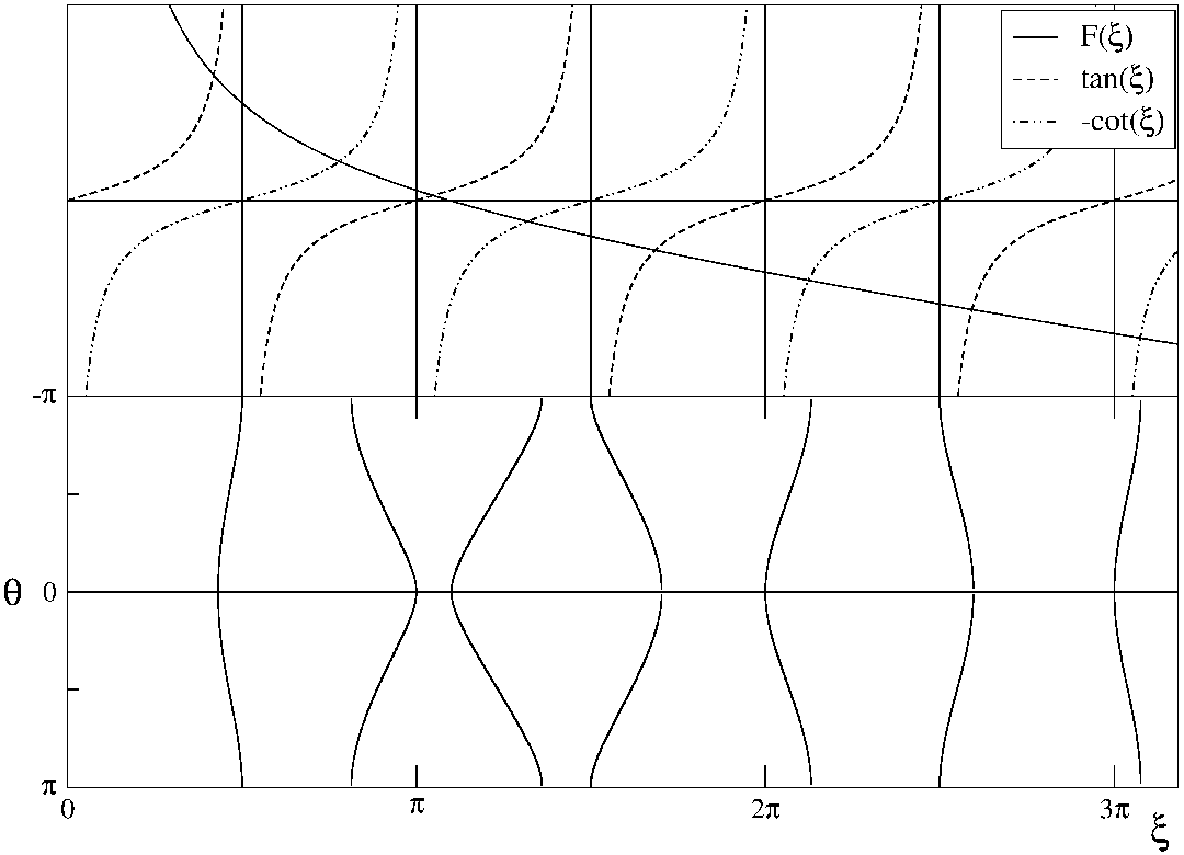
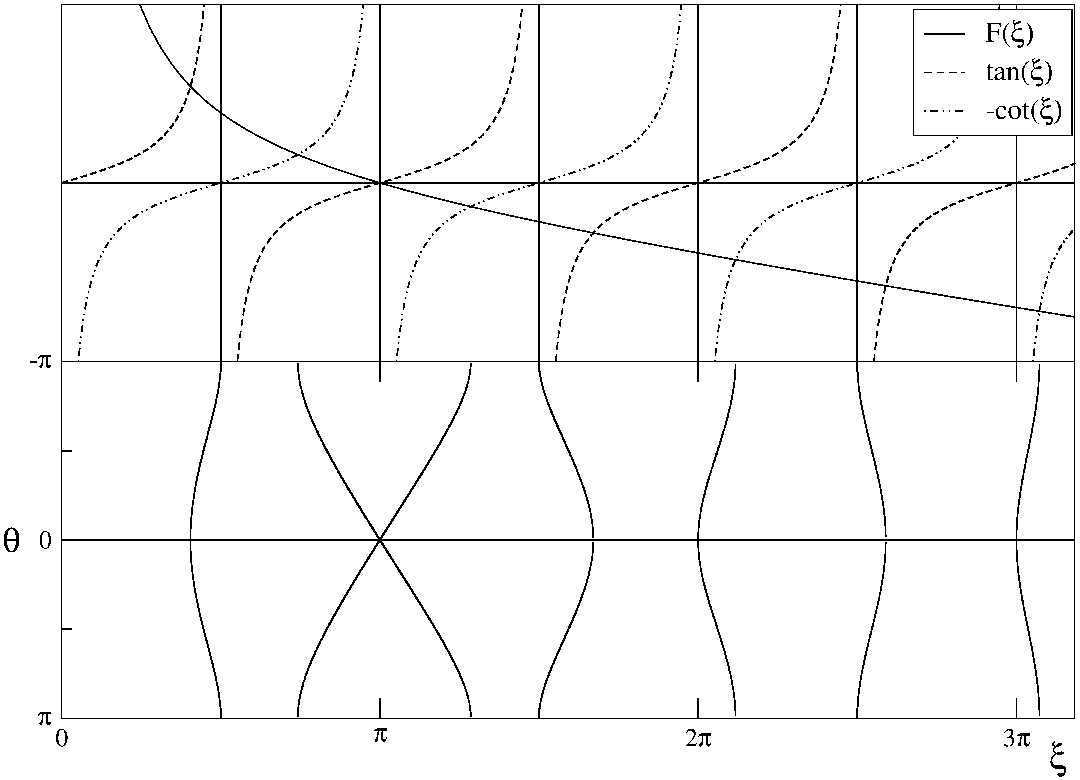
Graphic solutions of the transcendental equations (3.55) and (3.56) are given in the upper part of figures 1(a) and 1(b). The chain of inequalities (3.49) follows by the monotone behavior of F⁡(ξ)F(\xi).

Degeneration of eigenvalues for ωo/ωg=n/2\omega_{o}/\omega_{g}=n/2, the fact that −E⁡(θ)-E(\theta) is an eigenvalue if E⁡(θ)E(\theta) is an eigenvalue and relation (3.50) follow directly by equation (3.41) and by F⁡(ξ)=−F⁡(−ξ)F(\xi)=-F(-\xi). ∎

Refer to caption
(a) With non degenerate eigenvalues. M/Mg=0.5M/M_{g}=0.5, ωo/ωg=1.2\omega_{o}/\omega_{g}=1.2
Refer to caption
(b) With one degenerate eigenvalue. M/Mg=0.5M/M_{g}=0.5, ωo/ωg=1\omega_{o}/\omega_{g}=1
Figure 1: The upper part of figures shows the graphical solution of equations (3.55) and (3.56). The lower part shows the band structure.

One can show that there is a band structure writing equation (3.41) as

tan2⁡θ​L2=tan⁡ξ⁡[tan⁡ξ−F⁡(ξ)1+F⁡(ξ)​tan⁡ξ]\tan^{2}\frac{\theta L}{2}=\tan{\xi}\left[\frac{\tan\xi-F(\xi)}{1+F(\xi)\tan\xi}\right] (3.57)

It is possible to find solutions of equation (3.57) only for values of ξ\xi such that the r.h.s. is positive. In the lower part of figures 1(b) and 1(a) the resulting band structure is shown. The figures clearly show that the width of the gaps is connected to the structure of the spectrum. In particular figure 1(b) shows that when there is a degenerate eigenvalue, ωo/ωg=n​π/2\omega_{o}/\omega_{g}=n\pi/2 with n∈ℕn\in\mathbb{N}, a gap disappears because of the overlapping of two bands.

The bandwidth increases, when the ratio M/MgM/M_{g} decreases.

References

  • [AGH-KH] S. Albeverio, F. Gesztesy, R. Høegh-Krohn, H. Holden, Solvable Models in Quantum Mechanics: second edition, AMS Chelsea Publ. (2005).
  • [D] P.A.M. Dirac, Classical Theory of Radiating Electrons, Proc. R. Soc. London, Ser. A, 167, 148-169 (1938).
  • [GG] V.I. Gorbachuk, M.L. Gorbachuk, Boundary Value Problems for Operator Differential Equations, Kluwer Acad. Publ. (1991).
  • [GS] D.J. Griffiths, C.A. Steinke, Waves in Locally Periodic Media, Am. J. Phys., 69, No. 2, 137-154 (2001).
  • [IW] L. Infeld, P.R. Wallace, The Equation of Motion in Electrodynamics, Phys. Rev., 57, 797-806 (1940).
  • [K] J. Kijowski, Electrodynamics of Moving Particles, Gen. Rel. Grav., 26, 167-201 (1994).
  • [M] M. Marino, Classical Electrodynamics of Point Charges, Ann. Phys., 301, 85-127 (2002).
  • [NP1] D. Noja, A. Posilicano, The Wave Equation with One Point Interaction and the (Linearized) Classical Electrodynamics of a Point Particle, Ann. Inst. Henri Poincaré, 68, 351-377 (1998).
  • [NP2] D. Noja, A. Posilicano, On the Point Limit of the Pauli-Fierz Model, Ann. Inst. Henri Poincaré, 71, 425-457 (1999).
  • [P1] A. Posilicano, A Kreĭn-like Formula for Singular Perturbations of Self-Adjoint Operators and Applications, J. Funct. Anal., 183, 109-147 (2001).
  • [P2] A. Posilicano, Singular Perturbations of Abstract Wave Equations, J. Funct. Anal. (at press)
  • [RS1] M. Reed, B. Simon, Methods of Modern Mathematical Physics. Vol 1: Functional Analysis, Academic Press (1972).
  • [RS2] M. Reed, B. Simon, Methods of Modern Mathematical Physics. Vol 2: Fourier Analysis, Self-Adjointness, Academic Press (1975).
  • [RS3] M. Reed, B. Simon, Methods of Modern Mathematical Physics. Vol 3: Scattering Theory, Academic Press (1979).
  • [RS4] M. Reed, B. Simon, Methods of Modern Mathematical Physics. Vol 4: Analysis of Operators, Academic Press (1978).
  • [SW1] A. Soffer, M.I. Weinstein, Nonautonomous Hamiltonians, J. Stat. Phys., 93, No. 1-2, 359-391 (1998).
  • [SW2] A. Soffer, M.I. Weinstein, Time Dependent Resonances Theory, Geom. Funct. Anal., 8, 1-43 (1998).
  • [SW3] A. Soffer, M.I. Weinstein, Resonances, Radiation Damping and Instability in Hamiltonian Nonlinear Wave Equations, Invent. Math., 136, 9-74 (1999).
  • [S] H. Spohn, Dynamics of Charged Particles and their Radiation Field, Cambridge Univ. Press (2004).
  • [T] J.D. Templin, Radiation Reaction and Runaway Solutions in Acoustics, Am. J. Phys., 67, No. 5, 407-413 (1999).