Multiple Schramm-Loewner Evolutions
and
Statistical Mechanics Martingales
Abstract
A statistical mechanics argument relating partition functions to martingales is used to get a condition under which random geometric processes can describe interfaces in 2d statistical mechanics at criticality. Requiring multiple SLEs to satisfy this condition leads to some natural processes, which we study in this note. We give examples of such multiple SLEs and discuss how a choice of conformal block is related to geometric configuration of the interfaces and what is the physical meaning of mixed conformal blocks. We illustrate the general ideas on concrete computations, with applications to percolation and the Ising model.
Michel Bauer a, Denis Bernard a 11 1 Member of C.N.R.S, Kalle Kytölä b
michel.bauer@cea.fr; denis.bernard@cea.fr; kalle.kytola@helsinki.fi
a Service de Physique Théorique de Saclay
CEA/DSM/SPhT, Unité de recherche associée au CNRS
CEA-Saclay, 91191 Gif-sur-Yvette, France.
b Department of Mathematics, P.O. Box 68
FIN-00014 University of Helsinki, Finland.
1 Introduction
Growth phenomena are ubiquitous around us. They have both very practical applications and theoretical relevance. But they are rarely easy to study analytically and very few rigorous or exact results are known. In two dimensions, the description of a growing domain is often obtained indirectly through the description of a family of univalent holomorphic representations, leading quite generally to equations known under the name of Loewner chains. These techniques, based on the Riemann mapping theorem, are conceptually important but usually far from making the problem tractable.
In the last few years, Loewner chains have been discovered which have a large hidden symmetry – conformal invariance – that makes them more amenable to an exact treatment [1]. These are known under the name of Stochastic or (Schramm) Loewner evolutions SLE.
Their mathematical elegance and simplicity is not their sole virtue. They are also natural candidates to describe the continuum limit of an interface in two-dimensional statistical mechanics models at criticality. At the critical temperature and in the continuum limit, the system is believed to be conformally invariant and physicists have developed many powerful techniques, known under the name conformal field theory or CFT, to deal with local questions in a conformally invariant 2d system. However, nonlocal objects like interfaces posed new nontrivial problems that finally SLE could attack in a systematic way [5, 4]. The connection between CFT and SLE is now well understood [8, 7, 9, 11, 12, 14] and the interplay between the two approaches has proved fruitful.
The way SLE describes an interface deserves some comments. As a guiding example, consider the Ising model in a simply connected domain, say on the hexagonal lattice. Suppose that the boundary is split in two arcs with endpoints say and and impose that on one arc the spins are up and on the other one the spins are down. In this situation each sample exhibits an interface. It joins the two points where the boundary conditions change and splits the domain in two pieces, one with all spins up on its boundary and one with all spins down. This interface fluctuates from sample to sample. What SLE teaches us is the following. Instead of describing the interface between and at once, SLE views it as a curve starting from say and growing toward . And SLE describes the distribution for the addition of an infinitesimal piece of interface when the beginning of the interface is already known. So the description is in terms of a growth process even if there was no growth process to start with.
As mentioned above, the probabilistic aspects of SLE as well as its connections with conformal field theory are now fairly well understood. However, some fundamental questions remain, again directly related to natural questions in the statistical mechanics framework.
The one we shall concentrate on in this note is what happens when, due to boundary conditions, the system contains several interfaces. Proposals for multiple SLEs have already been made in the literature [15, 16], but our results point to a different picture. The simplest situation is in fact when there is only one interface but we want to deal with its two ends symmetrically so that two growth processes will interact with each other. Remember that standard SLE deals with the two ends of the interface asymmetrically. This has a price : time reversed SLE is an intricate object.
As a guiding example for more than one interface, consider again the Ising model in a simply connected domain on the hexagonal lattice. If one changes boundary conditions from up to down to up and so on times along the boundary, each sample will exhibit interfaces, starting and ending on the boundary at points where the boundary conditions change, forming a so-called arch system. However, the interfaces will fluctuate from sample to sample and so does even the topology of the arch system. This topology, for instance, is an observable that is trivial for a single SLE.
Our description will again be in terms of growth processes and Loewner chains. For standard SLE, the driving parameter is a continuous martingale and the tip of the curve separates two different states of the system (up and down spins for Ising), leading to a well defined boundary changing operator in statistical mechanics. The relation between the stochastic Loewner equation and the boundary changing operator comes via a diffusion equation that they share in common.
For multiple SLEs, we expect that for short time scales each curve grows under the influence of an independent martingale. At its tip stands the same boundary changing operator. But we also expect drift terms, describing interactions between the curves.
The possibility of different arch topologies makes it even more natural to have a description with one curve growing at each boundary changing point so that each of them is on the same footing. So interfaces are described by growth processes of “half-interfaces” that finally pair in a consistent way to build arches.
In statistical mechanics, each arch system has a well defined probability to show up. The law governing this finite probability space is again described by a Boltzmann weight which is nothing but a partial partition function.
Our starting point is the reconsideration of the role of Boltzmann weights and partition functions in statistical mechanics and their simple but crucial relationship with probabilistic martingales. This allows us to ask the question “by what kind of stochastic differential equations can one describe multiple SLEs ?” by imposing a martingale property and conformal invariance. This puts strong constraints on the drift terms and our main result is a description of the family of drift terms that are compatible with the basic rules of statistical mechanics. Each drift is expressed in terms of the partition function of the system. This partition function is given by a sum of Boltzmann weights for configurations that satisfy certain boundary conditions : at the starting points of the curves the boundary conditions change. The partition function depends on the position of these changes, so up to normalization, the partition function is in fact a correlation function. It satisfies a number of partial differential equations (one equation for each point) that are related to the diffusion equations for the multi SLE process. The solutions form a finite dimensional vector space. The positivity constraint satisfied by physical partition functions singles out a cone which is expected, again guided by statistical mechanics, to have the same dimension of the underlying vector space and to be the convex hull of a family of half lines, so that a generic hyperplane section of the cone is a simplex.
So geometrically, the drift terms are parametrized by a cone. Extremal drifts, i.e. drifts corresponding to extremal lines in this cone, lead to processes for which the final pattern formed by the growing curves is a given arch system. Drifts inside the simplex give rise to stochastic processes where the asymptotic arch system fluctuates from sample to sample. A crucial role to construct martingales describing interesting events is played by the short distance expansion in conformal field theory because this is what tells which terms in the partition function become dominant when an arch closes, i.e. when two driving processes of the multi SLE hit each other.
The vector space of solution of the differential equations for the partition functions has a famous basis indexed by Dyck paths, which are in one to one correspondence with arch systems. But the basis elements do not in general correspond to extremal partition functions. We shall give a rationale for computing the matrix elements for the change of basis and compute a number of them, but we have no closed general formula.
We shall illustrate our proposal with concrete computations for to interfaces with applications to percolation and the Ising model. We shall also discuss the classical (deterministic) limit , where only extremal drifts survive.
The notes also cover the case when a number of boundary changes are very close to each other but the system is conditioned so that they do not pair with each other. The details are in the main text.
Our description is rather flexible in the sense that the speed of growth of each piece of interface can be tuned. Certain limiting cases lead to previously known processes which are examples of SLE processes.
It is appropriate here to stress that many of the probabilistic properties of the solutions of the stochastic differential equations that we introduce are conjectural at this point. We have made some consistency checks22 2 For instance, Dubédat has derived general “commutation criteria” [16] for multiple SLEs. The processes we study are a special class satisfying commutation. This class extends vastly the special solution found by Dubédat, which in our language corresponds to self avoiding SLEs moving to infinity. and the whole pattern is elegant, but our confidence comes more from our familiarity with conformal field theory and statistical mechanics.
2 Basics of Schramm-Löwner evolutions: Chordal SLE
Let us briefly recall what is meant by the chordal SLE — detailed studies can be found in [2] or [3]. The chordal SLE process in the upper half plane is defined by the ordinary differential equation
| (1) |
where the initial condition is and is a Brownian motion with variance parameter . Let denote the explosion time of (1) with initial condition and define the hull at time by . Then is a family of growing hulls, for . The complement is simply connected and is the unique conformal mapping with at . One defines the SLE trace by . The trace is a continuous path in and it generates the hulls in the sense that is the unbounded component of . For the trace is a non-self-intersecting path and it doesn’t hit for so . For a typical point is swallowed, i.e. for large but . In the parameter range the trace is space filling, . Let us point out that no statistical mechanics models seem to correspond to .
In the definition of chordal SLE we took the usual parametrization of time. From equation (1) we see that , which means (this could be taken as a definition) that the capacity of from infinity is . Since the capacity goes to infinity as , the hulls are not contained in any bounded subset of .
If the parametrization of time is left arbitrary, Schramm’s argument yields :
where is a continuous martingale with quadratic variation (an increasing function going to infinity with ). In this formula, both and are random objects. The capacity of is . But this is not really more general than eq.(1) which is recovered by a random time change.
3 A proposal for multiple SLEs
The motivations for our proposal require a good amount of background, but the proposal and its main features themselves can be easily stated. We gather them in this section. Some of the results are conjectures. The rest of the paper will then be split into sections whose purpose will be either to motivate our proposal in general, or to prove its correctness in certain special but nontrivial cases by explicit computations.
3.1 The basic equations
We propose to describe the local growth of interfaces in CFT, labeled by an integer and joining fixed points on the boundary by a Loewner chain. We assume that in the following. We list the set of necessary conditions and equations.
Conformal invariance: The measure on SLE is conformally invariant. Hence it is enough to give its definition when the domain is the upper half plane in the hydrodynamical normalization.
Universe: The basic probabilistic objects are (continuous, local) martingales , with quadratic variation absolutely continuous with respect to and vanishing cross variation, defined on an appropriate probability space. By a time change we can and shall assume that .
Driving processes: The processes are solutions of the stochastic differential equations
| (2) |
The initial conditions are ordered in such a way that .
Loewner chain: The map uniformizing the complement of the hulls satisfies
| (3) |
The initial condition is . With our conventions, the total capacity of the growing hulls at time is .
Auxiliary function: The system depends on a function which has to fulfill the following requirements :
is defined and positive for ,
is translation invariant and homogeneous. Its weight is for some nonnegative integer , where33 3 A more traditional notation for is in the physics literature.
is annihilated by the differential operators
We call this system of equations the SLE system for curves joining together the points and possibly the point at infinity. Systems for radial and dipolar versions of SLE could be defined analogously.
3.2 Arch probabilities
It is known from CFT that (relaxing the positivity constraint), the solutions to form a vector space of dimension .
The positive solutions form a cone and from the statistical mechanics interpretation, we conjecture that this cone has the same dimension and is generated by (i.e. is the convex hull of) half lines (extremal lines, pure states in the sense of statistical mechanics) so that a transverse section of the cone is a simplex. So each solution can be written in a unique way as a sum of extremal states.
The numbers have many many combinatorial interpretations, but the one relevant for us is the following. Draw points ordered cyclically on the (extended) real line bounding the upper half plane . Consider disjoint curves in such that each is an end point of exactly curve and is an end point of exactly curves. There are topologically inequivalent configurations, called arch configurations when . We keep the same name for , writing archm configurations when precision is needed.
Motivated by this, we claim the following :
a) To each arch configuration corresponds an extremal state in the following sense : the solution of the SLE system with can be defined up to a (possibly infinite) time, at which the growing curves have either paired together or joined the point at infinity and at that time the topology is that of the arch with probability one.
b) One can decompose a general solution of as a sum of
c) The probability that a solution of the SLE system with auxiliary function ends in arch configuration is the ratio
evaluated at the initial condition .
The first step toward a heuristic derivation of the above results will be to explain how to construct martingales – in particular martingales associated to interfaces – from statistical mechanics observables in a systematic way. But we start with a few comments.
4 First comments
4.1 Statistical mechanics interpretation
To have a specific example in mind, think again of the Ising model at the critical temperature. Let be the lattice spacing.
First, put changes of boundary conditions from spins up to spins down and so on along the boundary at points . In the continuum limit when but have a finite limit, the partition function behaves like a homogeneous function of weight (when both and the ’s are rescaled) and CFT teaches us that satisfies for . Then, if is an arch system, should be (proportional to the continuum limit of) the partial partition function when the sum of Boltzmann weights is performed only over the interface configurations with topology .
To make generalized arch configurations, choose and with . Put changes of boundary conditions from spins up to spins down and so on along the boundary, at points and at . Sum only over configurations where the interfaces do not joint two -type points to each other. Take the continuum limit for the ’s as before, but impose that all ’s go to infinity and remain at a finite number of lattice spacings from each other. This is expected to lead again to a partition function of weight (when both and the ’s are rescaled) and satisfies for the given and . If is an archm configuration, should be (proportional to the continuum limit of) the partial partition function when the sum of Boltzmann weights is performed only over the interface configurations with topology .
Note that the prefactor between the continuum limit finite part and the real partition function is a power of the lattice spacing. The power depends on , so it is likely to be unphysical to use a non homogeneous in the SLE system, mixing different values of for a fixed . However, we shall later treat the example mixing and because it is illustrative despite the fact that it breaks scale invariance.
4.2 SLE as a special case of SLE
For the solution of with is elementary. Writing and , one finds . Taking the first martingale to be a Brownian and the second one to be , one retrieves the equations for SLE growing from point to point in the hydrodynamical normalization. Let us recall briefly why.
We start from SLE from to . The basic principle of conformal invariance makes the passage from this special case to the case when SLE goes from point to point on a routine task. If is any linear fractional transformation (i.e. any conformal transformation) from to itself mapping to and to , the image of the SLE trace or hull from to by is by definition an SLE trace from to and this is measure preserving. The new uniformizing map is and it is readily checked that is a rational function of whose precise form can be easily computed but does not concern us.
Let us just mention that this rational function is regular everywhere (infinity included) except for a simple pole at and has a third order zero at . So the map is normalized in such a way that , which is not the hydrodynamic normalization.
But if is any linear fractional transformation, describes the same trace as . As long as the trace does not separate from , i.e. as long as the trace has not hit the real axis in the segment , i.e. as long as is not in the hull, can be adjusted in such a way that is normalized hydrodynamically. Then is a function of which is regular everywhere but for a single pole and vanishes at infinity, i.e. one can write . The following computation is typical of the manipulations made with SLE (see e.g. [4]). Write an compute from the definition
Comparison gives
But is regular at from which one infers that (the poles in the two terms are at the same point) and (the two residues add to ). Going one step further in the expansion close to yields Ito’s formula gives So the time change together with the definition yields
But because is a linear fractional transformation. Finally, setting , and we can summarize
where is a Brownian motion with quadratic variation , , , . Thus chordal SLE from to in the hydrodynamical normalization is indeed a special case of SLE.
The above equations are also a special case of SLE , but it should be clear that our general proposal goes in a different direction.
As already mentioned, the description of chordal SLE from to in the hydrodynamical normalization in fact coincides with chordal SLE from to only up to the first time is separated from by the trace. This time is infinite for , but it is finite with probability for . The most obvious case is . The equation is nothing but the usual chordal SLE6 ending at infinity, a consequence of locality (in the SLE sense, not in the quantum field theory sense used later). At that time, the real chordal SLE from to swallows , whereas the hydrodynamically normalized version swallows . The solution to this problem is to use conformal invariance and restart the process again in the correct domain at the time when and get separated by the trace. But this is not coded in the equations.
4.3 Making sense
The previous example should serve as a warning. Some serious mathematical work may have to be done even to make sense of our conjectures, let alone prove their correctness. The problems might be of different natures for and . We content with the following naive remarks. One of the problems is that the arches do not have to close at the same time. It may even happen that one of the growing curves touches the real line or another curve in such a way that the upper half plane is split in two domains and the one which is swallowed contains some of the growing curves.
Our putative description of SLE processes can be valid in this form only up the realization of such an event. The first thing to check should be that the event is realized with a probability obtained by summing over all ’s corresponding to compatible configurations (see figure 1). In particular, the connected component of should contain at least curves for consistency, but that’s not an obvious property of our proposal.

Consider the fate of the connected component of . If is even, conformal invariance suggests to continue the Loewner evolution simply by suppressing the points that have been swallowed, i.e. for the remaining points. If is odd, the same should be done, but the image of the point at which one interface has made a bridge should be included as a starting point for the continuation of the evolution. Preferably, the function for this new SLE system should not be adjusted by hand to make our conjectures correct, but should appear as a natural limit. We shall make comments on this and give concrete illustrations later.
For the component that is swallowed, one can use conformal invariance again to change the normalization of the Loewner map in such a way that this component is the one that survives and then restart a new SLE for the appropriate number of points. This procedure may have to be iterated.
Note also that our conjectures for arch probabilities do not involve any details on the martingales . Indeed, we expect that there is some robustness. But the precise criteria are beyond our understanding.
4.4 A few martingales for SLEs
Our heuristic derivation of the SLE system will in particular show that if also solves (even relaxing positivity), the quotient
is a local martingale. This can be proved directly using Ito’s formula.
In particular,
is a local martingale bounded by , hence a martingale. On the other hand, a standard argument shows that if is the probability that the system ends in a definite arch configuration (once one has been able to make sense of it) is a martingale. This is an encouraging sign. To get a full proof, one would need to analyze the behavior of when one arch closes, or when one growing curve cuts the system in two, to get recursively a formula that looks heuristically like
if the system forms asymptotically the arch system at large . Such a formula rests on properties of when some points come close together in a way reminiscent to the formation of arch : should dominate all ’s, in such circumstances. In section 8 we shall use this to expand explicitly the ’s in a basis of solutions to which is familiar from CFT, very explicitly at least for small .
4.5 Classical limit
Our proposal for SLE has a non trivial classical limit at . The martingales vanish in this limit, but the remain arbitrary increasing functions. The function does not have a limit, but the do. They are kind of Ricatti variables for which the equations read
which have a limit when , comparable to the classical limit of a Schroedinger equation. To summarize, the classical limit is
where the auxiliary functions are homogeneous functions of degree which satisfy and
It is not too surprising that the differential equations for have become algebraic equations for the ’s, so that the space of solutions which was a connected manifold for concentrates on a finite number of points in the classical limit. The classical system, maybe with an educated guess for the ’s, could be interesting for its own sake.
4.6 Relations with other work
Several processes involving several growing curves have appeared in the literature.
The first proposal was made by Cardy [15]. It can be formally obtained from ours by forgetting the conditions and choosing a constant . The corresponding processes are interesting, but the relationship with interfaces in statistical mechanics and CFT is unclear for us.
Dubédat [16] has derived a general criterion he calls commutativity to constrain the class of processes that could possibly be related to interfaces. Our proposal satisfies commutativity so they can be viewed as a special case satisfying other relevant physical constraints. Dubédat also came with a special solution of commutativity. It corresponds to the case in our language. Then the space of solutions has dimension and the corresponding partition function is elementary:
| (4) |

A single arch topology is possible, all interfaces converge to , see figure 2. Maybe this is a good reason to call this case chordal SLE.
5 CFT background
There was never any doubt that SLEs are related to conformal field theories. The original approach [7, 12, 11, 14] used the operator formalism because if yields naturally martingale generating functions. Here, we use the correlator approach for a change. We restrict the presentation to a bare minimum, referring the newcomer to the many articles, reviews and books on the subject ([18, 17]). The reader who knows too little or too much about CFT can profitably skip this section.
Observables in CFT can be classified according to their behavior under conformal maps. Local observables in quantum field theory are called fields. For instance, in the Ising model, on an arbitrary (discrete) domain, the average value of a product of spins on different (well separated) sites can be considered. Taking the continuum limit at the critical point, we expect that on arbitrary domains there is a local observable, the spin. The product of two spins at nearest neighbor points corresponds to the energy operator. In the continuum limit, this will also lead to a local operator. In this limit, the lattice spacing has disappeared and one can expect a definite (but nontrivial) relationship between the energy operator and the product of two spin fields close to each other. As on the lattice the product of two spins at the same point is , we can expect that the identity observable also appears in such a product at short distances. Local fields come in two types, bulk fields whose argument runs over and boundary fields whose argument runs over . In this paper, we shall not need bulk fields so we leave them aside.
The simplest conformal transformations in the upper-half plane are real dilatations and boundary fields can be classified accordingly. It is customary to write to indicate that in a real dilatation by a factor the field picks a factor . By a locality argument, boundary fields in a general domain (not invariant under dilatations) can still be classified by the same quantum number. The number is called the conformal weight of .
There are interesting situations in which (due to degeneracies) the action of dilatations cannot be diagonalized, leading to so called logarithmic CFT. While this more general setting is likely to be relevant for several aspects of SLE, we shall not need it in what follows.
Under general conformal transformations, the simplest objects in CFT are so called primary fields. Their behavior is dictated by the simplest generalization of what happens under dilatations. Suppose are boundary primary fields of weights . If is a conformal map from domain to a domain , CFT postulates that
Symbolically, this can be written . It is interesting to make a comparison of these axioms with the previous computations relating chordal SLE from to to chordal SLE from to in several normalizations. This also involved pure kinematics.
As usual in quantum field theory, to a symmetry corresponds an observable implementing it. In CFT, this leads to the stress tensor whose conservation equation reduces to holomorphicity. The fact that conformal transformations are pure kinematics translates into the fact that insertions of in known correlation functions can be carried automatically, at least recursively. The behavior of under conformal transformations can be written as where is the Schwarzian derivative and is a conformal anomaly, a number which is the most important numerical characteristic of a CFT. When , is be a primary field i.e. an holomorphic quadratic differential. When a (smooth) boundary is present, the Schwarz reflection principle allows to extend by holomorphicity. Holomorphicity also implies that if is any local (bulk or boundary) observable at point and is vector field meromorphic close to , the contour integral along an infinitesimal contour around oriented counterclockwise is again a local field at , corresponding to the infinitesimal variation of under the map . It is customary to write for . It is one of the postulates of CFT that all local fields can be obtained as descendants of primaries, i.e. by applying this construction recursively starting from primaries. The correlation functions of descendant fields are obtained in a routine way from correlations of the primaries. But descendant fields do not transform homogeneously.
When is holomorphic at , is a familiar object. For instance, if is a primary boundary field, one checks readily that for , and . The other descendants are in general more involved, but by definition the stress tensor is the simplest descendant of the identity . It does indeed not transform homogeneously.
A primary field and its descendants form what is called a conformal family. Not all linear combinations of primaries and descendants need to be independent. The simplest example is the identity observable, which is primary with weight and whose derivative along the boundary vanishes identically44 4 For other primary fields with the same weight if any, this does not have to be true.. By contour deformation, this leads to translation invariance of correlation functions when has translation symmetry.
The next example in order of complexity is of utmost importance for the rest of this paper. If , the field
is again a primary, i.e. it transforms homogeneously under conformal maps. In this case, consistent CFTs can be constructed for which it vanishes identically. This puts further constraints on correlators.
For example, when is the upper half plane, so that the Schwarz principle extends to the full plane, the contour for can be deformed and shrunken at infinity. Then, for an arbitrary boundary primary correlator one has
| (5) | |||||
It is customary to call this type of equation a null-vector equation.
Note that the primary field of weight sitting at has led to no contribution in this differential equation. Working the other way round, this equation valid for an arbitrary number of boundary primary fields with arbitrary weights characterizes the field and the relation between and the central charge .
The case of three points correlators is instructive. Global conformal invariance implies that
The proportionality constant might depend on the cyclic ordering of the three points. But if the differential equation for is used, a further constraint appears. The three point function can be non vanishing only if
This computation has a dual interpretation : consider a correlation function with any number of fields, among them a and a . If and come very close to each other they can be replaced by an expansion in terms of local fields. This is called fusion. Several conformal families can appear in such an expansion, but within a conformal family, the most singular contribution is always from a primary. This argument applies even if and are arbitrary. But suppose they are related as above and the differential equation eq.(5) is valid. This equation is singular at and at leading order the dominant balance leads to an equation where the other points are spectators. One finds that the only conformal families that can appear are the ones whose conformal weight satisfies the fusion rule.
This is enough CFT background for the rest of this paper. We are now in position to give the heuristic argument that leads to our main claims.
6 Martingales from statistical mechanics
The purpose of this section is to emphasize the intimate connection between the basic rules of statistical mechanics and martingales. The connection is somehow tautological, because statistical mechanics works with partition functions, i.e. unnormalized probability distributions, all the time. In the discrete setting, this makes conditional expectations a totally transparent operation that one performs without thinking and even without giving it a name. But the following argument is, despite its simplicity and its abstract nonsense flavor, the crucial observation that allows us to relate interfaces in conformally invariant statistical mechanics to SLEs.
6.1 Tautological martingales
Consider a model of statistical mechanics with a finite but arbitrarily large set of possible states . Usually one starts with models defined on finite grid domains so is natural. To each state we associate a Boltzmann weight55 5 Usually the Boltzmann weight is related to the energy of the state through , where is the inverse temperature (a Lagrangian multiplier related to temperature, anyway). . The partition function is so that it normalizes the Boltzmann weights to probabilities, . Since is finite, we can use the power set as a sigma algebra. The expected value of a random variable is denoted by .
Note that if is a collection of disjoint subsets of such that , then the collection of all unions is a sigma algebra on . Conversely, since is finite, any sigma algebra on is of this type.
Consider a filtration, that is an increasing family of sigma algebras for all . Denote the corresponding collections of disjoint sets by and define the partial partition function . The conditional expectation values
are martingales by definition: for we have
Notice that the probability of the event is conveniently .
Suppose that the model is defined in a domain and that there are interfaces in the model. Parametrize portions of these interfaces touching the boundary by an arbitrary “time” parameter in such a way that paths , (which are pieces of the random interfaces) emerge from the boundary at and are disjoint at least when is small enough, see figure 3. To avoid confusion we write the time parameter now as a subscript and continue to indicate the dependence of by parenthesis, so is a parametrization of the piece of interface if the system is at state . Then we can consider the natural filtration of the interface by taking to be the sigma algebra generated by the random variables up to time .

The boundary conditions of the model are often such that conditioning on the , is the same as considering the model in a smaller domain (a part of the interface removed) but with same type of boundary conditions. Of course the position at which the new interface should start is where the original interface would have continued, that is the ’s. Let be the domain with the removed.
The starting point of the next section is the input of conformal invariance in this setup.
6.2 Simplifying tautological martingales
We start from the situation and notations at the end of the previous section. If in addition we are considering a model at its critical point, then the continuum limit may be described by a conformal field theory. At least for a wide class of natural observables , the expectation values become CFT correlation functions in the domain of the model
We need to write the correlation function of identity (proportional to ) in the denominator because the boundary conditions (b.c.) of the model may already have led to insertions of boundary changing operators that we have not mentioned explicitly.
The closed martingales become
where in the continuum limit might be with hulls (and not only traces) removed.
For certain (but not all) observables, is computing a probability, which in a conformal field theory ought to be conformally invariant. But is written as a quotient, and this means that the numerator and denominator should transform homogeneously (and with the same factor) under conformal transformations. In particular, the denominator should transform homogeneously. This means that – which depends on the position of the boundary condition changes – behaves like a product of boundary primary fields. Then, by locality, for any , the transformation of the numerator under conformal maps will split in two pieces: one containing the transformations of and the other one canceling with the factor in the denominator. So we infer the existence in the CFT of a primary boundary field, denoted by in what follows, which implements boundary condition changes at which interfaces anchor. Hence we may write
and
As will become clear later, there might also be one further boundary operator anchoring several interfaces. We do not mention it explicitly here because it will sit at a point which will not be affected by the conformal transformations that we use.
Write the transformation of the observable as under a conformal map. Denote by a conformal representation and write . The expression for the closed martingale can now be simplified further
| (6) |
The Jacobians coming from the transformations of the boundary changing primary field have canceled in the numerator and denominator. The explicit value of the conformal weight of does not appear in this formula.
Of course, we have cheated. For the actual map which is singular at the ’s these Jacobians are infinite. A more proper “derivation” would go through a regularization but locality should ensure that the naive formula remains valid when the regularization is removed. Eq.(6) is the starting point of our analysis.
7 Derivation of the proposal
The heuristics we follow is to describe a growth process of interfaces by a Loewner chain compatible with conformal invariance in that the right hand side of eq.(6) is a martingale.
7.1 The three ingredients
Loewner chain: If we use the upper half plane as a domain, , and impose the hydrodynamic normalization, the equation for has to be of the form
for some processes , . The initial condition is .
Interfaces grow independently of each other on very short time scales: Schramm’s argument deals with the case of a single point. We expect that on very short time scales the growth processes do not feel each other and Schramm’s argument is still valid, so that where the ’s are (continuous,local) martingales with quadratic variation and vanishing cross variation and is a drift term.
The martingale property fixes the drift term: The drift term will be computed by imposing the martingale condition on when is a product of an arbitrary number of boundary primary fields . The insertion points are away from the boundary changing operators and is regular with positive derivative there. Substitution of in formula (6) yields
| (7) |
7.2 Computation of the Ito derivative of
In formula (7), denote respectively by , and the numerator, denominator and Jacobian factor on the right hand side.
It is useful to break the computation of in several steps.
– Preliminaries.
Ito’s formula for the ’s gives
Using the Loewner chain for and its derivative with respect to , one checks that
– The Ito derivative of .
The time being given, we can simplify the notation. Set and and apply the
chain rule to get
– First use of the null-vector equation : identification
of .
Let us concentrate for a moment on the familiar chordal SLE case, for
which . The drift term is known to be zero. The
boundary conditions also change at (the endpoint of the
interface) and there is an operator there, that we have not written
explicitly because the notation is heavy enough. Anyway, is a
two-point function with one of the fields at infinity, so it is a
constant. For chordal SLE, the drift term in the Ito derivative of the
putative martingale vanishes if and only if
where for simplicity we have written .
Comparison with eq.(5) implies that has a vanishing
descendant at level two and has conformal weight
:
The central charge is
.
This is of course nothing but the correlation function formalism
version of the original argument relating SLE to CFT, which was given
in the operator formalism, see [7].
– Second use of the null-vector equation.
Now that has been identified, we can return to the general
case, with an arbitrary number of growing curves. Each growing
curve has its own field and each field comes with its
differential equation, which is eq.(5) but for
spectator fields, the fields and the other
’s. So is annihilated by the differential
operators
We can use this to get a simplified formula
where is the first order differential operator
The formula for is just the special case .
– Final application of Ito’s formula.
where is the first order differential operator
The martingale property is satisfied if and only if the drift terms vanish.
7.3 Main claim
To summarize, we have shown that the system
admits conditioned correlation functions from CFT as martingales if and only if
where is a partition function. It is under this condition that it describes the growth of interfaces in a way compatible with statistical mechanics and conformal field theory.
In fact, we have used a special family of correlators. But the same argument applies to all operators (hence the “if” part). Of special interest in the sequel will be the case when is a topological observable, for instance taking value if the interface forms a given arch system and otherwise. No Jacobian is involved for such observables and the numerator looks again like a partition function.
7.4 The moduli space
From the definition of as a correlation of primary fields with null descendants at level , it is clear that properties are satisfied, except maybe for the quantization of the possible scaling dimensions of , to which we turn now.
This is standard material from CFT and we include it here for completeness.
The correlator on the real line satisfies differential equations. We shall recall why the space of simultaneous solutions which have global conformal invariance has dimension
if for some nonnegative integer and has dimension otherwise. This will end the derivation of our proposal and match the counting of arches.
At the end of the background on conformal invariance, we mentioned fusion rules: when and a are brought close together, they can be expanded in a basis of local operators that can be grouped in conformal families. We also recalled why the weight of the primaries in each conformal family had to satisfy so that only two conformal families can appear in a fusion with . The two conformal weights are easily found to be . Furthermore, and one can show that the corresponding field has to be the boundary identity operator. By global conformal invariance, the only local operator with a non vanishing one point correlator is the identity and boundary two point functions vanish unless the two local fields have the same conformal weight. This takes care of the counting and selection rules for the cases.
One proceeds by recursion. The points are ordered . If then move close the (for instance by a global conformal transformation) and fuse to get an expansion for local fields at say. Only the conformal families of appear. If this fixes the weight of the field at . If , iterate. This leads immediately to the selection rules mentioned above : the field at infinity has to be a . The dimension is nothing but the number of path of steps from to on the nonnegative integers, a standard combinatorial problem whose answer is . The efficient way to do the counting is by the reflection principle. The possible outcomes of each fusion can be encoded in a so-called Bratelli diagram:
| (8) |
This is totally parallel to the discussion of composition of spins for the representation theory of the Lie algebra of rotations. The multiplicity is exactly one when which corresponds to the partition function (4) and to the insertion of the operator at infinity, toward which the interfaces run.
What is not proved here is that the different paths lead to a basis of solutions of the partial differential equations, but it is true. Each path corresponds to a succession of choices of a single conformal family, one at each fusion step. Let us mention in advance that multi SLE processes, i.e. the consideration of multiple interfaces, will lead to the definition of another basis with a topological interpretation.
8 Multiple SLEs describing several interfaces
8.1 Double SLEs
The case of double SLEs is instructive and simple to analyze. Although double SLEs is sometimes interesting for its own sake, the purpose of this section is to give easy examples to guide the study of the general case.
8.1.1 2SLEs and Bessel processes
To specify the process we have to specify the partition function . There are only two possible choices corresponding to two different type of boundary conditions, or alternatively to two different fields inserted at infinity:
where the exponent is and the constant will be fixed to from now on. According to CFT fusion rules, can only be either or . The exponent becomes or respectively, so that we have two basic choices for :
As we shall see, choosing selects configurations with no curve ending at infinity – so that we are actually describing standard chordal SLE joining to the two initial positions of and – while choosing selects configurations with two curves emerging from the initial positions of and and ending both at infinity.
Up to normalizing the quadratic variation by so that the martingales are simply with two independent normalized Brownian motions, our double SLE equations become :
It describes two curves emerging from points and at speeds parametrized by and .
Up to an irrelevant translation, the process is actually driven by the difference . Up to a time change, , this is a Bessel process,
of effective dimension . For (i.e. ) the dimension is and for (i.e. ) it is . In the physically interesting parameter range , the former is and the latter is . Recall now that a Bessel process is recurrent (not recurrent) if its effective dimension is less (greater) than . Thus, the driving processes hit each other almost surely in the case and they don’t hit (a.s.) in the case . Since the hitting of driving processes means hitting of the SLE traces, this teaches us that case describes a single curve joining and while case describes two curves converging toward infinity.
Notice that previous results are independent of and , provided their sum does not vanishes. We also observe that setting and (or vice versa) one recovers an SLE. Recall that if then corresponds to an ordinary chordal SLE from to . Our double SLEs with corresponds to one chordal SLE seen from both ends and the fact that the tips of the traces hit is natural. The other case, corresponds to and since the driving processes can not hit, the process can be defined for all . Assuming that , the capacity of the hulls grow indefinitely and (at least one of) the SLE traces go to infinity.
The two possible geometries are illustrated in figure 4.

8.1.2 A mixed case for 2SLE
Because of its simplicity, we use double SLE as a testing ground for mixed correlation functions. So we consider the sum
with both and positive. As already mentioned, the interpretation of as the continuum limit of partition functions of lattice models is unclear since and do not scale the same way. We nevertheless study it to illustrate ways of computing (arch or geometry) probabilities. As one may expect, we no longer have an almost sure global geometry but rather nontrivial probabilities for the two geometries: either no curve at infinity or two curves converging there.
Let be the stopping time which indicates the hitting of the driving processes – and thus of the two curves. We can define the driving processes as solutions of the 2SLE system on the (random) time interval . At the stopping time we define for such that the limit exists and stays in the half plane . The hull is defined as the set where the limit doesn’t exist or hits .
The question of geometry is answered by the knowledge of whether the two traces hit, that is whether or not. Thus we again consider the difference , whose Ito derivative is now :
with is a Brownian motion, so that after a time change, , the result doesn’t depend on or . The last drift term comes from the derivative of .
One might for example try to find the distribution of by its Laplace transform . By Markov property,
is a closed martingale on so requiring its Ito drift to vanish leads to the differential equation
The result depends only on . We conclude that the distribution of , the capacity of the final hull , is independent of the speeds of growth and . Also the result depends on and only through .
In particular we want to take to compute the probability that the traces hit. Constant functions solve the differential equation but another linearly independent solution has the correct boundary values and , namely
As expected on general ground, this is the fraction of the two partition functions and .
8.2 Triple and/or quadruple SLEs
We will give a few more of examples of multiple SLEs. Certain triple and quadruple SLEs are the scaling limits of interfaces in percolation and Ising model with rather natural boundary conditions. These models will be considered in section 8.3. Here we study triple and quadruple SLEs for their own sake. We restrict ourselves to .
8.2.1 3SLE (pure) configurations
Partition functions with have only two possible scaling behaviors depending whether the weight of the field at infinity equals either to or to . This follows from CFT fusion rules. For reasons already explained we shall not mixed them.
The case is the simplest. There is only one possible partition function with this scaling, namely
It is expected to correspond to configurations with three curves starting at initial positions and and converging toward infinity.
The case is more interesting since the space of such partition functions is of dimension two and coincides with the space of conformal block with 4 insertions of boundary operators , with one localized at :
We assume the points to be ordered . The associated process should describe a family of two curves joining any pair of adjacent points without crossing. There are thus two possible topologically distinct geometries: either the curves join the pairs and or they join and , see figure 5. As expected, the number of topologically distinct configuration equals that of conformal blocks, namely two. Notice that the last process is the same as a 4SLE but with the speed vanishing, see figure 6.

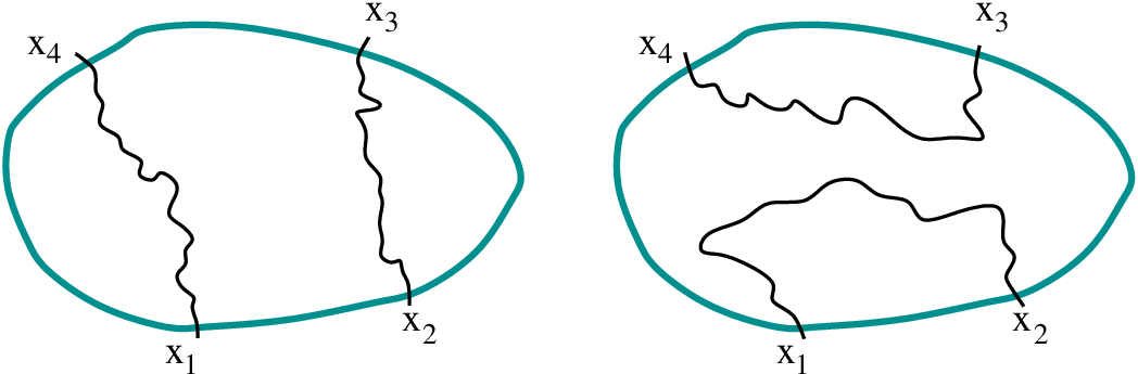
By conformal invariance we may normalize the points so that , , and with . We have two distinct topological configurations and we thus have to identify the two corresponding pure partition functions. This is will be done by specifying the way the partition functions behave when points are fused together. By construction these partition functions may be written as correlation functions
so that their behavior when points are fused are governed by CFT fusion rules. As a consequence, behave either as or as as .
We select the pure partition functions and by demanding that:
| (9) | |||||
and so that
will turn out to be the pure partition function for configurations in which the curves join the pairs and while will turn out to correspond to the configurations and . The rationale behind these conditions consists in imposing that the pure partition function possesses the leading singularity, with exponent , when is approaching the point allowed by the configuration but has subleading singularity, with exponent , when is approaching the point forbidden by the configuration.
This set of conditions uniquely determines the functions and . These follows from CFT rules but may also be checked by explicitly solving the differential equation that these functions satisfy. Writing yields,
so that is an hypergeometric function and
with the constant chosen to normalize as above. Using this explicit formula one may verify that is effectively a positive number for any so it has all expected properties to be a pure partition function.
For , and for , .
8.2.2 Arch probabilities
Let us now compute the probabilities for having one of the two topologically distinct configurations: either with curves joining either and or with curves joining and as we just discussed. We shall proceed blindly, but the reader should beware that there are subtleties involved. What is computed is the probability for certain ’s to hit each other. What happens at the level of hulls and how the process should be properly continued is not investigated, but is expected to yield the announced probability for arch configuration.
We consider a generic partition function which is the sum of the pure partition functions and :
with and positive. To specify the 3SLE (or 4SLE) process we need the partition function which is recover from by conformal transformation :
with the harmonic ratio of the four points , , and :
Let and be defined by
By construction the processes and , with the harmonic ratio of the four moving points, are local martingales. Since both and are positive, are are bounded local martingales and thus are martingales.
Let be the stopping time given by the first instant at which a pair of points coincide. Then, in configuration we have while in configuration . Since, for , is such that but , we obtain that evaluated at the stopping time is the characteristic function for events with the topological configuration , ie:
Since and are martingales, we get the probability of occurrence of configurations of topological type :
| (10) |
and similarly for the probabilities of having configuration . As expected they are ratios of partition functions.
8.3 Applications to percolation and Ising model
We are now ready to give an application of triple (or quadruple) SLE to percolation and Ising model. Exploration processes in critical percolation are described by SLEs with , as proved in [19]. Interfaces of spin clusters in critical Ising model is believed to correspond to while interfaces of Fortuin-Kasteleyn clusters – which occur in a high temperature expansion of the Ising partition function – are expected to correspond to the dual value .
What we have in mind are these statistical models, defined on the upper half plane, with boundary condition changing operators at the four points and . They change the boundary condition from open to closed (or vice versa) in percolation and from plus to minus (or vice versa) for Ising model .
To apply previous results on 4SLE processes to these situations, we have to specify the partition functions , or equivalently, we have to specify the value of and . This is done by noticing that these models are left-right symmetric so that for there is equal probability to find configuration or . Since , we have , so that the total partition function is and the probability of occurrence of configuration for any is now:
– Percolation corresponds to . The boundary changing operator has dimension . The pure partition function has a simple integral representation:
By construction also possesses a simple integral representation but, most importantly, it is such that the total partition function is constant, , as expected for percolation. As a consequence we find:
This is nothing but Cardy percolation crossing formula.
– Ising spin clusters correspond to . The boundary changing operator has dimension and may thus be identified with a fermion on the boundary. However the pure partition functions do not correspond to the free fermion conformal block. By solving the differential equation with the appropriate boundary condition we get:
The total partition function is proportional to , which is the free fermion result.
Hence, the Ising configuration probabilities are :
This is nothing but a new – and previously unknown – Ising crossing formula.
– FK Ising clusters correspond to . The operator has then dimension . The pure partition function are given by:
and the crossing probabilities by:
The other critical random cluster (or Potts) models with have , and it is straightforward to obtain explicit crossing formulas involving only hypergeometric functions.
8.4 nSLEs and beyond
We now comment on how to compute multiple arch probabilities for
general nSLEs. This section only aims at giving some hints on how to
generalize previous computations. So it shall be sketchy. It is clear
that the key point is to identify the pure partition functions – once
this is done the rest is routine. As exemplified above by
eq.(9) this is linked to CFT fusions. The rules there were
that, for a given arch system, fusing two points linked by an arch
produces the dominant singularity which means that the two boundary
operators are fused on the identity operator, whereas fusing two
points not linked by an arch produces the subleading singularity which
means the fusion of the two boundary fields on the identity should
vanish. In general there could be a whole hierarchy of arches with
arches in the interior of others, i.e. with a family of self-surrounding
arches, the next encircling the previous.
So we are lead to propose the following rules.
For a given arch configuration:
— The most interior pair of adjacent pair of points, say
in a family of self-surrounding arches fused into the
identity operator, so that the pure partition function evaluated at
should be proportional to
times the pure partition
function associated to the arch system with the interior arch
removed. Symbolically :
for and linked by an arch.
— The fusion on the identity of any pair of adjacent points
not linked by an arch should vanish, so that the fusion of this
pair of points produces the subleading singularity. Symbolically :
for and for not linked by an arch.
We do not have a complete proof that these rules fully determine the pure partition functions but we checked it on a few cases, see figure 7.

Here are a few samples. We shall give the relation between the pure partition and the CFT conformal blocks indexed by the corresponding Bratelli diagram. For , we may have the following arch systems or . (A given geometrical configuration may correspond to different arch systems depending at which location we open the closed boundary. But they are all equivalent to these two up to an order preserving relabeling of the points. For instance is equivalent to .) Applying the previous rules we get:
where the indices , refer to the corresponding points in the Bratelli diagram, i.e. to the weights of the intermediate Virasoro modules. The coefficient is fully determined, in terms of CFT fusion coefficients, by demanding that the fusion of and on the identity vanishes.
One may go on and solve for the pure partition functions in few other cases. A particularly simple example with is given by :
As can be seen on these examples, there is no simple relation between arch systems and Bratelli diagrams and the change of basis for one to the other is quite involved. The only simple rule we find is that the pure partition function for a unique family of self-surrounding arches is a pure conformal block corresponding to a unique Bratelli diagram.
References
- [1] O. Schramm, Israel J. Math., 118, 221-288, (2000);
- [2] S. Rohde, O. Schramm “Basic Properties of SLE” Ann. Math., to appear, 2001 [arXiv:math.PR/0106036].
- [3]
W. Werner
“Random planar curves and Schramm-Loewner evolutions”
In Lectures on probability theory and statistics,
vol. 1840 of Lecture Notes in Math., p. 107-195.
[arXiv:math.PR/0303354]
Springer, Berlin, 2004 . - [4] G. Lawler, O. Schramm, W. Werner “Conformal restriction. The chordal case” to appear in JAMS [arXiv:math.PR/0209343].
- [5]
G. Lawler, O. Schramm and W. Werner,
(I): Acta Mathematica 187 (2001) 237-273; arXiv:math.PR/9911084
G. Lawler, O. Schramm and W. Werner, (II): Acta Mathematica 187 (2001) 275-308; arXiv:math.PR/0003156
G. Lawler, O. Schramm and W. Werner, (III): Ann. Henri Poincaré 38 (2002) 109-123. arXiv:math.PR/0005294. - [6] J. Dubedat “SLE() martingales and duality” to appear in Ann. Probab., 2003 [arXiv:math.PR/].
- [7] M. Bauer and D. Bernard, “Conformal field theories of stochastic Loewner evolutions” Commun. Math. Phys. 239 (2003) 493 [arXiv:hep-th/0210015].
- [8] M. Bauer and D. Bernard, “SLE(kappa) growth processes and conformal field theories” Phys. Lett. B 543 (2002) 135 [arXiv:math-ph/0206028].
- [9] R. Friedrich and W. Werner, “Conformal restriction, highest weight representations and SLE”, [arXiv:math-ph/0301018].
- [10] M. Bauer and D. Bernard, “SLE martingales and the Virasoro algebra,” Phys. Lett. B 557 (2003) 309 [arXiv:hep-th/0301064].
- [11] M. Bauer and D. Bernard, “Conformal transformations and the SLE partition function martingale” Annales Henri Poincare 5 (2004) 289 [arXiv:math-ph/0305061].
- [12] M. Bauer and D. Bernard, “CFTs of SLEs: The radial case” Phys. Lett. B 583 (2004) 324 [arXiv:math-ph/0310032].
- [13] M. Bauer and D. Bernard, “SLE, CFT and zig-zag probabilities” [arXiv:math-ph/0401019].
- [14] M. Bauer, D. Bernard and J. Houdayer, “Dipolar SLEs” [arXiv:math-ph/0411038].
- [15] J. Cardy, “Stochastic Loewner evolution and Dysons circular ensembles”, J. Phys. A: Math. Gen. 36 (2003) L379-L386 [arXiv:math-ph/0301039].
- [16] J. Dubedat “Some remarks on commutation relations for SLE” (2004) [arXiv:math.PR/0411299].
- [17] A. Belavin, A. Polyakov, A. Zamolodchikov: “Infinite conformal symmetry in two-dimensional quantum field theory”, Nucl. Phys. B241, 333-380, (1984).
- [18]
P. Di Francesco, P. Mathieu, D. Sénéchal:
“Conformal Field Theory”
Springer-Verlag New York, Inc., 1997 - [19] S. Smirnov: “Critical percolation in the plane” C. R. Acad. Sci. Paris Sér. I Math., 333 (2001), no. 3, 239-244.