Homotopy of posets, net-cohomology and superselection sectors in globally hyperbolic spacetimes

Giuseppe Ruzzi Affiliation: Dipartimento di Matematica, Università di Roma “Tor Vergata” Affiliation: Via della Ricerca Scientifica, 00133, Roma, Italy Email: ruzzi@mat.uniroma2.it

Abstract

We study sharply localized sectors, known as sectors of DHR-type, of a net of local observables, in arbitrary globally hyperbolic spacetimes with dimension $\geq 3$ . We show that these sectors define, has it happens in Minkowski space, a $\mathrm{C}^{*}-$ category in which the charge structure manifests itself by the existence of a tensor product, a permutation symmetry and a conjugation. The mathematical framework is that of the net-cohomology of posets according to J.E. Roberts. The net of local observables is indexed by a poset formed by a basis for the topology of the spacetime ordered under inclusion. The category of sectors, is equivalent to the category of 1-cocycles of the poset with values in the net. We succeed to analyze the structure of this category because we show how topological properties of the spacetime are encoded in the poset used as index set: the first homotopy group of a poset is introduced and it is shown that the fundamental group of the poset and the one of the underlying spacetime are isomorphic; any 1-cocycle defines a unitary representation of these fundamental groups. Another important result is the invariance of the net-cohomology under a suitable change of index set of the net.

1 Introduction

The present paper is concerned with the study of charged superselection sectors in globally hyperbolic spacetimes in the framework of the algebraic approach to quantum field theory [18, 19]. The basic object of this approach is the abstract net of local observables $\mathscr{R}_{\mathcal{K}}$ , namely the correspondence

\mathcal{K}\ni\mathcal{O}\rightarrow\mathcal{R}(\mathcal{O}),

which associates to any element $\mathcal{O}$ of a family $\mathcal{K}$ of relatively compact open regions of the spacetime $\mathcal{M}$ , considered as a fixed background manifold, the $\mathrm{C}^{*}-$ algebra $\mathcal{R}(\mathcal{O})$ generated by all the observables which are measurable within $\mathcal{O}$ . Sectors are unitary equivalence classes of irreducible representations of this net, the labels distinguishing different classes are the quantum numbers. The study of physically meaningful sectors of the net of local observables, and how to select them, is the realm of the theory of superselection sectors.
One of the main results of superselection sectors theory has been the demonstration that in Minkowski space $\mathbb{M}^{4}$ , among the representations of the net of local observables it is possible to select a family of sectors whose quantum numbers manifest the same properties as the charges carried by elementary particles: a composition law, the alternative of Bose and Fermi statistics and the charge conjugation symmetry. The first example of sectors manifesting these properties has been provided in [11, 12], known as DHR-analysis, where the authors investigated sharply localized sectors. Namely, a representation $\pi$ of $\mathscr{R}_{\mathcal{K}}$ is a sector of DHR-type whenever its restriction to the spacelike complement $\mathcal{O}^{\perp}$ of any element $\mathcal{O}$ of $\mathcal{K}$ is unitary equivalent to the vacuum representation $\pi_{o}$ of the net, in symbols

\pi|_{\mathcal{R}(\mathcal{O}^{\perp})}\cong\pi_{o}|_{\mathcal{R}(\mathcal{O}^{\perp})},\qquad\mathcal{O}\in\mathcal{K}.

(1)

Although no known charge present in nature is sharply localized, the importance of the DHR-analysis resides in the following reasons. First, it suggests the idea that physically charged sectors might be localized in a more generalized sense with respect to (1). Secondly, the introduction of powerful techniques based only on the causal structure of the Minkowski space that can be used to investigate other types of localized sectors. A relevant example are the BF-sectors [4] which describe charges in purely massive theories. BF-sectors are localized in spacelike cones, which are a family of noncompact regions of $\mathbb{M}^{4}$ . In curved spacetimes the nontrivial topology can induce superselection sectors, see [2] and references quoted therein. However, up until now, the localization properties of these sectors are not known, hence it is still not possible to investigate their charge structure.
In the present paper we deal with the study of sectors of DHR-type in arbitrary globally hyperbolic spacetimes. Because of the sharp localization, sectors of DHR-type should be insensitive to the nontrivial topology of the spacetime, and their quantum numbers should exhibit the same features as in Minkowski space. However, the first investigations [17, 28] have provided only partial results in this direction, and, in particular, they have pointed out that for particular classes of spacetimes the topology might affect the properties of sectors of DHR-type. The aim of the present paper is to show how this type of sectors and the topology of spacetime are related and that they manifest the properties described above also in an arbitrary globally hyperbolic spacetime. We want to stress that the results of this paper are confined to spacetimes whose dimension is $\geq 3$ .
Before entering the theory of DHR-sectors in globally hyperbolic spacetimes, a key fact has still to be mentioned. The DHR-analysis can be equivalently read in terms of net-cohomology of posets, a cohomological approach initiated and developed by J.E. Roberts [26], (see also [27, 28] and references therein). Such an approach makes clear that the spacetime information which is relevant for the analysis of the DHR-sectors is the topological and the causal structure of Minkowski space (the Poincaré symmetry enters the theory only in the definition of the vacuum representation). In particular, the essential point is how these two properties are encoded in the structure of the index $\mathcal{K}$ as a partially ordered set (poset) with respect to inclusion order relation $\subseteq$ . Representations satisfying (1) are, up to equivalence, in 1-1 correspondence with 1-cocycles $z$ of the poset $\mathcal{K}$ with values in the vacuum representation of the net $\mathscr{A}_{\mathcal{K}}:\mathcal{O}\rightarrow\mathcal{A}(\mathcal{O})$ . Here $\mathcal{A}(\mathcal{O})$ is the von Neumann algebra obtained by taking the bicommutant $\pi_{o}(\mathcal{R}(\mathcal{O}))^{\prime\prime}$ of $\pi_{o}(\mathcal{R}(\mathcal{O}))$ . These 1-cocycles, which are nothing but the charge transporters of DHR-analysis, define a tensor $\mathrm{C}^{*}-$ category $\mathcal{Z}^{1}_{t}(\mathscr{A}_{\mathcal{K}})$ with a permutation symmetry and conjugation.
The first investigation of sectors of DHR-type in a globally hyperbolic spacetime $\mathcal{M}$ has been done in [17]. First, the authors consider the net of local observables $\mathscr{R}_{\mathcal{K}_{\diamond}}$ indexed by the set $\mathcal{K}_{\diamond}$ of regular diamonds of $\mathcal{M}$ : a family of relatively compact open sets codifying the topological and the causal properties of $\mathcal{M}$ . Secondly, they take a reference representation $\pi_{o}$ of $\mathscr{R}_{\mathcal{K}_{\diamond}}$ on a Hilbert space $\mathcal{H}_{o}$ such that the net $\mathscr{A}_{\mathcal{K}_{\diamond}}:\mathcal{K}_{\diamond}\ni\mathcal{O}\rightarrow\mathcal{A}(\mathcal{O})\equiv\pi_{o}(\mathcal{R}(\mathcal{O}))^{\prime\prime}$ satisfies Haag duality and the Borchers property (see Section 4). The reference representation $\pi_{o}$ plays for the theory the same role that the vacuum representation plays in the case of Minkowski space. Examples of physically meaningful nets of local algebras indexed by regular diamonds have been given in [33]. Finally, the DHR-sectors are singled out from the representations of the net $\mathscr{R}_{\mathcal{K}_{\diamond}}$ by generalizing, in a suitable way, the criterion (1). As in Minkowski space, the physical content of DHR-sectors is contained in the $\mathrm{C}^{*}-$ category $\mathcal{Z}^{1}_{t}(\mathscr{A}_{\mathcal{K}_{\diamond}})$ of 1-cocycles of $\mathcal{K}_{\diamond}$ with values in $\mathscr{A}_{\mathcal{K}_{\diamond}}$ , and when $\mathcal{K}_{\diamond}$ is directed under inclusion, there exist a tensor product, a symmetry and conjugated 1-cocycles. The analogy with the theory in the Minkowski space breaks down when the $\mathcal{K}_{\diamond}$ is not directed. In this situation only the introduction of a tensor product on $\mathcal{Z}^{1}_{t}(\mathscr{A}_{\mathcal{K}_{\diamond}})$ and the existence of a symmetry have been achieved in [17], although the definition of the tensor product is not completely discussed (see below).
There are two well known topological conditions on the spacetime, implying that not only regular diamonds but any reasonable set of indices for a net of local algebras is not directed: this happens when the spacetime is either nonsimply connected or has compact Cauchy surfaces (Corollary 2.19 and Lemma 3.2). There arises, therefore, the necessity to understand the connection between net-cohomology and topology of the underlying spacetime. Progress in this direction has been achieved in [28]. The homotopy of paths, the net-cohomology under a change of the index set are issues developed in that work that will turn out to be fundamental for our aim. Moreover, it has been shown that the statistics of sectors can be classified provided that the net satisfies punctured Haag duality (see Section 4). However, no result concerning the conjugation has been achieved.
To see what is the main drawback caused by the non directness of the poset $\mathcal{K}_{\diamond}$ , we have to describe more in detail $\mathcal{Z}^{1}_{t}(\mathscr{A}_{\mathcal{K}_{\diamond}})$ . The elements $z$ of $\mathcal{Z}^{1}_{t}(\mathscr{A}_{\mathcal{K}_{\diamond}})$ are 1-cocycles trivial in $\mathfrak{B}(\mathcal{H}_{o})$ or, equivalently, path-independent on $\mathcal{K}_{\diamond}$ . The latter means that the evaluation of $z$ on a path of $\mathcal{K}_{\diamond}$ depends only on the endpoints of the path. When $\mathcal{K}_{\diamond}$ is directed any 1-cocycle is trivial in $\mathfrak{B}(\mathcal{H}_{o})$ , but this might not be hold when $\mathcal{K}_{\diamond}$ is not directed. The consequences can be easily showed: let $\widehat{\otimes}$ be the tensor product introduced in [17]: for any $z,z_{1}\in\mathcal{Z}^{1}_{t}(\mathscr{A}_{\mathcal{K}_{\diamond}})$ , it turns out that $z\widehat{\otimes}z_{1}$ is a 1-cocycle of $\mathcal{K}_{\diamond}$ with values in $\mathscr{A}_{\mathcal{K}_{\diamond}}$ , but it is not clear whether it is trivial in $\mathfrak{B}(\mathcal{H}_{o})$ (we will see in Remark 4.18 that this 1-cocycle is trivial in $\mathfrak{B}(\mathcal{H}_{o})$ ). Now, we know that the nonsimply connectedness and the compactness of the Cauchy surfaces are topological obstructions to the directness of the index sets. The first aim of this paper is to understand whether these conditions are also obstructions to the triviality in $\mathfrak{B}(\mathcal{H}_{o})$ of 1-cocycles. This problem is analyzed in great generality in Section 2. We introduce the notions of the first homotopy group and fundamental group for an abstract poset $\mathcal{P}$ (Definition 2.4) and prove that any 1-cocycle $z$ of $\mathcal{P}$ , with values in a net of local algebras $\mathscr{A}_{\mathcal{P}}$ indexed by $\mathcal{P}$ , defines a unitary representation of the fundamental group of $\mathcal{P}$ (Theorem 2.8). In the case that $\mathcal{P}$ is a basis for a topological space ordered under inclusion, and whose elements are arcwise and simply connected sets, then the fundamental group of $\mathcal{P}$ is isomorphic to the fundamental group of the underlying topological space (Theorem 2.18). This states that the only possible topological obstruction to the triviality in $\mathfrak{B}(\mathcal{H}_{o})$ of 1-cocycles is the nonsimply connectedness (Corollary 2.21).
Before studying superselection sectors in a globally hyperbolic spacetime $\mathcal{M}$ , we have to point out another problem arising in [17, 28]. Regular diamonds do not need to have arcwise connected causal complements. This, on the one hand creates some technical problems; on the other hand it is not clear whether it is justified to assume Haag duality on $\mathscr{A}_{\mathcal{K}_{\diamond}}$ : the only known result showing that a net of local observables, in the presence of a nontrivial superselection structure, inherits Haag duality from fields makes use of the arcwise connectedness of causal complements of the elements of the index set [17, Theorem 3.15]. We start to deal with this problem by showing that net-cohomology is invariant under a change of the index set (Theorem 2.23), provided the new index set is a refinement of $\mathcal{K}_{\diamond}$ (see Definition 2.9 and Lemma 2.22a). In Section 3.2 we introduce the set $\mathcal{K}$ of diamonds of $\mathcal{M}$ . $\mathcal{K}$ is a refinement of $\mathcal{K}_{\diamond}$ and any element of $\mathcal{K}$ has an arcwise connected causal complement. Therefore adopting $\mathcal{K}$ as index set the cited problems are overcome.
In Section 4, we consider an irreducible net $\mathscr{A}_{\mathcal{K}}$ satisfying the Borchers property and punctured Haag duality. The key for studying superselection sectors of the net $\mathscr{A}_{\mathcal{K}}$ , namely the $\mathrm{C}^{*}-$ category $\mathcal{Z}^{1}_{t}(\mathscr{A}_{\mathcal{K}})$ , is provided by the following fact. We introduce the causal puncture $\mathcal{K}_{x}$ of $\mathcal{K}$ induced by a point $x$ of $\mathcal{M}$ (17) and consider the categories $\mathcal{Z}^{1}_{t}(\mathscr{A}_{\mathcal{K}_{x}})$ of 1-cocycles of $\mathcal{K}_{x}$ , trivial in $\mathfrak{B}(\mathcal{H}_{o})$ , with values in the net $\mathscr{A}_{\mathcal{K}_{x}}$ . We show that a family $z_{x}\in\mathcal{Z}^{1}_{t}(\mathscr{A}_{\mathcal{K}_{x}})$ for any $x\in\mathcal{M}$ admits an extension to a 1-cocycle $z\in\mathcal{Z}^{1}_{t}(\mathscr{A}_{\mathcal{K}})$ if, and only if, a suitable gluing condition is verified (Proposition 4.2). A similar result holds for arrows (Proposition 4.3), and can be easily generalized to functors. These results suggest that one could proceed as follows: first, prove that the categories $\mathcal{Z}^{1}_{t}(\mathscr{A}_{\mathcal{K}_{x}})$ have the right structure to describe the superselection theory (local theory, Section 4.2); secondly, check that the constructions we have made on $\mathcal{Z}^{1}_{t}(\mathscr{A}_{\mathcal{K}_{x}})$ satisfy the mentioned gluing condition, and consequently can be extended to $\mathcal{Z}^{1}_{t}(\mathscr{A}_{\mathcal{K}})$ (global theory, Section 4.3). This argument works. We will prove that $\mathcal{Z}^{1}_{t}(\mathscr{A}_{\mathcal{K}})$ has a tensor product, a symmetry and that any object has left inverses. The full subcategory $\mathcal{Z}^{1}_{t}(\mathscr{A}_{\mathcal{K}})_{\mathrm{f}}$ of $\mathcal{Z}^{1}_{t}(\mathscr{A}_{\mathcal{K}})$ whose objects have finite statistics has conjugates (Theorem 4.15).
In Appendix A we give some basics definitions and results on tensor $\mathrm{C}^{*}-$ categories.

2 Homotopy and net-cohomology of posets

After some preliminaries, the main topics are discussed in full generality in the first three sections: the first homotopy group of a poset; the connection between homotopy and net-cohomology; the behaviour of net-cohomology under a change of the index set. The remaining two sections are devoted to study the case that the poset is a basis for the topology of a topological space. We stress that the results obtained in the first three sections in terms of abstract posets can be applied, not only to sharply localized charges which are the subject of the present investigation, but also to charges like those studied in [4, 2].

2.1 Preliminaries: the simplicial set and net-cohomology

In the present section we recall the definition of simplicial set of a poset and the notion of net-cohomology of a poset, thereby establishing our notations. References for this section are [27, 17, 28].
The simplicial set - A poset $(\mathcal{P},\leq)$ is a partially ordered set. This means that $\leq$ is a binary relation on a nonempty set $\mathcal{P}$ , satisfying

\begin{array}[]{lcll}\mbox{for any }\mathcal{O}\in\mathcal{P}&\Rightarrow&\mathcal{O}\leq\mathcal{O}&reflexive\\ \mathcal{O}_{1}\leq\mathcal{O}_{2}\mbox{ and }\mathcal{O}_{2}\leq\mathcal{O}_{1}&\Rightarrow&\mathcal{O}_{1}=\mathcal{O}_{2}&antisymmetric\\ \mathcal{O}_{1}\leq\mathcal{O}_{2}\mbox{ and }\mathcal{O}_{2}\leq\mathcal{O}_{3}&\Rightarrow&\mathcal{O}_{1}\leq\mathcal{O}_{3}&transitive\end{array}

A poset is said to be directed if for any pair $\mathcal{O}_{1},\mathcal{O}_{2}\in\mathcal{P}$ there exists $\mathcal{O}_{3}\in\mathcal{P}$ such that $\mathcal{O}_{1},\mathcal{O}_{2}\leq\mathcal{O}_{3}$ . For our aim, important examples of posets are provided by the standard simplices. A standard $n-simplex$ is defined as

\Delta_{n}\equiv\big\{(\lambda_{0},\ldots,\lambda_{n})\in\mathbb{R}^{n+1}\ |\ \lambda_{0}+\cdots+\lambda_{n}=1,\ \ \lambda_{i}\in[0,1]\big\}.

It is clear that $\Delta_{0}$ is a point, $\Delta_{1}$ is a closed interval etc… The inclusion maps $d^{n}_{i}$ between standard simplices are maps $d^{n}_{i}:\Delta_{n-1}\longrightarrow\Delta_{n}$ defined as

d^{n}_{i}(\lambda_{0},\ldots,\lambda_{n-1})=(\lambda_{0},\lambda_{1},\ldots,\lambda_{i-1},0,\lambda_{i},\ldots\lambda_{n-1}),

for $n\geq 1$ and $0\leq i\leq n$ . Now, note that a standard n-simplex $\Delta_{n}$ can be regarded as a partially ordered set with respect to the inclusion of its subsimplices. A singular n-simplex of a poset $\mathcal{P}$ is an order preserving map $f:\Delta_{n}\longrightarrow\mathcal{P}$ . We denote by $\Sigma_{n}(\mathcal{P})$ the collection of singular n-simplices of $\mathcal{P}$ and by $\Sigma_{*}(\mathcal{P})$ the collection of all singular simplices of $\mathcal{P}$ . $\Sigma_{*}(\mathcal{P})$ is the simplicial set of $\mathcal{P}$ . The inclusion maps $d^{n}_{i}$ between standard simplices are extended to maps $\partial^{n}_{i}:\Sigma_{n}(\mathcal{P})\longrightarrow\Sigma_{n-1}(\mathcal{P})$ , called boundaries, between singular simplices by setting $\partial^{n}_{i}f\equiv f\circ d^{n}_{i}$ . One can easily check, by the definition of $d^{n}_{i}$ , that the following relations

\partial^{n-1}_{i}\circ\partial^{n}_{j}=\partial^{n-1}_{j}\circ\partial^{n}_{i+1},\qquad i\geq j,

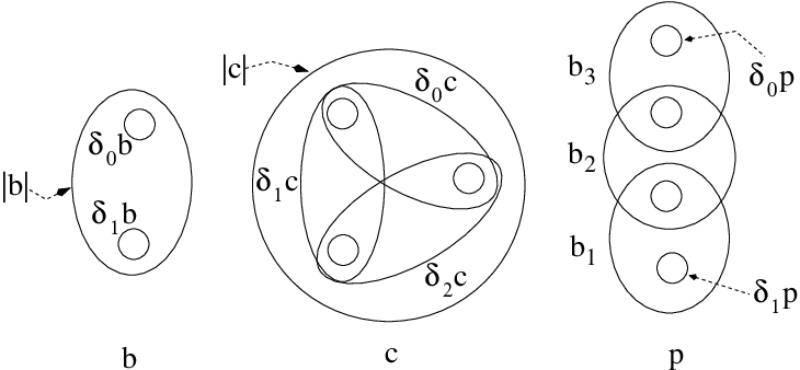
hold. From now on, we will omit the superscripts from the symbol $\partial^{n}_{i}$ , and will denote: the composition $\partial_{i}\circ\partial_{j}$ by the symbol $\partial_{ij}$ ; 0-simplices by the letter $a$ ; 1-simplices by $b$ and 2-simplices by $c$ . Notice that a 0-simplex $a$ is nothing but an element of $\mathcal{P}$ ; a 1-simplex $b$ is formed by two 0-simplices $\partial_{0}b$ , $\partial_{1}b$ and an element $|b|$ of $\mathcal{P}$ , called the support of $b$ , such that $\partial_{0}b$ , $\partial_{1}b\leq|b|$ . Given $a_{0},a_{1}\in\Sigma_{0}(\mathcal{P})$ , a path from $a_{0}$ to $a_{1}$ is a finite ordered sequence $p=\{b_{n},\ldots,b_{1}\}$ of 1-simplices satisfying the relations

\partial_{1}b_{1}=a_{0},\ \ \ \partial_{0}b_{i}=\partial_{1}b_{i+1}\ \mbox{ with }\ i\in\{1,\ldots,n-1\},\ \ \ \partial_{0}b_{n}=a_{1}.

The startingpoint of $p$ , written $\partial_{1}p$ , is the 0-simplex $a_{0}$ , while the endpoint of $p$ , written $\partial_{0}p$ , is the 0-simplex $a_{1}$ . We will denote by $\mathrm{P}(a_{0},a_{1})$ the set of paths from $a_{0}$ to $a_{1}$ , and by $\mathrm{P}(a_{0})$ the set of closed paths with endpoint $a_{0}$ . $\mathcal{P}$ is said to be pathwise connected whenever for any pair $a_{0},a_{1}$ of 0-simplices there exists a path $p\in\mathrm{P}(a_{0},a_{1})$ . The support of the path is the collection $|p|\equiv\{|b_{i}|\ |\ i=1,\ldots,n\}$ , and we will write $|p|\subseteq P$ if $P$ is a subset of $\mathcal{P}$ with $|b_{i}|\in P$ for any $i$ . Furthermore, with an abuse of notation, we will write $|p|\subseteq\mathcal{O}$ if $\mathcal{O}\in\mathcal{P}$ with $|b_{i}|\leq\mathcal{O}$ for any $i$ .

Refer to caption — Figure 1: $b$ is a 1-simplex, $c$ is a 2-simplex, $p=\{b_{3},b_{2},b_{1}\}$ is a path. The symbol $\delta$ stands for $\partial$ .

Causal disjointness and net of local algebras - Given a poset $\mathcal{P}$ , a causal disjointness relation on $\mathcal{P}$ is a symmetric binary relation $\perp$ on $\mathcal{P}$ satisfying the following properties:

\begin{array}[]{ll}\mbox{(i)}&\mathcal{O}_{1}\in\mathcal{P}\ \Rightarrow\ \exists\mathcal{O}_{2}\in\mathcal{P}\mbox{ such that }\ \mathcal{O}_{1}\perp\mathcal{O}_{2};\\ \mbox{(ii)}&\mathcal{O}_{1}\leq\mathcal{O}_{2}\mbox{ and }\mathcal{O}_{2}\perp\mathcal{O}_{3}\ \Rightarrow\ \mathcal{O}_{1}\perp\mathcal{O}_{3};\\ \end{array}

(2)

Given a subset $P\subseteq\mathcal{P}$ , the causal complement of $P$ is the subset $P^{\perp}$ of $\mathcal{P}$ defined as

P^{\perp}\equiv\{\mathcal{O}\in\mathcal{P}\ |\ \mathcal{O}\perp\mathcal{O}_{1},\ \forall\mathcal{O}_{1}\in P\}.

Note that if $P_{1}\subseteq P$ , then $P^{\perp}\subseteq P^{\perp}_{1}$ . Now, assume that $\mathcal{P}$ is a pathwise connected poset equipped with a causal disjointness relation $\perp$ . A net of local algebras indexed by $\mathcal{P}$ is a correspondence

\mathscr{A}_{\mathcal{P}}:\mathcal{P}\ni\mathcal{O}\longrightarrow\mathcal{A}(\mathcal{O})\subseteq\mathfrak{B}(\mathcal{H}_{o}),

associating to any $\mathcal{O}$ a von Neumann algebras $\mathcal{A}(\mathcal{O})$ defined on a fixed Hilbert space $\mathcal{H}_{o}$ , and satisfying

\begin{array}[]{lcll}\mathcal{O}_{1}\leq\mathcal{O}_{2}&\Rightarrow&\mathcal{A}(\mathcal{O}_{1})\subseteq\mathcal{A}(\mathcal{O}_{2}),&\qquad isotony,\\ \mathcal{O}_{1}\perp\mathcal{O}_{2}&\Rightarrow&\mathcal{A}(\mathcal{O}_{1})\subseteq\mathcal{A}(\mathcal{O}_{2})^{\prime},&\qquad causality,\end{array}

where the prime over the algebra stands for the commutant of the algebra. The algebra $\mathcal{A}(\mathcal{O}^{\perp})$ associated with the causal complement $\mathcal{O}^{\perp}$ of $\mathcal{O}\in\mathcal{P}$ , is the $\mathrm{C}^{*}-$ algebra generated by the algebras $\mathcal{A}(\mathcal{O}_{1})$ for any $\mathcal{O}_{1}\in\mathcal{P}$ with $\mathcal{O}_{1}\perp\mathcal{O}$ . The net $\mathscr{A}_{\mathcal{P}}$ is said to be irreducible whenever, given $T\in\mathfrak{B}(\mathcal{H}_{o})$ such that $T\in\mathcal{A}(\mathcal{O})^{\prime}$ for any $\mathcal{O}\in\mathcal{P}$ , then $T=c\cdot\mathbbm{1}$ .
The category of 1-cocycles - We refer the reader to the Appendix for the definition of $\mathrm{C}^{*}-$ category. Let $\mathcal{P}$ be a poset with a causal disjointness relation $\perp$ , and let $\mathscr{A}_{\mathcal{P}}$ be an irreducible net of local algebras. A 1-cocycle $z$ of $\mathcal{P}$ with values in $\mathscr{A}_{\mathcal{P}}$ is a field $z:\Sigma_{1}(\mathcal{P})\ni b\longrightarrow z(b)\in\mathfrak{B}(\mathcal{H}_{o})$ of unitary operators satisfying the 1-cocycle identity:

z(\partial_{0}c)\cdot z(\partial_{2}c)=z(\partial_{1}c),\qquad c\in\Sigma_{2}(\mathcal{P}),

and the locality condition: $z(b)\in\mathcal{A}(|b|)$ for any 1-simplex $b$ . An intertwiner $t\in(z,z_{1})$ between a pair of 1-cocycles $z,z_{1}$ is a field $t:\Sigma_{0}(\mathcal{P})\ni a\longrightarrow t_{a}\in\mathfrak{B}(\mathcal{H}_{o})$ satisfying the relation

t_{\partial_{0}b}\cdot z(b)=z_{1}(b)\cdot t_{\partial_{1}b},\qquad b\in\Sigma_{1}(\mathcal{P}),

and the locality condition: $t_{a}\in\mathcal{A}(a)$ for any 0-simplex $a$ . The category of 1-cocycles $\mathcal{Z}^{1}(\mathscr{A}_{\mathcal{P}})$ is the category whose objects are 1-cocycles and whose arrows are the corresponding set of intertwiners. The composition between $s\in(z,z_{1})$ and $t\in(z_{1},z_{2})$ is the arrow $t\cdot s\in(z,z_{2})$ defined as

(t\cdot s)_{a}\equiv t_{a}\cdot s_{a},\qquad a\in\Sigma_{0}(\mathcal{P}).

Note that the arrow $1_{z}$ of $(z,z)$ defined as $(1_{z})_{a}=\mathbbm{1}$ , for any $a\in\Sigma_{0}(\mathcal{P})$ , is the identity of $(z,z)$ . Now, the set $(z,z_{1})$ has a structure of complex vector space defined as

(\alpha\cdot t+\beta\cdot s)_{a}\equiv\alpha\cdot t_{a}+\beta\cdot s_{a},\qquad a\in\Sigma_{0}(\mathcal{P}),

for any $\alpha,\beta\in\mathbb{C}$ and $t,s\in(z,z_{1})$ . With these operations and the composition “ $\cdot$ ”, the set $(z,z)$ is an algebra with identity $1_{z}$ . The category $\mathcal{Z}^{1}(\mathscr{A}_{\mathcal{P}})$ has an adjoint $*$ , defined on as the identity, $z^{*}=z$ , on the objects, while the adjoint $t^{*}\in(z_{1},z)$ of on arrows $t\in(z,z_{1})$ is defined as

(t^{*})_{a}\equiv(t_{a})^{*},\qquad a\in\Sigma_{0}(\mathcal{P}),

where $(t_{a})^{*}$ stands for the adjoint in $\mathfrak{B}(\mathcal{H}_{o})$ of the operator $t_{a}$ . Now, let $\|{\ }\|$ be the norm of $\mathfrak{B}(\mathcal{H}_{o})$ . Given $t\in(z,z_{1})$ , we have that $\|{t_{a}}\|=\|{t_{a_{1}}}\|$ for any pair $a,a_{1}$ of 0-simplices because $\mathcal{P}$ is pathwise connected. Therefore, by defining

\|{t}\|\equiv\|{t_{a}}\|\qquad a\in\Sigma_{0}(\mathcal{P})

it turns out $(z,z_{1})$ is a complex Banach space for any $z,z_{1}\in\mathcal{Z}^{1}(\mathscr{A}_{\mathcal{P}})$ , while $(z,z)$ is a $\mathrm{C}^{*}-$ algebra for any $z\in\mathcal{Z}^{1}(\mathscr{A}_{\mathcal{P}})$ . This entails that $\mathcal{Z}^{1}(\mathscr{A}_{\mathcal{P}})$ is a $\mathrm{C}^{*}-$ category. Two 1-cocycles $z,z_{1}$ are equivalent (or cohomologous) if there exists a unitary arrow $t\in(z,z_{1})$ . A 1-cocycle $z$ is trivial if it is equivalent to the identity cocycle $\iota$ defined as $\iota(b)=\mathbbm{1}$ for any 1-simplex $b$ . Note that, since $\mathscr{A}_{\mathcal{P}}$ is irreducible, $\iota$ is irreducible: $(\iota,\iota)=\mathbb{C}\mathbbm{1}$ .
Equivalence in $\boldsymbol{\mathfrak{B}(\mathcal{H}_{o})}$ and path-independence - A weaker form of equivalence between 1-cocycles is the following: $z,z_{1}$ are said to be equivalent in $\mathfrak{B}(\mathcal{H}_{o})$ if there exists a field $V:\Sigma_{0}(\mathcal{P})\ni a\longrightarrow V_{a}\in\mathfrak{B}(\mathcal{H}_{o})$ of unitary operators such that

V_{\partial_{0}b}\cdot z(b)=z_{1}(b)\cdot V_{\partial_{1}b},\qquad b\in\Sigma_{1}(\mathcal{P}).

Note that the field $V$ is not an arrow of $(z,z_{1})$ because it is not required that $V$ satisfies the locality condition. A 1-cocycle is trivial in $\mathfrak{B}(\mathcal{H}_{o})$ if it is equivalent in $\mathfrak{B}(\mathcal{H}_{o})$ to the trivial 1-cocycle $\iota$ . We denote by $\mathcal{Z}^{1}_{t}(\mathscr{A}_{\mathcal{P}})$ the set of the 1-cocycles trivial in $\mathfrak{B}(\mathcal{H}_{o})$ and with the same symbol we denote the full $\mathrm{C}^{*}-$ subcategory of $\mathcal{Z}^{1}(\mathscr{A}_{\mathcal{P}})$ whose objects are the 1-cocycles trivial in $\mathfrak{B}(\mathcal{H}_{o})$ . Triviality in $\mathfrak{B}(\mathcal{H}_{o})$ is related to the notion of path-independence. The evaluation of a 1-cocycle $z$ on a path $p=\{b_{n},\ldots,b_{1}\}$ is defined as

z(p)\equiv z(b_{n})\cdots z(b_{2})\cdot z(b_{1}).

$z$ is said to be path-independent on a subset $P\subseteq\mathcal{P}$ whenever

z(p)=z(q)\mbox{ for any }p,q\in\mathrm{P}(a_{0},a_{1})\mbox{ such that }|p|,|q|\subseteq P.

(3)

As $\mathcal{P}$ is pathwise connected, a 1-cocycle is trivial in $\mathfrak{B}(\mathcal{H}_{o})$ if, and only if, it is path-independent on all $\mathcal{P}$ [17]. For later purposes, we recall the following result: assume that $z$ is a 1-cocycle trivial in $\mathfrak{B}(\mathcal{H}_{o})$ , if the causal complement $\mathcal{O}^{\perp}$ of $\mathcal{O}$ is pathwise connected then

z(p)\cdot A\cdot z(p)^{*}=A\qquad A\in\mathcal{A}(\mathcal{O})

(4)

for any path $p$ with $\partial_{1}p,\partial_{0}p\perp\mathcal{O}$ [17, Lemma 3A.5].

2.2 The first homotopy group of a poset

The logical steps necessary to define the first homotopy group of posets are the same as in the case of topological spaces. We first recall the definition of a homotopy of paths; secondly, we introduce the reverse of a path, the composition of paths and prove that they behave well under the homotopy equivalence relation; finally we define the first homotopy group of a poset.
The definition of a homotopy of paths ([28], p.322) needs some preliminaries. An ampliation of a 1-simplex $b$ is a 2-simplex $c$ such that $\partial_{1}c=b$ . We denote by $\mathsf{A}(b)$ the set of the ampliations of $b$ . An elementary ampliation of a path $p=\{b_{n},\ldots,b_{1}\}$ , is a path $q$ of the form

q=\{b_{n},\ldots,b_{j+1},\partial_{0}c,\partial_{2}c,b_{j-1},\ldots b_{2},b_{1}\}\qquad c\in\mathsf{A}(b_{j}).

(5)

Consider now a pair $\{b_{2},b_{1}\}$ of 1-simplices satisfying $\partial_{1}b_{2}=\partial_{0}b_{1}$ . A contraction of $\{b_{2},b_{1}\}$ is a 2-simplex $c$ satisfying $\partial_{0}c=b_{2}$ , $\partial_{2}c=b_{1}$ . We denote by $\mathsf{C}(b_{2},b_{1})$ the set of the contractions of $\{b_{2},b_{1}\}$ . An elementary contraction of a path $p=\{b_{n},\ldots,b_{1}\}$ is a path $q$ of the form

q=\{b_{n},\ldots,b_{j+2},\partial_{1}c,b_{j-1},\ldots,b_{1}\}\qquad c\in\mathsf{C}(b_{j+1},b_{j}).

(6)

An elementary deformation of a path $p$ is a path $q$ which is either an elementary ampliation or an elementary contraction of $p$ .

Note that a path $q$ is an elementary ampliation of a path $p$ if, and only if, $p$ is an elementary contraction of $q$ . This can be easily seen by observing that if $c\in\Sigma_{2}(\mathcal{P})$ , then $c\in\mathsf{A}(\partial_{1}c)$ and $c\in\mathsf{C}(\partial_{0}c,\partial_{2}c)$ . This entails that deformation is a symmetric, reflexive binary relation on the set of paths with the same endpoints. However, if $\mathcal{P}$ is not directed, deformation does not need to be an equivalence relation on paths with the same endpoints, because transitivity might fail.
Given $a_{0},a_{1}\in\Sigma_{0}(\mathcal{P})$ , a homotopy of paths in $\mathrm{P}(a_{0},a_{1})$ is a map $h(i):\{1,2,\ldots,n\}\longrightarrow\mathrm{P}(a_{0},a_{1})$ such that $h(i)$ is an elementary deformation of $h(i-1)$ for $1<i\leq n$ . We will say that two paths $p,q\in\mathrm{P}(a_{0},a_{1})$ are homotopic, $p\sim q$ , if there exists a homotopy of paths $h$ in $\mathrm{P}(a_{0},a_{1})$ such that $h(1)=q$ and $h(n)=p$ . It is clear that a homotopy of paths is an equivalence relation on paths with the same endpoints.
We now define the composition of paths and the reverse of a path. Given $p=\{b_{n},\ldots,b_{1}\}\in\mathrm{P}(a_{0},a_{1})$ and $q=\{b^{\prime}_{k},\ldots b^{\prime}_{1}\}\in\mathrm{P}(a_{1},a_{2})$ , the composition of $p$ and $q$ is the path $p*q\in\mathrm{P}(a_{0},a_{2})$ defined as

q*p\equiv\{b^{\prime}_{k},\ldots,b^{\prime}_{1},b_{n},\ldots,b_{1}\}.

(7)

Note that $p_{1}*(p_{2}*p_{3})=(p_{1}*p_{2})*p_{3}$ , if the composition is defined.

Lemma 2.1.

Let $p_{1},q_{1}\in\mathrm{P}(a_{0},a_{1})$ , $p_{2},q_{2}\in\mathrm{P}(a_{1},a_{2})$ . If $p_{1}\sim q_{1}$ and $p_{2}\sim q_{2}$ , then $p_{2}*p_{1}\sim q_{2}*q_{1}$ .

Proof.

Let $h_{1}:\{1,\ldots,n\}\longrightarrow\mathrm{P}(a_{0},a_{1})$ and $h_{2}:\{1,\ldots,k\}\longrightarrow\mathrm{P}(a_{1},a_{2})$ be homotopies of paths such that $h_{1}(1)=p_{1}$ , $h_{1}(n)=q_{1}$ and $h_{2}(1)=p_{2}$ , $h_{2}(k)=q_{2}$ . Define

h(i)\equiv\left\{\begin{array}[]{ll}h_{2}(1)*h_{1}(i)&i\in\{1,\ldots,n\}\\ h_{2}(i-n)*h_{1}(n)&i\in\{n+1,\ldots,n+k\}\end{array}\right.

Then $h:\{1,\ldots,n+k\}\longrightarrow\mathrm{P}(a_{0},a_{2})$ is a homotopy of paths such that $h(1)=p_{2}*p_{1}$ and $h(n+k)=q_{2}*q_{1}$ , completing the proof. ∎

The reverse of a 1-simplex $b$ , is the 1-simplex $\overline{b}$ defined as

\partial_{0}\overline{b}=\partial_{1}b,\ \ \ \partial_{1}\overline{b}=\partial_{0}b,\ \ \ |\overline{b}|=|b|.

(8)

So, the reverse of a path $p=\{b_{n},\ldots,b_{1}\}\in\mathrm{P}(a_{0},a_{1})$ is the path $\overline{p}\in\mathrm{P}(a_{1},a_{0})$ defined as $\overline{p}\equiv\{\overline{b_{1}},\ldots,\overline{b_{n}}\}$ . It is clear that $\overline{\overline{p}}=p$ . Furthermore

Lemma 2.2.

$p\sim q$ $\ \ \Rightarrow\ \$ $\overline{p}\sim\overline{q}$ .

Proof.

The reverse of a 2-simplex $c$ is the 2-simplex $\overline{c}$ defined as

\partial_{1}\overline{c}=\overline{\partial_{1}c},\ \ \partial_{0}\overline{c}=\overline{\partial_{2}c},\ \ \partial_{2}\overline{c}=\overline{\partial_{0}c},\ \ |\overline{c}|=|c|.

Note that, if $c\in\mathsf{A}(b)$ , then $\overline{c}\in\mathsf{A}(\overline{b})$ ; if $c\in\mathsf{C}(b_{2},b_{1})$ , then $\overline{c}\in\mathsf{C}\big(\overline{b_{1}},\overline{b_{2}}\big)$ . So, let $h:\{1,\ldots,n\}\longrightarrow\mathrm{P}(a_{0},a_{1})$ be a homotopy of paths. Then maps $\overline{h}:\{1,\ldots,n\}\longrightarrow\mathrm{P}(a_{1},a_{0})$ defined as $\overline{h}(i)\equiv\overline{h(i)}$ for any $i$ is a homotopy of paths, completing the proof. ∎

A 1-simplex $b$ is said to be degenerate to a 0-simplex $a_{0}$ whenever

\partial_{0}b=a_{0}=\partial_{1}b,\ \ \ \ a_{0}=|b|

(9)

We will denote by $b(a_{0})$ the 1-simplex degenerate to $a_{0}$ .

Lemma 2.3.

The following assertions hold:
(a) $p*b(\partial_{1}p)\sim p\sim b(\partial_{0}p)*p$ ;
(b) $p*\overline{p}\sim b(\partial_{0}p)$ and $\overline{p}*p\sim b(\partial_{1}p)$ .

Proof.

By Lemma 2.1 it is enough to prove the assertions in the case that $p$ is a 1-simplex $b$ . (a) Let $c_{1}$ be the 2-simplex defined as $\partial_{2}c_{1}=b(\partial_{1}b)$ , $\partial_{0}c_{1}=b$ , $\partial_{1}c_{1}=b$ and whose support $|c_{1}|$ equals $|b|$ . Then $c_{1}\in\mathsf{C}(b,b(\partial_{1}b))$ and $b*b(\partial_{1}b)\sim b$ . The other identity follows in a similar way. (b) Let $c_{2}$ be the 2-simplex defined as $\partial_{0}c_{2}=b$ , $\partial_{2}c_{2}=\overline{b}$ , $\partial_{1}c_{2}=b(\partial_{0}b)$ and whose support $|c_{2}|$ equals $|b|$ . Then $c_{2}\in\mathsf{C}(b,\overline{b})$ and $b*\overline{b}\sim b(\partial_{0}b)$ . The other identity follows in a similar way. ∎

We now are in a position to define the first homotopy group of a poset. Fix a base 0-simplex $a_{0}$ and consider the set of closed paths $\mathrm{P}(a_{0})$ . Note that the composition and the reverse are internal operations of $\mathrm{P}(a_{0})$ and that $b(a_{0})\in\mathrm{P}(a_{0})$ . We define

\pi_{1}(\mathcal{P},a_{0})\equiv\mathrm{P}(a_{0})/\sim

(10)

where $\sim$ is the homotopy equivalence relation. Let $[p]$ denote the homotopy class of an element $p$ of $\mathrm{P}(a_{0})$ . Equip $\pi_{1}(\mathcal{P},a_{0})$ with the product

\qquad[p]*[q]\equiv[p*q]\qquad[p],[q]\in\pi_{1}(\mathcal{P},a_{0}).

$*$ is associative, and it easily follows from previous lemmas that $\pi_{1}(\mathcal{P},a_{0})$ with $*$ is a group: the identity $1$ of the group is $[b(a_{0})]$ ; the inverse $[p]^{-1}$ of $[p]$ is $[\overline{p}]$ . Now, assume that $\mathcal{P}$ is pathwise connected. Given a 0-simplex $a_{1}$ , let $q$ be a path from $a_{0}$ to $a_{1}$ . Then the map

\pi_{1}(\mathcal{P},a_{0})\ni[p]\longrightarrow[q*p*\overline{q}]\in\pi_{1}(\mathcal{P},a_{1})

is a group isomorphism. On the grounds of these facts, we give the following

Definition 2.4.

We call $\pi_{1}(\mathcal{P},a_{0})$ the first homotopy group of $\mathcal{P}$ with base $a_{0}\in\Sigma_{0}(\mathcal{P})$ . If $\mathcal{P}$ is pathwise connected, we denote this group by $\pi_{1}(\mathcal{P})$ and call it the fundamental group of $\mathcal{P}$ . If $\pi_{1}(\mathcal{P})=1$ we will say that $\mathcal{P}$ is simply connected.

We have the following result

Proposition 2.5.

If $\mathcal{P}$ is directed, then $\mathcal{P}$ is pathwise and simply connected.

Proof.

Clearly $\mathcal{P}$ is pathwise connected. Let $p=\{b_{n},\ldots,b_{1}\}\in\mathrm{P}(a_{0})$ . As $\mathcal{P}$ is directed, we can find $c_{i}\in\mathsf{A}(b_{i})$ for $i=2,\ldots,n-1$ with

\partial_{2}c_{2}=\overline{b_{1}},\ \ \overline{\partial_{0}c_{i-1}}=\partial_{2}c_{i}\ \mbox{ for }\ i=3,\ldots,n-1,\ \ \partial_{0}c_{n-1}=\overline{b_{n}}.

One can easily deduce from these relations that $\partial_{02}c_{i}=a_{0}$ for any $i=2,\ldots,n-1$ . By Lemmas 2.1, 2.2 and 2.3, we have

	$\displaystyle p$	$\displaystyle\sim b_{n}\partial_{0}c_{n-1}\partial_{2}c_{n-1}\partial_{0}c_{n-2}\cdots\partial_{2}c_{3}\partial_{0}c_{2}\partial_{2}c_{2}b_{1}$
		$\displaystyle=b_{n}\overline{b_{n}}\partial_{2}c_{n-1}\overline{\partial_{2}c_{n-1}}\cdots\partial_{2}c_{3}\overline{\partial_{2}c_{3}}\overline{b_{1}}b_{1}$
		$\displaystyle\sim b(a_{0})\cdotsb(a_{0})\ \sim\ b(a_{0}),$

completing the proof. ∎

2.3 Connection between homotopy and net-cohomology

Let us consider a pathwise-connected poset $\mathcal{P}$ , equipped with a causal disjointness relation $\perp$ , and let $\mathscr{A}_{\mathcal{P}}$ be an irreducible net of local algebras. In this section we show the relation between $\pi_{1}(\mathcal{P})$ and the set $\mathcal{Z}^{1}(\mathscr{A}_{\mathcal{P}})$ .
To begin with, we prove the invariance of 1-cocycles for homotopic paths.

Lemma 2.6.

Let $z\in\mathcal{Z}^{1}(\mathscr{A}_{\mathcal{P}})$ . For any pair $p,q$ of paths with the same endpoints, if $p\sim q$ , then $z(p)=z(q)$ .

Proof.

It is enough to check the invariance of $z$ for elementary deformations. For instance let $q=\{b_{n},\ldots,b_{j+1},\partial_{0}c,\partial_{2}c,b_{j-1},\ldots,b_{2},b_{1}\}$ , with $c\in\mathsf{A}(b_{j})$ , that is an elementary ampliation of $p$ . By definition of $\mathsf{A}(b_{j})$ and the 1-cocycle identity we have

z(q)=z(b_{n})\cdots z(b_{j+1})\cdot z(\partial_{0}c)\cdot z(\partial_{2}c)\cdot z(b_{j-1})\cdots z(b_{1})\\ =z(b_{n})\cdots z(b_{j+1})\cdot z(\partial_{1}c)\cdot z(b_{j-1})\cdots z(b_{1})=z(p).

The invariance for elementary contractions follows in a similar way. ∎

Lemma 2.7.

Let $z\in\mathcal{Z}^{1}(\mathscr{A}_{\mathcal{P}})$ . Then:
(a) $z(b(a))=\mathbbm{1}$ for any 0-simplex $a$ ;
(b) $z(\overline{p})=z(p)^{*}$ for any path $p$ .

Proof.

(a) Let $c(a_{0})$ be the 2-simplex degenerate to $a_{0}$ , that is

\partial_{0}c(a_{0})=\partial_{2}c(a_{0})=\partial_{1}c(a_{0})=b(a_{0}),\ \ |c(a_{0})|=a_{0}

where $b(a_{0})$ is the 1-simplex degenerate to $a_{0}$ . By the 1-cocycle identity we have: $z(\partial_{0}c(a))\cdot z(\partial_{2}c(a))$ $=z(\partial_{1}c(a))$ $\iff\ \ z(b(a))\cdot z(b(a))=z(b(a))$ $\iff$ $z(b(a))=\mathbbm{1}$ . (b) follows from (a), Lemma 2.6 and Lemma 2.3b. ∎

We now are in a position to show the connection between the fundamental group of $\mathcal{P}$ and $\mathcal{Z}^{1}(\mathscr{A}_{\mathcal{P}})$ . Fix a base 0-simplex $a_{0}$ . Given $z\in\mathcal{Z}^{1}(\mathscr{A}_{\mathcal{P}})$ , define

\qquad\pi_{z}([p])\equiv z(p)\qquad\qquad[p]\in\pi_{1}(\mathcal{P},a_{0})

(11)

This definition is well posed as $z$ is invariant for homotopic paths.

Theorem 2.8.

The correspondence $\mathcal{Z}^{1}(\mathscr{A}_{\mathcal{P}})\ni z\longrightarrow\pi_{z}$ maps 1-cocycles $z$ , equivalent in $\mathfrak{B}(\mathcal{H}_{o})$ , into equivalent unitary representations $\pi_{z}$ of $\pi_{1}(\mathcal{P})$ in $\mathcal{H}_{o}$ . Up to equivalence, this map is injective. If $\pi_{1}(\mathcal{P})=1$ , then $\mathcal{Z}^{1}(\mathscr{A}_{\mathcal{P}})=\mathcal{Z}^{1}_{t}(\mathscr{A}_{\mathcal{P}})$ .

Proof.

First, recall that the identity $1$ of $\pi_{1}(\mathcal{P})$ is the equivalence class $[b(a_{0})]$ associated with the 1-simplex degenerate to $a_{0}$ . By Lemma 2.7 we have that $\pi_{z}(1)=1$ and that $\pi_{z}([p]^{-1})=\pi_{z}([p])^{*}$ . Furthermore, it is obvious from the definition of $\pi_{z}$ , that $\pi_{z}([p]*[q])=\pi_{z}([p])\cdot\pi_{z}([q])$ , therefore $\pi_{z}$ is a unitary representation of $\pi_{1}(\mathcal{P})$ in $\mathcal{H}_{o}$ . Note that if $z_{1}\in\mathcal{Z}^{1}(\mathscr{A}_{\mathcal{P}})$ and $u\in(z,z_{1})$ is unitary, then $u_{a_{0}}\cdot\pi_{z}([p])=\pi_{z_{1}}([p])\cdot u_{a_{0}}$ . Now, let $\pi$ be a unitary representation of $\pi_{1}(\mathcal{P})$ on $\mathcal{H}_{o}$ . Fix a base 0-simplex $a_{0}$ , and for any 0-simplex $a$ , denote by $p_{a}$ a path with $\partial_{1}p_{a}=a$ and $\partial_{0}p_{a}=a_{0}$ . Let

z_{\pi}(b)\equiv\pi([p_{\partial_{0}b}*b*\overline{p_{\partial_{1}b}}])\qquad b\in\Sigma_{1}(\mathcal{P})

Given a 2-simplex $c$ , we have

	$\displaystyle z_{\pi}(\partial_{0}c)\cdot z_{\pi}(\partial_{2}c)$	$\displaystyle=\pi([p_{\partial_{00}c}\partial_{0}c\overline{p_{\partial_{10}c}}p_{\partial_{02}c}\partial_{2}c*\overline{p_{\partial_{12}c}}])$
		$\displaystyle=\pi([p_{\partial_{00}c}\partial_{0}c\overline{p_{\partial_{10}c}}p_{\partial_{10}c}\partial_{2}c*\overline{p_{\partial_{12}c}}])$
		$\displaystyle=\pi([p_{\partial_{00}c}\partial_{0}c\partial_{2}c\overline{p_{\partial_{11}c}}])=\pi([p_{\partial_{01}c}\partial_{1}c*\overline{p_{\partial_{11}c}}])$
		$\displaystyle=z_{\pi}(\partial_{1}c).$

Hence $z_{\pi}$ satisfies the 1-cocycle identity but in general $z_{\pi}\not\in\mathcal{Z}^{1}(\mathscr{A}_{\mathcal{K}})$ because $z_{\pi}(b)$ does not need to belong to $\mathcal{A}(|b|)$ . However note that if we consider $\pi_{z_{1}}$ for some $z_{1}\in\mathcal{Z}^{1}(\mathscr{A}_{\mathcal{K}})$ , then

z_{\pi_{z_{1}}}(b)=\pi_{z_{1}}([p_{\partial_{0}b}*b*\overline{p_{\partial_{1}b}}])=z_{1}(p_{\partial_{0}b})\cdot z_{1}(b)\cdot z_{1}(p_{\partial_{0}b})^{*}.

therefore $z_{\pi_{z_{1}}}$ is equivalent in $\mathfrak{B}(\mathcal{H}_{o})$ to $z_{1}$ . This entails that if $\pi_{z}$ is equivalent to $\pi_{z_{1}}$ , then $z$ is equivalent in $\mathfrak{B}(\mathcal{H}_{o})$ to $z_{1}$ . Finally, assume that $\pi_{1}(\mathcal{P})=1$ , then $z(p)=\mathbbm{1}$ for any closed path $p$ . This entails that $z$ is path-independent on $\mathcal{P}$ , hence $z$ is trivial in $\mathfrak{B}(\mathcal{H}_{o})$ . ∎

2.4 Change of index set

The purpose is to show the invariance of net-cohomology under a suitable change of the index set. To begin with, by a subposet of a poset $\mathcal{P}$ we mean a subset $\widehat{\mathcal{P}}$ of $\mathcal{P}$ equipped with the same order relation of $\mathcal{P}$ .

Definition 2.9.

Consider a subposet $\widehat{\mathcal{P}}$ of $\mathcal{P}$ . We will say that $\hat{\mathcal{P}}$ is a refinement of $\mathcal{P}$ , if for any $\mathcal{O}\in\mathcal{P}$ there exists $\widehat{\mathcal{O}}\in\widehat{\mathcal{P}}$ such that $\widehat{\mathcal{O}}\leq\mathcal{O}$ . A refinement $\widehat{\mathcal{P}}$ of $\mathcal{P}$ is said to be locally relatively connected if given $\mathcal{O}\in\mathcal{P}$ , for any pair $\widehat{\mathcal{O}}_{1},\widehat{\mathcal{O}}_{2}\in\widehat{\mathcal{P}}$ with $\widehat{\mathcal{O}}_{1},\widehat{\mathcal{O}}_{2}\leq\mathcal{O}$ there is a path $\hat{p}$ in $\widehat{\mathcal{P}}$ from $\widehat{\mathcal{O}}_{1}$ to $\widehat{\mathcal{O}}_{2}$ such that $|\hat{p}|\leq\mathcal{O}$ .

Lemma 2.10.

Let $\widehat{\mathcal{P}}$ be a locally relatively connected refinement of $\mathcal{P}$ .
(a) $\mathcal{P}$ is pathwise connected if, and only if, $\widehat{\mathcal{P}}$ is pathwise connected.
(b) If $\perp$ is a causal disjointness relation for $\mathcal{P}$ , then the restriction of $\perp$ to $\widehat{\mathcal{P}}$ is a causal disjointness relation.

Proof.

(a) Assume that $\mathcal{P}$ is pathwise connected. It easily follows from the definition of a locally relatively connected refinement that $\widehat{\mathcal{P}}$ is pathwise connected. Conversely, assume that $\widehat{\mathcal{P}}$ is pathwise connected. Given $a_{0},a_{1}\in\mathcal{P}$ , let $\hat{a}_{0},\hat{a}_{1}\in\widehat{\mathcal{P}}$ be such that $\hat{a}_{0}\leq a_{1}$ and $\hat{a}_{1}\leq a_{1}$ , and let $\hat{p}$ be a path in $\widehat{\mathcal{P}}$ from $\hat{a}_{0}$ to $\hat{a}_{1}$ . Then, $b_{1}*p*b_{0}$ is a path from $a_{0}$ to $a_{1}$ , where $b_{0},b_{1}$ are 1-simplices of $\mathcal{P}$ defined as follows: $\partial_{1}b_{0}=a_{0}$ , $\partial_{0}b_{0}=\hat{a}_{0}$ ; $|b_{0}|=a_{0}$ and $\partial_{0}b_{1}=a_{1}$ , $\partial_{1}b_{1}=\hat{a}_{1}$ ; $|b_{1}|=a_{1}$ . (b) It is clear that $\perp$ , restricted to $\widehat{\mathcal{P}}$ , is a symmetric binary relation satisfying the property (ii) of the definition (2). Let $\widehat{\mathcal{O}}\in\widehat{\mathcal{P}}$ . Since $\perp$ is a causal disjointness relation on $\mathcal{P}$ , we can find $\mathcal{O}_{1}\in\mathcal{P}$ with $\widehat{\mathcal{O}}\perp\mathcal{O}_{1}$ . Since $\widehat{\mathcal{P}}$ is a refinement of $\mathcal{P}$ , there exists $\widehat{\mathcal{O}}_{1}\in\widehat{\mathcal{P}}$ with $\widehat{\mathcal{O}}_{1}\leq\mathcal{O}_{1}$ . Hence $\widehat{\mathcal{O}}\perp\widehat{\mathcal{O}}_{1}$ , completing the proof. ∎

Let $\mathcal{P}$ be a pathwise connected poset and let $\perp$ be a causally disjointness relation for $\mathcal{P}$ . Let $\mathscr{A}_{\mathcal{P}}$ be an irreducible net of local algebras indexed by $\mathcal{P}$ and defined on a Hilbert space $\mathcal{H}_{o}$ . If $\widehat{\mathcal{P}}$ is a locally relatively connected refinement of $\mathcal{P}$ , then, by the previous lemma, $\widehat{\mathcal{P}}$ is pathwise connected and $\perp$ is a causal disjointness relation on $\widehat{\mathcal{P}}$ . Furthermore, the restriction of $\mathscr{A}_{\mathcal{P}}$ to $\widehat{\mathcal{P}}$ is a net of local algebras $\mathscr{A}_{\mathcal{P}|\widehat{\mathcal{P}}}$ indexed by $\widehat{\mathcal{P}}$ . Let $\mathcal{Z}^{1}_{t}(\mathscr{A}_{\mathcal{P}|\widehat{\mathcal{P}}})$ be the category of 1-cocycles of $\widehat{\mathcal{P}}$ , trivial in $\mathfrak{B}(\mathcal{H}_{o})$ , with values in the net $\mathscr{A}_{\mathcal{P}|\widehat{\mathcal{P}}}$ . Notice that $\mathscr{A}_{\mathcal{P}|\widehat{\mathcal{P}}}$ might be not irreducible, hence it is not clear, at a first sight, if the trivial 1-cocycle $\hat{\iota}$ of $\mathcal{Z}^{1}_{t}(\mathscr{A}_{\mathcal{P}|\widehat{\mathcal{P}}})$ is irreducible or not. This could create some problems in the following, since the properties of tensor $\mathrm{C}^{*}-$ categories whose identity is not irreducible are quite complicated (see [22, 32, 6]). However, as a consequence of the fact that $\widehat{\mathcal{P}}$ is a refinement of $\mathcal{P}$ , this is not the case as shown by the following lemma.

Lemma 2.11.

Let $\mathscr{A}_{\mathcal{P}}$ be an irreducible net of local algebras. For any locally relatively connected refinement $\widehat{\mathcal{P}}$ of $\mathcal{P}$ , the trivial 1-cocycle $\hat{\iota}$ of $\mathcal{Z}^{1}_{t}(\mathscr{A}_{\mathcal{P}|\widehat{\mathcal{P}}})$ is irreducible.

Proof.

Let $\hat{t}\in(\hat{\iota},\hat{\iota})$ . By the definition of $\hat{\iota}$ we have that $\hat{t}_{\partial_{1}\hat{b}}=\hat{t}_{\partial_{0}\hat{b}}$ for any 1-simplex $\hat{b}$ of $\widehat{\mathcal{P}}$ . Since $\widehat{\mathcal{P}}$ is pathwise connected, we have that $\hat{t}_{\hat{a}}=\hat{t}_{\hat{a}_{1}}$ for any pair $\hat{a},\hat{a}_{1}$ of 0-simplices of $\widehat{\mathcal{P}}$ . By the localization properties of $\hat{t}$ , it turns out that if we define $T\equiv\hat{t}_{\hat{a}}$ for some 0-simplex $\hat{a}$ of $\widehat{\mathcal{P}}$ , then $T\in\mathcal{A}(\widehat{\mathcal{O}})$ for any $\widehat{\mathcal{O}}\in\widehat{\mathcal{P}}$ . Now, observe that given $\mathcal{O}\in\mathcal{P}$ , by the definition of causal disjointness relation, there is $\mathcal{O}_{1}\in\mathcal{P}$ such that $\mathcal{O}_{1}\perp\mathcal{O}$ . Since $\widehat{\mathcal{P}}$ is a refinement of $\mathcal{P}$ , there is $\widehat{\mathcal{O}}_{1}\in\widehat{\mathcal{P}}$ such that $\widehat{\mathcal{O}}_{1}\subseteq\mathcal{O}_{1}$ . Hence $\widehat{\mathcal{O}}_{1}\perp\mathcal{O}$ . Since $T\in\mathcal{A}(\widehat{\mathcal{O}}_{1})$ we have that $T\in\mathcal{A}(\mathcal{O})^{\prime}$ . But this holds for any $\mathcal{O}\in\mathcal{P}$ , hence $T=c\cdot\mathbbm{1}$ because the net $\mathscr{A}_{\mathcal{P}}$ is irreducible. ∎

We now are ready to show the main result of this section.

Theorem 2.12.

Let $\widehat{\mathcal{P}}$ be locally relatively connected refinement of $\mathcal{P}$ . Then the categories $\mathcal{Z}^{1}_{t}(\mathscr{A}_{\mathcal{P}})$ and $\mathcal{Z}^{1}_{t}(\mathscr{A}_{\mathcal{P}|\widehat{\mathcal{P}}})$ are equivalent.

Proof.

For any $z\in\mathcal{Z}^{1}_{t}(\mathscr{A}_{\mathcal{P}})$ and for any $t\in(z,z_{1})$ define

\mathrm{R}(z)\equiv z\upharpoonright\Sigma_{1}(\widehat{\mathcal{P}}),\qquad\mathrm{R}(t)\equiv t\upharpoonright\Sigma_{0}(\widehat{\mathcal{P}}).

It is clear that $\mathrm{R}$ is a covariant and faithful functor from $\mathcal{Z}^{1}_{t}(\mathscr{A}_{\mathcal{P}})$ into $\mathcal{Z}^{1}_{t}(\mathscr{A}_{\mathcal{P}|\widehat{\mathcal{P}}})$ . We now define a functor from $\mathcal{Z}^{1}_{t}(\mathscr{A}_{\mathcal{P}|\widehat{\mathcal{P}}})$ to $\mathcal{Z}^{1}_{t}(\mathscr{A}_{\mathcal{P}})$ . To this purpose, we choose a function $\mathrm{f}:\mathcal{P}\longrightarrow\widehat{\mathcal{P}}$ satisfying the following properties: given $\mathcal{O}\in\mathcal{P}$ ,

\mbox{ if }\mathcal{O}\in\widehat{\mathcal{P}}\ \Rightarrow\ \mathrm{f}(\mathcal{O})=\mathcal{O},\ \mbox{ otherwise }\ \mathrm{f}(\mathcal{O})\leq\mathcal{O}.

For any $b\in\Sigma_{1}(\mathcal{P})$ we denote by $\hat{p}(\mathrm{f}(\partial_{0}b),\mathrm{f}(\partial_{1}b))$ a path of $\widehat{\mathcal{P}}$ from $\mathrm{f}(\partial_{0}b)$ to $\mathrm{f}(\partial_{1}b)$ whose support is contained in $|b|$ , this is possible because $\widehat{\mathcal{P}}$ is a locally relatively connected refinement of $\mathcal{P}$ . For any $\hat{z}\in\mathcal{Z}^{1}_{t}(\mathscr{A}_{\mathcal{P}|\widehat{\mathcal{P}}})$ we define

\mathrm{F}(\hat{z})(b)\equiv\hat{z}(\hat{p}(\mathrm{f}(\partial_{0}b),\mathrm{f}(\partial_{1}b)))\qquad b\in\Sigma_{1}(\mathcal{P})

By the properties of the path $\hat{p}(\mathrm{f}(\partial_{0}b),\mathrm{f}(\partial_{1}b))$ it follows that $\mathrm{F}(\hat{z})(b)\in\mathcal{A}(|b|)$ . For any $c\in\Sigma_{2}(\mathcal{P})$ , by using the path-independence of $\hat{z}$ we have

	$\displaystyle\mathrm{F}(\hat{z})(\partial_{0}c)\cdot\mathrm{F}(\hat{z})(\partial_{2}c)$	$\displaystyle=\hat{z}(\hat{p}(\mathrm{f}(\partial_{00}c),\mathrm{f}(\partial_{10}c)))\cdot\hat{z}(\hat{p}(\mathrm{f}(\partial_{02}c),\mathrm{f}(\partial_{12}c)))$
		$\displaystyle=\hat{z}(\hat{p}(\mathrm{f}(\partial_{01}c),\mathrm{f}(\partial_{02}c)))\cdot\hat{z}(\hat{p}(\mathrm{f}(\partial_{02}c),\mathrm{f}(\partial_{11}c)))$
		$\displaystyle=\hat{z}(\hat{p}(\mathrm{f}(\partial_{01}c),\mathrm{f}(\partial_{11}c)))=\mathrm{F}(\hat{z})(\partial_{1}c)$

Hence $\mathrm{F}(\hat{z})$ satisfies the 1-cocycle identity, and it is trivial in $\mathfrak{B}(\mathcal{H}_{o})$ because so is $\hat{z}$ . Therefore, $\mathrm{F}(\hat{z})\in\mathcal{Z}^{1}_{t}(\mathscr{A}_{\mathcal{P}})$ . Now, for any $\hat{t}\in(\hat{z},\hat{z}_{1})$ , define

\mathrm{F}(\hat{t})_{a}\equiv\hat{t}_{\mathrm{f}(a)},\qquad a\in\Sigma_{0}(\mathcal{P}).

Clearly $\mathrm{F}(\hat{t})_{a}\in\mathcal{A}(a)$ . Moreover, for any $b\in\Sigma_{1}(\mathcal{P})$ we have $\mathrm{F}(\hat{t})_{\partial_{0}b}\cdot\mathrm{F}(\hat{z})(b)$ $=\hat{t}_{\mathrm{f}(\partial_{0}b)}\cdot\hat{z}(\hat{p}(\mathrm{f}(\partial_{0}b),\mathrm{f}(\partial_{1}b)))$ $=\hat{z}_{1}(\hat{p}(\mathrm{f}(\partial_{0}b),\mathrm{f}(\partial_{1}b)))\cdot\hat{t}_{\mathrm{f}(\partial_{1}b)}$ $=\mathrm{F}(\hat{z}_{1})(b)\cdot\mathrm{F}(\hat{t})_{\partial_{1}b}$ . Therefore, $\mathrm{F}$ is a covariant functor from $\mathcal{Z}^{1}_{t}(\mathscr{A}_{\mathcal{P}|\widehat{\mathcal{P}}})$ to $\mathcal{Z}^{1}_{t}(\mathscr{A}_{\mathcal{P}})$ .
Now, we show that the pair $\mathrm{R}$ , $\mathrm{F}$ states an equivalence between $\mathcal{Z}^{1}_{t}(\mathscr{A}_{\mathcal{P}})$ and $\mathcal{Z}^{1}_{t}(\mathscr{A}_{\mathcal{P}|\widehat{\mathcal{P}}})$ . Given $\hat{z}\in\mathcal{Z}^{1}_{t}(\mathscr{A}_{\mathcal{P}|\widehat{\mathcal{P}}})$ , for any $\hat{b}\in\Sigma_{1}(\widehat{\mathcal{P}})$ , we have that

(\mathrm{R}\circ\mathrm{F})(\hat{z})(\hat{b})=\mathrm{F}(\hat{z})(\hat{b})=\hat{z}(\hat{p}(\mathrm{f}(\partial_{0}b),\mathrm{f}(\partial_{1}b)))=\hat{z}(\hat{b}),

because $\mathrm{f}(\partial_{0}\hat{b})=\partial_{0}\hat{b}$ and $\mathrm{f}(\partial_{1}\hat{b})=\partial_{1}\hat{b}$ . Clearly $(\mathrm{R}\circ\mathrm{F})(\hat{t})(\hat{a})=\hat{t}_{\hat{a}}$ for any $\hat{a}\in\Sigma_{0}(\widehat{\mathcal{P}})$ . Therefore, $\mathrm{R}\circ\mathrm{F}=1_{\mathcal{Z}^{1}_{t}(\mathscr{A}_{\mathcal{P}|\widehat{\mathcal{P}}})}$ , where $1_{\mathcal{Z}^{1}_{t}(\mathscr{A}_{\mathcal{P}|\widehat{\mathcal{P}}})}$ is the identity functor of $\mathcal{Z}^{1}_{t}(\mathscr{A}_{\mathcal{P}|\widehat{\mathcal{P}}})$ . The proof follows once we have shown that the functor $\mathrm{F}\circ\mathrm{R}$ is naturally isomorphic to $1_{\mathcal{Z}^{1}_{t}(\mathscr{A}_{\mathcal{P}})}$ . To this end, for any $a\in\Sigma_{0}(\mathcal{P})$ let $b(\mathrm{f}(a),a)\in\Sigma_{1}(\mathcal{P})$ defined as

\partial_{0}b(\mathrm{f}(a),a)=\mathrm{f}(a),\ \ \partial_{1}b(\mathrm{f}(a),a)=a,\ \ |b(\mathrm{f}(a),a)|=a.

Given $z\in\mathcal{Z}^{1}_{t}(\mathscr{A}_{\mathcal{P}})$ , let $u(z)_{a}\equiv z(b(\mathrm{f}(a),a))$ for any $a\in\Sigma_{0}(\mathcal{P})$ . By definition $u(z)_{a}\in\mathcal{A}(a)$ . Furthermore,

	$\displaystyle u(z)_{\partial_{0}b}\cdot z(b)$	$\displaystyle=z(b(\mathrm{f}(\partial_{0}b),\partial_{0}b))\cdot z(b)$
		$\displaystyle=z(p(\mathrm{f}(\partial_{0}b),\mathrm{f}(\partial_{1}b)))\cdot z(b(\mathrm{f}(\partial_{1}b),\partial_{0}b))\cdot z(b)$
		$\displaystyle=(\mathrm{F}\circ\mathrm{R})(z)(b)\cdot z(p(\mathrm{f}(\partial_{1}b),\partial_{1}b))$
		$\displaystyle=(\mathrm{F}\circ\mathrm{R})(z)(b)\cdot u(z)_{\partial_{1}b}.$

Hence $u(z)\in(z,(\mathrm{F}\circ\mathrm{R})(z))$ for any $z\in\mathcal{Z}^{1}_{t}(\mathscr{A}_{\mathcal{P}})$ . Let $t\in(z_{1},z)$ then

u(z)_{a}\cdot t_{a}=t_{\mathrm{f}(a)}\cdot z_{1}(b(\mathrm{f}(a),a))=(\mathrm{F}\circ\mathrm{R})(t)_{a}\cdot u(z_{1})_{a}

for any $a\in\Sigma_{0}(\mathcal{P})$ . This means that the mapping $u:\mathcal{Z}^{1}_{t}(\mathscr{A}_{\mathcal{P}})\ni z\longrightarrow u(z)\in(z,(\mathrm{F}\circ\mathrm{R})(z))$ is a natural transformation between $1_{\mathcal{Z}^{1}_{t}(\mathscr{A}_{\mathcal{P}})}$ and $(\mathrm{F}\circ\mathrm{R})$ . Finally, note that $u(z)^{*}\in((\mathrm{F}\circ\mathrm{R})(z),z)$ . Combining this with the fact that $u(z)$ is unitary, we have that $u$ is a natural isomorphism between $1_{\mathcal{Z}^{1}_{t}(\mathscr{A}_{\mathcal{P}})}$ and $(\mathrm{F}\circ\mathrm{R})$ , completing the proof. ∎

2.5 The poset as a basis for a topological space

Given a topological Hausdorff space $\mathcal{X}$ . The topics of the previous sections are now investigated in the case that $\mathcal{P}$ is a basis for the topology $\mathcal{X}$ ordered under inclusion $\subseteq$ . This allows us both to show the connection between the notions for posets and the corresponding topological ones, and to understand how topology affects net-cohomology.

2.5.1 Homotopy

In what follows, by a curve $\gamma$ of $\mathcal{X}$ we mean a continuous function from the interval $[0,1]$ into $\mathcal{X}$ . We recall that the reverse of a curve $\gamma$ is the curve $\overline{\gamma}$ defined as $\overline{\gamma}(t)\equiv\gamma(1-t)$ for $t\in[0,1]$ . If $\beta$ is a curve such that $\beta(1)=\gamma(0)$ , the composition $\gamma*\beta$ is the curve

(\gamma*\beta)(t)\equiv\left\{\begin{array}[]{ll}\beta(2t)&0\leq t\leq 1/2\\ \gamma(2t-1)&1/2\leq t\leq 1\end{array}\right.

Finally, the constant curve $e_{x}$ is the curve $e_{x}(t)=x$ for any $t\in[0,1]$ .

Definition 2.13.

Given a curve $\gamma$ . A path $p=\{b_{n},\ldots,b_{1}\}$ is said to be a poset-approximation of $\gamma$ (or simply an approximation) if there is a partition $0=s_{0}<s_{1}<\ldots<s_{n}=1$ of the interval $[0,1]$ such that

\gamma([s_{i-1},s_{i}])\subseteq|b_{i}|,\qquad\gamma(s_{i-1})\in\partial_{1}b_{i},\ \ \gamma(s_{i})\in\partial_{0}b_{i},

for $i=1,\ldots,n$ (Fig.3). By $App(\gamma)$ we denote the set of approximations of $\gamma$ .

Since $\mathcal{P}$ is a basis for the topology of $\mathcal{X}$ , we have that $App(\gamma)\neq\emptyset$ for any curve $\gamma$ . It can be easily checked that the approximations of curves enjoy the following properties

\begin{array}[]{rcl}p\in App(\gamma)&\iff&\overline{p}\in App(\overline{\gamma})\\ p\in App(\sigma),\ q\in App(\beta)&\Rightarrow&p*q\in App(\sigma*\beta)\end{array}

(12)

where $\beta(1)=\sigma(0)$ , $\partial_{0}q=\partial_{1}p$ .

Definition 2.14.

Given $p,q\in App(\gamma)$ , we say that $q$ is finer than $p$ whenever $p=\{b_{n},\ldots,b_{1}\}$ and $q=q_{n}*\cdots*q_{1}$ where $q_{i}$ are paths satisfying

|q_{i}|\subseteq|b_{i}|,\ \ \partial_{0}q_{i}\subseteq\partial_{0}b_{i},\ \ \partial_{1}q_{i}\subseteq\partial_{1}b_{i}\qquad i=1,\dots,n.

We will write $p\prec q$ to denote that $q$ is a finer approximation than $p$ (Fig.4)

Note that $\prec$ is an order relation in $App(\gamma)$ . Since $\mathcal{P}$ is a basis for the topology of $\mathcal{X}$ , $(App(\gamma),\prec)$ is directed: that is, for any pair $p,q\in App(\gamma)$ there exists $p_{1}\in App(\gamma)$ of $\gamma$ such that $p,q\prec p_{1}$ . As already said, we can find an approximation for any curve $\gamma$ . The converse, namely that for a given path $p$ there is a curve $\gamma$ such that $p$ is an approximation of $\gamma$ , holds if the elements of $\mathcal{P}$ are arcwise connected sets of the topological space $\mathcal{X}$ .

Concerning the relation between connectedness for posets and connectedness for topological spaces, in [17] it has been shown that: if the elements of $\mathcal{P}$ are arcwise connected sets of $\mathcal{X}$ , then an open set $X\subseteq\mathcal{X}$ is arcwise connected in $\mathcal{X}$ if, and only if, the poset $\mathcal{P}_{X}$ defined as

\mathcal{P}_{X}\equiv\{\mathcal{O}\in\mathcal{P}\ |\ \mathcal{O}\subseteq X\}.

(13)

is pathwise connected. Note that the set $\mathcal{P}_{X}$ is a sieve of $\mathcal{P}$ , namely a subfamily $S$ of $\mathcal{P}$ such that, if $\mathcal{O}\in S$ and $\mathcal{O}_{1}\subseteq\mathcal{O}$ , then $\mathcal{O}_{1}\in S$ . Now, assume that $P$ is a sieve of $\mathcal{P}$ . Then $P$ is pathwise connected in $\mathcal{P}$ if, and only if, the open set $\mathcal{X}_{P}$ defined as

\mathcal{X}_{P}\equiv\cup\{\mathcal{O}\subseteq\mathcal{X}\ |\ \mathcal{O}\in P\}

(14)

is arcwise connected in $\mathcal{X}$ . We now turn to analyze simply connectedness.

Lemma 2.15.

Let $p,q\in\mathrm{P}(a_{0},a_{1})$ be two approximations of $\gamma$ . Then $p$ and $q$ are homotopic paths.

Proof.

It is enough to prove the statement in the case where $p\prec q$ . So, let $p=\{b_{n},\ldots,b_{1}\}$ and let $q=\{q_{n},\ldots,q_{1}\}$ be such the paths $q_{i}$ satisfy

|q_{i}|\subseteq|b_{i}|,\ \ \partial_{0}q_{i}\subseteq\partial_{0}b_{i},\ \ \partial_{1}q_{i}\subseteq\partial_{1}b_{i}\qquad i=1,\dots,n.

Note that for any $i$ the poset formed by $\mathcal{O}\in\mathcal{P}$ with $\mathcal{O}\subseteq|b_{i}|$ is directed. As $|q_{i}|\subseteq|b_{i}|$ for any $i$ , by Proposition 2.5, we have that

b_{1}\sim b^{\prime}_{1}*q_{1},\ \ \ b_{i}\sim b^{\prime}_{i}*q_{i}*\overline{b^{\prime}_{i-1}}\mbox{ for }i=2,\ldots,n-1,\ \ \ b_{n}\sim q_{n}*\overline{b^{\prime}_{n-1}},

where $b^{\prime}_{i}$ is a 1-simplex such that

\partial_{1}{b^{\prime}_{i}}=\partial_{0}q_{i},\ \ \partial_{0}{b^{\prime}_{i}}=\partial_{0}b_{i},\ \ |b^{\prime}_{i}|=\partial_{0}b_{i}

for $i=1,\ldots,n-1$ . Hence

	$\displaystyle p$	$\displaystyle=b_{n}b_{n-1}\cdots b_{2}b_{1}$
		$\displaystyle\sim q_{n}\overline{b^{\prime}_{n-1}}b^{\prime}_{n-1}q_{n-1}\ldotsb^{\prime}_{2}q_{2}\overline{b^{\prime}_{1}}b^{\prime}_{1}*q_{1}$
		$\displaystyle\sim q_{n}b(\partial_{0}q_{n-1})q_{n-1}\ldotsb(\partial_{0}q_{2})q_{2}b(\partial_{0}q_{1})*q_{1}\ \sim\ q,$

completing the proof. ∎

Lemma 2.16.

Assume that the elements of $\mathcal{P}$ are arcwise and simply connected subsets of $\mathcal{X}$ . Let $\gamma,\beta$ be two curves with the same endpoints. If there exists a path $p$ such that $p\in App(\gamma)\cap App(\beta)$ , then $\gamma\sim\beta$

Proof.

Since the path $p=\{b_{n},\ldots,b_{1}\}$ is an approximation both of $\gamma$ and $\beta$ , there are two partitions $0=s_{0}<s_{1}<\ldots<s_{n}=1$ and $0=t_{0}<t_{1}<\ldots<t_{n}=1$ , such that

\begin{array}[]{l}\gamma([s_{i-1},s_{i}])\subseteq|b_{i}|,\qquad\gamma(s_{i-1})\in\partial_{1}b_{i},\ \ \gamma(s_{i})\in\partial_{0}b_{i},\\ \beta([t_{i-1},t_{i}])\subseteq|b_{i}|,\qquad\beta(t_{i-1})\in\partial_{1}b_{i},\ \ \beta(t_{i})\in\partial_{0}b_{i},\end{array}

for $i=1,\ldots,n$ . Let us define

\begin{array}[]{ll}\gamma_{i}(s)\equiv\gamma\big(s\cdot(s_{i}-s_{i-1})+s_{i-1}\big)&s\in[0,1]\\ \beta_{i}(t)\equiv\beta\big(t\cdot(t_{i}-t_{i-1})+t_{i-1}\big)&t\in[0,1]\end{array}

for $i=1,\ldots,n$ . Note that

\gamma\sim\gamma_{n}*\ldots*\gamma_{1},\qquad\beta\sim\beta_{n}*\ldots*\beta_{1},

Since $\gamma_{i}(1),\beta_{i}(1)\in\partial_{0}b_{i}$ and $\partial_{0}b_{i}$ is arcwise connected subset of $\mathcal{X}$ , we can find a curve $\sigma_{i}$ for such that

\sigma_{i}([0,1])\subseteq\partial_{0}b_{i},\ \sigma_{i}(0)=\gamma_{i}(1),\ \sigma_{i}(1)=\beta_{i}(1),\qquad i=1,\ldots n-1.

Let

\begin{array}[]{ll}\tau_{1}(t)\equiv(\sigma_{1}*\gamma_{1})(t),\\ \tau_{i}(t)\equiv(\sigma_{i}*\gamma_{i}*\overline{\sigma_{i-1}})(t),&2\leq i\leq n-1,\\ \tau_{n}(t)\equiv(\gamma_{n}*\overline{\sigma_{n-1}})(t).\end{array}

For $i=1,\ldots,n$ , the curve $\tau_{i}$ is contained in $|b_{i}|$ and has the same endpoints of $\beta_{i}$ , thus $\tau_{i}$ is homotopic to $\beta_{i}$ because $|b_{i}|$ is simply connected. Therefore,

\begin{array}[]{ll}\gamma&\sim\gamma_{n}*\ldots*\gamma_{2}*\gamma_{1}\\ &\sim\gamma_{n}*\overline{\sigma_{n-1}}*\sigma_{n-1}*\ldots*\overline{\sigma_{2}}*\sigma_{2}*\gamma_{2}*\overline{\sigma_{1}}*\sigma_{1}*\gamma_{1}\\ &=\tau_{n}*\cdots*\tau_{2}*\tau_{1}\ \sim\ \beta_{n}*\cdots*\beta_{2}*\beta_{1}\ \sim\ \beta,\end{array}

completing the proof. ∎

Lemma 2.17.

Assume that the elements of $\mathcal{P}$ are arcwise and simply connected subsets of $\mathcal{X}$ . Let $p,q\in\mathrm{P}(a_{0},a_{1})$ be respectively two approximations of a pair of curve $\gamma$ and $\beta$ with the same endpoints. $p$ and $q$ are homotopic if, and only if, $\gamma$ and $\beta$ are homotopic.

Proof.

$(\Rightarrow)$ It is enough to prove the assertion in the case where $q$ is an elementary ampliation of $p$ . So let $p=\{b_{n},\ldots,b_{1}\}$ and $q$ an ampliation of $p$ of the form $\{b_{n},\ldots,b_{i+1},\partial_{0}c,\partial_{2}c,b_{i-1},\ldots b_{1}\}$ where $c\in\mathsf{A}(b_{i})$ . Let $s_{1},t_{1},s_{2},t_{2}\in[0,1]$ be such that $\gamma(s_{1}),\beta(t_{1})\in\partial_{1}b_{i}$ and $\gamma(s_{2}),\beta(t_{2})\in\partial_{0}b_{i}$ . We can decompose $\gamma\sim\gamma_{3}*\gamma_{2}*\gamma_{1}$ and $\beta\sim\beta_{3}*\beta_{2}*\beta_{1}$ , where

\begin{array}[]{lcl}\gamma_{1}(s)\equiv\gamma\big(s\cdot s_{1}\big)&&\beta_{1}(t)\equiv\beta\big(t\cdot t_{1}\big)\\ \gamma_{2}(s)\equiv\gamma\big(s\cdot(s_{2}-s_{1})+s_{1}\big)&&\beta_{2}(t)\equiv\beta\big(t\cdot(t_{2}-t_{1})+t_{1}\big)\\ \gamma_{3}(s)\equiv\gamma\big(s\cdot(1-s_{2})+s_{2}\big)&&\beta_{3}(t)\equiv\beta\big(t\cdot(1-t_{2})+t_{2}\big),\end{array}

for $s,t\in[0,1]$ . In general $\gamma_{i}$ and $\beta_{i}$ might not have the same endpoints. So let $\sigma_{1},\sigma_{2}$ be two curves such that $\sigma_{1}(0)=\gamma(s_{1})$ $\sigma_{1}(1)=\beta(s_{1})$ and $\sigma_{1}([0,1])\subseteq\partial_{1}b_{i}$ , and $\sigma_{2}(0)=\gamma(s_{2})$ $\sigma_{1}(1)=\beta(s_{2})$ and $\sigma_{2}([0,1])\subseteq\partial_{0}b_{i}$ . We now set

\tau_{1}=\sigma_{1}*\gamma_{1},\ \ \tau_{2}=\sigma_{2}*\gamma_{1}*\overline{\sigma_{1}},\ \ \tau_{3}=\gamma_{3}*\overline{\sigma_{2}}

Observe that $\gamma\sim\tau_{3}*\tau_{2}*\tau_{1}$ , and that for $i=1,2,3$ the curve $\tau_{i}$ has the same endpoints of $\beta_{i}$ . Furthermore, by construction we have

\{b_{i-1},\ldots,b_{1}\}\in App(\tau_{1})\cap App(\beta_{1}),\ \ \{b_{n},\ldots,b_{i+1}\}\in App(\tau_{3})\cap App(\beta_{3}),\ \

and that $\tau_{2}$ and $\sigma_{2}$ are contained in the support of $c$ . So, by Lemma 2.16 $\tau_{1}\sim\beta_{1}$ and $\tau_{3}\sim\beta_{3}$ . Moreover $\tau_{2}\sim\beta_{2}$ because the support of $c$ is simply connected. Hence $\gamma\sim\beta$ , completing the proof.
$(\Leftarrow)$ Let $h:[0,1]\times[0,1]\longrightarrow\mathcal{X}$ such that the curves $\gamma_{t}(s)\equiv h(t,s)$ satisfy $\gamma_{0}(s)=\gamma(s)$ , $\gamma_{1}(s)=\beta(s)$ and $\gamma_{t}(0)=x_{0}$ , $\gamma_{t}(1)=x_{1}$ for any $t\in[0,1]$ . For any $t\in[0,1]$ let $p_{t}\in\mathrm{P}(a_{0},a_{1})$ be an approximation of $\gamma_{t}$ such that $p_{0}=p$ and $p_{1}=q$ . Now, let us define

S_{t}\equiv\{l\in[0,1]\ |\ p_{t}\mbox{ is an approximation of }\gamma_{l}\}.

$S_{t}$ is nonempty. In fact $t\in S_{t}$ because $p_{t}$ is an approximation of $\gamma_{t}$ . Moreover $S_{t}$ is open. To see this assume $p_{t}=\{b_{n},\ldots,b_{1}\}$ . By definition of approximation there is a partition $0=s_{0}<s_{1}<\ldots<s_{n}=1$ of $[0,1]$ such that

\gamma_{t}([s_{i},s_{i+1}])\subseteq|b_{i+1}|,\qquad\gamma_{t}(s_{i})\in\partial_{1}b_{i+1},\ \ \gamma_{t}(s_{i+1})\in\partial_{0}b_{i+1}

for $i=0,\ldots,n-1$ . By continuity of $h$ we can find $\varepsilon_{i}>0$ such that

\mbox{ for any }l\in(t-\varepsilon_{i},t+\varepsilon_{i})\ \ \Rightarrow\ \ \left\{\begin{array}[]{l}\gamma_{l}([s_{i},s_{i+1}])\subseteq|b_{i+1}|\\ \gamma_{l}(s_{i})\in\partial_{1}b_{i+1}\\ \gamma_{l}(s_{i+1})\in\partial_{0}b_{i+1}\end{array}\right.

for any $i=0,\ldots,n-1$ . So, if we define $\varepsilon\equiv\min\{\varepsilon_{i}\ |\ i\in\{0,\ldots,n-1\}\}$ we obtain that $p_{t}$ is an approximation of $\gamma_{l}$ for any $l\in(t-\varepsilon,t+\varepsilon)$ , hence $S_{t}$ is open in the relative topology of $[0,1]$ . Now, for any $t\in[0,1]$ , let $I_{t}\subseteq S_{t}$ be an open interval of $t$ . Note that for any $l\in I_{t}$ , $p_{t}$ is a approximation of $\gamma_{l}$ . By compactness we can find a finite open covering $I_{t_{0}},I_{t_{1}},\ldots,I_{t_{n}}$ of $[0,1]$ , where $0=t_{0}<t_{1}<\ldots<t_{n}=1$ . We also have $I_{t_{i}}\cap I_{t_{i+1}}\neq\emptyset$ for any $i=0,\ldots,n-1$ . This entails that for any $i=0,\ldots,n-1$ there is $l_{i}$ such that $t_{i}\leq l_{i}\leq t_{i+1}$ and that $p_{t_{i}}$ , $p_{t_{i+1}}$ are approximations of $\gamma_{l_{i}}$ . By Lemma 2.15 we have that $p_{t_{i}}$ and $p_{t_{i+1}}$ are homotopic, completing the proof. ∎

Theorem 2.18.

Let $\mathcal{X}$ be a Hausdorff, arcwise connected topological space, and let $\mathcal{P}$ be a basis for the topology of $\mathcal{X}$ whose elements are arcwise and simply connected subsets of $\mathcal{X}$ . Then $\pi_{1}(\mathcal{X})\simeq\pi_{1}(\mathcal{P})$ .

Proof.

Fix a base 0-simplex $a_{0}$ and a base point $x_{0}\in a_{0}$ . Define

\pi_{1}(\mathcal{X},x_{0})\ni[\gamma]\longrightarrow[p]\in\pi_{1}(\mathcal{P},a_{0})

where $p$ is an approximation of $\gamma$ . By (12) and Lemma 2.17, this map is group isomorphism. ∎

Corollary 2.19.

Let $\mathcal{X}$ and $\mathcal{P}$ be as in the previous theorem. If $\mathcal{X}$ is nonsimply connected, then $\mathcal{P}$ is not directed under inclusion.

Proof.

If $\mathcal{X}$ is not simply connected, the by the previous theorem $\mathcal{P}$ is not simply connected. By Proposition 2.5, $\mathcal{P}$ is not directed. ∎

2.5.2 Net-cohomology

Let $\mathcal{X}$ be an arcwise connected, Hausdorff topological space. Let $O(\mathcal{X})$ be the set of open subsets of $\mathcal{X}$ ordered under inclusion. Assume that $O(\mathcal{X})$ is equipped with a causal disjointness relation $\perp$ .

Definition 2.20.

We say that $\mathcal{P}\subseteq O(\mathcal{X})$ is a good index set associated with $(\mathcal{X},\perp)$ if $\mathcal{P}$ is a basis for the topology of $\mathcal{M}$ whose elements are nonempty, arcwise and simply connected subsets of $\mathcal{M}$ with a nonempty causal complement. We denote by $\mathcal{I}(\mathcal{X},\perp)$ the collection of good index sets associated with $(\mathcal{X},\perp)$ .

Some observations are in order. First, note that $\mathcal{I}(\mathcal{X},\perp)$ can be empty. However, this does not happen in the applications we have in mind. Secondly, we have used the term “good index set” because it is reasonable to assume that any index set of nets local algebras over $(\mathcal{X},\perp)$ has to belong to $\mathcal{I}(\mathcal{X},\perp)$ . This, to avoid the “artificial” introduction of topological obstructions because, by Theorem 2.18, $\pi_{1}(\mathcal{P})\simeq\pi_{1}(\mathcal{X})$ for any $\mathcal{P}\in\mathcal{I}(\mathcal{X},\perp)$ .
Given $\mathcal{P}\in\mathcal{I}(\mathcal{X},\perp)$ , let us consider an irreducible net of local algebras $\mathscr{A}_{\mathcal{P}}$ defined on a Hilbert space $\mathcal{H}_{o}$ . The first aim is to give an answer to the question, posed at the beginning of this paper, about the existence of topological obstructions to the triviality in $\mathfrak{B}(\mathcal{H}_{o})$ of 1-cocycles. To this end, note that if $\mathcal{X}$ is simply connected, then by, Theorem 2.18, $\pi_{1}(\mathcal{P})=\mathbb{C}\cdot\mathbbm{1}$ . Hence as a trivial consequence of Theorem 2.8 we have the following

Corollary 2.21.

If $\mathcal{X}$ is simply connected, any 1-cocycle is trivial in $\mathfrak{B}(\mathcal{H}_{o})$ , namely $\mathcal{Z}^{1}(\mathscr{A}_{\mathcal{P}})=\mathcal{Z}^{1}_{t}(\mathscr{A}_{\mathcal{P}})$ .

On the grounds of this result, we can affirm that there might exists only a topological obstruction to the triviality in $\mathfrak{B}(\mathcal{H}_{o})$ of 1-cocycles: the nonsimply connectedness of $\mathcal{X}$ . “Might” because we are not able to provide here an example of a 1-cocycle which is not trivial in $\mathfrak{B}(\mathcal{H}_{o})$ .
The next aim is to show that net-cohomology is stable under a suitable change of the index set. Let us start by observing that the notion of a locally relatively connected refinement of a poset, Definition 2.9, induces an order relation on $\mathcal{I}(\mathcal{X},\perp)$ . Given $\mathcal{P}_{1},\mathcal{P}_{2}\in\mathcal{I}(\mathcal{X},\perp)$ , define

\mathcal{P}_{1}\trianglelefteq\mathcal{P}_{2}\iff\mathcal{P}_{1}\mbox{ is a locally relatively connected refinement of }\mathcal{P}_{2}.

(15)

One can easily checks that $\trianglelefteq$ is an order relation on $\mathcal{I}(\mathcal{X},\perp)$ .

Lemma 2.22.

The following assertions hold.
(a) Given $\mathcal{P}\in\mathcal{I}(\mathcal{X},\perp)$ , let $\mathcal{P}_{1}$ be a subfamily of $\mathcal{P}$ . If $\mathcal{P}_{1}$ is a basis for the topology of $\mathcal{X}$ , then $\mathcal{P}_{1}\in\mathcal{I}(\mathcal{X},\perp)$ and $\mathcal{P}_{1}\trianglelefteq\mathcal{P}$ .
(b) $(\mathcal{I}(\mathcal{X},\perp),\trianglelefteq)$ is a directed poset with a maximum $\mathcal{P}_{\mathrm{max}}$ .

Proof.

(a) follows from the Definition 2.9 and from Lemma 2.10. (b) Define

\mathcal{P}_{\mathrm{max}}\equiv\{\mathcal{O}\subseteq\mathcal{X}\ |\mathcal{O}\in\mathcal{P}\mbox{ for some }\mathcal{P}\in\mathcal{I}(\mathcal{X},\perp)\}

It is clear that $\mathcal{P}_{\mathrm{max}}\in\mathcal{I}(\mathcal{X},\perp)$ . By (a), we have that $\mathcal{P}\trianglelefteq\mathcal{P}_{\mathrm{max}}$ for any $\mathcal{P}\in\mathcal{I}(\mathcal{X},\perp)$ . Hence $\mathcal{P}_{\mathrm{max}}$ is the maximum. ∎

As an easy consequence of Theorem 2.12, we have the following

Theorem 2.23.

Let $\mathscr{A}_{\mathcal{P}_{\mathrm{max}}}$ be an irreducible net, defined on a Hilbert space $\mathcal{H}_{o}$ , and indexed by $\mathcal{P}_{\mathrm{max}}$ . For any pair $\mathcal{P}_{1},\mathcal{P}_{2}\in\mathcal{I}(\mathcal{X},\perp)$ the categories $\mathcal{Z}^{1}_{t}(\mathscr{A}_{\mathcal{P}_{\mathrm{max}}|\mathcal{P}_{1}})$ , $\mathcal{Z}^{1}_{t}(\mathscr{A}_{\mathcal{P}_{\mathrm{max}}})$ and $\mathcal{Z}^{1}_{t}(\mathscr{A}_{\mathcal{P}_{\mathrm{max}}|\mathcal{P}_{2}})$ are equivalent.

Remark 2.24.

Some observations on this theorem are in order.
(1) The Theorem 2.23 says that, once a net of local algebras $\mathscr{A}_{\mathcal{P}_{\mathrm{max}}}$ is given, the category $\mathcal{Z}^{1}_{t}(\mathscr{A}_{\mathcal{P}_{\mathrm{max}}})$ is an invariant of $\mathcal{I}(\mathcal{X},\perp)$ .
(2) Once an irreducible net $\mathscr{A}_{\mathcal{P}}$ indexed by an element $\mathcal{P}\in\mathcal{I}(\mathcal{X},\perp)$ is given, then it is assigned a net indexed by $\mathcal{P}_{\mathrm{max}}$ . In fact, $\mathcal{P}$ is a basis for the topology of $\mathcal{X}$ , therefore by defining $\mathcal{A}(\mathcal{O})\equiv(\cup\{\mathcal{A}(\mathcal{O}_{1})\ |\mathcal{O}_{1}\in\mathcal{P},\ \mathcal{O}_{1}\subseteq\mathcal{O}\})^{\prime\prime}$ , for any $\mathcal{O}\in\mathcal{P}_{\mathrm{max}}$ , we obtain an irreducible net $\mathscr{A}_{\mathcal{P}_{\mathrm{max}}}$ such that $\mathscr{A}_{\mathcal{P}_{\mathrm{max}}|\mathcal{P}}=\mathscr{A}_{\mathcal{P}}$ .
(3) Concerning the applications to the theory of superselection sectors, we can assume, without loss of generality, the independence of the theory of the choice of the index set.

3 Good index sets for a globally hyperbolic spacetime

In the papers [17, 28] the index set used to study superselection sectors in a globally hyperbolic spacetime $\mathcal{M}$ is the set $\mathcal{K}_{\diamond}$ of regular diamonds. On the one hand, this is a good choice because $\mathcal{K}_{\diamond}\in\mathcal{I}(\mathcal{M},\perp)$ . But on the other hand, regular diamonds do not need to have pathwise connected causal complements, and to this fact are connected several problems (see the Introduction). A way to overcome these problems is provided by Theorem 2.23: it is enough to replace $\mathcal{K}_{\diamond}$ with another good index set whose elements have pathwise connected causal complements. The net-cohomology is unaffected by this change and the mentioned problems are overcome. In this section we show that such a good index set exists: it is the set $\mathcal{K}$ of diamonds of $\mathcal{M}$ . The net-cohomology of $\mathcal{K}$ will provide us important information for the theory of superselection sectors. We want to stress that throughout both this section and in Section 4, by a globally hyperbolic spacetime we will mean a globally hyperbolic spacetime with dimension $\geq 3$ .

3.1 Preliminaries on spacetime geometry

We recall some basics on the causal structure of spacetimes and establish our notation. Standard references for this topic are [25, 35, 14].
A spacetime $\mathcal{M}$ consists of a Hausdorff, paracompact, smooth, oriented manifold $\mathcal{M}$ , with dimension $\geq 3$ , endowed with a smooth metric $\mathrm{g}$ with signature $(-,+,+,\ldots,+)$ , and with a time-orientation, that is a smooth timelike vector field $v$ , (throughout this paper smooth means $C^{\infty}$ ). A curve $\gamma$ in $\mathcal{M}$ is a continuous, piecewise smooth, regular function $\gamma:I\longrightarrow\mathcal{M}$ , where $I$ is a connected subset of $\mathbb{R}$ with nonempty interior. It is called timelike, lightlike, spacelike if respectively $\mathrm{g}(\dot{\gamma},\dot{\gamma})<0$ , $=0$ , $>0$ all along $\gamma$ , where $\dot{\gamma}=\frac{d\gamma}{dt}$ . Assume now that $\gamma$ is causal, i.e. a nonspacelike curve; we can classify it according to the time-orientation $v$ as future-directed (f-d) or past-directed (p-d) if respectively $\mathrm{g}(\dot{\gamma},v)<0,>0$ all along $\gamma$ . When $\gamma$ is f-d and $\lim_{t\rightarrow\sup I}\gamma(t)$ exists ( $\lim_{t\rightarrow\inf I}\gamma(t)$ ), then it is said to have a future (past) endpoint. Otherwise, it is said to be future (past) endless; $\gamma$ is said to be endless if neither of them exist. Analogous definitions are assumed for p-d causal curves.
The chronological future $\mathrm{I}^{+}(S)$ , the causal future $\mathrm{J}^{+}(S)$ and the future domain of dependence $\mathrm{D}^{+}(S)$ of a subset $S\subset\mathcal{M}$ are defined as:

		$\displaystyle\mathrm{I}^{+}(S)\equiv\{x\in\mathcal{M}\ \|\ \mbox{there is a f-d timelike curve from $S$ to $x$ }\};$
		$\displaystyle\mathrm{J}^{+}(S)\equiv S\cup\{x\in\mathcal{M}\ \|\ \mbox{there is a f-d causal curve from $S$ to $x$ }\};$
		$\displaystyle\mathrm{D}^{+}(S)\equiv\{x\in\mathcal{M}\ \|\ \mbox{any p-d endless causal curve through $x$ meets $S$ }\}.$

These definitions have a dual in which “future” is replaced by “past” and the $+$ by $-$ . So, we define $\mathrm{I}(S)\equiv\mathrm{I}^{+}(S)\cup\mathrm{I}^{-}(S)$ , $\mathrm{J}(S)\equiv\mathrm{J}^{+}(S)\cup\mathrm{J}^{-}(S)$ and $\mathrm{D}(S)\equiv\mathrm{D}^{+}(S)\cup\mathrm{D}^{-}(S)$ . We recall that: 1. $\mathrm{I}^{+}(S)$ is an open set; 2. $\mathrm{I}^{+}(cl(S))=\mathrm{I}^{+}(S)$ ; 3. $cl(\mathrm{J}^{+}(S))=cl(\mathrm{I}^{+}(S))$ and $int(\mathrm{J}^{+}(S))=\mathrm{I}^{+}(S)$ ¹¹ 1 $cl(S)$ and $int(S)$ denote respectively the closure and the internal part of the set $S$ .. Furthermore, by (2.) + (3.) we have that 4. $cl\big(\mathrm{J}^{+}(S)\big)=cl\big(\mathrm{J}^{+}(cl(S))\big)$ . A subset $S$ of $\mathcal{M}$ is achronal (acausal) if for any pair $x_{1},x_{2}\in S$ we have $x_{1}\not\in\mathrm{I}(x_{2})$ ( $x_{1}\not\in\mathrm{J}(x_{2})$ ). Two subsets $S_{1},S_{2}\subseteq\mathcal{M}$ , are said to be causally disjoint, whenever

S_{1}\perp S_{2}\iff S_{1}\subseteq\mathcal{M}\setminus\mathrm{J}(S_{2})

(16)

A (acausal) Cauchy surface is an achronal (acausal) set $\mathcal{C}$ verifying $\mathrm{D}(\mathcal{C})=\mathcal{M}$ . Any Cauchy surface is a closed, arcwise connected, Lipschitz hypersurface of $\mathcal{M}$ . Furthermore all the Cauchy surfaces are homeomorphic. A spacelike Cauchy surface is a smooth Cauchy surface whose tangent space is everywhere spacelike. It turns out that any spacelike Cauchy surface is acausal.
A spacetime $\mathcal{M}$ satisfies the strong causality condition if the following property is verified for any point $x$ of $\mathcal{M}$ : any open neighborhood $U$ of $x$ contains an open neighborhood $V$ of $x$ such that for any pair $x_{1},x_{2}\in V$ the set $\mathrm{J}^{+}(x_{1})\cap\mathrm{J}^{-}(x_{2})$ is either empty or contained in $V$ . The spacetime is said to be globally hyperbolic if it satisfies the strong causality condition and if for any pair $x_{1},x_{2}\in\mathcal{M}$ , the set $\mathrm{J}^{+}(x_{1})\cap\mathrm{J}^{-}(x_{2})$ is either empty or compact. It turns out that $\mathcal{M}$ is globally hyperbolic if, and only if, it admits a Cauchy surface. We recall that if $\mathcal{M}$ is a globally hyperbolic spacetime, for any relatively compact set $K$ we have: 5. $\mathrm{J}^{+}(cl(K))$ is closed; 6. $\mathrm{D}^{+}(cl(K))$ is compact; by the properties 4. and 5. we have that 7. $\mathrm{J}^{+}(cl(K))=cl\big(\mathrm{J}^{+}(K)\big)$ .
Although, a globally hyperbolic spacetime $\mathcal{M}$ can be continuously ( smoothly ) foliated by (spacelike) Cauchy surfaces [10], for our purposes it is enough that for any Cauchy surface $\mathcal{C}$ the spacetime $\mathcal{M}$ admits a foliation “based” on $\mathcal{C}$ , that is there exists a 3-dimensional manifold $\Sigma$ and a homeomorphism $F:\mathbb{R}\times\Sigma\longrightarrow\mathcal{M}$ such that

\Sigma_{t}\equiv F(t,\Sigma)\ \mbox{ are topological hypersurfaces of }\mathcal{M},\ \Sigma_{0}=\mathcal{C},

but, in general, for $t\neq 0$ the surface $\Sigma_{t}$ need not be a Cauchy surfaces [9].

Lemma 3.1.

Let $\mathcal{M}$ be a globally hyperbolic spacetime. Then $\pi_{1}(\mathcal{M})$ is isomorphic to $\pi_{1}(\mathcal{C})$ for any Cauchy surface of $\mathcal{M}$ . Any curve $\gamma:[0,1]\longrightarrow\mathcal{M}$ whose endpoints lie in $\mathcal{C}$ is homotopic to a curve and lying in $\mathcal{C}\setminus\{x\}$ for any $x\in\mathcal{M}$ with $x\neq\gamma(0),\gamma(1)$ .

Proof.

Let $F$ be the foliation of $\mathcal{M}$ based on $\mathcal{C}$ as described above. Let $(\tau(x),y(x))\equiv F^{-1}(x)$ for $x\in\mathcal{M}$ . Note that

h(t,x)\equiv F\left((1-t)\cdot\tau(x),y(x)\right)\qquad t\in[0,1],\ \ x\in\mathcal{M}

is a deformation retract. Hence $\pi_{1}(\mathcal{M})$ is isomorphic to $\pi_{1}(\mathcal{C})$ . Let $h_{1}(t,s)\equiv h(t,\gamma(s))$ . Then curve $\gamma(s)=h_{1}(0,s)$ is homotopic to the curve $\beta(s)\equiv h_{1}(1,s)$ lying in $\mathcal{C}$ . Given $x\in\mathcal{M}$ with $x\neq\beta(1),\beta(0)$ . It is clear that, as $\mathcal{C}$ is 3-dimensional surface, $\beta$ is homotopic in $\mathcal{C}$ to a curve $\sigma$ lying in $\mathcal{C}\setminus\{x\}$ . ∎

Now, note that the relation $\perp$ , defined by (16), is a causal disjointness relation on the poset $O(\mathcal{M})$ formed by the open sets of $\mathcal{M}$ ordered under inclusion.

Lemma 3.2.

Let $\mathcal{P}\in\mathcal{I}(\mathcal{M},\perp)$ (see Section 2.5.2). If $\mathcal{M}$ has compact Cauchy surfaces, then $\mathcal{P}$ is not directed under inclusion.

Proof.

Let $\mathcal{O}_{1},\ldots,\mathcal{O}_{n}$ be a finite covering of a Cauchy surface $\mathcal{C}$ of $\mathcal{M}$ . If $\mathcal{P}$ were directed then we could find an element $\mathcal{O}\in\mathcal{P}$ with $\mathcal{O}_{1}\cup\cdots\cup\mathcal{O}_{n}\subseteq\mathcal{O}$ . Then $\mathcal{C}\subseteq\mathcal{O}$ . But, by definition of causal disjointness relation there exists $\mathcal{O}_{0}\in\mathcal{P}$ with $\mathcal{O}\perp\mathcal{O}_{0}$ . This leads to a contradiction because $\mathcal{O}_{0}\subset\mathcal{M}\setminus\mathrm{J}(\mathcal{O})\subset\mathcal{M}\setminus\mathrm{J}(\mathcal{C})=\emptyset$ (see Definition 2.20). ∎

3.2 The set of diamonds

Consider a globally hyperbolic spacetime $\mathcal{M}$ . We have already observed that the set of regular diamonds $\mathcal{K}_{\diamond}$ of $\mathcal{M}$ is an element of the set of indices $\mathcal{I}(\mathcal{M},\perp)$ associated with $(\mathcal{M},\perp)$ , where $\perp$ is the relation defined by (16). We now introduce the set of diamonds $\mathcal{K}$ of $\mathcal{M}$ . We prove that $\mathcal{K}$ is a locally relatively connected refinement of $\mathcal{K}_{\diamond}$ , and that diamonds have pathwise connected causal complements. The last part of this section is devoted to study the causal punctures of $\mathcal{K}$ induced by points of the spacetime.

Definition 3.3.

Given a spacelike Cauchy surface $\mathcal{C}$ , we denote by $\mathfrak{G}(\mathcal{C})$ the collection of the open subsets $G$ of $\mathcal{C}$ of the form $\phi(B)$ , where $(U,\phi)$ is a chart of $\mathcal{C}$ and $B$ is an open ball of $\mathrm{R}^{3}$ with $cl(B)\subset\phi^{-1}(U)$ . We call a diamond²² 2 The author is grateful to Gerardo Morsella for a fruitful discussion on the definition of a diamond of $\mathcal{M}$ . of $\mathcal{M}$ a subset $\mathcal{O}$ of the form $\mathrm{D}(G)$ where $G\in\mathfrak{G}(\mathcal{C})$ for some spacelike Cauchy surface $\mathcal{C}$ : $G$ is called the base of $\mathcal{O}$ while $\mathcal{O}$ is said to be based on $\mathcal{C}$ . We denote by $\mathcal{K}$ the collection of diamonds of $\mathcal{M}$ .

Proposition 3.4.

$\mathcal{K}$ is a basis for the topology of $\mathcal{M}$ . Any diamond $\mathcal{O}$ is a relatively compact, arcwise and simply connected, open subset of $\mathcal{M}$ . $\mathcal{K}\in\mathcal{I}(\mathcal{M},\perp)$ and it is a locally relatively connected refinement of $\mathcal{K}_{\diamond}$

Proof.

$\mathcal{K}$ is a basis for the topology of $\mathcal{M}$ because $\mathcal{M}$ is foliated by spacelike Cauchy surfaces. Observe that any $G\in\mathfrak{G}(\mathcal{C})$ , is an arcwise and simply connected, spacelike hypersurface of $\mathcal{M}$ . This entails that, (see [25, Section 14, Lemma 43] ) $\mathrm{D}(G)$ is an open subset of $\mathcal{M}$ . Furthermore, $\mathrm{D}(G)$ considered as a spacetime, is globally hyperbolic and $G$ is a spacelike Cauchy surface of $\mathrm{D}(G)$ . Since $G$ is simply connected, by Lemma 3.1, $\mathrm{D}(G)$ is simply connected. Moreover, note that $G$ is relatively compact in $\mathcal{C}$ . As $\mathcal{C}$ is closed in $\mathcal{M}$ , $G$ is relatively compact in $\mathcal{M}$ . By 6., $\mathrm{D}(G)$ is relatively compact in $\mathcal{M}$ . Finally, $\mathcal{K}\subset\mathcal{K}_{\diamond}$ (see definition of $\mathcal{K}_{\diamond}$ in [17]). As $\mathcal{K}$ is a basis for the topology of $\mathcal{M}$ , then $\mathcal{K}$ is a locally relatively connected refinement of $\mathcal{K}_{\diamond}$ and $\mathcal{K}\in\mathcal{I}(\mathcal{M},\perp)$ (see Section 2.5.2). ∎

The next aim is to show that the causal complement $\mathcal{O}^{\perp}$ of a diamond, which is defined as

\mathcal{O}^{\perp}=\{\mathcal{O}_{1}\in\mathcal{K}\ |\ \mathcal{O}_{1}\perp\mathcal{O}\}

(see Section 2.1) is pathwise connected in $\mathcal{K}$ . To this end, by (14), it is enough to prove that $\mathcal{M}_{\mathcal{O}^{\perp}}=\cup\{\mathcal{O}_{1}\in\mathcal{K}\ |\mathcal{O}_{1}\perp\mathcal{O}\}$ is arcwise connected in $\mathcal{M}$ because $\mathcal{O}^{\perp}$ is a sieve of $\mathcal{K}$ .

Lemma 3.5.

The following assertions hold.
(a) $\mathcal{M}_{\mathcal{O}^{\perp}}=\mathcal{M}\setminus cl\big(\mathrm{J}(\mathcal{O})\big)=\mathcal{M}\setminus\mathrm{J}\big(cl(\mathcal{O})\big)$ for any $\mathcal{O}\in\mathcal{K}$ .
(b) If $\mathcal{O}=\mathrm{D}(G)$ for $G\in\mathfrak{G}(\mathcal{C})$ , then $\mathcal{M}_{\mathcal{O}^{\perp}}=\mathrm{D}(\mathcal{C}\setminus cl(G))$ .

Proof.

(a) By 7. we have that $\mathcal{M}\setminus\mathrm{J}(cl(\mathcal{O}))=\mathcal{M}\setminus cl\big(\mathrm{J}(\mathcal{O})\big)$ , because $\mathcal{O}$ is relatively compact. If $\mathcal{O}_{1}\perp\mathcal{O}$ , then $\mathcal{O}_{1}\subset int(\mathcal{M}\setminus\mathrm{J}(\mathcal{O}))$ . This entails that $\mathcal{M}_{\mathcal{O}^{\perp}}\subseteq\mathcal{M}\setminus\mathrm{J}\big(cl(\mathcal{O})\big)$ . As $\mathcal{M}\setminus\mathrm{J}\big(cl(\mathcal{O})\big)$ is an open set and $\mathcal{K}$ is basis for the topology of $\mathcal{M}$ , for any $x\in\mathcal{M}\setminus\mathrm{J}\big(cl(\mathcal{O})\big)$ we can find $\mathcal{O}_{1}\in\mathcal{K}$ such that $x\in\mathcal{O}_{1}$ , $\mathcal{O}_{1}\subseteq\mathcal{M}\setminus\mathrm{J}\big(cl(\mathcal{O})\big)$ . Thus $\mathcal{O}_{1}\perp\mathcal{O}$ , and $x\in\mathcal{M}_{\mathcal{O}^{\perp}}$ , completing the proof. (b) Since $cl(G)$ is compact in $\mathcal{M}$ , by (a) we have

\mathcal{M}_{\mathcal{O}^{\perp}}=\mathcal{M}\setminus cl(\mathrm{J}(\mathrm{D}(G)))=\mathcal{M}\setminus cl(\mathrm{J}(G))=\mathcal{M}\setminus\mathrm{J}(cl(G)),

where the identity $\mathrm{J}(\mathrm{D}(G))=\mathrm{J}(G)$ has been used. Therefore, as $\mathrm{D}(\mathcal{C}\setminus cl(G))\subseteq\mathcal{M}\setminus\mathrm{J}(cl(G))$ , the inclusion $\mathrm{D}(\mathcal{C}\setminus cl(G))\subseteq\mathcal{M}_{\mathcal{O}^{\perp}}$ is verified. If $x\in\mathcal{M}_{\mathcal{O}^{\perp}}=\mathcal{M}\setminus\mathrm{J}\big(cl(G)\big)$ , then any p-d endless causal curve through $x$ meets the Cauchy surface $\mathcal{C}$ in $\mathcal{C}\setminus cl(G)$ . Therefore, $x\in\mathrm{D}\big(\mathcal{C}\setminus cl(G)\big)$ and $\mathcal{M}_{\mathcal{O}^{\perp}}\subseteq\mathrm{D}(\mathcal{C}\setminus cl(G))$ which completes the proof. ∎

Proposition 3.6.

The causal complement $\mathcal{O}^{\perp}$ of a diamond $\mathcal{O}$ is pathwise connected in $\mathcal{K}$ .

Proof.

Let $\mathcal{O}\in\mathcal{K}$ be of the form $\mathrm{D}(G)$ , where $G\in\mathfrak{G}(\mathcal{C})$ and $G=\phi(B)$ with $(U,\phi)$ is a chart of $\mathcal{C}$ . By definition of $\mathfrak{G}(\mathcal{C})$ there is an open ball $B_{1}$ such that $cl(B)\subset B_{1}$ , $cl(B_{1})\subset\phi^{-1}(U)$ . As $\phi(B_{1})\setminus cl(\phi(B))$ is arcwise connected in $\mathcal{C}$ , $\mathcal{C}\setminus cl(G)$ is arcwise connected in $\mathcal{C}$ . Now, by the previous lemma $\mathcal{M}_{\mathcal{O}^{\perp}}=\mathrm{D}(\mathcal{C}\setminus cl(G)))$ , which is a globally hyperbolic set with an arcwise connected Cauchy surface $\mathcal{C}\setminus cl(G)$ . Therefore, $\mathcal{M}_{\mathcal{O}^{\perp}}$ is arcwise connected, hence $\mathcal{O}^{\perp}$ is pathwise connected in $\mathcal{K}$ . ∎

As claimed at the beginning of Section 3, we have established that $\mathcal{K}$ is a locally relatively connected refinement of $\mathcal{K}_{\diamond}$ , and that any element of $\mathcal{K}$ has a pathwise connected causal complement. From now on we will focus on $\mathcal{K}$ , because this will be the index set that we will use to study superselection sectors.

Lemma 3.7.

Let $\mathcal{O}\in\mathcal{K}$ and let $U$ be an open neighborhood of $cl(\mathcal{O})$ . There exist $\mathcal{O}_{1},\mathcal{O}_{2}\in\mathcal{K}$ such that $cl(\mathcal{O})\subset\mathcal{O}_{1}$ , $cl(\mathcal{O}_{1})\subset U$ , and $cl(\mathcal{O}_{2})\subset U$ , $\mathcal{O}_{2}\perp\mathcal{O}_{1}$ .

Proof.

Assume that $\mathcal{O}=\mathrm{D}(G)$ with $G=\phi(B)$ , where $(\phi,W)$ is a chart of a spacelike Cauchy surface $\mathcal{C}$ , and $B$ is a ball of $\mathbb{R}^{3}$ such that $cl(B)\subseteq\phi^{-1}(W)$ . As $cl(\mathcal{O})\subset U$ , $cl(B)$ is contained in the open set $\phi^{-1}(W\cap U)$ . Therefore, there exists a ball $B_{1}$ such that $cl(B)\subset B_{1}$ and $cl(B_{1})\subset\phi^{-1}(W\cap U)$ . Moreover, the latter inclusion entails that there is a ball $B_{2}$ such that $cl(B_{2})\subset\phi^{-1}(W\cap U)$ and $cl(B_{2})\cap cl(B_{1})=\emptyset$ . Therefore, the diamonds $\mathcal{O}_{1}\equiv\mathrm{D}(\phi(B_{1}))$ , $\mathcal{O}_{2}\equiv\mathrm{D}(\phi(B_{2}))$ verify the property written in the statement. ∎

As a trivial consequence of this lemma we have that if $U$ is an open neighborhood of $cl(\mathcal{O})$ , then there exist $\mathcal{O}_{1},\mathcal{O}_{3}\in\mathcal{K}$ such that $cl(\mathcal{O}),\subset\mathcal{O}_{1}$ , $cl(\mathcal{O}_{1})\subset U$ and $cl(\mathcal{O}_{3})\subset\mathcal{O}_{1}$ , and $\mathcal{O}_{3}\perp\mathcal{O}$ .

3.2.1 Causal punctures

The causal puncture of $\mathcal{K}$ induced by a point $x\in\mathcal{M}$ , is the poset $\mathcal{K}_{x}$ defined as the collection

\mathcal{K}_{x}\equiv\{\mathcal{O}\in\mathcal{K}\ |\ cl(\mathcal{O})\perp x\}.

(17)

ordered under inclusion, where $cl(\mathcal{O})\perp x$ means that $cl(\mathcal{O})\subseteq\mathcal{M}\setminus\mathrm{J}(x)$ . The causal puncture $\mathcal{K}_{x}$ is a sieve of $\mathcal{K}$ , hence, some properties of $\mathcal{K}_{x}$ can be deduced by studying its topological realization $\mathcal{M}_{x}\equiv\cup\{\mathcal{O}\in\mathcal{K}\ |\ \mathcal{O}\in\mathcal{K}_{x}\}$ .

Lemma 3.8.

Given $x\in\mathcal{M}$ , then $\mathcal{M}_{x}=\mathcal{M}\setminus\mathrm{J}(x)=\mathrm{D}(\mathcal{C}\setminus\{x\})$ for some spacelike Cauchy surface $\mathcal{C}$ that meets $x$ .

Proof.

The set $\mathcal{M}\setminus\mathrm{J}(x)$ is open. If $y\in\mathcal{M}\setminus\mathrm{J}(x)$ , it follows by the definition of $\mathcal{K}$ , that there is $\mathcal{O}\in\mathcal{K}$ with $y\in\mathcal{O}$ and $cl(\mathcal{O})\subseteq\mathcal{M}\setminus\mathrm{J}(x)$ , namely $y\in\mathcal{M}_{x}$ . Therefore $\mathcal{M}\setminus\mathrm{J}(x)\subseteq\mathcal{M}_{x}$ . The opposite inclusion is obvious, completing the proof of the first identity. As $\mathcal{M}$ can be foliated by spacelike Cauchy surfaces, there is a spacelike Cauchy surface $\mathcal{C}$ that meets $x$ . Now the proof proceed as in Lemma 3.5b. ∎

Considered as a spacetime $\mathcal{M}_{x}$ is globally hyperbolic [30]. An element $\mathcal{O}\in\mathcal{K}_{x}$ does not need to be a diamond of the spacetime $\mathcal{M}_{x}$ . However, $\mathcal{K}_{x}$ is a basis for the topology of $\mathcal{M}_{x}$ . Furthermore as $\mathcal{M}_{x}$ is arcwise connected, $\mathcal{K}_{x}$ is pathwise connected. Now, for any $\mathcal{O}\in\mathcal{K}_{x}$ we define

\mathcal{O}^{\perp}|_{\mathcal{K}_{x}}\equiv\{\mathcal{O}_{1}\in\mathcal{K}_{x}\ |\ \mathcal{O}_{1}\perp\mathcal{O}\},

(18)

namely, the causal complement of $\mathcal{O}$ in $\mathcal{K}_{x}$ .

Lemma 3.9.

$\mathcal{O}^{\perp}|_{\mathcal{K}_{x}}$ is pathwise connected in $\mathcal{K}_{x}$ for any $\mathcal{O}\in\mathcal{K}_{x}$ .

Proof.

Note that $\mathcal{O}^{\perp}|_{\mathcal{K}_{x}}$ is a sieve, hence its enough to prove that $\cup\{\mathcal{O}_{1}\in\mathcal{K}_{x}\ |\ \mathcal{O}\perp\mathcal{O}_{1}\}$ is arcwise connected in $\mathcal{M}$ . Assume that $\mathcal{O}=\mathrm{D}(G)$ where $G\in\mathfrak{G}(\mathcal{C})$ for a spacelike Cauchy surface $\mathcal{C}$ of $\mathcal{M}$ . By Lemma 3.5b, $\mathcal{M}_{\mathcal{O}^{\perp}}=\mathrm{D}(\mathcal{C}\setminus cl(G))$ . As $\mathrm{D}(\mathcal{C}\setminus cl(G))$ is a globally hyperbolic spacetime, there is a spacelike Cauchy surface $\mathcal{C}_{1}$ that meets $x$ . By [34, Lemma 6] $\mathcal{C}_{1}\cup cl(G)$ is an acausal Cauchy surface of $\mathcal{M}$ that meets $x$ . Hence, by [30, Proposition 3.1], $\mathcal{C}_{2}\equiv(\mathcal{C}_{1}\setminus\{x\})\cup cl(G)$ is an acausal Cauchy surface of $\mathcal{M}_{x}$ . In other words, $\mathcal{O}$ is a set of the form $\mathrm{D}(G)$ with $G\subset\mathcal{C}_{2}$ , where $\mathcal{C}_{2}$ is an acausal Cauchy surface of $\mathcal{M}_{x}$ . Now, as in Proposition 3.6, $\mathcal{C}_{2}\setminus cl(G)$ is arcwise connected in $\mathcal{M}_{x}$ . Furthermore, $\cup\{\mathcal{O}_{1}\in\mathcal{O}^{\perp}|_{\mathcal{K}_{x}}\}$ $=\mathrm{D}(\mathcal{C}_{2}\setminus cl(G))$ . This is an arcwise connected set in $\mathcal{M}_{x}$ , therefore $\mathcal{O}^{\perp}|_{\mathcal{K}_{x}}$ is pathwise connected in $\mathcal{K}_{x}$ . ∎

For any $\mathcal{O}\in\mathcal{K}$ with $x\in\mathcal{O}$ , let us define

\mathcal{K}_{x}|_{\mathcal{O}}\equiv\{\mathcal{O}_{1}\in\mathcal{K}_{x}\ |\ \mathcal{O}_{1}\subseteq\mathcal{O}\},

(19)

Note that $\mathcal{K}_{x}|_{\mathcal{O}}$ is a sieve of $\mathcal{K}$ .

Lemma 3.10.

Let $\mathcal{O}\in\mathcal{K}$ with $x\in\mathcal{O}$ . Then $\mathcal{K}_{x}|_{\mathcal{O}}$ is pathwise connected.

Proof.

$\mathcal{O}$ is a globally hyperbolic spacetime, therefore there is a spacelike Cauchy surface $\mathcal{C}$ of $\mathcal{O}$ that meets $x$ . Our aim is to show that $\mathrm{D}(\mathcal{C}\setminus\{x\})=\cup\{\mathcal{O}_{1}\in\mathcal{K}_{x}|_{\mathcal{O}}\}$ . If this holds, since $\mathcal{K}_{x}|_{\mathcal{O}}$ is sieve and $\mathrm{D}(\mathcal{C}\setminus\{x\})$ is arcwise connected, by (14), $\mathcal{K}_{x}|_{\mathcal{O}}$ is pathwise connected. We obtain the proof of this equality in two steps. First. By Lemma 3.8 we have that $\cup\{\mathcal{O}_{1}\in\mathcal{K}_{x}|_{\mathcal{O}}\}$ is contained in the open set $(\mathcal{M}\setminus\mathrm{J}(x))\cap\mathcal{O}$ . For any $x_{1}\in(\mathcal{M}\setminus\mathrm{J}(x))\cap\mathcal{O}$ , let $\mathcal{O}_{1}\in\mathcal{K}$ with $cl(\mathcal{O}_{1})\subseteq(\mathcal{M}\setminus\mathrm{J}(x))\ \cap\ \mathcal{O}$ . This entails that, $x_{1}\in\cup\{\mathcal{O}_{1}\in\mathcal{K}_{x}|_{\mathcal{O}}\}$ . Therefore,

\cup\{\mathcal{O}_{1}\in\mathcal{K}_{x}|_{\mathcal{O}}\}=(\mathcal{M}\setminus\mathrm{J}(x))\cap\mathcal{O}.\qquad(*)

Secondly, note that $\mathrm{D}(\mathcal{C}\setminus\{x\})\subseteq(\mathcal{M}\setminus\mathrm{J}(x))\cap\mathcal{O}$ , because $\mathcal{C}\setminus\{x\}\subseteq(\mathcal{M}\setminus\mathrm{J}(x))\cap\mathcal{O}$ . Let $x_{2}\in(\mathcal{M}\setminus\mathrm{J}(x))\cap\mathcal{O}$ . Then, any f-d endless causal curve through $x_{2}$ meets $\mathcal{C}$ in $\mathcal{C}\setminus\{x\}$ , therefore $x_{2}\in\mathrm{D}(\mathcal{C}\setminus\{x\})$ and $\mathrm{D}(\mathcal{C}\setminus\{x\})=(\mathcal{M}\setminus\mathrm{J}(x))\cap\mathcal{O}$ . This and $(*)$ , entail that $\cup\{\mathcal{O}_{1}\in\mathcal{K}_{x}|_{\mathcal{O}}\}=\mathrm{D}(\mathcal{C}\setminus\{x\})$ , completing the proof. ∎

As the last issue of this section, consider the set $\mathcal{K}_{x}\times\mathcal{K}_{x}$ and endow it with the order relation defied as

(\mathcal{O}_{1},\mathcal{O}_{2})\leq(\mathcal{O}_{3},\mathcal{O}_{4})\ \iff\ \mathcal{O}_{1}\subseteq\mathcal{O}_{3}\mbox{ and }\mathcal{O}_{2}\subseteq\mathcal{O}_{4}

The graph

\mathcal{K}^{\perp}_{x}\equiv\{(\mathcal{O}_{1},\mathcal{O}_{2})\in\mathcal{K}_{x}\times\mathcal{K}_{x}\ |\ \mathcal{O}_{1}\perp\mathcal{O}_{2}\}

(20)

of the relation $\perp$ in $\mathcal{K}_{x}$ is pathwise connected in $\mathcal{K}_{x}\times\mathcal{K}_{x}$ . First note that $\mathcal{K}_{x}\times\mathcal{K}_{x}$ is a basis for the topology of $\mathcal{M}_{x}\times\mathcal{M}_{x}$ , and that $\mathcal{K}^{\perp}_{x}$ is a sieve in $\mathcal{K}_{x}\times\mathcal{K}_{x}$ . Now, the set $\cup\{(\mathcal{O}_{1},\mathcal{O}_{2})\in\mathcal{K}^{\perp}_{x}\}$ is equal to $\mathcal{M}^{\perp}_{x}\equiv\{(x_{1},x_{2})\in\mathcal{M}_{x}\times\mathcal{M}_{x}\ |\ x_{1}\perp x_{2}\}$ . As observed $\mathcal{M}_{x}$ is globally hyperbolic. By [17, Lemma 2.2], $\mathcal{M}^{\perp}_{x}$ is an arcwise connected set of $\mathcal{M}_{x}\times\mathcal{M}_{x}$ . By (14), $\mathcal{K}^{\perp}_{x}$ is pathwise connected in $\mathcal{K}_{x}\times\mathcal{K}_{x}$ .

3.3 Net-cohomology

Before studying the net-cohomology of $\mathcal{K}$ , it is worth showing how the topological properties of the spacetime stated in Lemma 3.1 are codified in the poset structure of $\mathcal{K}$ .

Lemma 3.11.

The following properties hold.
(a) $\pi_{1}(\mathcal{K})\simeq\pi_{1}(\mathcal{M})\simeq\pi_{1}(\mathcal{C})$ for any Cauchy surface $\mathcal{C}$ of $\mathcal{M}$ .
(b) Consider a path $p\in\mathrm{P}(a_{0})$ where $a_{0}\in\Sigma_{0}(\mathcal{K})$ is, as a diamond, based on a spacelike Cauchy surface $\mathcal{C}_{0}$ . Let $x\in\mathcal{C}_{0}$ such that $cl(a_{0})\cap x=\emptyset$ . Then $p$ is homotopic to a path $q=\{b_{n},\ldots,b_{1}\}\in\mathrm{P}(a_{0})$ such that $|b_{i}|$ , as a diamond, is based on $\mathcal{C}_{0}$ and $|b_{i}|\cap x=\emptyset$ for any $i$ .

Proof.

(a) follows from Theorem 2.18 and from Lemma 3.1. (b) As observed in Section 2.5, since the elements of $\mathcal{K}$ are arcwise connected sets of $\mathcal{M}$ , there exists a curve $\gamma:[0,1]\longrightarrow\mathcal{M}$ , with $\gamma(0)=\gamma(1)\in a_{0}\cap\mathcal{C}_{0}$ , and such that $p\in App(\gamma)$ . By Lemma 3.1 $\gamma$ is homotopic to a closed curve $\beta$ lying in $\mathcal{C}_{0}\setminus\{x\}$ . This allows us to find a path $q\in App(\beta)$ such that the elements $q$ , as diamond, are based on $\mathcal{C}_{0}$ . Lemma 2.17 completes the proof. ∎

Let $\mathscr{A}_{\mathcal{K}}$ be an irreducible net of local algebras defined on a Hilbert space $\mathcal{H}_{o}$ . Let $\mathcal{Z}^{1}(\mathscr{A}_{\mathcal{K}})$ be the set of 1-cocycles of $\mathcal{K}$ with values on $\mathscr{A}_{\mathcal{K}}$ and let use denote by $\mathcal{Z}^{1}_{t}(\mathscr{A}_{\mathcal{K}})$ those elements of $\mathcal{Z}^{1}(\mathscr{A}_{\mathcal{K}})$ which are trivial in $\mathfrak{B}(\mathcal{H}_{o})$ . As a trivial application of Corollary 2.21, we have that if $\mathcal{M}$ is simply connected, then $\mathcal{Z}^{1}(\mathscr{A}_{\mathcal{K}})=\mathcal{Z}^{1}_{t}(\mathscr{A}_{\mathcal{K}})$ . This result answers the question posed at the beginning of this paper, saying that the compactness of the Cauchy surfaces of the spacetime is not a topological obstruction to the triviality in $\mathfrak{B}(\mathcal{H}_{o})$ of 1-cocycles. As already observed, the only possible obstruction in this sense is the nonsimply connectedness of the spacetime.
The next proposition will turn out to be fundamental for the theory of superselection sectors because it provides a way to prove triviality in $\mathfrak{B}(\mathcal{H}_{o})$ of 1-cocycles on an arbitrary globally hyperbolic spacetime.

Proposition 3.12.

Assume that $z\in\mathcal{Z}^{1}(\mathscr{A}_{\mathcal{K}})$ is path-independent on $\mathcal{K}_{x}$ for any point $x\in\mathcal{M}$ . Then $z$ is path-independent on $\mathcal{K}$ , therefore $z\in\mathcal{Z}^{1}_{t}(\mathscr{A}_{\mathcal{K}})$ .

Proof.

Let $p\in\mathrm{P}(a_{0})$ and let $\mathcal{C}_{0}$ be the Cauchy surface where $a_{0}$ is based. Let us take $x\in\mathcal{C}_{0}$ such that $cl(a_{0})\cap x=\emptyset$ . By Lemma 3.11b $p$ is homotopic to a path $q\in\mathrm{P}(a_{0})$ whose elements are based on $\mathcal{C}_{0}\setminus\{x\}$ . This means that $q\in\mathcal{K}_{x}$ . $z(p)=z(q)=\mathbbm{1}$ because $p$ and $q$ are homotopic and because $z$ is path-independent on $\mathcal{K}_{x}$ for any $x\in\mathcal{M}$ . ∎

4 Superselection sectors

We begin the study of the superselection sectors of a net of local observables on an arbitrary globally hyperbolic spacetime $\mathcal{M}$ , with dimension $\geq 3$ . We start by describing the setting in which we study superselection sectors. Afterwards we explain the strategy we will follow, which consists in deducing the global properties of superselection sectors from the local ones. We refer the reader to the appendix for all the categorical notions used in this section.
Let $\mathcal{K}$ be the set of diamonds of $\mathcal{M}$ . We consider an irreducible net $\mathscr{A}_{\mathcal{K}}:\mathcal{K}\ni\mathcal{O}\longrightarrow\mathcal{A}(\mathcal{O})\subseteq\mathfrak{B}(\mathcal{H}_{o})$ of local algebras defined on a fixed infinite dimensional separable Hilbert space $\mathcal{H}_{o}$ . We assume that $\mathscr{A}_{\mathcal{K}}$ satisfies the following two properties.
$\bullet$ Punctured Haag duality, that means that

\mathcal{A}(\mathcal{O}_{1})\ =\ \cap\big\{\mathcal{A}(\mathcal{O})^{\prime}\ |\ \mathcal{O}\in\mathcal{K}_{x},\ \mathcal{O}\perp\mathcal{O}_{1}\}\qquad\mathcal{O}_{1}\in\mathcal{K}_{x}

(21)

for any $x\in\mathcal{M}$ , where $\mathcal{K}_{x}$ is the causal puncture of $\mathcal{K}$ induced by $x$ (17).
$\bullet$ The Borchers property, that means that given $\mathcal{O}\in\mathcal{K}$ there is $\mathcal{O}_{1}\in\mathcal{K}$ with $\mathcal{O}_{1}\subset\mathcal{O}$ such that for any orthogonal projection $E\in\mathcal{A}(\mathcal{O}_{1})$ , $E\neq 0$ there exists an isometry $V\in\mathcal{A}(\mathcal{O})$ such that $V\cdot V^{*}=E$
Let $\mathcal{Z}^{1}_{t}(\mathscr{A}_{\mathcal{K}})$ be the $\mathrm{C}^{*}-$ category of 1-cocycles of $\mathcal{K}$ , trivial in $\mathfrak{B}(\mathcal{H}_{o})$ , with values in $\mathscr{A}_{\mathcal{K}}$ . Then, the superselection sectors are the equivalence classes $[z]$ of the irreducible elements $z$ of $\mathcal{Z}^{1}_{t}(\mathscr{A}_{\mathcal{K}})$ . From now on, our aim will be to prove that $\mathcal{Z}^{1}_{t}(\mathscr{A}_{\mathcal{K}})$ is a tensor $\mathrm{C}^{*}-$ category with a symmetry, left-inverses, and that any object with finite statistics has conjugates. Note, that by the Borchers property, $\mathcal{Z}^{1}_{t}(\mathscr{A}_{\mathcal{K}})$ is closed under direct sums and subobjects.
We now discuss the differences between our setting and that used in [17, 28]. First, we have used the set of diamonds $\mathcal{K}$ , instead of the set of regular diamonds $\mathcal{K}_{\diamond}$ , as index set of the net of local algebras. Secondly, we assume punctured Haag duality while in the cited papers the authors assume Haag duality, that is

\mathcal{A}(\mathcal{O}_{1})\ =\ \cap\big\{\mathcal{A}(\mathcal{O})^{\prime}\ |\ \mathcal{O}\in\mathcal{K},\ \mathcal{O}\perp\mathcal{O}_{1}\},

(22)

for any $\mathcal{O}_{1}\in\mathcal{K}$ . Punctured Haag duality was introduced in [28]. Both the existence of models satisfying punctured Haag duality and the relation of this property to other properties of $\mathscr{A}_{\mathcal{K}}$ have been shown in [30]. It turns out that punctured Haag duality entails Haag duality and that $\mathscr{A}_{\mathcal{K}}$ is locally definite, namely

\mathbb{C}\cdot\mathbbm{1}=\cap\big\{\mathcal{A}(\mathcal{O})\ |\ \mathcal{O}\in\mathcal{K},\ x\in\mathcal{O}\}.

(23)

for any $x\in\mathcal{M}$ . The reason why we assume punctured Haag duality will become clear in the next section.

Remark 4.1.

It is worth observing that in [30], punctured Haag duality has been shown for the net of local algebras $\mathcal{F}_{\mathcal{K}_{\diamond}}$ , indexed by the set of regular diamonds, and associated with the free Klein-Gordon field in the representation induced by quasi-free Hadamard states. One might wonder if this property holds also for the net of fields $\mathcal{F}_{\mathcal{K}_{\diamond}|\mathcal{K}}$ obtained by restricting $\mathcal{F}_{\mathcal{K}_{\diamond}}$ to $\mathcal{K}$ . The answer is yes, because the net $\mathcal{F}_{\mathcal{K}_{\diamond}}$ is additive³³ 3 The net $\mathscr{A}_{\mathcal{P}_{\mathrm{max}}}$ is additive, if given $\mathcal{O}\in\mathcal{P}_{\mathrm{max}}$ and a covering $\cup_{i}\mathcal{O}_{i}=\mathcal{O}$ , then $\mathcal{A}(\mathcal{O})=(\cup_{i}\mathcal{A}(\mathcal{O}_{i}))^{\prime\prime}$ .. As observed in Section 3, $\mathcal{K}\in\mathcal{I}(\mathcal{M},\perp)$ and $\mathcal{K}\trianglelefteq\mathcal{K}_{\diamond}$ . Then, it can be easily checked that punctured Haag duality for $\mathcal{F}_{\mathcal{K}_{\diamond}}$ entails punctured Haag duality for $\mathcal{F}_{\mathcal{K}_{\diamond}|\mathcal{K}}$ .

4.1 Presheaves and the strategy for studying superselection sectors

The way we study superselection sectors resembles a standard argument of differential geometry. To prove the existence of global objects, like for instance the affine connection in a Riemannian manifold, one first shows that these objects exist locally, afterwards one checks that these local constructions can be glued together to form an object defined over all the manifold. Here, the role of the manifold is played by the category $\mathcal{Z}^{1}_{t}(\mathscr{A}_{\mathcal{K}})$ and the objects that we want to construct are a tensor product, a symmetry and a conjugation. To see what categories play the role of “charts” of $\mathcal{Z}^{1}_{t}(\mathscr{A}_{\mathcal{K}})$ some preliminary notions are necessary. The $\mathrm{C}^{*}-$ presheaf associated with $\mathscr{A}_{\mathcal{K}}$ is the correspondence $\mathcal{K}\ni\mathcal{O}\longrightarrow\mathcal{A}(\mathcal{O}^{\perp})$ which associates the $\mathrm{C}^{*}-$ algebra $\mathcal{A}(\mathcal{O}^{\perp})$ with any $\mathcal{O}\in\mathcal{K}$ , where $\mathcal{A}(\mathcal{O}^{\perp})$ is the algebra associated with the causal complement of $\mathcal{O}$ (see Section 2.1). The stalk in a point $x$ is the $\mathrm{C}^{*}-$ algebra

\mathcal{A}^{\perp}(x)\equiv\big(\cup\{\mathcal{A}(\mathcal{O}^{\perp})\ |\ x\in\mathcal{O}\}\big)^{-\|{\ }\|}.

(24)

Note that $\mathcal{A}^{\perp}(x)$ is also equal to the $\mathrm{C}^{*}-$ algebra generated by the algebras $\mathcal{A}(\mathcal{O})$ for $\mathcal{O}\in\mathcal{K}_{x}$ . The correspondence

\mathscr{A}_{\mathcal{K}_{x}}:\mathcal{K}_{x}\ni\mathcal{O}\longrightarrow\mathcal{A}(\mathcal{O})\subseteq\mathcal{A}^{\perp}(x)

is a net of local algebras over the poset $\mathcal{K}_{x}$ . By local definiteness and punctured Haag duality, it can be easily verified that the net $\mathscr{A}_{\mathcal{K}_{x}}$ is irreducible and satisfies Haag duality. Furthermore, $\mathscr{A}_{\mathcal{K}_{x}}$ inherits from $\mathscr{A}_{\mathcal{K}}$ the Borchers property. Now, let $\mathcal{Z}^{1}_{t}(\mathscr{A}_{\mathcal{K}_{x}})$ be the $\mathrm{C}^{*}-$ category of the 1-cocycles of $\mathcal{K}_{x}$ , trivial in $\mathfrak{B}(\mathcal{H}_{o})$ , with values in $\mathscr{A}_{\mathcal{K}_{x}}$ . Observe that the category $\mathcal{Z}^{1}_{t}(\mathscr{A}_{\mathcal{K}})$ is connected to $\mathcal{Z}^{1}_{t}(\mathscr{A}_{\mathcal{K}_{x}})$ by a covariant functor defined as

\begin{array}[]{rclcl}\mathcal{Z}^{1}_{t}(\mathscr{A}_{\mathcal{K}})&\ni&z\longrightarrow z\upharpoonright\Sigma_{1}(\mathcal{K}_{x})&\in&\mathcal{Z}^{1}_{t}(\mathscr{A}_{\mathcal{K}_{x}})\\ (z,z_{1})&\ni&t\longrightarrow t\upharpoonright\Sigma_{0}(\mathcal{K}_{x})&\in&(z\upharpoonright\Sigma_{1}(\mathcal{K}_{x}),z_{1}\upharpoonright\Sigma_{1}(\mathcal{K}_{x})).\end{array}

(25)

This is a faithful functor that we call the restriction functor to $\mathcal{K}_{x}$ . Then, the categories $\mathcal{Z}^{1}_{t}(\mathscr{A}_{\mathcal{K}_{x}})$ play the role of “charts” of $\mathcal{Z}^{1}_{t}(\mathscr{A}_{\mathcal{K}})$ . In the following we first prove the existence of a tensor product, a symmetry, left inverses and conjugates in $\mathcal{Z}^{1}_{t}(\mathscr{A}_{\mathcal{K}_{x}})$ . Afterwards we will prove that all these constructions can be glued, leading to corresponding notions on $\mathcal{Z}^{1}_{t}(\mathscr{A}_{\mathcal{K}})$ .
We now explain the reasons why we choose the categories $\mathcal{Z}^{1}_{t}(\mathscr{A}_{\mathcal{K}_{x}})$ as “charts” of $\mathcal{Z}^{1}_{t}(\mathscr{A}_{\mathcal{K}})$ . First, because studying $\mathcal{Z}^{1}_{t}(\mathscr{A}_{\mathcal{K}_{x}})$ is very similar to studying superselection sectors in Minkowski space [27]. As observed the net $\mathscr{A}_{\mathcal{K}_{x}}$ is irreducible and verifies the Borchers property and Haag duality. Furthermore, the point $x$ plays for $\mathcal{K}_{x}$ the same role that the spatial infinite plays for the set of double cones in the Minkowski space. In fact, $\mathcal{K}_{x}$ admits an asymptotically causally disjoint sequence of diamonds “converging” to $x$ (see Section 4.2.2). Secondly, by Proposition 3.12 the mentioned gluing procedure, that we now explain, works well.
A collection $\{z_{x}\}_{x\in\mathcal{M}}$ of 1-cocycles $z_{x}\in\mathcal{Z}^{1}_{t}(\mathscr{A}_{\mathcal{K}_{x}})$ is said to be extendible to $\mathcal{Z}^{1}_{t}(\mathscr{A}_{\mathcal{K}})$ , if there exists a 1-cocycle $z$ of $\mathcal{Z}^{1}_{t}(\mathscr{A}_{\mathcal{K}})$ such that $z\upharpoonright\Sigma_{1}(\mathcal{K}_{x})=z_{x}$ for any $x\in\mathcal{M}$ . It is clear that if there exists an extension, then it is unique.

Proposition 4.2.

The collection $\{z_{x}\}_{x\in\mathcal{M}}$ , where $z_{x}\in\mathcal{Z}^{1}_{t}(\mathscr{A}_{\mathcal{K}_{x}})$ , is extendible to $\mathcal{Z}^{1}_{t}(\mathscr{A}_{\mathcal{K}})$ if, and only if, for any $b\in\Sigma_{1}(\mathcal{K})$ the relation

z_{x_{1}}(b)=z_{x_{2}}(b)

(26)

is verified for any pair $x_{1},x_{2}\in\mathcal{M}$ with $|b|\in\mathcal{K}_{x_{1}}\cap\mathcal{K}_{x_{2}}$ .

Proof.

The implication ( $\Rightarrow$ ) is trivial. ( $\Leftarrow$ ) For any $b\in\Sigma_{1}(\mathcal{K})$ , we define

z(b)\equiv z_{x}(b)\mbox{ for some }x\in\mathcal{M}\mbox{ with }|b|\in\mathcal{K}_{x}

The definition does not depend on the chosen point $x$ . Clearly $z(b)\in\mathcal{A}(|b|)$ because $z_{x}(b)\in\mathcal{A}(|b|)$ . Furthermore, given $c\in\Sigma_{2}(\mathcal{K})$ let $x\in\mathcal{M}$ with $|c|\in\mathcal{K}_{x}$ . Then $z(\partial_{0}c)\cdot z(\partial_{2}c)$ $=z_{x}(\partial_{0}c)\cdot z_{x}(\partial_{2}c)$ $=z_{x}(\partial_{1}c)=z(\partial_{1}c)$ , showing that $z$ verifies the 1-cocycle identity. What remains to be shown is that $z$ is trivial in $\mathfrak{B}(\mathcal{H}_{o})$ . It is at this point that Proposition 3.12 intervenes in the proof. In fact, for any $x\in\mathcal{M}$ , $z$ is path-independent on $\mathcal{K}_{x}$ because $z\upharpoonright\Sigma_{0}(\mathcal{K}_{x})=z_{x}$ and $z_{x}$ is path-independent on $\mathcal{K}_{x}$ . Then, the proof follows from Proposition 3.12. ∎

An analogous notion of extendibility can be given for arrows. Consider $z,z_{1}\in\mathcal{Z}^{1}_{t}(\mathscr{A}_{\mathcal{K}})$ . A collection $\{t_{x}\}_{x\in\mathcal{M}}$ , where $t_{x}\in(z\upharpoonright\Sigma_{1}(\mathcal{K}_{x}),z_{1}\upharpoonright\Sigma_{1}(\mathcal{K}_{x}))$ in $\mathcal{Z}^{1}_{t}(\mathscr{A}_{\mathcal{K}_{x}})$ , is said to be extendible to $\mathcal{Z}^{1}_{t}(\mathscr{A}_{\mathcal{K}})$ if there exists an arrow $t\in(z,z_{1})$ such that $t\upharpoonright\Sigma_{0}(\mathcal{K}_{x})=t_{x}$ for any $x\in\mathcal{M}$ . Also in this case, if the extension $t$ exists, then it is unique.

Proposition 4.3.

Let $z,z_{1}\in\mathcal{Z}^{1}_{t}(\mathscr{A}_{\mathcal{K}})$ . The collection $\{t_{x}\}_{x\in\mathcal{M}}$ , where $t_{x}\in(z\upharpoonright\Sigma_{1}(\mathcal{K}_{x}),z_{1}\upharpoonright\Sigma_{1}(\mathcal{K}_{x}))$ , is extendible to $\mathcal{Z}^{1}_{t}(\mathscr{A}_{\mathcal{K}})$ if, and only if, for any $a\in\Sigma_{0}(\mathcal{K})$ the relation

(t_{x_{1}})_{a}=(t_{x_{2}})_{a}

(27)

is verified for any pair of points $x_{1},x_{2}$ with $a\in\mathcal{K}_{x_{1}}\cap\mathcal{K}_{x_{2}}$ .

Proof.

Also in this case the implication $(\Rightarrow)$ is trivial. $(\Leftarrow)$ For any $a\in\Sigma_{0}(\mathcal{K})$ define

t_{a}\equiv(t_{x})_{a}\mbox{ for some }x\in\mathcal{M}\mbox{ with }a\in\mathcal{K}_{x}

The definition does not depend on the chosen point $x$ . Clearly $t_{a}\in\mathcal{A}(a)$ . Given $b\in\Sigma_{1}(\mathcal{K})$ , let us take $x\in\mathcal{M}$ with $|b|\in\mathcal{K}_{x}$ . Then, $t_{\partial_{0}b}\cdot z(b)$ $=(t_{x})_{\partial_{0}b}\cdot z(b)$ $=z_{1}(b)\cdot(t_{x})_{\partial_{1}b}$ $=z_{1}(b)\cdot t_{\partial_{1}b}$ , completing the proof. ∎

In the following we will refer to (26) (27) as gluing conditions.

4.2 Local theory

We begin the study of superselection structure of the category $\mathcal{Z}^{1}_{t}(\mathscr{A}_{\mathcal{K}_{x}})$ . Our first aim is to show that to 1-cocycles of $\mathcal{Z}^{1}_{t}(\mathscr{A}_{\mathcal{K}_{x}})$ there correspond endomorphisms of the algebra $\mathcal{A}^{\perp}(x)$ which are localized and transportable, in the sense of DHR analysis. This is a key result for the local theory because will allow us to introduce in a very easy way the tensor product on $\mathcal{Z}^{1}_{t}(\mathscr{A}_{\mathcal{K}_{x}})$ and all the rest will proceed likewise to [27].
The usual procedure used to define endomorphisms associated with 1-cocycles [27, 17, 28], does not work in this case. This procedure leads to an endomorphism of the net $\mathscr{A}_{\mathcal{K}_{x}}$ , but it is not clear whether this is extendible to an endomorphism of $\mathcal{A}^{\perp}(x)$ : since $\mathcal{K}_{x}$ might not be directed, $\mathcal{A}^{\perp}(x)$ might not be the $\mathrm{C}^{*}-$ inductive limit of $\mathscr{A}_{\mathcal{K}_{x}}$ . This problem can be overcome by applying, in a suitable way, a different procedure which makes use of the underlying presheaf structure [29]. Given $z\in\mathcal{Z}^{1}_{t}(\mathscr{A}_{\mathcal{K}_{x}})$ , fix $a\in\Sigma_{0}(\mathcal{K}_{x})$ . For any diamond $\mathcal{O}\in\mathcal{K}$ with $x\in\mathcal{O}$ , define

y^{z}_{\mathcal{O}}(a)(A)\equiv z(p)\cdot A\cdot z(p)^{*}\qquad A\in\mathcal{A}(\mathcal{O}^{\perp})

(28)

where $p$ is path in $\mathcal{K}_{x}$ such that $\partial_{1}p\subset\mathcal{O}$ and $\partial_{0}p=a$ . This definition does not depend on the path chosen and on the choice of the starting point $\partial_{1}p$ , as the following lemma shows.

Lemma 4.4.

Let $z\in\mathcal{Z}^{1}_{t}(\mathscr{A}_{\mathcal{K}_{x}})$ and let $\mathcal{O}\in\mathcal{K}$ with $x\in\mathcal{O}$ . Let $p,q$ be two paths in $\mathcal{K}_{x}$ with $\partial_{0}p=\partial_{0}q$ and $\partial_{1}p,\partial_{1}q\subseteq\mathcal{O}$ . Then $z(p)\cdot A\cdot z(p)^{*}=z(q)\cdot A\cdot z(q)^{*}$ for any $A\in\mathcal{A}(\mathcal{O})$ .

Proof.

Note that $z(p)\cdot A\cdot z(p)^{*}=z(q)\cdot z(\overline{q}*p)\cdot A\cdot z(\overline{q}*p)^{*}\cdot z(q)^{*}$ , for any $A\in\mathcal{A}(\mathcal{O}^{\perp})$ . $\overline{q}*p$ is a path in $\mathcal{K}_{x}$ whose endpoints are contained in $\mathcal{O}$ . This means that the endpoints of $\overline{q}*p$ belong to $\mathcal{K}_{x}|_{\mathcal{O}}$ , see (19). As $\mathcal{K}_{x}|_{\mathcal{O}}$ is pathwise connected, Lemma 3.10, we can find a path $q_{1}$ in $\mathcal{K}_{x}|_{\mathcal{O}}$ with the same endpoints of $\overline{q}*p$ . By path-independence we have that $z(\overline{q}*p)=z(q_{1})$ . But $z(q_{1})\subseteq\mathcal{A}(\mathcal{O})$ because the support $|q_{1}|$ is contained in $\mathcal{O}$ . Therefore $z(\overline{q}*p)\cdot A=A\cdot z(\overline{q}*p)$ for any $A\in\mathcal{A}(\mathcal{O}^{\perp})$ , completing the proof. ∎

Therefore, if we take $\mathcal{O}_{1}\in\mathcal{K}$ with $x\in\mathcal{O}_{1}\subseteq\mathcal{O}$ , then $y^{z}_{\mathcal{O}_{1}}(a)\upharpoonright\mathcal{A}(\mathcal{O}^{\perp})=y^{z}_{\mathcal{O}}(a)$ . This means that the collection

y^{z}(a)\equiv\{y^{z}_{\mathcal{O}}(a)\ |\ \mathcal{O}\in\mathcal{K},\ x\in\mathcal{O}\}

(29)

is a morphism of the presheaf $\{\mathcal{O}_{1}\in\mathcal{K},\ x\in\mathcal{O}_{1}\}\ni\mathcal{O}\longrightarrow\mathcal{A}(\mathcal{O}^{\perp})$ . It then follows that $y^{z}(a)$ is extendible to an endomorphism of $\mathcal{A}^{\perp}(x)$ (see the definition of $\mathcal{A}^{\perp}(x)$ (24)).

Lemma 4.5.

The following properties hold:
(a) $y^{z}(a):\mathcal{A}^{\perp}(x)\longrightarrow\mathcal{A}^{\perp}(x)$ is a unital endomorphism;
(b) $y^{z}(a)\upharpoonright\mathcal{A}(a_{1})=id_{\mathcal{A}(a_{1})}$ for any $a_{1}\in\Sigma_{0}(\mathcal{K}_{x})$ with $a_{1}\perp a$ ;
(c) if $p$ is a path, then $z(p)\cdot y^{z}(\partial_{1}p)(A)=y^{z}(\partial_{0}p)(A)\cdot z(p)$ for $A\in\mathcal{A}^{\perp}(x)$ ;
(d) if $t\in(z,z_{1})$ , then $t_{a}\cdot y^{z}(a)(A)=y^{z_{1}}(a)(A)\cdot t_{a}$ for $A\in\mathcal{A}^{\perp}(x)$ ;
(e) $y^{z}(a)(\mathcal{A}(a_{1}))\subseteq\mathcal{A}(a_{1})$ for any $a_{1}\in\mathcal{K}_{x}$ with $a\subseteq a_{1}$ .

Proof.

(a) is obvious from the Definition (28). (b) Let $\mathcal{O}\in\mathcal{K}$ with $x\in\mathcal{O}$ and $\mathcal{O}\perp a_{1}$ . Given $A\in\mathcal{A}(a_{1})$ , it follows from the definition of $y^{z}(a)$ that $y^{z}(a)(A)=y^{z}_{\mathcal{O}}(a)(A)=z(p)\cdot A\cdot z(p)^{*}$ , where $p$ is a path of $\mathcal{K}_{x}$ with $\partial_{1}p\subset\mathcal{O}$ , $\partial_{0}p=a$ . Hence $\partial_{1}p,\partial_{0}p\perp a_{1}$ . As the causal complement of $a_{1}$ is pathwise connected in $\mathcal{K}_{x}$ (Lemma 3.9), the proof follows by (4). $(c)$ and $(d)$ follow by routine calculations. (e) follows by (b) because $\mathscr{A}_{\mathcal{K}_{x}}$ fulfils Haag duality. ∎

Note that $\{y^{z}(a)\ |\ a\in\Sigma_{0}(\mathcal{K}_{x})\}$ is a collection of endomorphisms of the algebra $\mathcal{A}^{\perp}(x)$ which are localized and transportable in the same sense of the DHR analysis: Lemma 4.5b says that $y^{z}(a)$ localized in $a$ ; Lemma 4.5c says that $y^{z}(a)$ is transportable to any $a_{1}\in\Sigma_{0}(\mathcal{K}_{x})$ .

4.2.1 Tensor structure

The tensor product on $\mathcal{Z}^{1}_{t}(\mathscr{A}_{\mathcal{K}_{x}})$ is defined by means of the localized and transportable endomorphisms of $\mathcal{A}^{\perp}(x)$ associated with 1-cocycles. To this end some preliminaries are necessary. Let

\begin{array}[]{rll}z(p)\times z_{1}(q)&\equiv z(p)\cdot y^{z}(\partial_{1}p)(z_{1}(q)),&p,q\mbox{ paths in }\mathcal{K}_{x},\\ t_{a}\times s_{a_{1}}&\equiv t_{a}\cdot y^{z}(a)(s_{a_{1}}),&a,a_{1}\in\Sigma_{0}(\mathcal{K}_{x}),\end{array}

(30)

for any $z,z_{1},z_{2},z_{3}\in\mathcal{Z}^{1}_{t}(\mathscr{A}_{\mathcal{K}_{x}})$ , $t\in(z,z_{2})$ and $s\in(z_{1},z_{3})$ . The tensor product in $\mathcal{Z}^{1}_{t}(\mathscr{A}_{\mathcal{K}_{x}})$ , that we will define later, is a particular case of $\times$ .

Lemma 4.6.

Let $z,z_{1},z_{2},z_{3}\in\mathcal{Z}^{1}_{t}(\mathscr{A}_{\mathcal{K}_{x}})$ , and let $t\in(z,z_{2})$ , $s\in(z_{1},z_{3})$ . The following relations hold:
A (a) $(t_{\partial_{0}p}\times s_{\partial_{0}q})\cdot z(p)\times z_{1}(q)=z_{2}(p)\times z_{3}(q)\cdot(t_{\partial_{1}p}\times s_{\partial_{1}q})$ ;
A (b) $z(p_{2}*p_{1})\times z_{1}(q_{2}*q_{1})=z(p_{2})\times z_{1}(q_{2})\cdot z(p_{1})\times z_{1}(q_{1})$ ,
for any $p,q$ , $p_{2}*p_{1}$ , $q_{2}*q_{1}$ paths in $\mathcal{K}_{x}$ .

Proof.

(a) By using Lemma 4.5c and Lemma 4.5d we have

	$\displaystyle t_{\partial_{0}p}\times s_{\partial_{0}q}\cdot z(p)\times z_{1}(q)$	$\displaystyle=t_{\partial_{0}p}\cdot y^{z}(\partial_{0}p)(s_{\partial_{0}q})\cdot z(p)\cdot y^{z}(\partial_{1}p)(z_{1}(q))$
		$\displaystyle=y^{z_{2}}(\partial_{0}p)(s_{\partial_{0}q})\cdot z_{2}(p)\cdot t_{\partial_{1}p}\cdot y^{z}(\partial_{1}p)(z_{1}(q))$
		$\displaystyle=z_{2}(p)\cdot y^{z_{2}}(\partial_{1}p)(s_{\partial_{0}q})\cdot y^{z_{2}}(\partial_{1}p)(z_{1}(q))\cdot t_{\partial_{1}p}$
		$\displaystyle=z_{2}(p)\cdot y^{z_{2}}(\partial_{1}p)(z_{3}(q))\cdot y^{z_{2}}(\partial_{1}p)(s_{\partial_{1}q})\cdot t_{\partial_{1}p}$
		$\displaystyle=z_{2}(p)\times z_{3}(q)\cdot t_{\partial_{1}p}\cdot y^{z}(\partial_{1}p)(s_{\partial_{1}q})$
		$\displaystyle=z_{2}(p)\times z_{3}(q)\cdot t_{\partial_{1}p}\times s_{\partial_{1}q}.$

(b) By Lemma 4.5c, we have

	$\displaystyle z(p_{2}*p_{1})\times z_{1}(q_{2}$	$\displaystyle*q_{1})=$
		$\displaystyle=z(p_{2}p_{1})\cdot y^{z}(\partial_{1}p_{1})(z_{1}(q_{2}q_{1}))$
		$\displaystyle=z(p_{2})\cdot z(p_{1})\cdot y^{z}(\partial_{1}p_{1})(z_{1}(q_{2}))\cdot y^{z}(\partial_{1}p_{1})(z_{1}(q_{1}))$
		$\displaystyle=z(p_{2})\cdot y^{z}(\partial_{1}p_{2})(z_{1}(q_{2}))\cdot z(p_{1})\cdot y^{z}(\partial_{1}p_{1})(z_{1}(q_{1}))$
		$\displaystyle=z(p_{2})\times z_{1}(q_{2})\cdot z(p_{1})\times z_{1}(q_{1}),$

where the equality $\partial_{0}p_{1}=\partial_{1}p_{2}$ has been used. ∎

We now are ready to introduce the tensor product. Let us define

\begin{array}[]{rcll}(z\otimes z_{1})(b)&\equiv&z(b)\times z_{1}(b),&b\in\Sigma_{1}(\mathcal{K}_{x}),\\ (t\otimes s)_{a}&\equiv&t_{a}\times s_{a}&a\in\Sigma_{0}(\mathcal{K}_{x}),\end{array}

(31)

for any $z,z_{1},z_{2},z_{3}\in\mathcal{Z}^{1}_{t}(\mathscr{A}_{\mathcal{K}_{x}})$ , $t\in(z,z_{1})$ and $s\in(z_{2},z_{3})$ .

Proposition 4.7.

$\otimes$ is a tensor product in $\mathcal{Z}^{1}_{t}(\mathscr{A}_{\mathcal{K}_{x}})$ .

Proof.

First, we prove that if $z,z_{1}\in\mathcal{Z}^{1}_{t}(\mathscr{A}_{\mathcal{K}_{x}})$ , then $z\otimes z_{1}\in\mathcal{Z}^{1}_{t}(\mathscr{A}_{\mathcal{K}_{x}})$ . By Lemma 4.5e we have that $(z\otimes z_{1})(b)\in\mathcal{A}(|b|)$ . Given $c\in\Sigma_{2}(\mathcal{K}_{x})$ , by applying Lemma 4.6b with respect to the path $\{\partial_{0}c,\partial_{2}c\}$ we have

(z\otimes z_{1})(\partial_{0}c)\cdot(z\otimes z_{1})(\partial_{2}c)=z(\partial_{0}c)\cdot z(\partial_{2}c)\times z_{1}(\partial_{0}c)\cdot z_{1}(\partial_{2}c)=(z\otimes z_{1})(\partial_{1}c),

proving that $z\otimes z_{1}$ satisfies the 1-cocycle identity. By Lemma 4.6b it follows that $(z\otimes z_{1})(b_{n})\cdots(z\otimes z_{1})(b_{1})$ $=z(p)\cdot y^{z}(\partial_{1}p)(z_{1}(p))$ , for any path $p=\{b_{n},\ldots,b_{1}\}$ . Therefore as $z$ and $z_{1}$ are path-independent in $\mathcal{K}_{x}$ , $(z\otimes z_{1})$ is path independent in $\mathcal{K}_{x}$ . Namely, $z\otimes z_{1}\in\mathcal{Z}^{1}_{t}(\mathscr{A}_{\mathcal{K}_{x}})$ . If $t\in(z,z_{2})$ and $s\in(z_{1},z_{3})$ , then by Lemma 4.6a it follows that $t\otimes s\in(z\otimes z_{1},z_{2}\otimes z_{3})$ . The rest of the properties that $\otimes$ has to satisfy to be a tensor product in $\mathcal{Z}^{1}_{t}(\mathscr{A}_{\mathcal{K}_{x}})$ can be easily checked. ∎

4.2.2 Symmetry and Statistics

The following lemma is fundamental for the existence of a symmetry.

Lemma 4.8.

Let $p,q$ be a pair of paths in $\mathcal{K}_{x}$ with $\partial_{i}p\perp\partial_{i}q$ for $i=0,1$ . Then $z(p)\times z_{1}(q)=z_{1}(q)\times z(p)$ .

Proof.

As $\mathcal{K}^{\perp}_{x}$ is pathwise connected (see 20) there are in $\mathcal{K}_{x}$ two paths $p_{1}=\{b_{j_{n}}\ldots b_{j_{1}}\}$ and $q_{1}=\{b_{k_{n}}\ldots b_{k_{1}}\}$ such that $|b_{j_{i}}|\perp|b_{k_{i}}|$ for $i=1,\ldots,n$ and $\partial_{1}p_{1}=\partial_{1}p$ , $\partial_{0}p_{1}=\partial_{0}p$ and $\partial_{1}q_{1}=\partial_{1}q$ , $\partial_{0}q_{1}=\partial_{0}q$ . By path-independence $z(p_{1})=z(p)$ and $z_{1}(q_{1})=z(q)$ . By Lemma 4.6b, we have

	$\displaystyle z(p)\times z_{1}(q)$	$\displaystyle=z(p_{1})\times z_{1}(q_{1})$
		$\displaystyle=z(b_{j_{n}})\times z_{1}(b_{k_{n}})\cdot\cdots\cdot z(b_{j_{1}})\times z_{1}(b_{k_{1}})$
		$\displaystyle=z(b_{j_{n}})\cdot y^{z}(\partial_{1}b_{j_{n}})(z_{1}(b_{k_{n}}))\cdot\cdots\cdot z(b_{j_{1}})\cdot y^{z}(\partial_{1}b_{j_{1}})(z_{1}(b_{k_{1}}))$
		$\displaystyle=z(b_{j_{n}})\cdot z_{1}(b_{k_{n}})\cdot\cdots\cdot z(b_{j_{1}})\cdot z_{1}(b_{k_{1}})$
		$\displaystyle=z_{1}(b_{k_{n}})\cdot z(b_{j_{n}})\cdot\cdots\cdot z_{1}(b_{k_{1}})\cdot z(b_{j_{1}})$
		$\displaystyle=z_{1}(b_{k_{n}})\cdot y^{z_{1}}(\partial_{1}b_{k_{n}})(z(b_{j_{n}}))\cdot\cdots\cdot z_{1}(b_{k_{1}})\cdot y^{z_{1}}(\partial_{1}b_{k_{1}})(z(b_{j_{1}}))$
		$\displaystyle=z_{1}(q_{1})\times z(p_{1})=z_{1}(q)\times z(p),$

where the localization property of the endomorphisms $y^{z}(b_{j_{i}})$ , $y^{z_{1}}(b_{k_{i}})$ has been used (Lemma 4.5b). ∎

Theorem 4.9.

There exists a symmetry $\varepsilon$ in $\mathcal{Z}^{1}_{t}(\mathscr{A}_{\mathcal{K}_{x}})$ defined as

\varepsilon(z,z_{1})_{a}=z_{1}(q)^{*}\times z(p)^{*}\cdot z(p)\times z_{1}(q),\qquad a\in\Sigma_{0}(\mathcal{K}_{x})

(32)

where $p,q$ are two paths with $\partial_{0}p\perp\partial_{0}q$ and $\partial_{1}p=\partial_{1}q=a$ .

Proof.

First we prove that the r.h.s of (32) is independent of the choice of the paths $p,q$ . So, let $p_{1},q_{1}$ be two paths in $\mathcal{K}_{x}$ such that $\partial_{1}p_{1}=\partial_{1}q_{1}=a$ and $\partial_{0}p_{1}\perp\partial_{0}q_{1}$ . Let $q_{2}\equiv q*\overline{q_{1}}$ and $p_{2}\equiv p*\overline{p_{1}}$ . By Lemma 4.6b we have

	$\displaystyle z_{1}(q)^{*}$	$\displaystyle\times z(p)^{*}\cdot z(p)\times z_{1}(q)=$
		$\displaystyle=z_{1}(q\overline{q_{1}}q_{1})^{}\times z(p\overline{p_{1}}p_{1})^{}\cdot z(p\overline{p_{1}}p_{1})\times z_{1}(q\overline{q_{1}}q_{1})$
		$\displaystyle=(z_{1}(q_{1})^{}\cdot z_{1}(q_{2})^{}\times z(p_{1})^{}\cdot z(p_{2})^{})\cdot(z(p_{2})\cdot z(p_{1})\times z_{1}(q_{2})\cdot z_{1}(q_{1}))$
		$\displaystyle=z_{1}(q_{1})^{}\times z(p_{1})^{}\cdot z_{1}(q_{2})^{}\times z(p_{2})^{}\cdot z(p_{2})\times z_{1}(q_{2})\cdot z(p_{1})\times z_{1}(q_{1}).$

Note that $\partial_{i}p_{2}\perp\partial_{i}q_{2}$ for $i=0,1$ . By Lemma 4.8 we have that $z(p_{2})\times z_{1}(q_{2})=z_{1}(q_{2})\times z(p_{2})$ . Therefore

z_{1}(q)^{*}\times z(p)^{*}\cdot z(p)\times z_{1}(q)=z_{1}(q_{1})^{*}\times z(p_{1})^{*}\cdot z(p_{1})\times z_{1}(q_{1})

which proves our claim. We now prove that $\varepsilon(z,z_{1})\in(z\otimes z_{1},z_{1}\otimes z)$ . Let $b\in\Sigma_{1}(\mathcal{K}_{x})$ and let $p,q$ be two paths with $\partial_{1}p=\partial_{1}q=\partial_{0}b$ and $\partial_{0}p\perp\partial_{0}q$ . By Lemma 4.6b we have

	$\displaystyle\varepsilon(z,z_{1})_{\partial_{0}b}\cdot(z\otimes z_{1})(b)$	$\displaystyle=z_{1}(q)^{}\times z(p)^{}\cdot z(p)\times z_{1}(q)\cdot(z\otimes z_{1})(b)$
		$\displaystyle=z_{1}(q)^{}\times z(p)^{}\cdot(z(p)\cdot z(b)\times z_{1}(q)\cdot z_{1}(b))$
		$\displaystyle=(z_{1}\otimes z)(b)\cdot(z_{1}(q_{1})^{}\times z(p_{1})^{})\cdot(z(p_{1})\times z_{1}(q_{1}))$
		$\displaystyle=(z_{1}\otimes z)(b)\cdot\varepsilon(z,z_{1})_{\partial_{1}b}$

where $p_{1}=p*b$ and $q_{1}=q*b$ and it is trivial to check that $p_{1}$ and $q_{1}$ satisfy the properties written in the statement. Given $t\in(z,z_{2})$ , $s\in(z_{1},z_{3})$ , and two paths $p,q$ with $\partial_{1}p=\partial_{1}q=a$ , $\partial_{0}p\perp\partial_{0}q$ , by Lemma 4.6 we have

	$\displaystyle\varepsilon(z_{2},z_{3})_{a}\cdot(t\otimes s)_{a}$	$\displaystyle=z_{3}(q)^{}\times z_{2}(p)^{}\cdot z_{2}(p)\times z_{3}(q)\cdot(t\otimes s)_{a}$
		$\displaystyle=z_{3}(q)^{}\times z_{2}(p)^{}\cdot(t_{\partial_{0}p}\times s_{\partial_{0}q})\cdot z(p)\times z_{1}(q)$
		$\displaystyle=z_{3}(q)^{}\times z_{2}(p)^{}\cdot(s_{\partial_{0}q}\times t_{\partial_{0}p})\cdot z(p)\times z_{1}(q)$
		$\displaystyle=(s_{a}\times t_{a})\cdot z_{1}(q)^{}\times z(p)^{}\cdot z(p)\times z_{1}(q)$
		$\displaystyle=(s\otimes t)_{a}\cdot\varepsilon(z,z_{1})_{a},$

where $t_{\partial_{0}p}\times s_{\partial_{0}q}=t_{\partial_{0}p}\cdot y^{z}(\partial_{0}p)(s_{\partial_{0}q})=t_{\partial_{0}p}\cdot s_{\partial_{0}q}=s_{\partial_{0}q}\cdot t_{\partial_{0}p}=s_{\partial_{0}q}\times t_{\partial_{0}p}$ , because $\partial_{0}p\perp\partial_{0}q$ . The rest of the properties can be easily checked. ∎

Now, in order to classify the statistics of the irreducible elements of $\mathcal{Z}^{1}_{t}(\mathscr{A}_{\mathcal{K}_{x}})$ we have to prove the existence of left inverses (see Appendix). To this end, consider a sequence $\{\mathcal{O}_{n}\}_{n\in\mathbb{N}}$ of diamonds of $\mathcal{K}$ such that

x\in\mathcal{O}_{n},\ \forall n\in\mathbb{N},\ \mathcal{O}_{n+1}\subsetneq\mathcal{O}_{n},\ \cap_{n\in\mathbb{N}}\mathcal{O}_{n}=\{x\}.

For any $n$ let us take $a_{n}\in\Sigma_{0}(\mathcal{K}_{x})$ such that $a_{n}\subset\mathcal{O}_{n}$ . We get in this way an asymptotically causally disjoint sequence $\{a_{n}\}_{n\in\mathbb{N}}$ : for any $a\in\Sigma_{0}(\mathcal{K}_{x})$ there exists $k(a)\in\mathbb{N}$ such that for any $n\geq k(a)$ we have $a_{n}\perp a$ . This is enough to prove the existence of left inverses. Following [17, 28], given $z\in\mathcal{Z}^{1}_{t}(\mathscr{A}_{\mathcal{K}_{x}})$ and $a\in\Sigma_{0}(\mathcal{K}_{x})$ , let $p_{n}$ be a path from $a$ to $a_{n}$ . Let

\phi^{z}_{a}(A)\equiv\lim_{n}\ z(p_{n})\cdot A\cdot z(p_{n})^{*},\qquad A\in\mathcal{A}^{\perp}(x),

(33)

be a Banach-limit over $n$ . $\phi^{z}_{a}:\mathcal{A}^{\perp}(x)\longrightarrow\mathfrak{B}(\mathcal{H}_{o})$ is a positive linear map and, it can be easily checked, that

\phi^{z}_{a}(A\cdot y^{z}(a)(B))=\phi^{z}_{a}(A)\cdot B,\qquad A,B\in\mathcal{A}^{\perp}(x),

(34)

and that for any $b\in\Sigma_{1}(\mathcal{K}_{x})$ we have

\phi^{z}_{\partial_{0}b}(z(b)\cdot A\cdot z(b)^{*})=\phi^{z}_{\partial_{1}b}(A)\qquad A\in\mathcal{A}^{\perp}(x)

(35)

Proposition 4.10.

Given $z\in\mathcal{Z}^{1}_{t}(\mathscr{A}_{\mathcal{K}_{x}})$ and $t\in(z\otimes z_{1},z\otimes z_{2})$ , let

\phi^{z}_{z_{1},z_{2}}(t)_{a}\equiv\phi^{z}_{a}(t_{a}),\qquad a\in\Sigma_{0}(\mathcal{K}_{x}),

(36)

where $\phi^{z}_{a}$ is defined by (33). Then, the collection $\phi^{z}\equiv\{\phi^{z}_{z_{1},z_{2}}\ |\ z_{1},z_{2}\in\mathcal{Z}^{1}_{t}(\mathscr{A}_{\mathcal{K}_{x}})\}$ is a left inverse of $z$ .

Proof.

Following [28], by using (34) and (35) one can easily show that $\phi^{z}_{z_{1},z_{2}}(t)_{\partial_{0}b}\cdot z_{1}(b)$ $=z_{2}(b)\cdot\phi^{z}_{z_{1},z_{2}}(t)_{\partial_{1}b}$ for $t\in(z\otimes z_{1},z\otimes z_{2})$ . Let $\mathcal{O}\in\mathcal{K}_{x}$ with $\mathcal{O}\perp a$ , for any $B\in\mathcal{A}(\mathcal{O})$ we have that

	$\displaystyle\phi^{z}_{z_{1},z_{2}}(t)_{a}\cdot B$	$\displaystyle=\phi^{z}_{a}(t_{a})\cdot B=\phi^{z}_{a}(t_{a}\cdot y^{z}(a)(B))$
		$\displaystyle=\phi^{z}_{a}(t_{a}\cdot B)=\phi^{z}_{a}(B\cdot t_{a})=B\cdot\phi^{z}_{a}(t_{a})=B\cdot\phi^{z}_{z_{1},z_{2}}(t)_{a}.$

Hence $\phi^{z}_{z_{1},z_{2}}(t)_{a}\in\mathcal{A}(a)$ because $\mathscr{A}_{\mathcal{K}_{x}}$ satisfies Haag duality. This entails that $\phi^{z}_{z_{1},z_{2}}(t)\in(z_{1},z_{2})$ . The other properties of left inverses can be easily checked (see [28]). ∎

An object of $\mathcal{Z}^{1}_{t}(\mathscr{A}_{\mathcal{K}_{x}})$ is said to have finite statistics if it admits a standard left inverse, namely a left inverse $\phi^{z}$ such that

\phi^{z}_{z,z}(\varepsilon(z,z))\cdot\phi^{z}_{z,z}(\varepsilon(z,z))=c\cdot\mathbbm{1}\mbox{ with }c>0

In the opposite case $z$ is said to have infinite statistics. The type of the statistics is an invariant of the equivalence class of objects. Let $\mathcal{Z}^{1}_{t}(\mathscr{A}_{\mathcal{K}_{x}})_{\mathrm{f}}$ be the full subcategory of $\mathcal{Z}^{1}_{t}(\mathscr{A}_{\mathcal{K}_{x}})$ whose objects have finite statistics. $\mathcal{Z}^{1}_{t}(\mathscr{A}_{\mathcal{K}_{x}})_{\mathrm{f}}$ is closed under direct sums, subobjects and tensor products. Furthermore, any object of $\mathcal{Z}^{1}_{t}(\mathscr{A}_{\mathcal{K}_{x}})_{\mathrm{f}}$ is a finite direct sums of irreducible objects. From now on we focus on $\mathcal{Z}^{1}_{t}(\mathscr{A}_{\mathcal{K}_{x}})_{\mathrm{f}}$ , because the finiteness of the statistics is a necessary condition for the existence of conjugates (see Appendix A).

4.2.3 Conjugation

The proof of the existence of conjugates in $\mathcal{Z}^{1}_{t}(\mathscr{A}_{\mathcal{K}_{x}})_{\mathrm{f}}$ is equivalent to proving that any simple object has conjugates (see Appendix A). Recall that an object $z\in\mathcal{Z}^{1}_{t}(\mathscr{A}_{\mathcal{K}_{x}})_{\mathrm{f}}$ is said to be simple whenever

\varepsilon(z,z)=\chi(z)\cdot 1_{z\otimes z},\mbox{ where }\chi(z)\in\{1,-1\}.

Simplicity is a property of the equivalence class, and it turns out to be equivalent to that fact that $z^{\otimes_{n}}$ is irreducible for any $n\in\mathbb{N}$ , where $z^{\otimes_{n}}$ is the n-fold tensor product of $z$ .

Lemma 4.11.

Let $z$ be a simple object. Then $\chi(z)\cdot z(b)$ $=y^{z}(\partial_{0}b)(z(b))$ $=y^{z}(\partial_{1}b)(z(b))$ , for any 1-simplex $b$ with $\partial_{1}b\perp\partial_{0}b$ .

Proof.

Consider the 1-simplex $b(\partial_{1}b)$ degenerate to $\partial_{1}b$ and recall that any 1-cocycle evaluated on a degenerate 1-simplex is equal to $\mathbbm{1}$ , Lemma 2.7a. By the defining relation of $\varepsilon$ , (32), we have

\varepsilon(z,z)_{\partial_{1}b}=z(b(\partial_{1}b))^{*}\times z(b)^{*}\cdot z(b)\times z(b(\partial_{1}b))=y^{z}(\partial_{1}b)(z(b)^{*})\cdot z(b),

Since $\chi(z)\cdot\mathbbm{1}=\varepsilon(z,z)_{\partial_{1}b}$ , we have $\chi(z)\cdot z(b)=y^{z}(\partial_{1}b)(z(b))$ . The other identity follows by replacing, in this reasoning, $b$ by $\overline{b}$ . ∎

Proposition 4.12.

Let $z$ be a simple object. Then, $y^{z}(a):\mathcal{A}^{\perp}(x)\longrightarrow\mathcal{A}^{\perp}(x)$ is an automorphism, for any $a\in\Sigma_{0}(\mathcal{K}_{x})$ .

Proof.

Let $\mathcal{O}\in\mathcal{K}$ with $x\in\mathcal{O}$ and $\mathcal{O}\perp a$ . As the causal complement of $a$ in $\mathcal{K}_{x}$ is pathwise connected, Lemma 3.9, there is a path $q$ of the form $b*p$ , where $b$ is a 1-simplex such that $\partial_{0}b=a$ and $\partial_{1}b\perp a$ ; $p$ is a path satisfying

\partial_{1}p\subset\mathcal{O},\ \ \partial_{1}p\perp x,\ \ \partial_{0}p=\partial_{1}b,\ \ |p|\perp a

Now, observe that by Lemma 4.5b we have that $y^{z}(a)(z(p))=z(p)$ and that $y^{z}(\partial_{1}p)(A)=A$ for any $A\in\mathcal{A}(\mathcal{O}^{\perp})$ . By using these relations and the previous lemma, for any $A\in\mathcal{A}(\mathcal{O}^{\perp})$ we have

	$\displaystyle y^{z}(a)$	$\displaystyle(A)=z(q)\cdot y^{z}(\partial_{1}p)(A)\cdot z^{}(q)=z(b)\cdot z(p)\cdot A\cdot z^{}(p)\cdot z(b)^{*}$
		$\displaystyle=z(b)\cdot y^{z}(a)(z(p))\cdot A\cdot y^{z}(a)(z(p)^{})\cdot z(b)^{}$
		$\displaystyle=\chi(z)\cdot y^{z}(a)(z(b))\cdot y^{z}(a)(z(p))\cdot A\cdot y^{z}(a)(z(p)^{})\cdot\chi(z)\cdot y^{z}(a)(z(b)^{})$
		$\displaystyle=y^{z}(a)(z(b)\cdot z(p))\cdot A\cdot y^{z}(a)((z(b)\cdot z(p))^{*})$

That is $y^{z}(a)\big(z(q)^{*}\cdot A\cdot z(q)\big)$ $=A$ for any $A\in\mathcal{A}(\mathcal{O}^{\perp})$ . This means that $\mathcal{A}^{\perp}(x)\subseteq y^{z}(a)(\mathcal{A}^{\perp}(x))$ , that entails that $y^{z}(a)$ is an automorphism of $\mathcal{A}^{\perp}(x)$ . ∎

Assume that $z$ is a simple object of $\mathcal{Z}^{1}_{t}(\mathscr{A}_{\mathcal{K}_{x}})$ . Let us denote by $y^{z-1}(a)$ the inverse of $y^{z}(a)$ . Clearly, $y^{z-1}(a)$ is an automorphism of $\mathcal{A}^{\perp}(x)$ localized in $a$ . Let

\overline{z}(b)\equiv y^{z-1}(\partial_{0}b)(z(b)^{*}),\qquad b\in\Sigma_{1}(\mathcal{K}_{x}).

(37)

We claim that $\overline{z}$ is the conjugate object of $z$ . The proof is achieved in two steps.

Lemma 4.13.

Let $z$ be a simple object. Then $\overline{z}(p)$ $=y^{z-1}(\partial_{0}p)(z(p)^{*})$ $=y^{z-1}(\partial_{1}p)(z(p)^{*})$ , for any path $p$ in $\mathcal{K}_{x}$ .

Proof.

Within this proof, to save space, we will omit the superscript $z$ from $y^{z}(a)$ and $y^{z-1}(a)$ . First we prove the relations written above in the case that $p$ is a 1-simplex $b$ . For any $A\in\mathcal{A}^{\perp}(x)$ we have

	$\displaystyle\overline{z}(b)\cdot y^{-1}($	$\displaystyle\partial_{1}b)(A)=y^{-1}(\partial_{0}b)(z(b)^{*})\cdot y^{-1}(\partial_{1}b)(A)$
		$\displaystyle=y^{-1}(\partial_{0}b)\big(z(b)^{*}\cdot y(\partial_{0}b)\big(y^{-1}(\partial_{1}b)(A)\big)\big)$
		$\displaystyle=y^{-1}(\partial_{0}b)\big(y(\partial_{1}b)\big(y^{-1}(\partial_{1}b)(A)\big)\cdot z(b)^{}\big)=y^{-1}(\partial_{0}b)(A\cdot z(b)^{})$
		$\displaystyle=y^{-1}(\partial_{0}b)(A)\cdot\overline{z}(b)$

Using this relation we obtain $\overline{z}(b)\cdot y^{-1}(\partial_{1}b)(z(b))$ $=y^{-1}(\partial_{0}b)(z(b))\cdot\overline{z}(b)$ $=y^{-1}(\partial_{0}b)(z(b))\cdot y^{-1}(\partial_{0}b)(z(b)^{*})$ $=\mathbbm{1}$ , completing the first part of the proof. We now proceed by induction: let $p=\{b_{n},\ldots,b_{1}\}$ and assume that the statement holds for the path $q=\{b_{n-1},\ldots,b_{1}\}$ , then

	$\displaystyle\overline{z}(p)$	$\displaystyle=\overline{z}(b_{n})\cdots\overline{z}(b_{1})=\overline{z}(b_{n})\cdot y^{-1}(\partial_{0}q)(z(q)^{*})$
		$\displaystyle=y^{-1}(\partial_{1}q)(z(q)^{})\cdot\overline{z}(b_{n})=y^{-1}(\partial_{0}b_{n})(z(q)^{})\cdot\overline{z}(b_{n})$
		$\displaystyle=y^{-1}(\partial_{0}b_{n})(z(q)^{})\cdot y^{-1}(\partial_{0}b_{n})(z(b_{n})^{})=y^{-1}(\partial_{0}p)(z(q)^{}\cdot z(b_{n})^{})$
		$\displaystyle=y^{-1}(\partial_{0}p)(z(p)^{*}).$

The other relation is obtained in a similar way. ∎

Lemma 4.14.

Let $z$ be a simple object of $\mathcal{Z}^{1}_{t}(\mathscr{A}_{\mathcal{K}_{x}})$ . Then $\overline{z}\in\mathcal{Z}^{1}_{t}(\mathscr{A}_{\mathcal{K}_{x}})$ and is a conjugate object of $z$ .

Proof.

By Lemma 4.5e we have that $\overline{z}(b)\in\mathcal{A}(|b|)$ for any $b\in\Sigma_{1}(\mathcal{K}_{x})$ . Let $c\in\Sigma_{2}(\mathcal{K}_{x})$ , then

	$\displaystyle\overline{z}(\partial_{0}c)$	$\displaystyle\cdot\overline{z}(\partial_{2}c)=\ y^{z-1}(\partial_{00}c)(z(\partial_{0}c)^{})\cdot y^{z-1}(\partial_{02}c)(z(\partial_{2}c)^{})$
		$\displaystyle=y^{z-1}(\partial_{00}c)\big(\ z(\partial_{0}c)^{}\cdot y^{z}(\partial_{00}c)(y^{z-1}(\partial_{02}c)(z(\partial_{2}c)^{}))\ \big)$
		$\displaystyle=y^{z-1}(\partial_{00}c)\big(\ y^{z}(\partial_{10}c)(y^{z-1}(\partial_{02}c)(z(\partial_{2}c)^{}))\cdot z(\partial_{0}c)^{}\ \big)$
		$\displaystyle=y^{z-1}(\partial_{00}c)\big(z(\partial_{2}c)^{}\cdot z(\partial_{0}c)^{}\big)=y^{z-1}(\partial_{00}c)(z(\partial_{1}c)^{*})$
		$\displaystyle=y^{z-1}(\partial_{01}c)(z(\partial_{1}c)^{*})=\overline{z}(\partial_{1}c)$

Where the relations $\partial_{00}c=\partial_{01}c$ $\partial_{10}c=\partial_{02}c$ have been used. Finally by Lemma 4.13 $\overline{z}$ is path-independent in $\mathcal{K}_{x}$ because $z$ is path-independent in $\mathcal{K}_{x}$ . Therefore, $\overline{z}$ is trivial in $\mathfrak{B}(\mathcal{H}_{o})$ , thus is an object of $\mathcal{Z}^{1}_{t}(\mathscr{A}_{\mathcal{K}_{x}})$ . Now we have to prove that $\overline{z}$ is the conjugate object of $z$ (see definition in Appendix). We need a preliminary observation. Let $y^{\overline{z}}(a)$ be the endomorphisms of $\mathcal{A}^{\perp}(x)$ associated with $\overline{z}$ . Then

y^{\overline{z}}(a)=y^{z-1}(a),\qquad\forall a\in\Sigma_{0}(\mathcal{K}_{x}).

(38)

In fact, let $\mathcal{O}\in\mathcal{K}$ with $x\in\mathcal{O}$ and $\mathcal{O}\perp a$ . Let $p$ be path in $\mathcal{K}_{x}$ with $\partial_{1}p\subset\mathcal{O}$ and $\partial_{0}p=a$ . For any $A\in\mathcal{A}(\mathcal{O}^{\perp})$ we have $y^{\overline{z}}(a)(A)$ $=\overline{z}(p)\cdot A\cdot\overline{z}(p)^{*}$ $=\overline{z}(p)\cdot y^{z-1}(\partial_{1}p)(A)\cdot\overline{z}(p)^{*}$ $=y^{z-1}(a)(A)$ , which proves (38). Now, by (38) and by Lemma 4.13 we have

\begin{array}[]{l}(z\otimes\overline{z})(b)=z(b)\cdot y^{z}(\partial_{1}b)(y^{z-1}(\partial_{1}b)(z(b)^{*}))=z(b)\cdot z(b)^{*}=\mathbbm{1}\\ (\overline{z}\otimes z)(b)=\overline{z}(b)\cdot y^{\overline{z}}(\partial_{1}b)\big(z(b)\big)=y^{z-1}(\partial_{1}b)(z(b)^{*})\cdot y^{z-1}(\partial_{1}b)(z(b))=\mathbbm{1}\end{array}

So, if we take $r=\overline{r}=\mathbbm{1}$ , then $r$ and $\overline{r}$ satisfy the conjugate equations for $z$ and $\overline{z}$ , completing the proof. ∎

According to the discussion made at the beginning of this section we have

Theorem 4.15.

Any object of $\mathcal{Z}^{1}_{t}(\mathscr{A}_{\mathcal{K}_{x}})_{\mathrm{f}}$ has conjugates.

4.3 Global theory

We now turn back to study $\mathcal{Z}^{1}_{t}(\mathscr{A}_{\mathcal{K}})$ . The aim of this section is to show that all the constructions we have made in the categories $\mathcal{Z}^{1}_{t}(\mathscr{A}_{\mathcal{K}_{x}})$ can be glued together and extended to corresponding constructions on $\mathcal{Z}^{1}_{t}(\mathscr{A}_{\mathcal{K}})$ .
Given $z\in\mathcal{Z}^{1}_{t}(\mathscr{A}_{\mathcal{K}})$ let us denote by $y^{z}_{x}(a)$ the morphism of the algebra $\mathcal{A}^{\perp}(x)$ associated with the restriction $z\upharpoonright\Sigma_{1}(\mathcal{K}_{x})\in\mathcal{Z}^{1}_{t}(\mathscr{A}_{\mathcal{K}_{x}})$ (29). For any $a\in\Sigma_{0}(\mathcal{K})$ we define

y^{z}(a)\equiv\{y^{z}_{x}(a)\ |\ x\in\mathcal{M},\mbox{ with }a\in\mathcal{K}_{x}\}.

(39)

We call $y^{z}(a)$ a morphism of stalks because it is compatible with the presheaf structure, that is given $\mathcal{O}\in\mathcal{K}$ , for any pair of points $x,x_{1}\in\mathcal{O}$ we have $y^{z}_{x}(a)\upharpoonright\mathcal{A}(\mathcal{O}^{\perp})=y^{z}_{x_{1}}(a)\upharpoonright\mathcal{A}(\mathcal{O}^{\perp})$ . This is an easy consequence of the following

Lemma 4.16 (Gluing Lemma).

Let $z\in\mathcal{Z}^{1}_{t}(\mathscr{A}_{\mathcal{K}})$ and $\mathcal{O}\in\mathcal{K}$ . Then

y^{z}_{x_{1}}(a)\upharpoonright\mathcal{A}(\mathcal{O})=y^{z}_{x_{2}}(a)\upharpoonright\mathcal{A}(\mathcal{O}),

(40)

for any pair $x_{1},x_{2}\in\mathcal{M}$ with $\mathcal{O}\in\mathcal{K}_{x_{1}}\cap\mathcal{K}_{x_{2}}$ . Let $p$ be a path in $\mathcal{K}$ for which there exist a pair of points $x_{1},x_{2}\in\mathcal{M}$ with $|p|\subset\mathcal{K}_{x_{1}}\cap\mathcal{K}_{x_{2}}$ . Then $y^{z}_{x_{1}}(a)(z(p))=y^{z}_{x_{2}}(a)(z(p))$ .

Proof.

By (28) and (29), for $A\in\mathcal{A}(\mathcal{O})$ we have that $y^{z}_{x_{i}}(a)(A)=z(p_{i})\cdot A\cdot z(p_{i})^{*}$ , for $i=1,2$ , where $p_{i}$ is a path in $\mathcal{K}_{x_{i}}$ such that $\partial_{0}p_{i}=a$ , $\partial_{1}p_{i}=a_{i}$ and $a_{i}$ is contained in some diamond $\mathcal{O}_{i}$ such that $x_{i}\in\mathcal{O}_{i}$ and $\mathcal{O}_{i}\perp\mathcal{O}$ for i=1,2. Note that $\overline{p_{2}}*p_{1}$ is a path from $a_{1}$ to $a_{2}$ and that $a_{1},a_{2}\perp\mathcal{O}$ . By (4) we have

	$\displaystyle y^{z}_{x_{1}}(a)(A)$	$\displaystyle=z(p_{1})\cdot A\cdot z(p_{1})^{*}$
		$\displaystyle=z(p_{2})\cdot z(\overline{p_{2}}p_{1})\cdot A\cdot z(\overline{p_{2}}p_{1})^{}\cdot z(p_{2})^{}$
		$\displaystyle=z(p_{2})\cdot A\cdot z(p_{2})^{*}=y^{z}_{x_{2}}(a)(A)$

for any $A\in\mathcal{A}(\mathcal{O})$ , which proves (40). Now, let $p$ and $x_{1},x_{2}$ be as in the statement. By applying (40) we have

	$\displaystyle y^{z}_{x_{1}}(a)(z(p))$	$\displaystyle=y^{z}_{x_{1}}(a)(z(b_{n}))\cdots y^{z}_{x_{1}}(a)(z(b_{1}))$
		$\displaystyle=y^{z}_{x_{2}}(a)(z(b_{n}))\cdots y^{z}_{x_{2}}(a)(z(b_{1}))=y^{z}_{x_{2}}(a)(z(p)),$

completing the proof. ∎

We have called this lemma the gluing lemma because it will allow us to extend to $\mathcal{Z}^{1}_{t}(\mathscr{A}_{\mathcal{K}})$ the constructions that we have made on the categories $\mathcal{Z}^{1}_{t}(\mathscr{A}_{\mathcal{K}_{x}})$ . As a first application of this fact, we define the tensor product on $\mathcal{Z}^{1}_{t}(\mathscr{A}_{\mathcal{K}})$ . For any $z,z_{1}\in\mathcal{Z}^{1}_{t}(\mathscr{A}_{\mathcal{K}})$ and for any pair $t,s$ of arrows of $\mathcal{Z}^{1}_{t}(\mathscr{A}_{\mathcal{K}})$ we define

\begin{array}[]{ll}(z\otimes z_{1})(b)\equiv(z\otimes_{x}{z_{1}})(b),&\qquad b\in\Sigma_{1}(\mathcal{K}),\\ (t\otimes s)_{a}\equiv(t\otimes_{x_{1}}s)_{a}&\qquad a\in\Sigma_{0}(\mathcal{K})\end{array}

(41)

for some $x\in\mathcal{M}$ with $|b|\in\mathcal{K}_{x}$ and for some $x_{1}\in\mathcal{M}$ with $a\in\mathcal{K}_{x_{1}}$ , where $\otimes_{x}$ is the tensor product in $\mathcal{Z}^{1}_{t}(\mathscr{A}_{\mathcal{K}_{x}})$ .

Lemma 4.17.

$\otimes$ is a tensor product on $\mathcal{Z}^{1}_{t}(\mathscr{A}_{\mathcal{K}})$ .

Proof.

By the gluing lemma we have $(z\otimes_{x}z_{1})(b)$ $=z(b)\cdot y^{z}_{x}(\partial_{1}b)(z_{1}(b))$ $=z(b)\cdot y^{z}_{x_{1}}(\partial_{1}b)(z_{1}(b))$ $=(z\otimes_{x_{1}}z_{1})(b)$ , for any pair of points $x,x_{1}$ with $|b|\in\mathcal{K}_{x}\cap\mathcal{K}_{x_{1}}$ . Therefore, by Proposition 4.2 we have that $(z\otimes z_{1})\in\mathcal{Z}^{1}_{t}(\mathscr{A}_{\mathcal{K}})$ . Now, let $t\in(z,z_{2})$ and let $s\in(z_{1},z_{3})$ . Note that the gluing lemma entails that $(t\otimes_{x_{1}}s)_{a}$ $=t_{a}\cdot y^{z}_{x}(a)(s_{a})$ $=t_{a}\cdot y^{z}_{x_{1}}(a)(s_{a})$ for any pair of points $x,x_{1}$ with $a\in\mathcal{K}_{x}\cap\mathcal{K}_{x_{1}}$ . By Proposition 4.3 we have that $t\otimes s\in(z\otimes z_{1},z_{2}\otimes z_{3})$ . The other properties of the tensor product can be easily checked. ∎

Remark 4.18.

As an easy consequence of Lemma 4.17, we have that the tensor product $\widehat{\otimes}$ introduced in [17] is well defined in $\mathcal{Z}^{1}_{t}(\mathscr{A}_{\mathcal{K}})$ : namely, $z\widehat{\otimes}z_{1}\in\mathcal{Z}^{1}_{t}(\mathscr{A}_{\mathcal{K}})$ (see Introduction). It is enough to observe that the restriction of $y^{z}_{x}(a)$ to the algebras $\mathcal{A}(\mathcal{O})$ with $\mathcal{O}\perp x$ and $a\subseteq\mathcal{O}$ , is equal to the morphism of the net associated with $z$ , introduced in that paper, and used to define the tensor product. This entails that $z\widehat{\otimes}z_{1}=z\otimes z_{1}$ , where $\otimes$ is the tensor product (41).

We conclude this section, by generalizing, to an arbitrary globally hyperbolic spacetime, [28, Theorem 30.2] which holds for globally hyperbolic spacetimes with noncompact Cauchy surfaces.

Proposition 4.19.

The restriction functor (25) is a full and faithful tensor functor.

Proof.

It is clear that the restriction functor is a faithful tensor functor. So, we have to prove that this functor is full. To begin with, recall the construction made in [28, Theorem 30.2]. Let $t_{x_{0}}$ be an element of $(z\upharpoonright\Sigma_{1}(\mathcal{K}_{x_{0}}),z_{1}\upharpoonright\Sigma_{1}(\mathcal{K}_{x_{0}}))$ in $\mathcal{Z}^{1}_{t}(\mathscr{A}_{\mathcal{K}_{x_{0}}})$ . For $a\in\Sigma_{0}(\mathcal{K})$ , we define

t_{a}\equiv z_{1}(p)\cdot(t_{x_{0}})_{a_{0}}\cdot z(p)^{*}

(42)

where $a_{0}$ is a 0-simplex in $\mathcal{K}_{x_{0}}$ and $p$ is path from $a_{0}$ to $a$ . The definition does not depend on the chosen path non on the choice of $a_{0}$ in $\mathcal{K}_{x_{0}}$ . This entails that $t_{a}=(t_{x_{0}})_{a}$ for any $a\in\Sigma_{0}(\mathcal{K}_{x_{0}})$ . Furthermore, given $b\in\Sigma_{1}(\mathcal{K})$ and a path $p$ from $a_{0}$ to $\partial_{0}b$ we have

	$\displaystyle t_{\partial_{0}b}\cdot z(b)$	$\displaystyle=z_{1}(p)\cdot(t_{x_{0}})_{a_{0}}\cdot z(p)^{*}\cdot z(b)$
		$\displaystyle=z_{1}(b)\cdot z_{1}(p_{1})\cdot(t_{x_{0}})_{a_{0}}\cdot z(p_{1})^{*}=z_{1}(b)\cdot t_{\partial_{1}b},$

where $p_{1}=\overline{b}*p$ . So, what remains to be proved is that $t_{a}\in\mathcal{A}(a)$ for any $a\in\Sigma_{0}(\mathcal{K})$ . Our proof starts from this point. First we prove that if $x_{1}\perp x_{0}$ , then $t_{a}\in\mathcal{A}(a)$ for $a\in\Sigma_{0}(\mathcal{K}_{x_{1}})$ . Take $a_{1}\in\Sigma_{0}(\mathcal{K}_{x_{1}})$ with $a_{1}\perp a$ . Since $\Sigma_{0}(\mathcal{K}_{x_{1}})$ admits an asymptotically causally disjoint sequence (Section 4.2.2), and since $x_{0}\perp x_{1}$ , we can find $a_{2}\in\mathcal{K}_{x_{1}}\cap\mathcal{K}_{x_{0}}$ with $a_{2}\perp a_{1}$ . Therefore, $t_{a}=z_{1}(p_{1})\cdot(t_{x_{0}})_{a_{2}}\cdot z(p_{1})^{*}$ . where $p_{1}$ is a path from $a_{2}$ to $a$ . Note that $a_{2}$ and $a$ belong to the causal complement $a_{1}^{\perp}|_{\mathcal{K}_{x_{1}}}$ of $a_{1}$ in $\mathcal{K}_{x_{1}}$ and that $a_{1}^{\perp}|_{\mathcal{K}_{x_{1}}}$ is pathwise connected in $\mathcal{K}_{x_{1}}$ (Lemma 3.9). Since $z,z_{1}$ are path-independent, we can assume that $p_{1}$ is contained in $a_{1}^{\perp}|_{\mathcal{K}_{x_{1}}}$ . Hence for any $A\in\mathcal{A}(a_{1})$ we have

	$\displaystyle t_{a}\cdot A$	$\displaystyle=z_{1}(p_{1})\cdot(t_{x_{0}})_{a_{2}}\cdot z(p_{1})^{}\cdot A=z_{1}(p_{1})\cdot(t_{x_{0}})_{a_{2}}\cdot A\cdot z(p_{1})^{}$
		$\displaystyle=z_{1}(p_{1})\cdot A\cdot(t_{x_{0}})_{a_{2}}\cdot z(p_{1})^{*}=A\cdot t_{a}.$

Namely $t_{a}\in\mathcal{A}(a_{1})^{\prime}$ for any $a_{1}\in\mathcal{K}_{x_{1}}$ such that $a_{1}\perp a$ . Since $\mathscr{A}_{\mathcal{K}_{x_{1}}}$ satisfies Haag duality we have $t_{a}\in\mathcal{A}(a)$ . Now, if $x_{n}$ is a generic point of $\mathcal{M}$ , observe that we can find a finite sequence of points $x_{1},\ldots,x_{n-1}$ such that $x_{0}\perp x_{1},\ x_{1}\perp x_{2},\ldots,x_{n-1}\perp x_{n}$ . From this observation the proof of the fullness of the restriction functor follows. ∎

Given $z\in\mathcal{Z}^{1}_{t}(\mathscr{A}_{\mathcal{K}})$ , we know that if $z\upharpoonright\Sigma_{1}(\mathcal{K}_{x})$ is irreducible in $\mathcal{Z}^{1}_{t}(\mathscr{A}_{\mathcal{K}_{x}})$ for some $x\in\mathcal{M}$ , then $z$ is irreducible. The converse is an easy consequence of Proposition 4.19, namely if $z$ is irreducible, then $z\upharpoonright\Sigma_{1}(\mathcal{K}_{x})$ is irreducible in $\mathcal{Z}^{1}_{t}(\mathscr{A}_{\mathcal{K}_{x}})$ for any $x\in\mathcal{M}$ . Finally, note that Proposition 4.19 is a strengthening of Proposition 4.3.

4.3.1 Symmetry, statistics and conjugation

We conclude our analysis of $\mathcal{Z}^{1}_{t}(\mathscr{A}_{\mathcal{K}})$ . First we prove the existence of a symmetry in $\mathcal{Z}^{1}_{t}(\mathscr{A}_{\mathcal{K}})$ . Afterwards, we prove the existence of left inverses and define the category of objects with finite statistics. Finally, we prove that this category has conjugates.
Let $\varepsilon_{x}$ denote the symmetry of the category $\mathcal{Z}^{1}_{t}(\mathscr{A}_{\mathcal{K}_{x}})$ .

Lemma 4.20.

There exists a unique symmetry $\varepsilon$ in $\mathcal{Z}^{1}_{t}(\mathscr{A}_{\mathcal{K}})$ such that given $z,z_{1}\in\mathcal{Z}^{1}_{t}(\mathscr{A}_{\mathcal{K}})$ and $a\in\Sigma_{0}(\mathcal{K})$ , then $\varepsilon(z,z_{1})_{a}=\varepsilon_{x}(z,z_{1})_{a}$ for any $x\in\mathcal{M}$ with $x\perp a$ .

Proof.

Let $z,z_{1}\in\mathcal{Z}^{1}_{t}(\mathscr{A}_{\mathcal{K}})$ . For any $a\in\Sigma_{0}(\mathcal{K})$ , define

\varepsilon(z,z_{1})_{a}\equiv\varepsilon_{x}(z,z_{1})_{a}

(43)

for some $x\in\mathcal{M}$ with $x\perp a$ . The uniqueness follows once we have shown that (43) defines a symmetry in $\mathcal{Z}^{1}_{t}(\mathscr{A}_{\mathcal{K}})$ . To this end we prove that (43) is independent of the chosen $x$ . Let $x_{1}\in\mathcal{M}$ with $x_{1}\perp a$ . This means that $a$ is contained in the open set $\mathcal{M}\setminus(\mathrm{J}(x)\cup\mathrm{J}(x_{1}))$ . There exists a 1-simplex $b$ with $cl(|b|)\subset\mathcal{M}\setminus(\mathrm{J}(x)\cup\mathrm{J}(x_{1}))$ (this is equivalent to $|b|\in\mathcal{K}_{x}\cap\mathcal{K}_{x_{1}}$ ) and $\partial_{1}b=a$ and $\partial_{0}b\perp a$ (see observation below the Lemma 3.7). Note that the paths $b$ and $b(a)$ satisfy the assumptions in the definition (32). By the gluing lemma we have

	$\displaystyle\varepsilon_{x}(z,z_{1})_{a}$	$\displaystyle=z_{1}(b(a))^{}\times_{x}z(b)^{}\cdot z(b)\times_{x}z_{1}(b(a))$
		$\displaystyle=z_{1}(b(a))^{}\times_{x_{1}}z(b)^{}\cdot z(b)\times_{x_{1}}z_{1}(b(a))=\varepsilon_{x_{1}}(z,z_{1})_{a}$

which proves our claim. By Proposition 4.3 we have that $\varepsilon(z,z_{1})\in(z\otimes z_{1},z_{1}\otimes z)$ . The remaining properties can be easily checked. ∎

We now turn to prove the existence of left inverses in $\mathcal{Z}^{1}_{t}(\mathscr{A}_{\mathcal{K}})$ . Let $\phi^{z}_{x}$ be a left inverse of the restriction $z\upharpoonright\Sigma_{1}(\mathcal{K}_{x})$ in $\mathcal{Z}^{1}_{t}(\mathscr{A}_{\mathcal{K}_{x}})$ for $x\in\mathcal{M}$ . For any $t\in(z\otimes z_{1},z\otimes z_{2})$ , we define

\phi^{z}_{z_{1},z_{2}}(t)_{a}\equiv z_{2}(p)\cdot(\phi^{z}_{x})_{z_{1},z_{2}}(t)_{a_{0}}\cdot z_{1}(p)^{*},\qquad a\in\Sigma_{0}(\mathcal{K}),

(44)

where $a_{0}\in\Sigma_{0}(\mathcal{K}_{x})$ and $p$ is a path from $a_{0}$ to $a$ . By the same argument used in Proposition 4.19 we have that $\phi^{z}_{z_{1},z_{2}}(t)\in(z_{1},z_{2})$ for any $t\in(z\otimes z_{1},z\otimes z_{2})$ . Furthermore, as $\phi^{z}_{x}$ is a left inverse of $z\upharpoonright\Sigma_{1}(\mathcal{K}_{x})$ , one can easily check that $\phi^{z}$ is a left inverse of $z$ . Therefore any element of $\mathcal{Z}^{1}_{t}(\mathscr{A}_{\mathcal{K}})$ has left inverses.

Proposition 4.21.

Let $z\in\mathcal{Z}^{1}_{t}(\mathscr{A}_{\mathcal{K}})$ .
(a) If $z$ has finite statistics, then $z\upharpoonright\Sigma_{1}(\mathcal{K}_{x})$ has finite statistics in $\mathcal{Z}^{1}_{t}(\mathscr{A}_{\mathcal{K}_{x}})$ for any $x\in\mathcal{M}$ , and if $z$ is irreducible, then $\lambda(z)=\lambda_{x}(z)$ for any $x\in\mathcal{M}$ , where $\lambda(z)$ and $\lambda_{x}(z)$ are the statistics parameters of $z$ and $z\upharpoonright\Sigma_{1}(\mathcal{K}_{x})$ respectively (see Appendix A).
(b) If for some $x\in\mathcal{M}$ , $z\upharpoonright\Sigma_{1}(\mathcal{K}_{x})$ has finite statistics in $\mathcal{Z}^{1}_{t}(\mathscr{A}_{\mathcal{K}_{x}})$ , then $z$ has finite statistics, and, if $z\upharpoonright\Sigma_{1}(\mathcal{K}_{x})$ is irreducible, then $\lambda(z)=\lambda_{x}(z)$ .

Proof.

(a) If $z$ has finite statistics, then $z$ admits a standard left inverse $\phi^{z}$ . Clearly $\phi^{z}$ is a left inverse also for the restriction $z\upharpoonright\Sigma_{1}(\mathcal{K}_{x})$ for any $x\in\mathcal{M}$ . Because of Lemma 4.20 $\varepsilon(z,z)_{a}=\varepsilon_{x}(z,z)_{a}$ for $a\in\Sigma_{0}(\mathcal{K}_{x})$ . Hence

\phi^{z}_{z,z}(\varepsilon(z,z))_{a}=\phi^{z}_{z,z}(\varepsilon_{x}(z,z))_{a},\qquad(*)

which entails that $\phi^{z}$ is a standard left inverse of $z\upharpoonright\Sigma_{1}(\mathcal{K}_{x})$ for any $x\in\mathcal{M}$ . If $z$ is irreducible, then, by Proposition 4.19, $z\upharpoonright\Sigma_{1}(\mathcal{K}_{x})$ is irreducible in $\mathcal{Z}^{1}_{t}(\mathscr{A}_{\mathcal{K}_{x}})$ for any $x\in\mathcal{M}$ . By $(*)$ we have $\lambda(z)=\lambda_{x}(z)$ for any $x\in\mathcal{M}$ . (b) Let $\phi^{z}_{x}$ be a left inverse of $z\upharpoonright\Sigma_{1}(\mathcal{K}_{x})$ , and let $\phi^{z}$ the left inverse of $z$ , associated with $\phi^{z}_{x}$ , defined by (44). Let $\phi^{z}_{x}$ be a standard left inverse of $z\upharpoonright\Sigma_{1}(\mathcal{K}_{x})$ , and let $\phi^{z}$ be the left inverse of $z$ defined by (44). Then

\phi^{z}_{z,z}(\varepsilon(z,z))_{a}=z(p)\cdot(\phi^{z}_{x})_{z,z}(\varepsilon_{x}(z,z))_{a_{0}}\cdot z(p)^{*},\qquad(**)

which implies that $\phi^{z}$ is a standard left inverse of $z$ . If $z\upharpoonright\Sigma_{1}(\mathcal{K}_{x})$ is irreducible, then $z$ is irreducible. Therefore by $(**)$ we have that $\lambda(z)=\lambda_{x}(z)$ , completing the proof. ∎

Let $\mathcal{Z}^{1}_{t}(\mathscr{A}_{\mathcal{K}})_{\mathrm{f}}$ be the full subcategory of $\mathcal{Z}^{1}_{t}(\mathscr{A}_{\mathcal{K}})$ whose objects have finite statistics.

Theorem 4.22.

Any object $\mathcal{Z}^{1}_{t}(\mathscr{A}_{\mathcal{K}})_{\mathrm{f}}$ has conjugates.

Proof.

As can be seen from Appendix A, it is sufficient to prove that the theorem holds in the case of simple objects. Thus, let $z$ be a simple object of $\mathcal{Z}^{1}_{t}(\mathscr{A}_{\mathcal{K}})$ . By Proposition 4.21, any restriction $z\upharpoonright\Sigma_{1}(\mathcal{K}_{x})$ is a simple object. Let $y^{z}(a)=\{y^{z}_{x}(a)\ |\ x\in\mathcal{M},\ a\in\mathcal{K}_{x}\}$ be the morphism of stalks associated with $z$ . $y^{z}(a)$ is in fact an automorphism of stalks, because by Proposition 4.12 any $y^{z}_{x}(a)$ is an automorphism of $\mathcal{A}^{\perp}(x)$ . Clearly also the inverse $y^{z-1}_{x}(a)$ of $y^{z}_{x}(a)$ is an automorphism of $\mathcal{A}^{\perp}(x)$ . Given $a\in\Sigma_{0}(\mathcal{K})$ , let

y^{z-1}(a)\equiv\{y^{z-1}_{x}(a)\ |\ x\in\mathcal{M},\ a\in\mathcal{K}_{x}\}.

(From this definition, up to this moment, we can assert neither that the gluing lemma is applicable to $y^{z-1}(a)$ nor that $y^{z-1}(a)$ is an automorphism of stalks. Both these properties will be a consequence of the fact that $y^{z-1}(a)=y^{\overline{z}}(a)$ , where $\overline{z}$ will be defined below). Now, we prove that for $y^{z-1}(a)$ a weaker form of the gluing lemma holds, namely given $\mathcal{O}\in\mathcal{K}$ with $a\subseteq\mathcal{O}$ we have

y^{z-1}_{x_{1}}(a)\upharpoonright\mathcal{A}(\mathcal{O})=y^{z-1}_{x_{2}}(a)\upharpoonright\mathcal{A}(\mathcal{O})\qquad(*)

for any pair of points $x_{1},x_{2}$ with $\mathcal{O}\in\mathcal{K}_{x_{1}}\cap\mathcal{K}_{x_{2}}$ . In fact, by using the gluing lemma for $y^{z}(a)$ we have

	$\displaystyle y^{z-1}_{x_{1}}(a)(A)$	$\displaystyle=y^{z-1}_{x_{1}}(a)(y^{z}_{x_{2}}(a)(y^{z-1}_{x_{2}}(a)(A)))$
		$\displaystyle=y^{z-1}_{x_{1}}(a)(y^{z}_{x_{1}}(a)(y^{z-1}_{x_{2}}(a)(A)))=y^{z-1}_{x_{2}}(a)(A)$

for any $A\in\mathcal{A}(\mathcal{O})$ , which proves $(*)$ . Within this proof we have used the identities: $y^{z}_{x}(a)(\mathcal{A}(\mathcal{O}))=\mathcal{A}(\mathcal{O})$ , $y^{z-1}_{x}(a)(\mathcal{A}(\mathcal{O}))=\mathcal{A}(\mathcal{O})$ for any $\mathcal{O}\in\mathcal{K}_{x}$ with $a\subseteq\mathcal{O}$ . Both the identities derive from the Lemma 4.5e, and from the fact that $y^{z}_{x}(a)$ is an automorphism of $\mathcal{A}^{\perp}(x)$ . Now, recall that the conjugate $\overline{z}_{x}$ of $z\upharpoonright\Sigma_{1}(\mathcal{K}_{x})$ in $\mathcal{Z}^{1}_{t}(\mathscr{A}_{\mathcal{K}_{x}})$ is defined as $\overline{z}_{x}(b)={y^{z}_{x}}^{-1}(\partial_{0}b)(z(b)^{*})$ (37). Given $b\in\Sigma_{1}(\mathcal{K})$ , by applying $(*)$ we have that

\overline{z}_{x_{1}}(b)=y^{z-1}_{x_{1}}(\partial_{0}b)(z(b)^{*})=y^{z-1}_{x_{2}}(\partial_{0}b)(z(b)^{*})=\overline{z}_{x_{2}}(b)

for any pair of points $x_{1},x_{2}$ with $|b|\in\mathcal{K}_{x_{1}}\cap\mathcal{K}_{x_{2}}$ . Therefore, by defining

\overline{z}(b)\equiv\overline{z}_{x}(b)\qquad b\in\Sigma_{1}(\mathcal{K})

for some point $x$ with $|b|\in\mathcal{K}_{x}$ , by Proposition 4.2 we have that $\overline{z}\in\mathcal{Z}^{1}_{t}(\mathscr{A}_{\mathcal{K}})$ . Furthermore, by (38) we have $y^{z-1}(a)=y^{\overline{z}}(a)$ , where $y^{\overline{z}}(a)$ is the morphism of stalks associated with $\overline{z}$ . To prove that $\overline{z}$ is the conjugate of $z$ it is enough to observe that for any $b\in\Sigma_{1}(\mathcal{K})$ we have

(\overline{z}\otimes z)(b)=(\overline{z}_{x}\otimes_{x}z_{x})(b)=\mathbbm{1},\ \ \ (z\otimes\overline{z})(b)=(z_{x}\otimes_{x}\overline{z}_{x})(b)=\mathbbm{1}

(see within the proof of Lemma 4.14) for some $x\in\mathcal{M}$ with $|b|\in\mathcal{K}_{x}$ . By defining $r=\overline{r}=\mathbbm{1}$ we have that $r$ and $\overline{r}$ satisfy the conjugate equations for $z$ and $\overline{z}$ , completing the proof. ∎

5 Concluding remarks

(1) The topology of the spacetime affects the net-cohomology of posets. We have shown that the poset, used as index set of a net of local algebras, is nondirected when the spacetime is either nonsimply connected or has compact Cauchy surfaces. In the former case, furthermore, there might exist 1-cocycles which are nontrivial in $\mathfrak{B}(\mathcal{H}_{o})$ . In spite of these facts the structure of superselection sectors of DHR-type is the same as in the case of the Minkowski space (as one can expect because of the sharp localization): sectors define a $\mathrm{C}^{*}-$ category in which the charge structure manifests itself by the existence of a tensor product, a symmetry, and a conjugation. An aspect of the theory, not covered by this paper, and that deserves further investigation is the reconstruction of the net of local fields and of the gauge group from the net of local observables and the superselection sectors. The mathematical machinery developed in [13] to prove the reconstruction theorem in the Minkowski space does not apply as it stands when the index set of the net of local observables is nondirected.
(2) In Section 2 we presented net-cohomology in terms of abstract posets. The intention is to provide a general framework for the theory of superselection sectors. In particular, we also hope to find applications in the study of sectors which might be induced by the nontrivial topology of spacetimes. It has been shown in [2] that the topology of Schwartzschild spacetime, a space whose second homotopy group is nontrivial, might induce superselection sectors. However, as observed earlier, it is not possible, up until now, to apply the ideas of DHR-analysis to these sectors since their localization properties are not known. However the results obtained in this paper allow us to make some speculations in the case that the spacetime is nonsimply connected: the existence of 1-cocycles nontrivial in $\mathfrak{B}(\mathcal{H}_{o})$ , might be related to the existence of superselection sectors induced by the nontrivial topology of the spacetime. In fact, these cocycles define nontrivial representations of the fundamental group of the spacetime (theorems 2.8 and 2.18). However, what is missing in this interpretation is the proof that these 1-cocycles are associated with representations of the net of local observables. We foresee to approach this problem in the future. Finally, we believe that this framework could be suitably generalized for applications in the context of the generally locally covariant quantum field theories [5], [8].
(3) Some techniques introduced in this paper present analogies with techniques adopted to study superselection sectors of conformally covariant theories on the circle $S^{1}$ . In these theories, the spacetime is the circle $S^{1}$ ; the index set for the net of local observables is the set $\mathcal{J}$ of the open intervals of $S^{1}$ ; the causal disjointness relation is the disjointness: given $I,J\in\mathcal{J}$ , then, $I\perp J$ if $I\cap J=\emptyset$ . The analogies arise because, referring to Section 2, the poset formed by $\mathcal{J}$ with the inclusion order relation, is nondirected, pathwise connected, and nonsimply connected. It is usual in these theories to restrict the study of superselection sectors to the spacetime $S^{1}/\{x\}$ for $x\in S^{1}$ , i.e. the causal puncture of $S^{1}$ in $x$ (see for instance [7, 15, 16]); the same idea has been used in [3] to study superselection sectors over compact spaces⁴⁴ 4 We stress that in the papers [3, 7, 15, 16], the authors puncture the spacetime in order to obtain a directed set of indices. Our aim is different since $\mathcal{K}_{x}$ is in general nondirected. Indeed, $\mathcal{K}_{x}$ has an asymptotically causally disjoint sequence of diamonds “converging to $x$ ” (see Section 4.2.2) which is sufficient for the analysis of the categories $\mathcal{Z}^{1}_{t}(\mathscr{A}_{\mathcal{K}_{x}})$ .. The punctured Haag duality is strictly related to strong additivity (see [21] and references therein). Finally, in [15] in order to prove that endomorphisms of the net are extendible to the universal $\mathrm{C}^{*}-$ algebra, the authors’ need to check the invariance of these extensions for homotopic paths (this definition of a homotopy of paths is a particular case of that given in [28] p.322).
(4) The way we define the first homotopy group of a poset is very similar to some constructions in algebraic topology. We are referring to the edge paths group of a simplicial complex [31] and to the first homotopy group of a Kan complex [24]. Although similar they are different. Indeed, the simplicial set $\Sigma_{*}(\mathcal{P})$ of a poset $\mathcal{P}$ is not a simplicial complex. Furthermore, if $\mathcal{P}$ is not directed, then $\Sigma_{*}(\mathcal{P})$ is not a Kan complex.

Appendix A Tensor $\mathrm{C}^{*}-$ categories

We give some basics definitions and results on tensor $\mathrm{C}^{*}$ -categories. References for this appendix are [23, 22].
Let $\mathcal{C}$ be a category. We denote by $z,z_{1},z_{2},\ldots$ the objects of the category and the set of the arrows between $z,z_{1}$ by $(z,z_{1})$ . The composition of arrows is indicated by “ $\cdot$ ” and the unit arrow of $z$ by $1_{z}$ .
Tensor $\boldsymbol{\mathrm{C}^{*}}-$ categories - A category $\mathcal{C}$ is said to be a $\mathrm{C}^{*}$ -category if the set of the arrows between two objects $(z,z_{1})$ is a complex Banach space and the composition between arrows is bilinear; there should be an adjoint, that is an involutive contravariant functor $*$ acting as the identity on the objects and the norm should satisfy the $\mathrm{C}^{*}$ -property, namely $\|{r^{*}r}\|\ =\ \|{r}\|^{2}$ for each $r\in(z,z_{1})$ . Notice, that if $\mathcal{C}$ is a $\mathrm{C}^{*}$ -category then $(z,z)$ is a $\mathrm{C}^{*}$ -algebra for each $z$ .
Assume that $\mathcal{C}$ is a $\mathrm{C}^{*}$ -category. An arrow $v\in(z,z_{1})$ is said to be an isometry if $v^{*}\cdot v=1_{z}$ ; a unitary, if it is an isometry and $v\cdot v^{*}=1_{z_{1}}$ . The property of admitting a unitary arrow, defines an equivalence relation on the set of the objects of the category. We denote by the symbol $[z]$ the unitary equivalence class of the object $z$ . An object $z$ is said to be irreducible if $(z,z)=\mathbb{C}\cdot 1_{z}$ . $\mathcal{C}$ is said to be closed under subobjects if for each orthogonal projection $e\in(z,z)$ , $e\neq 0$ there exists an isometry $v\in(z_{1},z)$ such that $v\cdot v^{*}=e$ . $\mathcal{C}$ is said to be closed under direct sums, if given $z_{i}\ i=1,2$ there exists an object $z$ and two isometries $w_{i}\in(z_{i},z)$ such that $w_{1}\cdot w^{*}_{1}+w_{2}\cdot w^{*}_{2}\ =\ 1_{z}$ .
A strict tensor $\mathrm{C}^{*}$ -category (or tensor $\mathrm{C}^{*}$ -category) is a $\mathrm{C}^{*}$ -category $\mathcal{C}$ equipped with a tensor product, namely an associative bifunctor $\otimes:\mathcal{C}\times\mathcal{C}\longrightarrow\mathcal{C}$ with a unit $\iota$ , commuting with $*$ , bilinear on the arrows and satisfying the exchange property, i.e. $(t\otimes s)\cdot(t_{1}\otimes s_{1})=t\cdot t_{1}\otimes s\cdot s_{1}$ when the composition of the arrows is defined.
From now on, we assume that $\mathcal{C}$ is a tensor $\mathrm{C}^{*}$ -category closed under direct sums, subobjects, and that the identity object $\iota$ is irreducible.
Symmetry and left inverses - A symmetry $\varepsilon$ in the tensor $\mathrm{C}^{*}$ -category $\mathcal{C}$ is a map $\mathcal{C}\ni z_{1},z_{2}\longrightarrow\varepsilon(z_{1},z_{2})\in(z_{1}\otimes z_{2},z_{2}\otimes z_{1})$ satisfying the relations:

\begin{array}[]{rlrl}(i)&\varepsilon(z_{3},z_{4})\cdot t\otimes s\ =\ s\otimes t\cdot\varepsilon(z_{1},z_{2})\\ (ii)&\varepsilon(z_{1},z_{2})^{*}\ =\ \varepsilon(z_{2},z_{1})\\ (iii)&\varepsilon(z_{1},z_{2}\otimes z)\ =\ 1_{z_{2}}\otimes\varepsilon(z_{1},z)\cdot\varepsilon(z_{1},z_{2})\otimes 1_{z}\\ (iv)&\varepsilon(z_{1},z_{2})\cdot\varepsilon(z_{2},z_{1})\ =\ 1_{z_{2}\otimes z_{1}}\end{array}

where $t\in(z_{2},z_{4}),s\in(z_{1},z_{3})$ . By $ii)-iv)$ it follows that $\varepsilon(z,\iota)=\varepsilon(\iota,z)=1_{z}$ for any $z$ . In this paper by the left inverse of an object $z$ is we mean a set of nonzero linear maps $\phi^{z}=\{\phi^{z}_{z_{1},z_{2}}:(z\otimes z_{1},z\otimes z_{2})\longrightarrow(z_{1},z_{2})\}$ satisfying

\begin{array}[]{rl}(i)&\phi^{z}_{z_{3},z_{4}}(1_{z}\otimes t\cdot r\cdot 1_{z}\otimes s^{*})=t\cdot\phi^{z}_{z_{1},z_{2}}(r)\cdot s^{*},\\ (ii)&\phi^{z}_{z_{1}\otimes z_{3},z_{2}\otimes z_{3}}(r\otimes 1_{z_{3}})=\phi^{z}_{z_{1},z_{2}}(r)\otimes 1_{z_{3}},\\ (iii)&\phi^{z}_{z_{1},z_{1}}(s_{1}^{*}\cdot s_{1})\geq 0,\\ (iv)&\phi^{z}_{\iota,\iota}(1_{z})=\mathbbm{1},\end{array}

where $t\in(z_{1},z_{3})$ , $s\in(z_{2},z_{4})$ , $r\in(z\otimes z_{1},z\otimes z_{2})$ and $s_{1}\in(z\otimes z_{1},z\otimes z_{1})$ . Statistics - From now on we assume that $\mathcal{C}$ has a symmetry $\varepsilon$ and that any object of $\mathcal{C}$ has left inverses. An object $z$ of $\mathcal{C}$ is said to have finite statistics if it admits a standard left inverse, that is a left inverse $\phi^{z}$ satisfying the relation

\phi^{z}_{z,z}(\varepsilon(z,z))\cdot\phi^{z}_{z,z}(\varepsilon(z,z))=c\cdot 1_{z}\mbox{ with }c>0

The full subcategory $\mathcal{C}_{\mathrm{f}}$ of $\mathcal{C}$ whose objects have finite statistics, is closed under direct sums, subobjects, tensor products, and equivalence. Any object of $\mathcal{C}_{\mathrm{f}}$ is direct sums of irreducible objects. Given an irreducible object $z$ of $\mathcal{C}_{\mathrm{f}}$ and a left inverse $\phi^{z}$ of $z$ , we have

\phi^{z}_{z,z}(\varepsilon(z,z))=\lambda(z)\cdot 1_{z}

It turns out that $\lambda(z)$ is an invariant of the equivalence class of $z$ , called the statistics parameter, and it is the product of two invariants:

\lambda(z)=\chi(z)\cdot d(z)^{-1}\ \mbox{ where }\ \chi(z)\in\{1,-1\},\ \ d(z)\in\mathbb{N}

The possible statistics of $z$ are classified by the statistical phase $\chi(z)$ distinguishing para-Bose $(1)$ and para-Fermi $(-1)$ statistics and by the statistical dimension $d(z)$ giving the order of the parastatistics. Ordinary Bose and Fermi statistics correspond to $d(z)=1$ . The objects with $d(z)=1$ are called simple objects. The following properties are equivalent ([29]):

z\mbox{ is simple }\ \iff\ \varepsilon(z,z)=\chi(z)\cdot 1_{z\otimes z}\ \iff\ z^{\otimes_{n}}\mbox{ is irreducible }\forall n\in\mathbb{N}.

Conjugation - An object $z$ has conjugates if there exists an object $\overline{z}$ and a pair of arrows $r\in(\iota,\overline{z}\otimes z)$ , $\overline{r}\in(\iota,z\otimes\overline{z})$ satisfying the conjugate equations

\overline{r}^{*}\otimes 1_{z}\cdot 1_{z}\otimes r=1_{z},\ \ r^{*}\otimes 1_{\overline{z}}\cdot 1_{\overline{z}}\otimes\overline{r}=1_{\overline{z}}.

Conjugation is a property stable under, subobjects, direct sums, tensor products and, furthermore, it is stable under equivalence. It turns out that

z\mbox{ has conjugates}\Rightarrow z\mbox{ has finite statistics}.

The full subcategory of objects with finite statistics $\mathcal{C}_{\mathrm{f}}$ has conjugates if, and only if, each object with statistical dimension equal to one has conjugates (see [12, 20]). First we observe that if each irreducible object of $\mathcal{C}_{\mathrm{f}}$ has conjugates, then any object of $\mathcal{C}_{\mathrm{f}}$ has conjugates, because any object of $\mathcal{C}_{\mathrm{f}}$ is a finite direct sum of irreducibles, and because conjugation is stable under direct sums. Secondly, note that if $z$ is an irreducible object with statistical dimension $d(z)$ , then there exist a pair of isometries $v\in(z_{0},z^{\otimes_{d(z)}})$ and $w\in(z_{1},z^{\otimes_{d(z)-1}})$ where $z_{0}$ is a simple object. Assume given $\overline{z_{0}}$ and a pair of arrows $s,\overline{s}$ which solve the conjugate equations for $z_{0}$ and $\overline{z_{0}}$ . Let $\phi^{z}$ is a standard left inverses of $z$ . Setting

\begin{array}[]{rl}\overline{z}&\equiv z_{1}\otimes\overline{z_{0}};\\ \overline{r}&\equiv d(z)^{1/2}\cdot(1_{z}\otimes w^{*}\otimes 1_{\overline{z_{0}}})\cdot v\otimes 1_{\overline{z_{0}}}\cdot\overline{s};\\ r&\equiv d(z)\cdot\phi^{z}_{\iota,\overline{z}\otimes z}(\overline{r}\otimes 1_{z}),\end{array}

one can easily show that $r,\overline{r}$ solve the conjugate equations for $z$ and $\overline{z}$ ([12]).
Acknowledgements. I would like to thank John E. Roberts for his constant support throughout this work, and Daniele Guido for fruitful discussions and helpful suggestions. The present paper has been improved by comments and suggestions of the anonymous referees: I am grateful with them. I wish to thank the II Institute of Theoretical Physics of the University of Hamburg for the kind hospitality, 12-19, January 2004, and for fruitful discussions on the topics studied in this paper. Finally, I would like to thank my family for their support before and during this work.

References

[1]
[2] A. Ashtekar, A. Sen. On the role of space-time topology in quantum phenomena: superselection of charge and emergence of nontrivial vacua. J. Math. Phys.21,(1980), no.3, 526–533.
[3] H. Baumgärtel. On Haag dual nets over compact spaces. Lett. Math. Phys. 33, (1995), 7–22.
[4] D. Buchholz, K. Fredenhagen. Locality and the Structure of Particle States. Commun. Math. Phys. 84, (1982), 1–54.
[5] R. Brunetti, K. Fredenhagen, R. Verch. The generally covariant locality principle – A new paradigm for local quantum physics. Commum. Math. Phys.237,(2003), 31–68.
[6] H. Baumgärtel, F. Lledó. Duality of compact groups and Hilbert $\mathrm{C}^{*}-$ systems for $\mathrm{C}^{*}-$ algebras with nontrivial center. Internat. J. Math. 15, no.8, (2004), 759–812.
[7] D. Buchholz, G. Mack, I. Todorov. The current algebra on the circle as a germ for local field theories. In: Conformal Field Theories and Related Topics, eds. Binétruy et al., Nucl. Phys. B (Proc. Suppl.) 5B,(1988), 20–56.
[8] R. Brunetti, G. Ruzzi. Superselection sectors in a generally covariant setting. Work in progress.
[9] A.N. Bernal, M. Sánchez. On smooth Cauchy hypersurfaces and Geroch’s splitting theorem. Commun. Math. Phys. 243,(2003), 461–470.
[10] A.N. Bernal, M. Sánchez. Smoothness of time functions and the metric splitting of globally hyperbolic spacetimes. Commun. Math. Phys. to appear, gr–qc/0401112.
[11] S. Doplicher, R. Haag, J.E. Roberts. Local observables and particle statistics I. Commun. Math Phys. 23, (1971), 199–230.
[12] S. Doplicher, R. Haag, J.E. Roberts. Local observables and particle statistics II. Commun. Math Phys. 35, (1974), 49–85 .
[13] S. Doplicher, J.E. Roberts. Why there is a field algebra with a compact gauge group describing the superselection sectors in particle physics. Commun. Math. Phys. 131, No.1, (1990), 51–107.
[14] G.F.R. Ellis, S.W. Hawking. The large scale structure of space-time. Cambridge University Press, 1973
[15] K. Fredenhagen, K.-H. Rehren, B. Schroer. Superselection sectors with braid group statistics and exchange algebras. II: Geometric aspects and conformal invariance. Rev. Math Phys. Special Issue, (1992), 113–157.
[16] D. Guido, R. Longo. The conformal spin–statistics theorem. Commun. Math. Phys 181, (1996), 11–35.
[17] D. Guido, R. Longo, J.E. Roberts, R. Verch. Charged sectors, spin and statistics in quantum field theory on curved spacetimes. Rev. Math. Phys. 13, No. 2, (2001), 125–198.
[18] R. Haag: Local Quantum Physics. 2nd ed. Springer Texts and Monographs in Physics, 1996.
[19] R. Haag, D. Kastler. An algebraic approach to quantum field theory. J. Math. Phys. 43, 848 (1964).
[20] W. Kunhardt. On infravacua and superselection theory with massless particles. PhD thesis, Göttingen (2001), math-ph/0109001.
[21] Y. Kawahigashi, R. Longo, M. Müger. Multi–interval subfactors and modularity of representations in conformal field theory. Commun. Math. Phys. 219, (2001), 631–669.
[22] R. Longo, J.E. Roberts. A theory of dimension. K-Theory 11, No.2, (1997), 103–159.
[23] S. Mac Lane. Categories for the working mathematician Springer Verlag, New York-Heidelberg-Berlin, (1971).
[24] J.P. May. Simplicial objects in algebraic topology. Chicago University Press, (1967).
[25] B. O’Neill. Semi–Riemannian geometry. Academic Press, New York, 1983
[26] J.E. Roberts. Local cohomology and superselection structure. Commun. Math. Phys 51, No. 2, (1976) 107–119.
[27] J.E. Roberts. Lectures on algebraic quantum field theory. In: The algebraic theory of superselection sectors. (Palermo 1989), D. Kastler ed., 1–112, World Sci. Publishing, River Edge, NJ, 1990.
[28] J.E. Roberts. More lectures in algebraic quantum field theory. In : Noncommutative geometry C.I.M.E. Lectures, Martina Franca, Italy, 2000. Editors: S. Doplicher, R. Longo. Springer (2003)
[29] G. Ruzzi. Essential properties of the vacuum sector for a theory of superselection sectors. Rev. Math. Phys. 15, No.10, (2003), 1255–1283.
[30] G. Ruzzi. Punctured Haag duality in locally covariant quantum field theories. Commun. Math. Phys. 256, No.3, (2005), 621–634.
[31] I.M. Singer, J.A. Thorpe Lecture Notes on Elementary Topology and Geometry. Springer-Verlag, New York, 1967.
[32] E. Vasselli. Continuous Fields of $\mathrm{C}^{*}-$ algebras arising from extensions of tensor $\mathrm{C}^{*}-$ categories. J. Funct. Anal. 199, (2003), 123–153.
[33] R. Verch. Continuity of symplectically adjoint maps and the algebraic structure of Hadamard vacuum representations for quantum fields in curved spacetime. Rev. Math. Phys. 9, No.5, (1997), 635–674.
[34] R. Verch. Notes on regular diamonds., preprint, available as ps-file at http://www/lqp.uni-goettingen.de/lqp/papers/.
[35] R.M. Wald. General Relativity. University of Chicago Press, 1984

	$\displaystyle p$	$\displaystyle\sim b_{n}\partial_{0}c_{n-1}\partial_{2}c_{n-1}\partial_{0}c_{n-2}\cdots\partial_{2}c_{3}\partial_{0}c_{2}\partial_{2}c_{2}b_{1}$
		$\displaystyle=b_{n}\overline{b_{n}}\partial_{2}c_{n-1}\overline{\partial_{2}c_{n-1}}\cdots\partial_{2}c_{3}\overline{\partial_{2}c_{3}}\overline{b_{1}}b_{1}$
		$\displaystyle\sim b(a_{0})\cdotsb(a_{0})\ \sim\ b(a_{0}),$

	$\displaystyle z_{\pi}(\partial_{0}c)\cdot z_{\pi}(\partial_{2}c)$	$\displaystyle=\pi([p_{\partial_{00}c}\partial_{0}c\overline{p_{\partial_{10}c}}p_{\partial_{02}c}\partial_{2}c*\overline{p_{\partial_{12}c}}])$
		$\displaystyle=\pi([p_{\partial_{00}c}\partial_{0}c\overline{p_{\partial_{10}c}}p_{\partial_{10}c}\partial_{2}c*\overline{p_{\partial_{12}c}}])$
		$\displaystyle=\pi([p_{\partial_{00}c}\partial_{0}c\partial_{2}c\overline{p_{\partial_{11}c}}])=\pi([p_{\partial_{01}c}\partial_{1}c*\overline{p_{\partial_{11}c}}])$
		$\displaystyle=z_{\pi}(\partial_{1}c).$

	$\displaystyle p$	$\displaystyle=b_{n}b_{n-1}\cdots b_{2}b_{1}$
		$\displaystyle\sim q_{n}\overline{b^{\prime}_{n-1}}b^{\prime}_{n-1}q_{n-1}\ldotsb^{\prime}_{2}q_{2}\overline{b^{\prime}_{1}}b^{\prime}_{1}*q_{1}$
		$\displaystyle\sim q_{n}b(\partial_{0}q_{n-1})q_{n-1}\ldotsb(\partial_{0}q_{2})q_{2}b(\partial_{0}q_{1})*q_{1}\ \sim\ q,$

	$\displaystyle z_{1}(q)^{*}$	$\displaystyle\times z(p)^{*}\cdot z(p)\times z_{1}(q)=$
		$\displaystyle=z_{1}(q\overline{q_{1}}q_{1})^{}\times z(p\overline{p_{1}}p_{1})^{}\cdot z(p\overline{p_{1}}p_{1})\times z_{1}(q\overline{q_{1}}q_{1})$
		$\displaystyle=(z_{1}(q_{1})^{}\cdot z_{1}(q_{2})^{}\times z(p_{1})^{}\cdot z(p_{2})^{})\cdot(z(p_{2})\cdot z(p_{1})\times z_{1}(q_{2})\cdot z_{1}(q_{1}))$
		$\displaystyle=z_{1}(q_{1})^{}\times z(p_{1})^{}\cdot z_{1}(q_{2})^{}\times z(p_{2})^{}\cdot z(p_{2})\times z_{1}(q_{2})\cdot z(p_{1})\times z_{1}(q_{1}).$

	$\displaystyle\varepsilon(z,z_{1})_{\partial_{0}b}\cdot(z\otimes z_{1})(b)$	$\displaystyle=z_{1}(q)^{}\times z(p)^{}\cdot z(p)\times z_{1}(q)\cdot(z\otimes z_{1})(b)$
		$\displaystyle=z_{1}(q)^{}\times z(p)^{}\cdot(z(p)\cdot z(b)\times z_{1}(q)\cdot z_{1}(b))$
		$\displaystyle=(z_{1}\otimes z)(b)\cdot(z_{1}(q_{1})^{}\times z(p_{1})^{})\cdot(z(p_{1})\times z_{1}(q_{1}))$
		$\displaystyle=(z_{1}\otimes z)(b)\cdot\varepsilon(z,z_{1})_{\partial_{1}b}$