The Dirichlet-to-Robin Transform
Abstract
A simple transformation converts a solution of a partial differential equation with a Dirichlet boundary condition to a function satisfying a Robin (generalized Neumann) condition. In the simplest cases this observation enables the exact construction of the Green functions for the wave, heat, and Schrödinger problems with a Robin boundary condition. The resulting physical picture is that the field can exchange energy with the boundary, and a delayed reflection from the boundary results. In more general situations the method allows at least approximate and local construction of the appropriate reflected solutions, and hence a “classical path” analysis of the Green functions and the associated spectral information. By this method we solve the wave equation on an interval with one Robin and one Dirichlet endpoint, and thence derive several variants of a Gutzwiller-type expansion for the density of eigenvalues. The variants are consistent except for an interesting subtlety of distributional convergence that affects only the neighborhood of zero in the frequency variable.
pacs
02.30.Jr, 03.65.SqI Introduction
Here we develop a technique for constructing a solution to a differential equation with a Robin (generalized Neumann) boundary condition when a solution to the same or a related equation with the Dirichlet boundary condition is available. The idea is surely not new. (In fact, our key formula (30) for the heat equation was published in 1891 Bryan1, and Tikhonov and Samarsky TS indicate how to solve the wave equation on the half-line by a method related to ours. In both cases the initial heuristic motivation is somewhat different from ours, but the resulting calculus is the same.) But we believe that it has not heretofore been systematically developed and exploited.
We are primarily interested in the integral kernels (Green functions) that solve the wave, heat, Schrödinger, … equations associated with a given self-adjoint (usually positive) differential operator, say , in the spatial variables. These functions are useful not only to solve the partial differential equation concerned, but also to obtain information about the spectrum and eigenfunctions of . In particular, semiclassical approximation (or classical-quantum duality CPS) relates the eigenvalues of (collectively) to the periodic orbits of the classical system whose quantum Hamiltonian is (or of the geometrical optics of the wave equation of ).
In the simplest cases (the Laplacian operator with zero-dimensional or at least flat boundaries) exact solutions of the Robin problems can be found. These kernels manifest a certain nonlocal behavior in the time variable, which is reflected in the more familiar eigenfunctions and frequency-domain Green functions by a nonpolynomial dependence of the reflection coefficients on frequency ( in (27), for example). This property makes it difficult to solve the time-dependent problems by simple matching at the boundary — hence the utility of the Dirichlet-to-Robin transform technique. The phenomenon of time delay at the boundary can be understood physically by observing TS; CZ that in a wave equation the Robin condition models an elastic support at the boundary; in other words, in one dimension a vibrating string is attached at one endpoint to a discrete, massless spring with Hooke constant . The string can exchange energy with the spring; this explains the surface energy and action associated with Robin boundaries in quantum field theory KCD; RS; systemat; dAC and also the possibility of delayed reflection of a physical impulse.
After setting up the general formalism of the method in Sec. II, in Sec. III we construct the Green functions for a variety of time-dependent problems on the half-line. For the heat and Schrödinger equations the extension to a higher-dimensional flat boundary is easy, and the analysis leads to a (possibly new) determination of the heat-kernel coefficient (e.g., BG) associated with for any . Sec. IV discusses the hopes for extending the method to less elementary models, where only approximate solutions can be expected. Sec. V treats the wave equation on an interval with one Robin endpoint; therefrom, the eigenvalues and the local spectral density are recovered from sums over the periodic and closed orbits of the problem. In fact, we stress that there are quite a few different ways of arriving at such sums and it is not always obvious that the results are the same. Most notably, because the series are not absolutely convergent, their behavior is sensitive to reordering of the terms; we show, however, that this problem is significant in practice only at very small frequencies and amounts in principle to a delta-function ambiguity at zero frequency (see Appendix A). This observation probably has implications for more general problems. Apart from that phenomenon, we demonstrate agreement among several variants of the periodic-orbit expansion. A later paper Fprog will derive the Casimir energy for a Robin plate RS by the frequency-cutoff method (cf. Sec. III.5 and systemat; funorman).
Notational remarks:
- 1.
For a half-space we write a Robin boundary condition at as
(1) Note that is the inward normal derivative. Thus equals in the notation of systemat, in the notation of RS, in the notation of BG, and in the notation of BB1; lgacee3; SPSUS. With this sign convention, is the physically more plausible case. (In a heat conduction problem, for example, represents heat flow from a colder medium to a hotter one.) When all the operators studied in the present paper have nonnegative spectrum.
- 2.
Like RS we use to stand for “irrelevant transverse dimensions” although the notation (for “dimensions parallel to the boundary”) would be equally logical.
- 3.
In this paper we find it convenient to use as a generic notation for all Green functions, rather than introduce separate letters for heat kernels, wave propagators, etc. The meaning of is stable within each subsection.
- 4.
When a Dirac delta function appears at an endpoint of an interval of integration, its interpretation is ambiguous by a factor . We adopt the convention that the density of (nonnegative) eigenvalues, , with respect to integration over the eigenfrequency , is
(2) even when is an eigenvalue. The reader may note (especially in Sec. V.2) some factors that are not fully explained but are clearly necessary to produce the right answer. A rigorous treatment of such issues may appear elsewhere EFprog.
- 5.
All equations are in natural units, where time has units of in heat and quantum problems but of in wave and vacuum-energy problems. The only “coupling constant” that appears is , with units . The only dimensionless small parameters are ratios of the lengths , (or ), and (in Sec. V) . Introduction of into this context would merely be obfuscatory.
- 6.
We count dimensions nonrelativistically (e.g., a vibrating string obeys the one-dimensional wave equation).
II A Dirichlet-to-Robin mapping
II.1 The Robin-to-Dirichlet map,
Consider functions defined on the half-space and satisfying reasonable technical conditions (made more precise below). We define (for a given constant )
| (3) |
Our first lemma is a tautology, but will prove to be powerful:
Lemma 1
satisfies the Robin boundary condition (1) at if and only if satisfies the Dirichlet condition, .
Now allow to depend on an additional variable, , and consider differential equations of the general form
| (4) |
where the operator does not involve or derivatives with respect to them; for example, gives the heat equation, and gives the -dimensional Laplace’s equation. Let stand for the natural domain of each problem: for Laplace’s equation or the eigenvalue problem (Sec. II.4), for the wave equation, and in problems where is inherently positive (Secs. III.3 and III.5).
Lemma 2
If solves in , then so does .
Lemma 2 follows immediately from the commutativity of with and . It therefore hinges on the facts that has constant coefficients, is a constant function, and the boundary is flat (so that the normal differentiation is ). Nevertheless, we expect our ultimate construction to be useful in more general problems, as explained in Sec. IV.
II.2 Construction of for
Given a function , we wish to construct an such that . To make unique we must impose a supplementary condition.
The differential equation to be solved (with suppressed for notational simplicity) is , whose general solution is
| (5) |
It is natural to choose the solution with minimal growth as . If obeys a reasonable growth condition (such as boundedness), then one can set
| (6) |
to cancel the exponentials and get a solution of similarly reasonable growth:
| (7) | |||||
That is, if the domain of is suitably restricted, an inverse operator exists and is given by formula (7). A short calculation verifies that commutes with , and so we have a converse to Lemma 2:
Lemma 3
If solves in , then so does .
Theorem 1
If solves the Dirichlet problem for in , then solves the corresponding Robin problem (with the given ), and vice versa.
II.3 Construction of for
This time it is convenient to treat the case thoroughly before introducing the complication of transverse dimensions. In that case is a normalizable eigenfunction of the problem; it satisfies , and therefore can’t be invertible. The most convenient growth condition is to require the functions to be square-integrable, so that a generalized inverse can be defined in the Hilbert-space orthogonal complement of .
Suppose, for example, that is to satisfy the heat equation with initial data . The part of the solution proportional to can be written down immediately as where
| (8) |
is the orthogonal projection onto . Then the full solution is , where and remains orthogonal to at all . Our task is just to construct .
Accordingly, we now treat as an operator in the Hilbert space and demand that the solution (5) lie in this space — i.e., . It is easy to see that then (6) is replaced by
| (9) |
and
| (10) |
Remarks: (1) In both cases one can write . (2) Because of the exponential decay of , (10) makes sense for many functions that are not square-integrable. Furthermore, both (7) and (10) can be applied to certain distributions by duality, and that will be done without comment in later sections.
When the kernel of , as an operator in , consists of products of with square-integrable functions of . It is still true that the appropriate formula is
| (11) |
and that the domain of is characterized by the requirement that (for all ). This conclusion can be justified by performing a Fourier transformation in and applying the reasoning above to each Fourier component separately, or merely by verifying that (11) satisfies all the necessary conditions. Thus Theorem 1, suitably interpreted, applies to both positive and negative .
II.4 The eigenfunctions
As a first “application” of Theorem 1, we check that it yields the correct eigenfunctions (solutions of ) of the Robin problem. Ignoring the inert transverse dimensions, we have the Dirichlet eigenfunction for each . Applying (7) or (11), as appropriate, gives
| (12) |
which agrees up to normalization with the Robin eigenfunction given in standard references AG; Stak. (Of course, this is the hard way to reach an elementary result.) In Sec. III.2 we shall obtain the normalization by our methods as well.
III Applications to elementary Green functions
III.1 Generalities
Henceforth we restrict attention to .
A Green function (integral kernel) associated with a Dirichlet problem in typically has the “image charge” form
| (13) |
where (which is even under interchange of and as well as translation-invariant) is the corresponding Green function for all of (and the time variable, if any, is momentarily suppressed in the notation).
These Green functions represent operators that are functions of and hence commute with . Therefore, in operator notation, should be the corresponding operator for the Robin problem. It is understood that the action of a Green function on a function is
Therefore, the multiplication by on the right is represented by the transpose (real adjoint) of acting on the variable :
The multiplication by on the left is represented by the corresponding integral operator applied to the variable of .
On a function of the form , is equivalent to . On a function of the form , passing from to leaves as , which can also be written as
| (14) |
Since commutes with , the effect of the similarity transformation is to leave the first (direct) term of unchanged, while the second (reflected) term changes in a rather simple way, stated in a mixed operator/function notation (with transverse variables suppressed) in the next lemma.
Lemma 4
In the context of (13),
- (a)
-
,
- (b)
-
.
Putting the two parts of the lemma together, we get our principal working equations for the rest of this section, (16)–(17).
Theorem 2
When a Dirichlet Green function has the form (13), the Green function for the corresponding Neumann problem is
| (15) |
and the one for the Robin problem is
| (16) |
where
| (17) |
III.2 The wave equation in one space dimension
Consider the wave problem
| (18) |
The well known d’Alembert solution corresponds to the Green function
| (19) |
From (13), therefore,
| (20) |
where the last of the four terms is relevant only for since and are positive in the physical region. Thus, by Lemma 4, we are interested in
where is the unit step function. So, finally, for and we have
| (21) |
That is, the solution of the wave equation with Robin boundary condition and initial data , being interpreted as when , is (for )
| (22) |
As usual in one-dimensional wave problems, the solution contains a right-moving unreflected pulse, , and a left-moving pulse, , which reflects off the boundary when as a new right-moving pulse, . In addition, in the Robin problem there is a smeared-out term, which is perhaps more illuminatingly rewritten
| (23) |
Physically, this formula indicates that not all of the pulse is reflected immediately — the wave continues to leak out of the boundary with an amplitude that decays exponentially in the time delay . There is not only an “echo” but also “ringing”. Otherwise put: In the Dirichlet and Neumann problems, the signal at caused by a source at is a sum over all the unit-speed “classical paths” from to , including possible reflections; there is at most one such path (for most points none). But in the Robin problem one must also integrate over all the paths that travel from to the boundary with unit speed, stay there for a time , and then go with unit speed to ; for there is always exactly one such path (Fig. 1(a)). Interference between the two terms of (22) is responsible for conservation of energy.
(a) . . . . . . . . . . . . . . . . . . . . . . . . . . . . . . . . . . . . . . . . . . . . . . . . . . . . . . . . . . . . . . . . . . . . . . . . . . . . . . . . . . . . . . . . . . . . . . . . . . . . . . . . . . . . . . . . . . . . . . ......... . . . ....... . . . . . . . . . . . . . . . . . . . . . . . . . . . . . . . . . . . . . . . . . . . . . . . . . . . . . . . . . . . . . . . . . . . . . . . . . . . . . . . . . . . . . . . . . . . . . . . . . . . . . . . . . . . . . . . . . . . . . . . . . . . . . . . . . . . . . . . . . . . . . . . . . . . . . . . . . . . . . . . . . . . . . . . . . . . . . . . . . . . . . . .. . ....... . . . . . . . . . . . . . . . . . . . . . . . . . . . . . . . . . . . . . . . . . . . . . . . . . . . . . . . . . . . . . . . . . . . . . . . . . . . . . . . . . . . . . . . . . . . . . . . . . . . . . . . . . . . . . . . . . . . . . . . . . . . . . . . (b) . . . . . . . . . . . . . . . . . . . . . . . . . . . . . . . . . . . . . . . . . . . . . . . . . . . . . . . . . . . . . . . . . . . . . . . . . . . . . . . . . . . . . . . . . . . . . . . . . . . . . . . . . . . ........ . . . ...... . . . . . . . . . . . . . . . . . . . . . . . . . . . . . . . . . . . . . . . . . . . . . . . . . . . . . . . . . . . . . . . . . . . . . . . . . . . . . . . . . . . . . . . . . . . . . . . . . . . . . . . . . . . . . . . . . . . . . . . . . . . . . . . . . . . . . . . . . . . . . . . . . . . . . . . . . . . . . . . . . . . . . . . . . . . . . . . . . . . . . . . . . . . . . . . . . . . . . . . . . . . . . . . . . . . . . . . . . . . . . . . . . . . . . . . . . . . . . . ....... . ....... . . . . . . . . . . . . . . . . . . . . . . . . . . . . . . . . . . . . . . . . . . . . . . . . . . . . . . . . . . . . . . . . . . . . . . . . . . . . . . . . . . . . . . . . . . . . . . . . . . . . . . . . . . .
Formula (21) is the central result of this section. It can easily be generalized to negative and also to problems with nonzero initial data for . For later reference we note that
| (24) |
Finally, we can recover the eigenfunctions, complete with normalization (relative to the Lebesgue measure ). The generalized eigenfunction expansion
| (25) |
must hold, hence
| (26) |
From (21) one gets for the right-hand side of (26)
which can be factored as with
| (27) | |||||
where
| (28) |
This normalization agrees with that in the treatises AG; Stak.
III.3 The heat equation
The Green functions for the heat and the Schrödinger equation are essentially the same algebraically, one being an analytic continuation of the other. In this subsection we derive the heat kernel by the Dirichlet-to-Robin transformation and compare with the result of a direct eigenfunction expansion. In the next subsection we recast the Schrödinger kernel as a “sum over classical paths”.
The heat kernel for is
| (29) |
The heat kernels for the Dirichlet and Neumann problems in the -dimensional half-space are then given by (13) and (15). These functions are products of the corresponding one-dimensional functions of and by the free -dimensional heat kernel, which is unaffected by the operations and (for constant ). Therefore, in what follows we look only at the one-dimensional kernel to streamline the notation.
According to Theorem 2, the Robin heat kernel equals the Neumann kernel, , plus
| (30) |
This expression can be rearranged into
Here is the complementary error function, denoted by in GR. Thus, finally, we have (for )
| (31) |
Formulas (30) and (31) (which are not new Bryan1; CJ) are the two key results of this subsection; (30) has a path-sum interpretation, which is best postponed to the next subsection.
From (27), the eigenfunction expansion of the Robin heat kernel is
| (32) |
The integrals can be evaluated by formulas (3.954) of GR (printed incorrectly in some earlier editions); eventually the same result (31) is obtained, but the calculation via is quicker.
An integration by parts shows that
| (33) |
Expanding (33) as a power series in or (see (GR, (8.253.1))),
| (34) | |||||
reproduces the known contributions BG; K5 of a (flat, constant-) Robin boundary to the usual heat-kernel trace expansion and extends that information explicitly to all orders. Perhaps more interesting is that (33) is a rare example of a heat trace known exactly for all , thereby leading to spectral densities known exactly for all ; we return to this point in Sec. V.5.
III.4 The Schrödinger equation
The Green function for the time-dependent Schrödinger equation, (in units where and ), also known as the quantum propagator, is obtained formally by replacing by in all the equations of the previous section. It can be seen that this takes the variable to the boundary of the domain of analyticity where all the integrals are meaningful. More interesting than the resulting formula in terms of the analytic continuation of is the counterpart of the prior formula (30),
| (35) |
which admits an interpretation as a sum over paths. In analogy with the previous discussion of the wave equation, one would expect a source at to influence the solution at along the direct path between the points (the contribution of the free quantum kernel), and along the path that bounces elastically off the boundary (the image term of the Neumann solution), and possibly along paths that hit the boundary, stay there awhile, and then return with the same energy; the problem is to show that the integral term (30) lends itself to this last interpretation. The difference from the wave case is that in nonrelativistic mechanics the paths may have any speed. Therefore, for any two points there always exist a direct path and an echo path, and also infinitely many paths of the delay type (Fig 1(b)).
Recall first that for a freely moving particle the action of a trajectory segment of length , speed , and time is
| (36) |
The action functional is additive over segments, as is clear from the last form given, in which is the constant (kinetic) energy of the orbit. So the quantities that appear in the exponents of the direct and echo terms of (35) are the total actions of the corresponding paths.
In the integral term in (35) we make the usual change of integration variable and the further substitution
| (37) |
(thereby defining ) and also define
| (38) |
The term becomes
| (39a) | |||||
| (39b) | |||||
(where depends on ). This equation has the following physical interpretation: is the speed of the “particle” as it travels from to the boundary and again from the boundary to . Thus is the action of those two trajectory segments, is the time consumed by them, and therefore is the remaining time, which the particle spends somehow attached to the wall. The term , the product of this time with the energy of the orbit, is the action associated with this sojourn at the wall. Each such orbit contributes to the propagator with an amplitude times the usual amplitude, . Also, is the difference (necessarily positive) between the speed of this orbit and that of the echo orbit, a limiting case.
Remark: The discovery of the action expression (and hence the correct relation between and ) was guided by the principle that the total action should be , where depends only on the local physics at the boundary; that is, could be a function of , , and (in principle) , but must not depend in any other way on , , and . That turns out to be precisely the total energy times the elapsed time was an unforeseen bonus, as was the fact that the exponential factor in the amplitude is likewise determined by the local physics.
Since the integral (30) for the heat equation has the same structure, conceptually it also can be given a path-sum interpretation. Because of the diffusive nature of solutions of the heat equation, however, any trace of “classical” behavior is difficult to discern, even for sharply peaked initial data.
III.5 Laplace’s equation in one higher dimension
The Green function that solves (with bounded as ) for given boundary data on the hypersurface is called the Poisson kernel or cylinder kernel for the spatial geometry concerned. Its limiting behavior as can be used to determine the vacuum (Casimir) energy density of a scalar field in that geometry systemat. When and the initial hypersurface is the whole line, the Poisson kernel is
| (40) |
(Higher dimensions will be treated elsewhere Fprog.)
In this problem the analogue of (30) is
| (41) |
Let and perform a partial-fraction decomposition:
By (GR, (3.352.2)) one gets (see (49))
| (42) |
which can also be written
| (43) |
To get the complete cylinder kernel for the Robin problem, add
| (44) |
The eigenfunction expansion analogous to (32) just has in place of . From there a lengthy calculation using (GR, (3.354.1,2) and (8.233.1)) verifies that as given in (42). In summary, this problem is very similar to the heat problem in Sec. III.3, but with different special functions appearing.
The cylinder kernels discussed here solve Laplace’s equation with nonhomogeneous Dirichlet data at ; they suffice for calculating total Casimir energy and for calculating vacuum energy density when the latter is defined with the value of the “conformal coupling constant” set to systemat; funorman. Obtaining the energy density for other values of requires the Green function for the problem with Neumann “initial” data, . For the whole real line, that kernel is
| (45) |
Again, Theorem 2 can be implemented exactly to solve the temporal Neumann problem with the Robin condition at the spatial boundary, ; the relevant integral is (GR, (4.337.1)), and the result is
| (46) |
(Note that the first term is , the kernel for the Dirichlet homogeneous spatial boundary condition; the reflection term in has been overwhelmed by an identical term in with a factor .)
Remark: In keeping with the well known “Green’s identity” structure of the solution formulas for second-order elliptic boundary-value problems, the cylinder kernel for the nonhomogeneous temporal Dirichlet condition is the derivative of the corresponding cylinder kernel for the temporal Neumann condition. This relationship is easily checked for both pairs, (40)/(45) and (43)/(46).
Just as the Schrödinger kernel is an analytic continuation of the heat kernel, replacing by in a cylinder kernel leads to a certain fundamental solution of the wave equation. More precisely, in (40) and (42) (where was positive) one should replace by , where now can have either sign but the negative infinitesimal imaginary part is needed because a singularity is encountered on the real axis when . For the basic Green function in (40) the singularity is a pole, which has the well known decomposition
| (47) |
The delta term is recognized as the d’Alembert Green function (19), which solves the wave equation with given initial value and vanishing initial time derivative. The principal-value term appears because the asymptotic condition on the Poisson kernel at has evolved into a positive-frequency condition on the solution of the wave equation, hence an initial value of that is a certain nonlocal functional of the initial value of . In the language of quantum field theory, (47) is (proportional to) the time derivative of the Wightman function, and the d’Alembert term is proportional to the time derivative of the field commutator. (Starting from the other kind of cylinder kernel would avoid the time derivatives.)
All these statements have analogues for the Green functions of the Robin problem. From (42) we get as the correction to the Neumann Wightman function
| (48) |
Here is defined by (GR, (8.211.1)):
| (49) |
with a branch cut on the positive real axis (which comes into play when ). According to (GR, (8.240.3)), (See also (GR, (3.352.5)) and the footnote on p. 228 of AS.) Thus (48) consists of a principal-value term, plus a jump term that equals in the case of positive (for instance). This last is recognized as the found for the classical wave propagator in (16).
As in the quantum problem one can in these problems introduce the variables
| (50) |
and interpret them as the speed of a reflected path from to and the time delay of the path at the reflection point. All that changes is the way in which the part of the integrand coming from the original Green function depends on ; in the case (41) one has
| (51) |
in place of (39a). As varies from the kinematic minimum, , to infinity, varies from to the kinematically allowed maximum, . These reparametrizations are not useful calculationally in the simple problems treated in this paper, but they are likely to become important in arriving at a physically correct approximation ansatz in more complicated problems where the relation between time displacement () and space displacement () is nonlocal. The interaction between the field and the Robin boundary should take place at the boundary, not throughout a spatial layer of size .
IV Strategies for advanced applications
One would like to extend the Dirichlet-to-Robin technique to problems where the boundary is curved, is not constant, or is replaced by a differential operator whose coefficients depend on . There are two obstacles to be overcome. First, one must have a valid Dirichlet solution, , or Neumann Green function, , from which to start, and in general even those elementary boundary conditions cannot be solved exactly by the method of images. That problem leads into the general subject of semiclassical (or other) approximations and will not be further considered here. Second, in general will not commute with the differential operator, and hence will not satisfy the same partial differential equation as . There are two strategies one might pursue to get around this problem.
The first (which is not our favorite) is to find a differential equation to be satisfied by the Dirichlet function that will cause the Robin function to satisfy the correct differential equation. Note that there is some freedom in how to extend the definition (3) of to the interior region, since is given only on the boundary. For example, consider the wave equation on the interval with a second Robin condition at the right end, (with negative sign because the normal derivative now points in the opposite direction). If solves the (doubly) Dirichlet problem on the interval, then obeys the correct Robin condition at but not at , unless . Not surprisingly, is a condition for the eigenvalues of the Robin problem to be the same as those of the Dirichlet problem (see (RS, (4.4))); it is clear that the construction is not possible for any unless the problems are isospectral. It is possible, however, to choose a function that smoothly interpolates between and and to define accordingly so that Lemma 1 holds at both endpoints. The solution for now is more complicated than (7) or (10) but still elementary. Finally, the equation that must obey to cause to obey the wave equation is
| (52) | |||||
an integrodifferential equation in general. With luck one can choose so that the coefficient of vanishes, and then one has a slightly modified wave equation for (with a spatial operator whose Dirichlet realization is isospectral to our Robin problem). For some values of and , however, the satisfying the required conditions has a pole inside the interval , so that this construction fails.
In higher dimensions such difficulty appears to be generic. Defining throughout a disk, for example, requires extrapolating the normal vector to the boundary smoothly throughout the interior. Such a vector field must vanish somewhere, and at that point the first-order partial differential equation to be solved to construct becomes singular.
We conclude that although this approach may allow some special problems to be solved by tricks, it is not promising as a systematic method.
The second strategy is to exploit the locality of the boundary interaction and the classical-path structure of the field dynamics. Our expectation is that a locally defined Dirichlet-to-Robin transform tells how any solution locally reflects off a Robin boundary, and that this information can be combined with standard semiclassical technology in the bulk (and for Dirichlet and Neumann reflections from curved boundaries) to construct global approximate solutions. In the next section we implement this approach for what is probably the simplest situation, two parallel flat boundaries with empty Euclidean space between them.
V An intermediate application: Wave equation and spectrum on an interval
V.1 The problem
Consider first the one-dimensional wave equation on an interval with a Dirichlet boundary at the right end and a Robin boundary at the left:
| (53a) | |||
| (53b) | |||
| (53c) |
(There would be no difficulty in principle in handling a second Robin condition at .) The makeup of the solutions from right- and left-moving pulses makes this model particularly easy and instructive. As shown in Sec. IV, it is not possible to obtain a solution by applying once and for all to the solution of the pure Dirichlet problem (although the most severe complications mentioned in Sec. IV are not present here). Instead, the transform will be applied repeatedly as each pulse strikes the Robin boundary.
V.2 The Neumann–Dirichlet case
To start, recall what happens when . The method of images associates the generic point in the interval with an infinite set of image points in the unphysical regions, as shown in Fig. 2, where the open circles indicate the images that are weighted negatively. By d’Alembert’s formula (19), therefore, the wave Green function is
| (54) |
With this choice of indexing, the pulses relevant for are those with in the first three terms and those with in the fourth term, and when we go on to the Robin problem, will be the number of times the operator needs to be applied.
The trace of the wave kernel is the Fourier cosine transform (with respect to ) of the eigenvalue density. Here it is
where is the characteristic function of interval . The inequality in the last term is equivalent to , while that in the next-to-last term is equivalent to . Reindexing then shows that these two terms cancel. (See also (77), however.) Thus one has
| (55) |
a sum over all the periodic orbits (with lengths ). Its inverse Fourier cosine transform is
| (56) | |||||
This sum can be evaluated by the Poisson summation formula poisref as
| (57) | |||||
(since only is meaningful in the cosine transform). That is, the eigenvalues (or, rather, their square roots, the eigenfrequencies) are , , , as expected.
Remark: The cancellation of the contributions from “bounce” orbits (closed but not periodic) is an artifact of the mixed Neumann–Dirichlet boundary conditions. In general those orbits produce the “surface area” term in the Weyl expansion of the eigenvalue density (cf. SSCL). For example, in the pure Neumann case the would be missing from the formulas above, so that
| (58) | |||||
In the pure Dirichlet case the becomes . In the inverse cosine transform the produces (cf. Appendix A), which combines with a in the Poisson sum to denote the presence or absence, respectively, of the eigenvalue at .
V.3 The wave kernel
Turn now to the Robin case. The wave kernel will have the same basic pulse structure as , but every time a pulse reflects from the left boundary it will acquire a time-delayed component; these effects cumulate as indicated in Fig. 3. At the first step we need to know how to produce the pulse numbered 4 in the figure by Robin reflection of pulse 1. Since pulse 1 by itself is not a Green function, Lemma 4 and Theorem 2 do not apply directly, but they carry over in essence:
| . . . . . . . . . . . . . . . . . . . . . . . . . . . . . . . . . . . . . . . . . . . . . . . . . . . . . . . . . . . . . . . . . . . ......... . . . . . . . . . . . . . . . . . . . . . . . . . . . . . . . . . . . . . . . . . . . . . . . . . . . . . . . . . . . . . . . . . . . . . . . . . . . . . . . . . . . . . . . . . . . . . . . . . . . . . . . . . . . . . . . . . . . . . . . . . . . . . . . . . . . . . . . . . . . . . . . . . . . . . . . . . . . . . . . . . . . . . . . . . . . . . . . . . . . . . . . . . . . . . . . . . . . . . . . . . . . . . . . . . . . . . . . . . . . . . . . . . . . . . . . . . . . . . . . . . . . . . . . . . . . . . . . . . . . . . . . . . . . . . . . . . . . . . . . . . . . . . . . . . . . . . . . . . . . . . . . . . . . . . . . . . . . . . . . . . . . . . . . . . . . . . . . . . . . . . . . . . . . . . . . . . . . . . . . . . . . . . . . . . . . . . . . . . . . . . . . . . . . . . . . . . . . . . . . . . . . . . . . . . . . . . . . . . . . . . . . . . . ......... . . . ....... . . . . . . . . . . . . . . . . . . . . . . . . . . . . . . . . . . . . . . . . . . . . . . . . . . . . . . . . . . . . . . . . . . . . . . . . . . . . . . . . . . . . . . . . . . . . . . . . . . . . . . . . . . . . . . . . . . . . . . . . . . . . . . . . . . . . . . . . . . . . . . . . . . . . . . . . . . . . . . . . . . . . . . . . . . . . . . . . . . . . . . . . . . . . . . . . . . . . . . . . . . . . . . . . . . . . . . . . . . . . . . . . . . . . . . . . . . . . . . . . . . . . . . .. . ....... . . . . . . . . . . . . . . . . . . . . . . . . . . . . . . . . . . . . . . . . . . . . . . . . . . . . . . . . . . . . . . . . . . . . . . . . . . . . . . . . . . . . . . . . . . . . . . . . . . . . . . . . . . . . . . . . . . . . . . . . . . . . . . . . . . . . . . . . . . . . . . . . . . . . . . . . . . . . . . . . . . . . . . . . . . . . . . . . . . . . . . . . . . . . . . . . . . . . . . . . . . . . . . . . . . . . . . . . . . . . . . . . . . . . . . . . . . . . . . . . . . . . . . . . . . . . . . . . . . . . . . . . . . . . . . . . . . . . . . . . . . . . . . . . . . . . . . . . . . . . . . . . . . . . . . . . . . . . . . . . . . . . . . . . . . . . . . . . . . . . . . . . . . . . . . . . . . . . . . . . . . . . . . . . . . . . . . . . . . . . . . . . . . . . . . . . . . . . . . . . . . . . . . . . . . . . . . . . . . . . . . . . . . . . . . . . . . . . . . . . . . . . . . . . . . . . . . . . . . . . . . . . . . . . . . . . . . . . . . . . . . . . . . . . . . . . . ......... . . . . . . . . . . . . . . . . . . . . . . . . . . . . . . . . . . . . . . . . . . . . . . . . . . . . . . . . . . . . . . . . . . . . . . . . . . . . . . . . . . . . . . . . . . . . . . . . . . . . . . . . . . . . . . . . . . . . . . . . . . . . . . . . . . . . . . . . . . . . . . . . . . . . . . . . . . . . . . . . . . . . . . . . . . . . . . . . . . . . . . . . . . . . . . . . . . . . . . . . . . . . . . . . . . . . . . . . . . . . . . . . . . . . . . . . . . . . . . . . . . . . . . . ......... . . . ....... . . . . . . . . . . . . . . . . . . . . . . . . . . . . . . . . . . . . . . . . . . . . . . . . . . . . . . . . . . . . . . . . . . . . . . . . . . . . . . . . . . . . . . . . . . . . . . . . . . . . . . . . . . . . . . . . . . . . . . . . . . . . . . . . . . . . . . . . . . . . . . . . . . . . . . . . . . . . . . . . . . . . . . . . . . . . . . . . . . . . . . . . . . . . . . . . . . . . . . . . . . . . . . . . . . . . . . . . . . . . . . . . . . . . . . . . . . . . . . . . . . . . . . .. . ....... . . . . . . . . . . . . . . . . . . . . . . . . . . . . . . . . . . . . . . . . . . . . . . . . . . . . . . . . . . . . . . . . . . . . . . . . . . . . . . . . . . . . . . . . . . . . . . . . . . . . . . . . . . . . . . . . . . . . . . . . . . . . . . . . . . . . . . . . . . . . . . . . . . . . . . . . . . . . . . . . . . . . . . . . . . . . . . . . . . . . . . . . . . . . . . . . . . . . . . . . . . . . . . . . . . . . . . . . . . . . . . . . . . . . . . . . . . . . . . . . . . . . . . . . . . . . . . . . . . . . . . . . . . . . . . . . . . . . . . . . . . . . . . . . . . . . . . . . . . . . . . . . . . . . . . . . . . . . . . . . . . . . . . . . . . . . . . . . . . . . . . . . . . . . . . . . . . . . . . . . . . . . . . . . . . . . . . . . . . . . . . . . . . . . . . . . . . . . . . . . . . . . . . . . . . . . . . . . . . . . . . . . . . . . . . . . . . . . . . . . . . . . . . . . . . . . . . . . . . . . . . . . . . . . . . . . . . . . . . . . . . . . . . . . . . . . . ......... . . . . . . . . . . . . . . . . . . . . . . . . . . . . . . . . . . . . . . . . . . . . . . . . . . . . . . . . . . . . . . . . . . . . . . . . . . . . . . . . . . . . . . . . . . . . . . . . . . . . . . . . . . . . . . . . . . . . . . . . . . . . . . . . . . . . . . . . . . . . . . . . . . . . . . . . . . . . . . . . . . . . . . . . . . . . . . . . . . . . . . . . . . . . . . . . . . . . . . . . . . . . . . . . . . . . . . . . . . . . . . . . . . . . . . . . . . . . . . . . . . . . . . . ......... . . . ....... . . . . . . . . . . . . . . . . . . . . . . . . . . . . . . . . . . . . . . . . . . . . . . . . . . . . . . . . . . . . . . . . . . . . . . . . . . . . . . . . . . . . . . . . . . . . . . . . . . . . . . . . . . . . . . . . . . . . . . . . . . . . . . . . . . . . . . . . . . . . . . . . . . . . . . . . . . . . . . . . . . . . . . . . . . . . . . . . . . . . . . . . . . . . . . . . . . . . . . . . . . . . . . . . . . . . . . . . . . . . . . . . . . . . . . . . . . . . . . . . . . . . . . .. . ....... . . . . . . . . . . . . . . . . . . . . . . . . . . . . . . . . . . . . . . . . . . . . . . . . . . . . . . . . . . . . . . . . . . . . . . . . . . . . . . . . . . . . . . . . . . . . . . . . . . . . . . . . . . . . . . . . . . . . . . . . . . . . . . . . . . . . . . . . . . . . . . . . . . . . . . . . . . . . . . . . . . . . . . . . . . . . . . . . . . . . . . . . . . . . . . . . . . . . . . . . . . . . . . . . . . . . . . . . . . . . . . . . . . . . . . . . . . . . . . . . . . . . . . .. . ....... . . . . . . . . . . . . . . . . . . . . . . . . . . . . . . . . . . . . . . . . . . . . . . . . . . . . . . . . . . . . . . . . . . . . . . . . . . . . . . . . . . . . . . . . . . . . . . . . . . . . . . . . . . . . . . . . . . . . . . . . . . . . . . . . . . . . . . . . . . . . . . . . . . . . . . . . . . . . . . . . . . . . . . . . . . . . . . . . . . . . . . . . . . . . . . . . . . . . . . . . . . . . . . . . . . . . . . . . . . . . . . . . . . . . . . . . . . . . . . . . . . . . . . . . . . . . . . . . . . . . . . . . . . . . . . . . . . . . . . . . . . . . . . . . . . . . . . . . . . . . . . . . . . . . . . . . . . . . . . . . . . . . . . . . . . . . . . . . . . . . . . . . . . . . . . . . . . . . . . . . . . . . . . . . . . . . . . . . . . . . . . . . . . . . . . . . . . . . . . . . . . . . . . . . . . . . . . . . . . . . . . . . . . . . . . . . . . . . . . . . . . . . . . . . . . . . . . . . . . . . . . . . . . . . . . . . . . . . . . . . . . . . . . . . . . . . . ......... . . . . . . . . . . . . . . . . . . . . . . . . . . . . . . . . . . . . . . . . . . . . . . . . . . . . . . . . . . . . . . . . . . . . . . . . . . . . . . . . . . . . . . . . . . . . . . . . . . . . . . . . . . . . . . . . . . . . . . . . . . . . . . . . . . . . . . . . . . . . . . . . . . . . . . . . . . . . . . . . . . . . . . . . . . . . . . . . . . . . . . . . . . . . . . . . . . . . . . . . . . . . . . . . . . . . . . . . . . . . . . . . . . . . . . . . . . . . . . . . . . . . . . . ......... . . . . . . . . . . . . . . . . . . . . . . . . . . . . . . . . . . . . . . . . . . . . . . . . . . . . . . . . . . . . . . . . . . . . . . . . . . . . . . . . . . . . . . . . . . . . . . . . . . . . . . . . . . . . . . . . . . . . . . . . . . . . . . . . . . . . . . . . . . . . . . . . . . . . . . . . . . . . . . . . . . . . . . . . . . . . . . . . . . . . . . . . . . . . . . . . . . . . . . . . . . . . . . . . . . . . . . . . . . . . . . . . . . . . . . . . . . . . . . . . . . . . . . . ......... . . . ....... . . . . . . . . . . . . . . . . . . . . . . . . . . . . . . . . . . . . . . . . . . . . . . . . . . . . . . . . . . . . . . . . . . . . . . . . . . . . . . . . . . . . . . . . . . . . . . . . . . . . . . . . . . . . . . . . . . . . . . . . . . . . . . . . . . . . . . . . . . . . . . . . . . . . . . . . . . . . . . . . . . . . . . . . . . . . . . . . . . . . . . . . . . . . . . . . . . . . . . . . . . . . . . . . . . . . . . . . . . . . . . . . . . . . . . . . . . . . . . . . . . . . . . .. . ....... . . . . . . . . . . . . . . . . . . . . . . . . . . . . . . . . . . . . . . . . . . . . . . . . . . . . . . . . . . . . . . . . . . . . . . . . . . . . . . . . . . . . . . . . . . . . . . . . . . . . . . . . . . . . . . . . . . . . . . . . . . . . . . . . . . . . . . . . . . . . . . . . . . . . . . . . . . . . . . . . . . . . . . . . . . . . . . . . . . . . . . . . . . . . . . . . . . . . . . . . . . . . . . . . . . . . . . . . . . . . . . . . . . . . . . . . . . . . . . . . . . . . . . .. . ....... . . . . . . . . . . . . . . . . . . . . . . . . . . . . . . . . . . . . . . . . . . . . . . . . . . . . . . . . . . . . . . . . . . . . . . . . . . . . . . . . . . . . . . . . . . . . . . . . . . . . . . . . . . . . . . . . . . . . . . . . . . . . . . . . . . . . . . . . . . . . . . . . . . . . . . . . . . . . . . . . . . . . . . . . . . . . . . . . . . . . . . . . . . . . . . . . . . . . . . . . . . . . . . . . . . . . . . . . . . . . . . . . . . . . . . . . . . . . . . . . . . . . . . . . . . . . . . . . . . . . . . . . . . . . . . . . . . . . . . . . . . . . . . . . . . . . . . . . . . . . . . . . . . . . . . . . . . . . . . . . . . . . . . . . . . . . . . . . . . . . . . . . . . . . . . . . . . . . . . . . . . . . . . . . . . . . . . . . . . . . . . . . . . . . . . . . . . . . . . . . . . . . . . . . . . . . . . . . . . . . . . . . . . . . . . . . . . . . . . . . . . . . . . . . . . . . . . . . . . . . . . . . . . . . . . . . . . . . . . . . . . . . . . . . . . . . . ......... . . . . . . . . . . . . . . . . . . . . . . . . . . . . . . . . . . . . . . . . . . . . . . . . . . . . . . . . . . . . . . . . . . . . . . . . . . . . . . . . . . . . . . . . . . . . . . . . . . . . . . . . . . . . . . . . . . . . . . . . . . . . . . . . . . . . . . . . . . . . . . . . . . . . . . . . . . . . . . . . . . . . . . . . . . . . . . . . . . . . . . . . . . . . . . . . . . . . . . . . . . . . . . . . . . . . . . . . . . . . . . . . . . . . . . . . . . . . . . . . . . . . . . . ......... . . . . . . . . . . . . . . . . . . . . . . . . . . . . . . . . . . . . . . . . . . . . . . . . . . . . . . . . . . . . . . . . . . . . . . . . . . . . . . . . . . . . . . . . . . . . . . . . . . . . . . . . . . . . . . . . . . . . . . . . . . . . . . . . . . . . . . . . . . . . . . . . . . . . . . . . . . . . . . . . . . . . . . . . . . . . . . . . . . . . . . . . . . . . . . . . . . . . . . . . . . . . . . . . . . . . . . . . . . . . . . . . . . . . . . . . . . . . . . . . . . . . . . . ......... . . . ....... . . . . . . . . . . . . . . . . . . . . . . . . . . . . . . . . . . . . . . . . . . . . . . . . . . . . . . . . . . . . . . . . . . . . . . . . . . . . . . . . . . . . . . . . . . . . . . . . . . . . . . . . . . . . . . . . . . . . . . . . . . . . . . . . . . . . . . . . . . . . . . . . . . . . . . . . . . . . . . . . . . . . . . . . . . . . . . . . . . . . . . . . . . . . . . . . . . . . . . . . . . . . . . . . . . . . . . . . . . . . . . . . . . . . . . . . . . . . . . . . . . . . . . .. . ....... . . . . . . . . . . . . . . . . . . . . . . . . . . . . . . . . . . . . . . . . . . . . . . . . . . . . . . . . . . . . . . . . . . . . . . . . . . . . . . . . . . . . . . . . . . . . . . . . . . . . . . . . . . . . . . . . . . . . . . . . . . . . . . . . . . . . . . . . . . . . . . . . . . . . . . . . . . . . . . . . . . . . . . . . . . . . . . . . . . . . . . . . . . . . . . . . . . . . . . . . . . . . . . . . . . . . . . . . . . . . . . . . . . . . . . . . . . . . . . . . . . . . . . .. . ....... . . . . . . . . . . . . . . . . . . . . . . . . . . . . . . . . . . . . . . . . . . . . . . . . . . . . . . . . . . . . . . . . . . . . . . . . . . . . . . . . . . . . . . . . . . . . . . . . . . . . . . . . . . . . . . . . . . . . . . . . . . . . . . . . . . . . . . . . . . . . . . . . . . . . . . . . . . . . . . . . . . . . . . . . . . . . . . . . . . . . . . . . . . . . . . . . . . . . . . . . . . . . . . . . . . . . . . . . . . . . . . . . . . . . . . . . . . . . . . . . . . . . . . .. . ....... . . . . . . . . . . . . . . . . . . . . . . . . . . . . . . . . . . . . . . . . . . . . . . . . . . . . . . . . . . . . . . . . . . . . . . . . . . . . . . . . . . . . . . . . . . . . . . . . . . . . . . . . . . . . . . . . . . . . . . . . . . . . . . . . . . . . . . . . . . . . . . . . . . . . . . . . . . . . . . . . . . . . . . . . . . . . . . . . . . . . . . . . . . . . . . . . . . . . . . . . . . . . . . . . . . . . . . . . . . . . . . . . . . . . . . . . . . . . . . . . . . . . . . . |
Lemma 5
Let be any solution of the one-dimensional wave equation. Then
is a solution satisfying the Robin condition.
Proof: satisfies the wave equation by virtue of the latter’s reflection symmetry. Then the third term is also a solution by Lemma 3. It remains to check the boundary condition:
hence .
Remarks: (1) The lemma is to be used in cases where represents a wave impinging on the Robin boundary. Then the rest of represents a wave reflected in the opposite direction. The reflection is “causal” in the sense that the incident wave is not modified by the construction. (2) This construction in its simple form may break down in more general problems (e.g., Schrödinger’s equation with a potential), because (a) may not satisfy the differential equation, or even be defined; (b) may not commute with the differential operator. See remarks in Sec. IV.
Pulse 1 is simply the term in . Apply Lemma 5 to get pulse 4:
Continuing inductively, one builds up the entire wave kernel as presented in the following theorem.
Theorem 3
V.4 The wave trace
Let us now take the trace of (59). The terms (59a) and (59b) give identical contributions, totalling
| (61) |
where
| (62) |
coincides (for ) with the result (55) found previously for the Neumann boundary condition and
| (63) |
is the additional contribution in the Robin problem of the periodic orbits. Note that both these terms carry an overall factor — they came from an integrand independent of — which is lacked by the remaining terms, which come from the bounce orbits and reflect the latter’s close association with the boundaries rather than the global geometry. The contribution of the bounce orbits simplifies to
| (64) |
where
| (65) |
and
| (66) |
| (67) |
Remarks: (1) For fixed all sums encountered so far are finite, so there is no issue of convergence or term ordering. This property will be lost at the next step! (2) As expected, all terms except vanish as . As , it can be shown that , , and
thus
| (68) |
which, as previously remarked, is the correct formula for the Dirichlet problem. (3) The critical dimensionless parameter of this model is . So far all the calculations are exact, so it has not been necessary to assume either large or small. (4) We omit the lengthy calculation leading to (), except to mention that it involves definite integrations over intervals of the form , after which the index in the contributions from lower limits of integration need to be shifted relative to those from upper limits to combine terms.
V.5 The eigenvalue density
We have already calculated (56), the inverse cosine transform of . That of is
| (69) |
(Contrary to appearance, this object does approach the Neumann limit of as , because the first term converges to in the distributional sense. The corresponding spectral-staircase formula,
| (70) |
looks less anomalous.) Because is recognized as the wave trace (24) associated with the Robin boundary sitting in infinite space, one can interpret as the contribution of a Robin boundary (relative to the Neumann base case) to the “averaged” or “smoothed” spectral density in dimension , analogous to
| (71) |
in dimension (from (SPSUS, (7))) and
| (72) |
in dimension (from (BB1, equation in abstract)). These formulas are strikingly dimension-dependent, yet it must be possible to obtain them all as inverse Laplace transforms of the heat trace (33). (Indeed, (69)–(72) can be verified with the aid of the Laplace-transform table in AS.) The culprit, obviously, is the -dependent power of in (33). When (33) is expanded as a power series (see (34)), as is traditionally done, the inverse Laplace transforms become elementary and yield series for in powers of whose coefficients depend on in a relatively simple way.
Remark: In general, for is essentially the antiderivative of for , as demonstrated by (72) and (70). This fact can be seen either as a result of multiplying the Laplace transform by , or as a result of convolving the eigenvalue density, with respect to , with that of Euclidean , which is constant.
To treat and we need the integral formula (GR, (3.944.5,6))
| (73) |
We find that the inverse cosine transform of is
| (74) |
and that of is
| (75) |
These formulas display and explicitly as sums over the periods of the periodic orbits. Finally, the complete representation of the density of eigenvalues is
| (76) |
V.6 The local spectral density
An alternative approach that has some advantages is to take the inverse cosine transform of (59) (with ) before integrating over . The intermediate result is a local spectral density. The density resulting from (59a) and (59b) is constant in (namely, ), so nothing new happens there. The delta-function parts of (59c) and (59d) yield a local spectral density
| (77) |
that is odd under , so that, as anticipated, the trace of this contribution vanishes by virtue of cancellation of the left-hand Neumann and right-hand Dirichlet effects (cf. Sec. V.2). The rest of the terms in (59c) and (59d) give the density
| (78) |
whose trace over is
| (79) |
which “obviously” (but see Appendix A and Secs. V.7–V.8) simplifies to
| (80) |
Presumably , though that is not obvious from the formulas (see Sec. V.8).
V.7 Alternative formulas
Still another periodic-orbit representation of the eigenvalue density is found in Appendix B by working backwards from the transcendental equation determining the eigenvalues. One has
| (81) |
where
| (82) |
| (83) |
Recall from (28) that
| (84) |
so the prefactor in (83) could be combined with the phase shifts. Also, the delta function could be artificially written as a sum over the periodic orbits similar to (98). Forgoing those possibilities, however, one observes that the sums in (82) and (83) are identical except for a factor that depends only weakly on . Thus
| (85) |
Because of its dependence, one expects to be the part of coming literally from the periodic orbits (as opposed to the closed orbits that reverse themselves and bounce off a nearby boundary), hence that
| (86) |
| (87) |
On the other hand, we should have
| (88) |
The total, correct eigenvalue density does not contain a delta function at . Therefore, when is computed from the formulas of Sec. V.5 or from those of this section, a term must emerge from the other terms. We previously observed that when the compensating delta comes from the other term of (69), properly interpreted. (Of course, in that case one can use Sec. V.2 and never introduce the more complicated expressions in the first place.) When (and only when) , the compensating delta must be hidden in the trigonometric sums, in the first approach and in the other. As Appendix A shows, the presence of such a term is a delicate question, since it can depend on the order of the terms in the series. In contrast, the formulas of Sec. V.6 do not contain any delta functions, so one must not expect to contribute any deltas in compensation.
However, remains somewhat ambiguous, because of the term-ordering issue. The first term in (79) is the contribution from those pulses (59c) that struck the right boundary, and the second term is from the pulses (59d) that struck the left boundary first. It is natural to define such sums by accumulating the terms in order of increasing path length (the same as the coefficient of , or frequency of the spectral oscillations). In (78), however, that ordering depends on . There are three fairly reasonable things one could do:
- 1.
- 2.
Shift the index in the second term of (79) by one unit, and simplify:
(90) Hereby paths with the same average length (as varies) are paired: 4 with 3, 8 with 7, etc. This choice seems to us to have the greatest physical justification.
- 3.
In (80) shift an index by two units relative to the other, and simplify:
(91) (with when ). Here all terms with the same frequency have been forcibly combined, so that the formula looks like a sum over periodic orbits alone. (The labels “pretrace” and “posttrace” refer to the timing of the balancing of path or orbit lengths. In both cases, unlike (75), the cosine transform is performed before the trace.)
Theorem 4
The spectral implications of Theorem 3 are summarized as follows, modulo terms supported at in the limit:
- (a)
- (b)
- (c)
V.8 Symbolic and numerical evaluations
We resort now to Mathematica mma, which “verifies” (86) and (88) and furthermore reveals that (contrast (87))
| (92) |
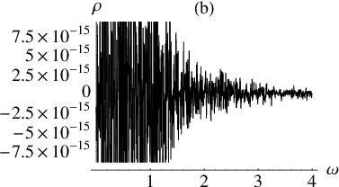
That is, for any particular that we have tried, machine simplification shows the identity of the respective terms in each of these series pairs (but general can’t be handled). Also, numerical plots of the differences of respective partial sums show nothing but numerical noise. (The noise is usually very small (machine-precision level) but not always: The sums over in such formulas as (75) are numerically unstable when is very small. See Fig. 5(b).) On the other hand, partial sums of the three series (89)–(91) are seen to be all different.
When plotted, all the series show, even for very small partial sums, the development of delta peaks at the (square roots of the) eigenvalues of the Robin problem,
| (93) |
In accordance with (85), the periodic terms alone already give the locations of the eigenvalues, and the bounce contributions are needed only to normalize the delta functions correctly. Examples are shown in Fig. 4. For comparison, in the case we computed the lowest-lying eigenvalues by Newton’s method to be
| (94) |
and the large eigenvalues by perturbation theory to be
| (95) |
with which (94) already overlaps well. Fig. 4 agrees well with these values.


We now turn to the issue of what happens for near (Fig. 5). The empirical evidence from the plots is that and , and equivalently and , are behaving exactly as expected: The right-hand half of a delta function is building up at the origin to cancel the (correct, but misleading) in the formulas of Secs. V.5 and V.7. Because of (92), we get the same behavior from and ; that is, the forcible reinterpretation of contributions to the local spectral density from closed but nonperiodic orbits as if they were contributions from periodic orbits has, by the mathematical phenomenon of Appendix A, introduced a truly spurious term into the formulas of Sec. V.6! On the other hand, both and are converging to the right answer for the context of Sec. V.6. Their partial sums differ, but the difference (apparently) goes away in the limit. These series are yielding negative delta functions that precisely cancel the delta behavior of , so that no is ever visible in the total density (see Figs. 5(c,d)).



V.9 Broader implications
This simple one-dimensional model is trivial in comparison with many problems treated by similar methods in the contemporary literature. It cannot manifest quantum chaos; it doesn’t require stationary-phase approximations; it isn’t even relevant to the sort of semiclassical approximation that becomes necessary when a potential is added to the one-dimensional Schrödinger equation (93) lgacee3. Nevertheless, it is instructive. The mere fact that so much information can be obtained exactly means that the model can be understood in complete detail and stands as a benchmark against which partial and approximate solutions of more complicated models can be appraised.
In particular, the delicate problem of the delta function at is likely to have broader implications. In more complicated problems such precise analysis at the bottom end of the spectrum is usually lost in the noise of the semiclassical and stationary-phase approximations. Periodic-orbit reconstructions of spectra are observed to be surprisingly good at low frequencies, except very close to , where a spurious peak often occurs. (Look at Fig. 17 of BB3 and Fig. 29 of FW.) Our analysis suggests that this phenomenon represents not a breakdown of the semiclassical approximation so much as an ambiguity in the ordering of the terms in the badly convergent periodic-orbit sum.
A related point is the significance of contributions from orbits that are closed but not periodic. Usually such contributions are discarded in the process of stationary-phase approximation. However, they are needed to get the boundary terms in BB1; SSCL, and Jaffe and Scardicchio JS; SJ have recently emphasized their importance in calculations of total vacuum energy. As semiclassical calculations are carried beyond the lowest order in , these orbits will need to be included, and one must grapple with the question of whether they must be kept separate, as in (79), or will be effectively absorbed into the periodic contributions as in (75) and (91). In our model they did not influence the location of the eigenvalues, but they were needed for proper normalization; is there some broader significance to that?
Acknowledgements.
We thank Ricardo Estrada, Klaus Kirsten, and Peter Kuchment for helpful remarks. JDB gratefully acknowledges the support of the Advanced Technology Program of the State of Texas, Award 010366-0218-2001 to Robert Kenefick, and we thank Dr. Kenefick for encouraging us to work together.Appendix A Nonabsolute convergence of oscillatory distributions
In the periodic-orbit approach to spectral theory, sums of the type
| (96) |
are often encountered. Typically is a fixed, small number (such as ), and varies slowly with but may become singular as and, most important, does not approach as . Such a series does not converge at all according to the definitions of classical analysis, but nevertheless it may converge in the sense of distributions. The question then arises whether the distributional limit can depend on the order in which the terms are added, in analogy with numerical series that are only conditionally convergent. We consider here distributions defined on the nonnegative real line.
Theorem 5
In (96) assume that is independent of and that the functions are smooth () for and they and all their derivatives are uniformly polynomially bounded as . Then any two orderings of the terms in define distributions that coincide on test functions with support in the interior (i.e., in a neighborhood of the origin). As distributions on test functions defined in they may differ by a distribution supported at (necessarily a linear combination of and its derivatives).
Proof: The definition of distributional convergence is that for any test function ,
| (97) |
converges in the classical sense and defines a continuous linear functional of . If in a neighborhood of the origin, then repeated integration by parts,
shows that each integral in (97) falls off faster than any power of . Taking sufficiently large guarantees that (97) converges absolutely and hence can be reordered at will. If the support of includes the origin, the endpoint terms from the partial integrations may converge to a well-defined delta-type distribution. If not, it may still be possible to extend the distributions to such test functions by “regularization” EF; in that case the coefficients in the delta sum are somewhat ambiguous.
Example: Consider
| (98) |
From one point of view, shifting the index in the first term yields
On the other hand, the th partial sum of (98) as written is
and the latter converges to :
the second term vanishes as by the Riemann–Lebesgue theorem, and the integral in the first term equals (GR, (3.721.1)).
Remark: That the series rearrangements in the body of the paper obey the polynomial boundedness requirement in Theorem 5 follows from the bound (AS, (2.14.13))
| (99) |
on the Laguerre polynomial. Individual terms in (80) (for instance) with can grow exponentially with , but we have never realigned terms with differing values of .
Appendix B Reconstruction of the periodic-orbit sum by Poisson summation
The following is a close analogue of a two-dimensional calculation in Sec. 2.2 of SPSUS. It requires knowledge of the eigenvalue condition (100) (but not of explicit formulas for its solutions).
The square roots of the eigenvalues of the Robin–Dirichlet problem (93) with are the positive roots of
| (100) |
which may be parametrized as
| (101) |
One can view (101) as giving as a function of , which naturally extends to the whole real line as a monotonic and odd function with derivative
| (102) |
Thus is defined for all integers, with and (which is not an eigenvalue). So the eigenvalue density is
| (103) |
References
- (1) Abramowitz M and Stegun I A 1964 Handbook of Mathematical Functions With Formulas, Graphs, and Mathematical Tables (Washington: U S Dept of Commerce)
- (2) Akhiezer N I and Glazman I M 1993 Theory of Linear Operators in Hilbert Space (New York: Dover) app II sec 9
- (3) Balian R and Bloch C 1970 Ann. Phys. (N.Y.) 60 401–447
- (4) Balian R and Bloch C 1972 Ann. Phys. (N.Y.) 69 76–160
- (5) Branson T P and Gilkey P B 1990 Commun. Partial Diff. Eqs. 15 245–272
- (6) Bryan G H 1891 Proc. Camb. Phil. Soc. 7 246–248
- (7) Carslaw H S and Jaeger J C 1959 Conduction of Heat in Solids 2nd ed (Oxford: Clarendon) sec 14.2
- (8) Chen G and Zhou J 1993 Vibration and Damping in Distributed Systems vol I (Boca Raton: CRC) p 1511 1 The title of this book was cited incorrectly in systemat. Also, the citing sentence (p. 6863) should refer to a “localized spring”, not a “point mass”.
- (9) Cohen D, Primack H and Smilansky U 1998 Ann. Phys. (N.Y.) 264 108–170
- (10) de Albuquerque L C and Cavalcanti R M 2004 J. Phys. A: Math. Gen. 37 7039–7050
- (11) Estrada R and Fulling S A 2002 J. Phys. A: Math. Gen. 35 3079–3089
- (12) Estrada R and Fulling S A work in progress
- (13) Friedrich H and Wintgen D 1989 Phys. Rep. 183 37–79
- (14) Fulling S A 1983 J. Phys. A: Math. Gen. 16 2615–2631
- (15) Fulling S A 2003 J. Phys. A: Math. Gen. 36 6857–6873
- (16) Fulling S A 2004 Quantum Field Theory Under the Influence of External Conditions ed K A Milton (Princeton: Rinton) pp 166–174
- (17) Fulling S A work in progress
- (18) Gradshteyn I S and Ryzhik I M 1980 Table of Integrals, Series, and Products (New York: Academic)
- (19) Helson H 1983 Harmonic Analysis (Reading MA: Addison–Wesley) sec 2.4
- (20) Jaffe R L and Scardicchio A 2004 Phys. Rev. Lett. 92 070402
- (21) Kirsten K 1998 Class. Quantum Grav. 15 L5–L12
- (22) Kennedy G, Critchley R and Dowker J S 1980 Ann. Phys. (N.Y.) 125 346–400
- (23) Romeo A and Saharian A A 2002 J. Phys. A: Math. Gen. 35 1297–1320
- (24) Scardicchio A and Jaffe R L 2004 preprint quant-ph/0406041
- (25) Sieber M, Primack H, Smilansky U, Ussishkin I and Schanz H 1995 J. Phys. A: Math. Gen. 28 5041–5078
- (26) Sieber M, Smilansky U, Creagh S C and Littlejohn R G 1993 J. Phys. A: Math. Gen. 26 6217–6230
- (27) Stakgold I 1979 Green’s Functions and Boundary Value Problems (New York: Wiley) ch 7 exercise 3.2
- (28) Tikhonov A N and Samarsky A A 1953 Uravneniya Matematichesckoy Fiziki (Moscow: GITTL) [Tychonov A N and Samarski A A 1964 Partial Differential Equations of Mathematical Physics (San Francisco: Holden–Day)] secs II.1.7 and II.2.7
- (29) Wolfram S 1999 The Mathematica Book 4th ed (Cambridge: Cambridge)