Invariant and Group Theoretical Integrations over the $U(n)$ Group

The invariant method presented in a previous paper [8] can be used to calculate the integral (1). The method exploits the unitarity of the $U(n)$ group elements,

and the invariance of the Haar measure, in the form

for any function $f$ and any $V\in U(n)$.

The unitarity relation (4) relates integrals of the same degree if $i\not=l$, and it relates integrals of degree $p$ to integrals of degree $p-1$ if $i=l$. Other relations between integrals of the same degree can be obtained from (5), by suitable choices of $V$. Here are some of them discussed in the previous paper [8].

1. 1.

   Using $V_{ij}=e^{i\phi}\delta_{ij}$, it follows that $p$ must be equal to $q$ in order to avoid the vanishing of integral (2). The number $p$ will be called the degree of the integral.

2. 2.

   Using $V_{ij}=e^{i\phi_{i}}\delta_{ij}$, it follows that (2) is nonzero only when $K=I_{M}$ and $L=J_{R}$ for some $M,R\in S_{p}$. Using (3), and denoting $RM^{-1}$ by $Q$, only integrals of the type

   $$\langle IJ|IJ_{Q}\rangle=\int(dU)\,U_{IJ}^{*}\,U_{IJ_{Q}}$$

   (6)

   are nonzero, so from now on we need to consider only integrals of this type.

   An integral with $J_{Q}=J$ will be called a direct integral. For such integrals we may always choose $Q=e$, the identity permutation. Otherwise, the integral is an exchange integral.

   Integrals are represented diagrammatically as follows. Each distinct value in the index set $I$ is represented by a dot on the left (L-dot), and each distinct value of the index set $J$ or $J_{Q}$ is represented by a dot on the right (R-dot). The factor $U^{*}_{ij}$ is shown as a thin solid line between the L-dot $i$ and the R-dot $j$, and the factor $U_{ij}$ is shown as a dotted line between these two dots. The factor $U^{*}_{ij}U_{ij}$ is represented by a thick line, or more generally, the factor ${U^{*}}_{ij}^{m}U_{ij}^{n}$ is represented by a thick line with a pair of numbers $(m,n)$ written beside it. If $m=n$, then only a single number $m$ is written. The numbers $(m,n)$ or $m$ will be known as the multiplicities of the line. See Fig. 1 for an illustration.

   

3. 3.

   With $V$ chosen to be a permutation matrix of n objects, it follows that

   $$\langle IJ|KL\rangle=\langle I^{\prime}J|K^{\prime}L\rangle=\langle IJ^{\prime}|KL^{\prime}\rangle,$$

   where $I^{\prime}$ is obtained from $I$ by a reassignment of the values of its indices, e.g. if $I=(334)$, then $I^{\prime}$ may be $(558)$. $K^{\prime}$ is obtained from $K$ by the same reassignment, and similarly for $J^{\prime}$ and $L^{\prime}$. As a result, there is no need to know the values of the indices of the L-dots, nor the R-dots. This is why the dots in Fig. 1 are not labelled.

4. 4.

   As a consequence of the first two equalities in (5), an integral remains the same under the interchange of the solid lines with the dotted lines, or the L-dots with the R-dots.

5. 5.

   Using $V=R(ab)$, the rotation matrix in the $(a,b)$ plane, a ‘spin-off relation’ is obtained. Consider a R-dot imbedded in an arbitrary integral $M_{0}=\langle IJ|IJ_{Q}\rangle$, with $d$ pairs of solid-dotted lines attached to the dot. Now spin off $e$ pairs of these lines to create a new R-dot and a new integral. There are many ways to choose the $e$ pair of lines, each possibly corresponds to a different integral. Let $M_{e}$ be the sum of all these integrals. Then the quantities $M_{0}$ and $M_{e}$ are related by the spin-off relation

   $$M_{e}=M_{0}\,\left(\!\!\begin{array}[]{c}d\\ e\end{array}\!\!\right),$$

   (7)

   where $\left(\!\!\begin{array}[]{c}d\\ e\end{array}\!\!\right)$ is the binomial coefficient.

   The relation is local in that it is independent of the the structure of the rest of the diagram. The same relation can also be used to spin off a L-dot.

In what follows, we summarize two general results obtained in the previous paper [8] using the IM.

The fan relation can be generalized to a double-fan relation, connecting the closed ‘double-fan’ diagram of Fig. 3(a) with a (fully) opened double-fan diagram such as Fig. 3(b). As in Fig. 2, there may be additional dots and lines in the integral, but none of them may end up on the R-dots shown. From that relation, we can also deduce relations between a closed double-fan and a partially opened double-fan, as done in the single-fan case.

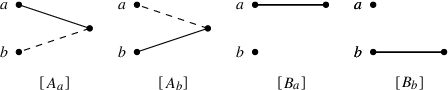
The double-fan relation is considerably more complicated than the single-fan relation (8), because there are many more double-fan graphs. Each R-dot of a (fully) opened (double-fan) graph such as Fig. 3(b) falls into one of four basic patterns: $[A_{a}],[A_{b}],[B_{a}]$, and $[B_{b}]$, shown in Fig. 4. If the solid and dotted lines end up on the same L-dot, the pattern is a $[B]$; otherwise it is an $[A]$. The subscripts $a$ and $b$ tell us which L-dot the solid line emerges from.

Suppose there are $\alpha_{i}$ number of $[A_{i}]$ and $\beta_{i}$ number of $[B_{i}]$ patterns in a (fully) opened (double-fan) graph. Then there are $m_{a}$ solid and $n_{a}$ dotted lines emerging from the L-dot $a$, and $m_{b}$ solid and $n_{b}$ dotted lines emerging from the L-dot $b$, where

The total number of R-dots in the opened graph is $N=m_{a}+m_{b}=n_{a}+n_{b}$.

When these $N$ R-dots are merged together, we get the closed (double-fan) graph depicted in Fig. 3(a), which will be denoted by $[(m_{a}n_{a})(m_{b}n_{b})]$. If $N=1$, this is just one of the four basic patterns discussed before. If $N>1$, we will call it a compound pattern.

From (11), we see that if we replace $\alpha_{i}$ and $\beta_{i}$ by $\alpha_{i}^{\prime}=\alpha_{i}+\xi$ and $\beta_{i}^{\prime}=\beta_{i}-\xi$, with any integral $\xi$ which keeps $\alpha_{i}^{\prime}$ and $\beta_{i}^{\prime}$ nonnegative, then we get the same closed graph by collapsing this new opened graph. Conversely, it will be shown in Appendix A that the closed graph $[(m_{a}n_{a})(m_{b}n_{b})]$ can be spinned off into a sum of several opened graphs, one for each $(\alpha_{i}^{\prime},\beta_{i}^{\prime})$. The double-fan relation expressing that quantitatively is

where

and the sum is over all solutions $(\alpha_{a}^{\prime},\alpha_{b}^{\prime},\beta_{a}^{\prime},\beta_{b}^{\prime})$ of (11).

The double fan becomes a single fan if the L-dot $b$ is not connected, namely, if $m_{b}=n_{b}=0$ and $m_{a}=n_{a}\equiv m$. In that case (12) becomes

which is just (8) (when all $m_{i}=1$) in another notation.

Using group theory, the integral (6) can be turned into a multiple sum [5, 6]. In the notation used in Appendix A of [8], the formula is

where $p$ is the degree of the integral. The symbols ${\cal G}_{I}$ and ${\cal G}_{J}$ represent the symmetry groups of the row and column index sets. More precisely, ${\cal G}_{X}=\{P\in S_{p}|P(X)=X\}$, with $X$ being either $I$ or $J$. The irreducible representations of the symmetric and unitary groups are both labelled by a sequence $f=(f_{1},f_{2},\ldots,f_{p})$, with $f_{1}\geq f_{2}\geq\cdots\geq f_{p}\geq 0$. $\chi_{f}(P)$ is the character of $P\in S_{p}$ in the irreducible representation with signature $f$. The dimension of the irreducible representation $f$ is given by $d_{f}=\chi_{f}(e)$ for $S_{p}$, and by $\tilde{d}_{f}$ for $U(n)$. A formula for $\tilde{d}_{f}$ is:

where $D(x_{1},\ldots,x_{n})$ is the Vandermonde determinant given by $\prod_{i<k}(x_{i}-x_{k}).$

Since $\chi_{f}(g)$ depends only on the class $c_{g}$ that $g$ belongs to, we may write it as $\chi_{f}(c_{g})$. With this notation, eq. (14) can be re-written as

where the sum is taken over all classes $c$ of $S_{p}$,

is the number of elements of the type $SQR$ in the class $c$, and

It is not difficult to see that $Q$ is not unique, because $Q^{\prime}=SQ=QT$ for any $S\in{\cal G}_{J}$ and any $T\in{\cal G}_{J_{Q}}$ is another possible $Q$. It does not matter which $Q$ we pick in (17). That equation can also be written as

It is straightforward but generally very tedious to compute $N[c]$, because we need to calculate the product $QTR$ for every $T\in{\cal G}_{J_{Q}}$, every $R\in{\cal G}_{I}$, and determine what class $c$ the product belongs to. Then we have to count up all the products that are in a given class $c$ to get $N[c]$. However, the task becomes considerably more manageable if either ${\cal G}_{I}$ and ${\cal G}_{J_{Q}}$ are disjoint, or if one is contained in the other. We shall refer to integrals with those properties as orderly. Further simplification occurs for direct integrals, because in that case $Q$ can always be chosen to be the identity $e$, so the triple product is reduced to a double product $TR$.

The calculation of $\xi[c]$ in (18) is simpler than the calculation of $N[c]$, but still we know of no closed form of it valid for every class $c$ and every symmetric group $S_{p}$. The best we can do is to compute them case by case. Results are given in Sec. 3.3. Each $\xi[c]$ is actually an orderly integral with ${\cal G}_{I}={\cal G}_{J}=e$, to be referred to as a primitive integral.

Other integrals can be computed in terms of the primitive integrals, if $N[c]$ is known. We shall discuss two orderly integrals for which $N[c]$ can easily be obtained. In Sec. 3.4, we discuss the stack integrals, which are direct integrals with ${\cal G}_{I}={\cal G}_{J}$. In Sec. 3.5, we discuss the fully opened double-fan integrals of the type $[A_{a}]^{\alpha}[A_{b}]^{\alpha}$.

Relations between orderly integrals may be obtained without knowing the explicit values of $\xi[c]$, if their $N[c]$’s are related in a simple way. This is the case for the single-fan relation, and the double-fan relation with $n_{a}=m_{b}=0$ and $m_{a}=n_{b}=m$. They will be discussed in Sec. 3.2. However, general double-fan integrals are not orderly, so we cannot obtain the general double-fan relation by the group-theoretical method, at least not in the present way. We will also show that the closed (single-)fan integral can also be computed without explicitly knowing what $\xi[c]$ are. This is one of the very few cases where integrals can be obtained group-theoretically without explicitly knowing $\xi[c]$.

That leaves the non-orderly integrals, for which each term of the summand in (19) has to be calculated separately to get $N[c]$. The first non-orderly integral occurs in degree $p=3$. In Sec. 3.6, we shall show how to calculate some of the $p=3$ and $p=4$ non-orderly integrals.

The single-fan integrals are orderly. The index sets for the closed fan Fig. 2(a) are

The first row gives the index labels, and the next three rows give the values of the indices in the sets $I,J,$ and $J_{Q}$ respectively. Different letters are understood to correspond to different values. Additional dots and lines may be present in the graph, as long as none of the lines end up in the R-dots shown. These additional lines and dots are not drawn because they do not affect the fan relation in any way. Similarly, they are not shown in the index sets in (20) other than the ellipses in the first two rows, which remind us that there may be more lines connected to the L-dots. Such ellipses are absent in the last two rows because no additional lines are allowed to be connected to the R-dots shown.

Similarly, the index sets for the fully opened fan, Fig. 2(b) with all $m_{i}=1$, are

Using $S_{m}$ to denote the symmetric group for the permutation of the first $m$ labels, the symmetric groups for Fig. 2(a) can be read off from (20) to be ${\cal G}_{I}\supset S_{m}$ and ${\cal G}_{J}={\cal G}_{J_{Q}}=S_{m}$. Similarly, the symmetric groups for Fig. 2(b) can be read off from (21) to be ${\cal G}_{I}\supset S_{m}$ and ${\cal G}_{J}={\cal G}_{J_{Q}}=e$. We may choose $Q=e$ in both cases. Then for Fig. 2(a), $T{\cal G}_{I}={\cal G}_{I}$ for every $T\in{\cal G}_{J_{Q}}$, hence $N[c]=m!\sum_{R\in{\cal G}_{I}}\delta(R\in c)$. But the last sum is simply the $N[c]$ for Fig. 2(b) and (21). Hence it follows from (16) that the fan relation (with all $m_{i}=1$) is true.

Next, let us derive the double-fan relation (12) and (13) for the case $n_{a}=m_{b}=0$ and $m_{a}=n_{b}$. The solution of (11) is now unique. It gives $\alpha_{a}=m_{a}=n_{b}\equiv m$, and $\alpha_{b}=\beta_{a}=\beta_{b}=0$. The double-fan relation (12) then becomes

The closed double-fan is shown in Fig. 5(a). Its index sets are

The opened double-fan is shown in Fig. 5(b). Its index sets are

We may choose $Q=(1,n)(2,n+1)\cdots(m,n+m)$ in both cases. For (23), ${\cal G}_{I}\supset S_{m}\otimes S^{\prime}_{m},{\cal G}_{J}=S_{m}$, and ${\cal G}_{J_{Q}}=S^{\prime}_{m}$, where $S_{m}$ is the permutation group of the first $m$ labels, and $S_{m}^{\prime}$ is the permutation group for the labels $(n,n+1,\cdots,n+m)$. For (24), ${\cal G}_{I}\supset S_{m}\otimes S^{\prime}_{m}$, but ${\cal G}_{J}={\cal G}_{J_{Q}}=e$.

For Fig. 5(a), $T{\cal G}_{I}={\cal G}_{I}$ for every $T\in{\cal G}_{J_{Q}}$. Hence $N[c]=m!\sum_{T\in{\cal G}_{I}}\delta(QR\in c)$. But the last sum is simply the $N[c]$ of Fig. 5(b). In this way (22) is proven by the GTM.

The fan integral (10) can also be obtained from the GTM. It is given by Fig. 2(a) without extra dots and lines, or (20) without the ellipses at the end. Then ${\cal G}_{I}=S_{m}$, and $N[c]=m!\sum_{R}\delta(R\in c)$. From (16) and (18), we get

In getting from (25) to (26), the character $\chi_{(m)}^{\ast}(R)=1$ of the totally symmetric representation $(m)$ of the permutation group has been inserted, and the orthogonality relation of the characters has been used. To get to (27), $d_{(m)}=\chi_{(m)}(e)=1$ as well as $\tilde{d}_{(m)}=(m+n-1)!/(n-1)!m!$ (see (15)) have been used.

The result in (27) agrees with the result (10). It is one of the very few cases where the value of the integrals can be obtained group-theoretically without knowing the values of the individual $\xi[c]$’s.

Integrals in which both symmetry groups ${\cal G}_{I}$ and ${\cal G}_{J}$ consist only of the identity $e$ will be called primitive. This happens when all the indices $i_{a}$ in the set $I$ assume distinct values, and all the indices $j_{b}$ in the set $J$ are also different. The corresponding diagrams have $p$ dots each on both columns, and precisely one solid and one dotted lines connecting to each of the dots. The primitive diagrams for $p\leq 3$ are shown in Fig. 6, and the ones for $p=4,5$ are contained in Appendix C.

Since ${\cal G}_{I}={\cal G}_{J}=e$, it follows from (17) that $N[c]=\delta(Q\in c)$, where $Q$ can be any element of $S_{p}$. The primitive integrals (16) are simply $\xi[c]$, one for each class $c$ of $S_{p}$. We may therefore use an element of each cycle structure to label the primitive integrals, as is done in Fig. 6. Diagrammatically, the cycle structure is translated into the loop structure of its diagram, as can be seen in Fig. 6. Using (18) along with (15) and the character tables found in Appendix B (note that $d_{f}=\chi_{f}(e)$), the primitive integrals for $p\leq 3$ can be easily computed, and the results are displayed in Table 1. The results for $p=4,5$ can also be found in Table 4 of Appendix C.

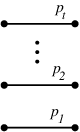
The stack diagrams (see Fig. 7) are direct integrals made up of disconnected lines of arbitrary multiplicities. As such, $Q=e$, and $J$ differs from $I$ only by relabelling. Using item 3 of Sec. 2.2, we may assume $J=I$. Hence stack integrals are integrals of the form $\langle II|II\rangle$.

Let $p_{1},p_{2},\ldots,p_{t}$ be the multiplicities of the disconnected lines in a stack diagram. Then ${\cal G}_{I}={\cal G}_{J}\equiv{\cal G}=S_{p_{1}}\otimes S_{p_{2}}\otimes\cdots\otimes S_{p_{t}}$, and $N[c]$ is nonzero only when the class $c$ is a direct product of the classes $c_{i}$ of the groups $S_{p_{i}}$. In that case,

where $n_{i}(c_{i})$ is the number of elements of $S_{p_{i}}$ in the class $c_{i}$. In other words,

where the class $c_{i}$ consists of $\alpha_{j}$ cycles of length $j$. Denoting the stack integral $\langle II|II\rangle$ by $\Xi(p_{1},p_{2},\ldots,p_{t})$, we get

All stack diagrams can be obtained by making the assignment $f_{i}\rightarrow p_{i}$ from each representation. In this way, we expect a same number of stack digrams as of primitive diagrams, or classes. Using the $\xi$ expressions obtained in the preceding subsection, the stack integrals for $p\leq 3$ can be computed to yield the expressions in Table 2.

The index sets for the fully opened double-fan integrals $[A_{a}]^{\alpha}[A_{b}]^{\alpha}$ (Fig. 3(b) with $N=2\alpha$) are

Hence both ${\cal G}_{J}$ and ${\cal G}_{J_{Q}}$ consist only of the identity $e$. As for ${\cal G}_{I}$, it is given by $S_{\alpha}\otimes S_{\alpha}$, where the permutation groups $S_{\alpha}$ act respectively on the $b$ and $a$ indices in $I$. The element $Q$ maps $J_{Q}$ to $J$, i.e. $Q=(1,\alpha+1)(2,\alpha+2)\cdots(\alpha,2\alpha)$.

The fully opened integral can be computed using (16), with $N[c]$ given by (17) or (19). Thus,

where the last sum is over every permutation $Q^{\prime}$ that sends all $b$ indices in (31) to the positions labelled from $\alpha+1$ to $2\alpha$, and similarly all $a$ indices to the positions labelled from $1$ to $\alpha$. As a consequence, the allowed cycles of $Q^{\prime}$ must be of even length, and they can be specified by a sequence of nonnegative integers $(k)\equiv(k_{1}k_{2}\cdots k_{\alpha})$, $k_{i}$ being the number of cycles of length $2i$. The number of $Q^{\prime}$ with the class structure $(k)$ that is related to $c$ is given by

In order to see how this is arrived at, consider an example where $k_{1}=2$, $k_{2}=2$, and all other $k_{i}$ values are zero. Then $Q^{\prime}$ is of the form ($ba$)($ba$)($baba$)($baba$), where the $b$ and $a$ letters should take the distinct index labels in $(1,\ldots,\alpha)$ and $(\alpha+1,\ldots,2\alpha)$ respectively. Another $Q^{\prime}$ with the same cycle structure can thus be obtained by permuting individually all the $a$ and $b$ labels. This accounts for the numerator in (33). However, such permutations do not necessarily give distinct $Q^{\prime}$ elements. The cyclic nature of a cycle tells us that each cycle of length $2i$ will appear $i$ times; this accouts for the $i^{k_{i}}$ factor in the denominator. Moreover, no new $Q^{\prime}$ is obtained if we permute cycles of the same length; that accounts for the other factor $k_{i}!$ in the denominator.

We may now return to (16) to calculate the integral $[A_{a}]^{\alpha}[A_{b}]^{\alpha}$ in terms of the primitive integrals $\xi[c]$. The result for the first few $\alpha$ values are listed in Table 3.

All integrals with degree $p<3$ are orderly. The non-orderly integrals of $p=3$ are shown in Fig. 8, and those related to them by the fan relation (8). The calculation of $N[c]$ and the integral for each of them is discussed below. The integrals will be labelled by their figure, e.g., integral $I(\ref{fig:diag3c}a)$.

The index sets for Fig. 8(a) are

They give rise to the symmetry groups ${\cal G}_{I}=\{e,(12)\}$ and ${\cal G}_{J}={\cal G}_{J_{Q}}=\{e,(23)\}$. Moreover, the element $Q$ can be taken to be the identity element. In order to obtain the coefficients $N[c]$ of equation (16), we need to compute $QTR$ for all $T\in{\cal G}_{J_{Q}}$ and $R\in{\cal G}_{I}$. That triple product is $Q{\cal G}_{J_{Q}}{\cal G}_{I}=\{e,(12),(23),(132)\}$. As a result,

In the same way, the index sets of Fig. 8(b) are

and hence the symmetry groups are ${\cal G}_{J_{Q}}=\{e\}$ and ${\cal G}_{I}=\{e,(23)\}$, and the exchange element is $Q=(12)$. We thus obtain $Q{\cal G}_{J_{Q}}{\cal G}_{I}=\{(12),(123)\}$, from which

follows.

Finally, for Fig. 8(c), the index sets are

The relevant symmetry groups are ${\cal G}_{J_{Q}}=\{e,(13)\}$ and ${\cal G}_{I}=\{e,(23)\}$. With $Q=(12)$, the set $Q{\cal G}_{J_{Q}}{\cal G}_{I}$ is $\{(12),(13),(123),(132)\}$, and formula (16) gives:

References

- [1] P. Di Francesco, P. Ginsparg, and J. Zinn-Justin, Phys. Rep. 254, 1 (1995); S.L. Shatashvili, Comm. Math. Phys. 154, 421 (1993); A. Morozov, Mod. Phys. Lett. A7, 3503 (1992).
- [2] A. Mueller-Groeling, and H.A. Weidenmueller, Phys. Rep. 299, 189 (1998) [cond-mat/9707301].
- [3] G. Mahlon, C.S. Lam, and W. Zhu, Phys. Rev. D66, 074005 (2002).
- [4] M. Creutz, J. Math. Phys. 19, 2043 (1978).
- [5] C. Itzykson and J.-B. Zuber, J. Math. Phys. 21, 411 (1980).
- [6] S. Samuel, J. Math. Phys. 21, 2695 (1980); I. Bars, J. Math. Phys. 21 (1980) 2678; I. Bars, Phys. Scripta 23, 983 (1981); A. Morozov Mod. Phys. Lett. A7, 3503 (1992); A.B. Balantekin, Phys. Rev. D62, 085017 (2000); B. Collins, math-ph/0205010; B. Schlittgen and T. Wettig, J. Phys. A36, 3195 (2003); P. Zinn-Justin and J.-B. Zuber, J. Phys. A36, 3173 (2003).
- [7] H. Weyl, ‘The Classical Groups’, (Princeton University Press, 1966).
- [8] S. Aubert and C. S. Lam, J. Math. Phys. 44, 6112 (2003). [math-ph/0307012].
- [9] M. Hamermesh, “Group Theory and its Application to Physical Problems”, (Dover, 1962).