Dynamics of lumps on a cylinder
Abstract
The slow dynamics of topological solitons in the -model, known as lumps, can be approximated by the geodesic flow of the metric on certain moduli spaces of holomorphic maps. In the present work, we consider the dynamics of lumps on an infinite flat cylinder, and we show that in this case the approximation can be formulated naturally in terms of regular Kähler metrics. We prove that these metrics are incomplete exactly in the multilump (interacting) case. The metric for two-lumps can be computed in closed form on certain totally geodesic submanifolds using elliptic integrals; particular geodesics are determined and discussed in terms of the dynamics of interacting lumps.
1 Introduction
Many field theories possess topological solitons as classical solutions, and the study of their dynamics has long been an important research topic in mathematical physics. Exact results for this problem have only been obtained for rather special (integrable) models in dimensions; more generally, one has to resort to approximations based on truncations of the field theories to finite-dimensional configuration spaces of collective coordinates. One such scheme is the adiabatic approximation, first proposed by Manton in the context of BPS monopoles [1]. It has been applied to extract detailed information about the slow dynamics of solitons in a number of models in , and more dimensions (notably gauged Ginzburg–Landau vortices [2, 3] and Yang–Mills–Higgs monopoles [4, 5]) and is believed to work well for a large class of field theories exhibiting self-duality.
One neat example of a self-dual field theory is the nonlinear -model with target on a Riemann surface . This is the dynamical system for maps
described by the wave equation associated to a specific riemannian metric on and the usual round metric on the two-sphere . Topological solitons in this model, usually referred to as lumps, will typically arise if is compact or effectively compactified by suitable boundary conditions. Static solutions are harmonic maps, with energy given by the usual Dirichlet integral. In the adiabatic approximation, one constructs another dynamical system whose configuration space consists of the static solutions of minimal energy, the dynamics being defined by restricting the action functional of the original field theory. This space is stratified by homotopy classes, and the strata are usually referred to as the moduli spaces. For the -model, the Dirichlet energy is minimized exactly by the holomorphic or antiholomorphic maps within each homotopy class, labelled by the Brouwer degree of . The moduli spaces (if non-empty) then have the structure of finite-dimensional complex varieties [6], and the adiabatic dynamics is geodesic motion with respect to a metric on them. The Cauchy–Riemann equation, a first-order PDE, replaces the second-order static equations of motion as a description of the fields. This is the essential common feature to all self-dual theories. In the adiabatic programme, the moduli spaces are often smooth manifolds equipped with natural geometric structures (symplectic forms, metrics of special holonomy) that turn out to be interesting objects by themselves. In some instances, they have even been used to probe aspects of the quantum field theories underlying the original models [7, 8, 9].
The -model has applications to the physics of ferromagnets and as a high-energy effective model for vortices; however, its main interest has been as a toy-model displaying many of the features of more important field theories with gauge symmetry. The adiabatic approach to this model was first investigated by Ward for the case in [10]; he found that the approximation is ill-defined, in the sense that the metric is infinite along certain directions that appear as frozen degrees of freedom. One way to regularise the metric is to place the vortices on a compact surface, and this was studied by Speight when is a sphere [11] or a torus [12]. It has also been found that the metric for regularises once a self-gravitating interaction is included in the lagrangian [13]. Determining these metrics in closed form is in general beyond reach, but some explicit formulae have been obtained in a number of nontrivial cases, namely for one-lumps on [11] and for certain totally geodesic submanifolds of two-lumps on [10] and on the particular torus [12]. Geodesic incompleteness of the moduli spaces was proved in [14]. There is also a general belief that the relevant metrics should be Kähler [15, 16]; this has been rigorised for , and for and [17]. The accuracy of the adiabatic approximation has been studied recently by Haskins and Speight [18] in the spirit of work by Stuart [3, 5] on the gauge theory models.
In this paper, the adiabatic dynamics of lumps is studied in some detail for the case where is an infinite cylinder. We can say that this is an intermediate case between the situations and compact considered by previous authors. In the former, the metrics are ill-defined but explicit calculations of the metric are possible, whereas in the latter the metrics are regular but extremely hard to compute; the cylinder turns out to combine the advantages of both. So our study complements the existing literature in a setting that is unifying in some way, and our results will reflect this. Let us summarise how this paper is organised. We use the next section to fix the basic notation. In section 3, we obtain elementary properties of the moduli spaces; we formulate the adiabatic approximation in terms of regular riemannian metrics, which are shown to be Kähler. In section 4, we discuss the isometries of these metrics. The one-lump sector is studied in section 5. We then establish that all the multilump metrics are incomplete in section 6. In section 7, we address the two-lump dynamics and derive more explicit results about the metric, its geodesics and curvature properties. Finally, we discuss our results in section 8.
2 The -model on a cylinder
For the rest of the paper, we shall take to be the infinite cylinder
with local complex coordinates and metric
| (1) |
induced from the euclidean metric of its universal cover .
The action for the -model, whose objects are differentiable maps dependent on time , is given by
| (2) |
with kinetic and potential energies
| (3) | |||||
| (4) |
We shall only consider the dynamics of maps for which the potential energy above is finite. We represent by means of an inhomogeneous coordinate taking values in following usual practice; overdots denote time derivatives and is the measure on associated to (1). The variational principle yields the wave equation as equation of motion, and static solutions are harmonic maps from to . Here, is the riemannian metric on regarded as a two-sphere of unit radius; the Kähler -form of this metric will be denoted by . Following an argument first presented by Belavin and Polyakov [19] (but already observed in a more general setting in the mathematical literature — cf. [20] p. 374), we write for a map
where is the Brouwer degree of the map. In the inequality above, it is useful to take the top signs if is nonnegative, and the bottom signs otherwise. Then we learn that
which implies that provided is finite. Moreover, we deduce that the potential (or Dirichlet) energy (4) is minimized to on each topological class by a solution of the Cauchy–Riemann equation
| (5) |
if , or if . To simplify our discussion, we will mostly be considering the case only, but all the statements can be easily adapted to the case.
In this paper, we shall be concerned exclusively with the adiabatic approximation to the dynamics (2). This takes place in the space of holomorphic maps from to , i.e. meromorphic functions on . They are completely characterised by the following lemma.
Lemma 2.1.
Any meromorphic function of degree factorises uniquely as
where is given by and is a rational map of degree .
Proof.
Any meromorphic map on can be regarded as a meromorphic map on of period . We first claim that there is a unique meromorphic map such that . This is true because is invertible in modulo integer multiples of , and this ambiguity does not change the value of ; that is meromorphic (and thus a rational map) follows from being holomorphic and the inverse function theorem in one complex variable. Since has degree one and the degree is multiplicative with respect to composition, has degree . Finally, can be extended to a meromorphic map in a unique way: it cannot have essential singularities at or , for then the (strong version of the) big Picard theorem (cf. [21] p. 210) would contradict . ∎
A meromorphic (or antimeromophic) map on of degree will be called an -lump. Lumps with are sometimes called antilumps.
Corollary 2.2.
For any lump , the limits
are well defined as points of the Riemann sphere.
Proof.
The map determined from by Lemma 2.1 is continuous, so this follows from the existence of and . ∎
We shall call and the endpoints of . It is easy to see that the existence of endpoints is a necessary condition for the Dirichlet energy (4) of any map to be finite.
Remark 2.3.
Lumps with can be interpreted as meromorphic functions on the pinched torus depicted in Figure 1 — an elliptic curve with a nodal singularity and flat metric (1). So the results that we shall obtain below for such maps can also be interpreted in the context of the -model defined on this singular space.

3 Moduli spaces of lumps
The moduli space of -lumps will be denoted by . By Lemma 2.1, any can be written as
| (6) |
where
| (7) |
are complex polynomials with no common roots, and such that and are not both equal to zero. These conditions are expressed algebraically by the nonvanishing of the resultant of and ,
| (8) |
Notice that the polynomials and are not uniquely determined from , but subject to the ambiguity of simultaneous multiplication by an element of . Thus we can regard as a subset of through the injection that maps an -lump given by (6)–(7) to the point
The image of this map is the complement of the hypersurface of degree associated to the homogeneous polynomial in (8),
and is therefore an open subset in the Zariski topology of . So we have shown:
Proposition 3.1.
is a smooth complex quasiprojective variety of dimension
Let denote the diagonal in . For our purposes, it will be useful to give the following description of the moduli spaces:
Proposition 3.2.
There exists a morphism for
| (9) |
whereby associates to each lump its endpoints; for , this is a fibration by smooth irreducible closed subvarieties of with complex dimension . Moreover, is an algebraic principal fibre bundle with structure group .
Proof.
We define as the restriction of the rational map given by
| (10) |
On the complement of the hypersurface , and are never equal to ; thus (10) is regular on , and is a morphism of algebraic varieties.
The fibre of over is obtained by intersecting with the algebraic subset of defined by the homogeneous polynomials
Since these polynomials are linear in different variables and nonzero, it is clear that
is isomorphic to the ring of complex polynomials in variables, whose homogeneous maximal spectrum is . If , it straightforward to verify that this intersects transversely independently of , and this shows that all the fibres are irreducible, smooth and of dimension .
For , it is easily checked that belongs to the ideal
exactly when , so that the range of in this case is the complement of the diagonal . To show that is a principal fibre bundle, we start by pointing out that the identification of one-lumps with rational maps of degree one given by Lemma 2.1 endows with an algebraic group structure, namely
More precisely, we identify one-lumps with Möbius transformations of . The subgroup generated by rotations and dilations is isomorphic to , and it is an easy task to verify that the quotient map
can be identified with . ∎
The pre-image of under the map considered in Proposition 3.2 will be denoted by ; we shall also write . The adiabatic approximation consists of endowing each of these spaces with a riemannian metric and studying its geodesic flow, which is a dynamical system on by automorphisms of the fibration . The geodesics on the fibres can be interpreted physically as a slow motion of lumps of degree preserving the endpoints labelling the fibre. Physically, it makes sense to constrain the motion of the endpoints because we know that in the model it costs an infinite amount of energy to move them, which is not available to a lump that starts moving with a finite velocity.
The metric on each is obtained from the kinetic energy (3) of the -model. This means that, if () are local complex coordinates for , is defined such that
| (11) |
Here we allow the , regarded as parameters specifying , to depend on time and apply the chain rule. Geometrically, can be interpreted as the restriction of the metric on the infinite-dimensional manifold of smooth maps to a finite-dimensional submanifold of holomorphic maps with suitable boundary conditions. Thus given and two vectors of the tangent space
the metric at is evaluated as
| (12) |
whenever this integral exists. The main result of this section is the following
Theorem 3.3.
The riemannian metric on relevant for the adiabatic approximation is regular for . Moreover, it is a Kähler metric with respect to the complex structure induced by .
Proof.
Since we still have the freedom of choosing the inhomogeneous coordinate on the target, we may assume without loss of generality that . This means that we can restrict our attention to maps for which . This condition defines an affine piece of where
| (13) |
are good complex coordinates. Now implies on . There is one more redundant coordinate on among (13), and it can be eliminated through the equation
| (14) |
where . Suppose first that holds, so that can be eliminated. Then a map can be expressed as
| (15) |
where we write . (If , the sum in the numerator should be ignored and .) According to (11), the components of the metric in these coordinates can be read off as
| (16) | |||||
where the indices run from to and we have used the change of variables . After differentiating (15), it is not hard to check that the integrand in (16) (with respect to the euclidean measure ) is a rational function of and , with the only singularity occurring at and being of the form as , and with the asymptotic behaviour as . So we conclude that the integral in (16) is finite for all and , which means that the metric is regular.
To show that the metric is Kähler, we start by observing that it is hermitian with respect to the complex structure associated to the coordinates ,
The closure of the corresponding -form can then be seen to be equivalent to the conditions
For these to hold, it is sufficient that integration and differentiation with respect to may be interchanged in But this follows from a standard result on Lebesgue integration of differentiable maps (cf. e.g. [22], p. 226) once we observe that the integral
exists and is finite by an argument analogous to the one used to establish regularity of .
It remains to address the case , i.e. . Then we necessarily have and (14) yields . A map is now expressed as
| (17) |
(where the sum in the denominator should be ignored if ). The rest of the argument follows essentially unchanged from the case above. ∎
4 Isometries of
Our major goal is to compute explicitly the metrics describing the slow motion of lumps in some special situations and interpret their geodesics. Not surprisingly, a central part of this study is concerned with the exploration of isometries, to which we shall now turn. In this section, will not necessarily be taken as nonnegative.
Recall that is determined from both the metric on space and the metric on the target, cf. (12). These have isometry groups
| (18) |
and
where denotes the Vierergruppe . They act on these spaces as follows. The factor of refers to the translation group of the cylinder,
whereas the Vierergruppe is generated by any two of the three transformations
| (19) | |||||
| (20) | |||||
| (21) |
which also define the semidirect product in (18). Notice that both and reverse the orientation of , whereas preserves the orientation. On the target, the proper rotations in can be represented in terms of Möbius transformations of the coordinate by
| (22) |
and we can take a reflection across any great circle as the generator of the factor, say
It is natural to expect isometries of to be produced from the induced action of on :
In general, these transformations do not preserve the spaces , but it is straightforward to show from the representation (12) that they still act isometrically as follows:
The next proposition shows how these isometries can be used to simplify the study of the metrics .
Proposition 4.1.
Each fibre of is isometric to a fibre of the form with . Moreover, the isometry groups of these spaces always contain a subgroup isomorphic to
if , contains a subgroup isomorphic to if or .
Proof.
Consider the fibre of over arbitrary . If , we can use to map it isometrically to . If , we then use the transformation
(to be read as if ) to map it to a fibre of the form . Finally, if , we use a rotation by . The composition of these isometries then takes to for some .
To prove the second part, we start by recalling from above that the translations of preserve each , so that . This is not the case for the transformations induced by the generators of , but they can be combined with target transformations to produce from the in (19)–(21). Specifically, we take
| (23) | |||||
| (24) |
where is defined by
| (25) |
It is clear that the proper rotations of the target giving rise to isometries of must fix the set , so they are either in (25) (leading to above) or an element of , and this group is trivial for and for and . However, the case is exceptional: we necessarily have , and in the case of target rotations about the endpoints act as translations (by an imaginary quantity) on the whole fibre, so they do not lead to new isometries. Finally, the target reflections have to be combined with or to produce a degree-preserving transformation, so no more isometries arise from them. ∎
The proof above also shows that no further isometries of can be constructed by combining space and target isometries.
We now state a fundamental lemma relating isometries of a riemannian manifold and its totally geodesic submanifolds; these are the submanifolds whose geodesics (in the induced metric) are also geodesics of the ambient metric (cf. [23], p. 132).
Lemma 4.2.
Let be any set of isometries of a riemannian manifold , and the set of points that are fixed by all the elements of . If is a manifold, it is a totally geodesic submanifold of .
This elementary result has been used rather crucially in studies of soliton dynamics, in the case where is taken to be a finite set (or the subgroup generated by it), but is also true more generally; we include a proof in Appendix A. The main interest of totally geodesic submanifolds in the context of soliton dynamics is of course that if their dimension is small enough it may be possible to compute the restriction of the relevant metric to them. The geodesics of such manifolds can sometimes be determined (in particular, they already are geodesics if their dimension is one), and they typically describe soliton scattering processes for which the energy density has some degree of symmetry. This approach has been exceptionally fruitful in the study of BPS monopoles in (see [24] for an overview), although in this context it is often more convenient to impose the relevant symmetries on certain geometric objects parametrised by the same moduli spaces as the solutions of the Bogomol’nyĭ equations, rather than on the metrics directly.
Using the isometries in Proposition 4.1 and Lemma 4.2, it is not hard to find nontrivial totally geodesic submanifolds for the spaces . For instance, if we take (cf. (23)) we find that is a subvariety of real dimension if and , or , whereas it has real dimension for and . Moreover, images of totally geodesic submanifolds under isometries are again totally geodesic submanifolds. A much harder problem is to find totally geodesic submanifolds on which the metric and its geodesics can be computed explicitly. We shall give examples of such in Section 7.1.
5 Degree-one lumps
For , the moduli space is trivially a copy of ; this follows from Lemma 2.1 and the fact that the only rational maps of degree zero are the constants. The map analogous to (9) is of course just the embedding of the diagonal . The adiabatic dynamics as we have defined it in Section 3 is trivial in this degenerate case, because the level sets of are either empty or just one point. We regard as a moduli space of classical vacua.
The moduli space of one-lumps is potentially more interesting. Recall that we established in Proposition 3.2 that has the structure of a principal fibre bundle:
| (26) |
It is easy to understand that this is just the complexification of the familiar description of a two-sphere as a homogeneous space,
The fact that the diagonal is absent from the range of means of course that there is no one-lump with ; in particular, one-lumps do not exist on a pinched torus, cf. Remark 2.3. This is also a feature of the -model on a smooth torus [12].
On each fibre of (26), the structure group acts (transitively and freely) by spatial translations, which we know to be isometries of the metric . It follows from the local isotropy of (1) that the metric on is completely described by a constant . By fixing a one-lump , we can introduce a global coordinate and parametrise any other as ; if we define locally by , we can write down the metric conveniently as
This constant can be interpreted as the mass of a lump with endpoints and , and adiabatic motion in is just rigid motion on with inertia given by this constant.
It is straightforward to verify that two one-lumps with endpoints and at the same distance have the same shape, in the sense that their energy densities , given by
| (27) |
are related by a spatial translation. The possible shapes of one-lumps are classified through by the points of the interval . It follows from these observations that on each a one-lump moves without altering its shape, and that can be expressed as a function of . In Figure 2, we plot the energy density profiles of one-lumps with different shapes. For , the lump profile has circular symmetry, which is hardly surprising – it is readily checked that (27) is invariant under any global target rotation (22), and we know from the proof of Proposition 4.1 that for and antipodal endpoints a translation of by an imaginary quantity is equivalent to a target rotation about the endpoints. When we decrease , the profile acquires a peak, which becomes more and more pronounced as the endpoints approach each other.
 |
 |
 |
| (a) | (b) | (c) |
In fact, we can show that even one-lumps of different shapes have the same mass in the adiabatic approximation. This is just a special case of the following fact:
Proposition 5.1.
The mass of any -lump is . In particular, the metric on is .
6 Incompleteness of multilump metrics
As we have seen, the adiabatic dynamics of one-lumps can be described as constant motion on the translation group of ; the shape of the one-lump is fixed by the initial endpoints and the dynamical moduli can be interpreted as a centre of mass. For however, typical dynamical processes will include relative motion determined by the interactions among the individual solitons entwined within a given field configuration, and the metrics are correspondingly more complicated. In this section, we shall establish an important property of the multilump metrics, which accounts for the possiblity of lump collapse in finite time:
Theorem 6.1.
For , the metric (12) on is incomplete for any .
Proof.
By Proposition 4.1, we do not loose generality by taking and . Our strategy will be to exhibit (for each ) particular paths such that:
- •
;
- •
has finite length in the metric (12).
According to (16), the length of is given by
| (28) |
where
| (29) |
and we denote by the rational map
corresponding to
.
It is convenient to consider three separate cases:
(i) ,
(ii) and
(iii) .
In each case, we choose having future
convenience in mind.
(i)
We define on by
| (30) |
Notice that, for , is a rational map of degree with the required boundary conditions , thus is well defined. Moreover, is not a rational map:
so indeed leaves as
We now set to prove that has finite length. This is given by (28) with
We denote by the set of th roots of , which are all the (simple) poles of , and fix . It is now convenient to write
and estimate each of the integrals separately. In the following, etc. denote positive constants (dependent on only).
Since has modulus bounded on (say by a constant ) independently of , we may write
Similarly, is also bounded in modulus for (by , say), hence
On , the function has no poles or zeroes, so there is a constant satisfying
Therefore,
We now make the change of variable and estimate the right-hand-side of the inequality above as follows:
There are constants and such that the last expression above is bounded by
Putting together all the estimates above, we conclude that there is an overall constant such that the length of satisfies the inequality
in which the right-hand-side is finite.
Before we proceed, we would like to remark that we defined
as a target scaling of in (30), and
that any other choice of would lead (through scaling) to a path in
that would suit our purposes (cf. [14]).
However, the scaling of
a given map within a fibre does not yield paths
of finite length if .
(ii)
We now take with domain and defined by
It is easy to check that for each . Now because is a map of degree .
The length of is given by (28), with
We fix now and write
The first integrals do not cause problems, as we can write for suitable constants and and all
and
As however, the integral over becomes unbounded, but we shall show that the lenght remains finite. We change variables as and estimate
where again , and are suitable constants dependent on only. Hence the length of is bounded above by a finite quantity:
| (31) |
(iii)
Finally, we define the path with domain
by
Again, it is easy to check that this defines a path on the fibre with having degree . In the formula (28) for the length of we now have
The rest of the argument is completely analogous (if somewhat easier) to case (ii) above, and we are again led to a finite bound for identical to (31). ∎
7 Dynamics of degree-two lumps
To have some insight on the nontrivial scattering of multilumps, and in particular how the lump collapse established in Theorem 6.1 may be realised, we may hope to compute particular geodesics of the multilump metrics. This is a very difficult task, but in this section we show that some results can be obtained in the simplest case of lumps.
7.1 Symmetric two-lumps
Even for , is too large to render the computation of the total metric feasible. We start by restricting our attention to a totally geodesic submanifold.
Lemma 7.1.
The following are totally geodesic submanifolds for the metrics :
- (i)
- (ii)
.
Proof.
Part (i) follows from the direct application of Lemma 4.2 to the set consisting of the isometry defined in (24), and using the parametrisation (15) for . Part (ii) follows from the same argument (now using (17) to express ), combined with the application of isometries of the form and discussed in Proposition 4.1. ∎
We shall now focus on the two cases and separately.
7.1.1
The submanifold in Lemma 7.1 has real dimension four. Computing the restriction of the metric to it is still too complicated, but we can achieve this in certain submanifolds of codimension two. If they are totally geodesic in , they will also be in .
We start by applying again Lemma 4.2 to with consisting of the isometry
The fixed point set in is
which is a two-dimensional totally geodesic submanifold. The isometry subgroup of target rotations acts on , and this implies that the restriction of the metric to this submanifold is independent of . It can be written as
| (32) |
where and is given from (16) as
| (33) |
We shall now explain how to compute the integral (33) in closed form. We introduce the quantity
dependent on a regulator , which we define to be an integrable function with such that above exists as a real number. Our aim will be to compute for suitable , and then determine as
| (34) |
It should be noted that the value of is then independent of the regulator; more precisely, it will become clear (cf. (36) below) that as given by (34) is invariant under any of the transformations
where is an element of supported on a subset of .
To calculate , we start by changing variables using ; this is a map of degree four, so we obtain
In terms of polar coordinates and for the -plane,
Here, is Legendre’s complete elliptic integral of the first kind, and we have made use of the standard formulas (289.00) and (291.00) in [25], with
| (35) |
To proceed, we change the variable of integration from to
whereby as usual. This requires some care, since (35) is not injective, but can be inverted as
By making use of Landen’s transformation (cf. e.g. [26], p. 238)
we then arrive at
| (36) |
At this stage, we choose the particular regulator
and drop the subscript in to obtain
| (37) |
The integral above can be evaluated in closed form by making use of the following result, which we prove in Appendix B:
Lemma 7.2.
The integral
| (38) |
defines an analytic function on which satisfies
| (39) |
Thus we can write (37) as
and determine from (34) the conformal factor in the metric (32) as
where is Legendre’s complete elliptic integral of the second kind; here, we made use of
Notice that the function is smooth on ; we plot a section of its graph in Figure 3.
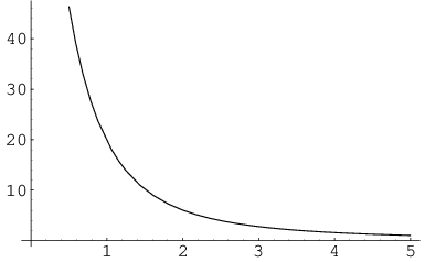
We now show that the conformal factor given by (7.1.1) is such that can be embedded in euclidean :
Lemma 7.3.
Proof.
A general surface of revolution in is described by an embedding (in cartesian coordinates)
where is a standard local coordinate on the circle and we take . Under this map, the euclidean metric of pulls back as
In order for this to be the polar isothermal form (as in equation (32)) of a metric in two dimensions, one must set the coefficient of equal to , yielding
| (43) |
This determines a real function if and only if the condition
| (44) |
is satisfied for all . In our case of interest, we should take
It is easy to check that for all and (44) can be expressed as
which can be verified to hold for . ∎
The embedded surface has cylindrical topology and provides a good picture of the geometry of ; we plot a section of it in Figure 4, using the construction in Lemma 7.3.

It follows from
| (45) |
that this surface is asymptotic to a cylinder of radius for large . Moreover,
implies that it can be completed to a simply-connected surface by adding the single point at . However, this completion fails to be smooth. One way to see this is to consider the scalar curvature of the surface; it depends only on , and can be easily calculated in terms of elliptic integrals from the formula (cf. [27])
We find that this is a positive function on , monotonically decreasing, and with limits
a plot of is shown in Figure 5.

Thus is asymptotically flat for large , which fits with the asymptotics already mentioned. The unboundedness of the curvature as implies that the one-point completion is not smooth at the tip . A rather surprising fact is that this occurs even though the profile curves of the surface approach the symmetry axis at right angles:
| (46) | |||||
(here and are as defined in the proof of Lemma 7.3). Now the limit (45) implies that, as , tangents to the profile curves make an angle of with the direction of the symmetry axis. An elementary result on differential geometry of surfaces of revolution in then allows us to compute the total curvature of from (46) as
This result agrees with what one would obtain for any embedded surface of revolution in asymptotic to a cylinder at one end and smooth at the other end, by the theorem of Gauß–Bonnet.
Any meridian (given by equating to a constant) is a geodesic of the surface . It follows from our proof of Theorem 6.1 that the meridians are incomplete geodesics – any point on them is at finite distance from the tip . This can also be checked from the explicit formulas (32) and (7.1.1). It is also easy to show that the integrand in (43) never vanishes, and this implies that none of the parallels (circles of constant ) is a geodesic (cf. [28], p. 182). More general geodesics on are straightforward to find as an application of Clairaut’s theorem (cf. [28], pp. 183–185).
7.1.2
The metric on the totally geodesic submanifold introduced in Lemma 7.1 can be written as
| (47) |
where
Notice that the prefactor diverges at the points and , where the degree of the maps jump to one. Notice also that depends on both the modulus and the argument of , which makes the computation of the integral in closed form a more difficult task. However, we can calculate some geodesics of even without performing the integral.
Lemma 7.4.
The intervals , , and in the complex plane parametrised by are all geodesics of the metric (47).
Proof.
This follows again from Lemma 4.2. Invariance of the maps
with respect to the isometry defined in (23) imposes the relation
on , this is the equation for the union of the three intervals , and , which are therefore geodesics of . Similarly, considering , invariance under the isometry
leads to the constraint
and this shows that is also a geodesic. ∎
The proof of Theorem 6.1 implies that the geodesic segment in corresponding to , has finite length with respect to the metric (47), and the same is true for any other piece of the intervals in Lemma 7.4 that accumulates at or .
Analogously to the case of above, we can prove that the scalar curvature of becomes unbounded in the neighbourhood of the points where the metric becomes singular:
Lemma 7.5.
The scalar curvature of satisfies
Proof.
We focus on the limit without loss of generality. Consider the paths , with in the unit circle of , given by
These paths parametrise radial segments tending to . (Notice that coincides with defined in the proof of Theorem 6.1 (iii)). An analogous argument to the one in Theorem 6.1, and which we shall not reproduce here, leads to the following estimate for the curvature of each :
Here, is again determined from by (29) and denote positive constants dependent on and on a fixed . Since the right-hand-side is strictly positive when , the scalar curvature must be positive in some neighbourhood of by a continuity argument. The inequality above also implies that the minimal curvature becomes unbounded as , and the result follows. ∎
7.2 Two-lump scattering
Now that we have found some geodesics on , we can interpret them in terms of soliton scattering by plotting the energy density (27) along them.
7.2.1
We have seen that is a surface of revolution. The meridians of this surface define a one-parameter family of geodesics; one of them is
All the other meridians are related to through a fixed target rotation, under which the energy density (27) does not change, and therefore describe the same type of process. This process can be interpreted as a frontal collision of two lumps as we let decrease from a large value to zero; a plot of the energy densities is shown in Figure 6. For large , the configuration can be roughly described as a superposition of two single lumps with symmetry (thus having antipodal endpoints) which are far apart. As decreases, these lumps approach each other (meaning that the regions of large come closer together on the cylinder), and at close distance the approximate symmetry of the energy density breaks down. At this stage, energy density peaks form over antipodal points of a circle transverse to the axis of the cylinder; these peaks become more and more pronounced, with a singularity forming in the limit . As we have seen, this is achieved in finite time, which is a symptom of the incompleteness of the metric. This type of phenomenon is not surprising for the model; it has been reproduced in numerical studies of scattering lumps on the plane [29].


(a) (b) (c) (d)
It is a consequence of Clairaut’s theorem that the geodesics of other than the meridians are complete and do not involve singular peaking. A simple way to understand them (cf. [11, 12]) is to interpret the geodesic flow on as the dynamics of a particle in with position-dependent mass and lagrangian
where
| (48) |
Here, is the (conserved) momentum conjugate to the cyclic coordinate , which can be interpreted as a coupling to the effective potential (48). We plot in Figure 7; it is a monotonically decreasing function and has a horizontal asymptote at as , corresponding to the limit (45). From the plot, it is immediately clear that the complete geodesics of , corresponding to taking , describe reflection collisions. In these processes, the peaking of the energy density as the lumps approach each other is reversed at a certain instant, after which the lump separation grows to infinity. For instance, the sequence (a)(b)(c)(b)(a) of configurations in Figure 6 represents snapshots of one such reflection. Processes of this type are accompanied by a rotation of the overall phase of the field configuration and are generic among the motions on the submanifold .

7.2.2
The geodesics we have found on give three qualitatively distinct two-lump motions:
with
Energy densities of the process described by are plotted in Figure 8. We can say it consists of a frontal collision of two peaked single lumps of the same shape along a longitudinal (straight) line. At collision, the two peaks coalesce and develop a singularity over the midpoint of their initial positions (local maxima of ) in the limit .


(a) (b) (c)
The geodesic describes processes related to the decay of the two-lump (whose energy density exhibits symmetry) to peaked configurations that become singular in the limit . Strictly speaking, this process alone is not of scattering nature because it does not connect configurations of asymptotically well-separated maxima of energy density. Alternatively, one could interpret the geodesic as a tunneling of single-peaked two-lumps through the cylinder, passing through the -symmetric configuration. This is illustrated in Figure 9.


(a) (b) (c) (d) (e)
Finally, the geodesic may be interpreted as a scattering process of two single lumps with the same shape along longitudinal lines positioned antipodally on the cylinder; energy densities are plotted in Figure 10. If the lumps travel past each other, there is again an instant for which the energy density of the configuration has symmetry, and after that each individual lump continues its motion along the longitudinal line with no significant distortion of shape.


(a) (b) (c)
8 Discussion
In this paper, we have considered the adiabatic approximation to the dynamics of solitons in the -model on an infinite cylinder . As in previous studies of this model on other surfaces, for each degree there is a smooth, finite-dimensional moduli space parametrising static solutions (-lumps); in our case, this space is modelled on the space of rational maps and is therefore a complex manifold. We have found that the approximation defines a dynamical system by automorphisms of a natural map specifying the boundary values of the fields. On each fibre, these automorphisms are defined by the geodesic flow of the metric, which is regular and Kähler. By means of this fibration, we avoid making reference to degenerate metrics as in [10]. Although our language could be adapted to deal with lumps on the plane, in that case the boundary values of the fields alone are still not enough to specify a sufficiently fine fibration of the moduli spaces to render the metrics regular.
Lumps of degree one are characterised by a shape function taking values in (the distance of their endpoints), together with a location (a point on if or a transversal circle if ) and a physically irrelevant global phase. Their adiabatic dynamics is trivial: it reduces to uniform motion of their location on the cylinder with shape-independent inertial mass. This is similar to the -model on the plane, where the only possible adiabatic motion of one-lumps is also uniform motion along geodesics, i.e. straight lines [10].
The dynamics of multilumps is more interesting to study. We established that all the metrics for multilumps on the cylinder are incomplete. Again, this parallels an analogous result for lumps on the plane, as put forward by Sadun and Speight in [14]. Incompleteness of the metric translates into the possibility of lump collapse in finite time in the adiabatic approximation. Using standard symmetry considerations, we have found totally geodesic submanifolds for the metrics on two types of fibres , namely for and antipodal, and some geodesics on them. We have also found explicit formulae for the metric on one two-dimensional totally geodesic submanifold of , which involves elliptic integrals. This metric is incomplete, and the corresponding lump collapse can be plotted with no difficulty (Figure 6). Similarly, some of the geodesics we found for and antipodal exhibit lump collapse (Figures 8 and 9). It is still an unsettled question how to interpret finite-time collapse (which is understood as a feature of the adiabatic approximation) at the full field theory level. As the metric becomes singular, one may expect the approximation to break down; on the other hand, numerical simulations of the field theory seem to support the claim that collapse in finite time should also occur in the full dynamics. Another question is whether the dynamics is well defined beyond collapse. A rather striking feature of the geodesics describing collapse that we found is that they all have natural prolongations on the relevant moduli spaces; in particular, for the scattering processes we described on , the whole real -axis can be interpreted as a process of double scattering at of two one-lumps approaching first along a generatrix of the cylinder, then travelling along a transversal circle, and finally separating along the opposite generatrix, which is very natural to expect from our intuition on (second-order) soliton dynamics in two dimensions.
The scattering processes corresponding to the geodesics that we found explicitly turn out to be rather unique when compared to previous results on other surfaces, a fact that is due to the different topology of the cylinder. It should be expected that more generic geodesics will give rise to more familiar processes, in particular the frontal scattering at . In fact, we have found curves on the submanifold which are close to geodesics (in the sense that the Christoffel symbols related to transverse motion are small in some region) and that describe processes of this type.
There is some belief that lump configurations at collapse are supressed at the quantum level. Following Gibbons and Manton [7], the quantum-mechanical version of the adiabatic dynamics should be based on a Schrödinger equation on each using the covariant laplacian of the metric, but as a correction one expects an effective potential term given by the scalar curvature of the moduli space [30]. Accordingly, wavefunctions should be given zero boundary values whenever the scalar curvature diverges. In our examples, we found that the scalar curvatures of and blow up as the boundary of the moduli space is approached upon collapse. In [17], Speight also found a divergence of the scalar curvature of the moduli space of one-lumps on preventing collapse, but our results directly refer to the interacting case and therefore give more substantial support to the hope that the degree of lumps should be conserved in the quantum field theory.
Acknowledgements
I would like to thank Klaus Kirsten, Nick Manton, Avijit Mukherjee, Oliver Schnürer and especially Martin Speight for discussions. This work was supported by the Max-Planck-Gesellschaft, Germany.
Appendix A: Proof of Lemma 4.2
Totally geodesic submanifolds can be characterised by the property that (the continuation of) any geodesic of the ambient metric starting tangent to will never leave . Suppose, for a contradiction, that there is a geodesic of such that
| (49) |
and
| (50) |
It follows from (49) that , and as such it can be regarded as an equivalence class of paths through containing paths that lie entirely on . These paths are fixed by , so for all . Now (50) implies that for any there is at least one element such that . Since , is also a solution to the equation of the geodesics for ; it satisfies the Cauchy data
and is distinct from . This contradicts the Picard–Lindelöf theorem ensuring uniqueness of solutions of ODEs. Hence must be a totally geodesic submanifold.
Appendix B: Proof of Lemma 7.2
The fact that in (38) is analytic for positive real values of follows from the (complex) analyticity of the integrand as a function of , the integrability of the integrand as a function of and the Leibniz rule. To compute in closed form, we use an argument based on the idea that can be extended by analytic continuation to a neighbourhood of the set
We start by rewriting
here, the last two integrals must be interpreted as Cauchy principal values, which are easily seen to exist. To evaluate their sum, we first Wick-rotate to , which leads to
Each of the two terms above can be evaluated in closed form using the result (cf. formula I.(5) in [31])
This yields
| (51) |
We have to now undo the Wick rotation in the expression above to obtain the values of we are interested in. This must be done carefully, since the analytic continuation of branches at the singular point and the square root branches at the origin. Recall that can be represented as a hypergeometric series for (cf. (900.00) in [25]):
| (52) |
(Here and .) So the properties of the analytic continuation of can be deduced from those of Gauß’s . Following common practice, we introduce a branch cut on the real axis from to . On , is single-valued, and it commutes with complex conjugation,
| (53) |
because the coefficients of the series in (52) are real. Across the branch cut, there is a nontrivial monodromy that accounts for a discontinuity
| (54) |
where the top/bottom signs correspond to the limits obtained when approaches the cut from above/below. This result can be obtained by relating Kummer’s solutions of hypergeometric differential equations (cf. [32], Chap. 2). By a similar argument (and (53)), one can show that
| (55) |
We now want to Wick-rotate back to in (51); one way to keep track of the branching of the functions involved is to substitute the final by , with small, real and positive, evaluate in terms of continuous quantities and let at the end. It is convenient to consider the cases and separately. In the first case, we find that the argument of the first in (51) after substution, , has positive imaginary part, and according to (54) above we should then evaluate
On the other hand, the second term in (51) is free from branching, and we can evaluate using (53) and (55)
In the case , the argument of the first in (51) does not lie on the branch cut after rotation, but the square root itself branches on the negative real half-axis, meaning that we should take
(where of course always denotes the principal branch of the square root); we then find using (55)
However, this time the second does branch; since has negative imaginary part, we should take the lower sign in (54) and find
Adding the two terms in each of the two cases and , we finally obtain the result (39).
References
- [1] N.S. Manton: A remark on the scattering of BPS monopoles. Phys. Lett. B 110 (1982) 54–56.
- [2] T.M. Samols: Vortex scattering. Commun. Math. Phys. 145 (1992) 149–180.
- [3] D. Stuart: Dynamics of Abelian Higgs vortices in the near Bogomolny regime. Commun. Math. Phys. 159 (1994) 51–91.
- [4] M.F. Atiyah and N.J. Hitchin: The Geometry and Dynamics of Magnetic Monopoles. Princeton University Press, 1988.
- [5] D.M.A. Stuart: The geodesic approximation for the Yang–Mills–Higgs equations. Commun. Math. Phys. 166 (1994) 149–190.
- [6] M. Namba: Families of Meromorphic Functions on Compact Riemann Surfaces (Lecture Notes in Mathematics 767). Springer-Verlag, 1979.
- [7] G.W. Gibbons and N.S. Manton: Classical and quantum dynamics of BPS monopoles. Nucl. Phys. B 274 (1986) 183–224.
- [8] B.J. Schroers: Quantum scattering of BPS monopoles at low energy. Nucl. Phys. B 367 (1991) 177–214.
- [9] N.M. Romão: Quantum Chern–Simons vortices on a sphere. J. Math. Phys. 42 (2001) 3445–3469, hep-th/0010277.
- [10] R.S. Ward: Slowly-moving lumps in the model in (2+1) dimensions. Phys. Lett. B 158 (1985) 424–428.
- [11] J.M. Speight: Low-energy dynamics of a lump on the sphere. J. Math. Phys. 36 (1995) 796–813, hep-th/9712089.
- [12] J.M. Speight: Lump dynamics in the model on the torus. Commun. Math. Phys. 194 (1998) 513–539, hep-th/9707101.
- [13] J.M. Speight and I.A.B. Strachan: Gravity thaws the frozen moduli of the lump. Phys. Lett. B 457 (1999) 17–22, hep-th/9903264.
- [14] L.A. Sadun and J.M. Speight: Geodesic incompleteness in the model on a compact Riemann surface. Lett. Math. Phys. 43 (1998) 329–334, hep-th/9707169.
- [15] A.M. Din and W.J. Zakrzewski: Skyrmion dynamics in 2+1 dimensions. Nucl. Phys. B 259 (1985) 667–676.
- [16] P.J. Ruback: Sigma model solitons and their moduli space metrics. Commun. Math. Phys. 116 (1988) 645–658.
- [17] J.M. Speight: The geometry of spaces of harmonic maps and ,. J. Geom. Phys. 47 (2003) 343–368, math.DG/0102038.
- [18] M. Haskins and J.M. Speight: The geodesic approximation for lump dynamics and coercivity of the Hessian for harmonic maps. J. Math. Phys. 44 (2003) 3470–3494, hep-th/0301148.
- [19] A.A. Belavin and A.M. Polyakov: Metastable states of two-dimensional isotropic ferromagnets. JETP Lett. 22 (1975) 245–247.
- [20] A. Lichnerowicz: Applications harmoniques et variétés kähleriennes. Symp. Math. Bologna 3 (1970) 341–402.
- [21] R. Remmert: Funktionentheorie 2. Springer-Verlag, 2nd edition, 1995.
- [22] S. Lang: Real and Functional Analysis. Springer-Verlag, 3rd edition, 1993.
- [23] M.P. do Carmo: Riemannian Geometry. Birkhäuser, 1992.
- [24] P.M. Sutcliffe: BPS monopoles. Int. J. Mod. Phys. A 12 (1997) 4663–4705, hep-th/9707009.
- [25] P.F. Byrd and M.D. Friedman: Handbook of Elliptic Integrals for Engineers and Physicists. Springer-Verlag, 1954.
- [26] F. Tricomi: Elliptische Funktionen. Akademische Verlagsgesellschaft Geest & Portig, Leipzig, 1948.
- [27] J. Jost: Differentialgeometrie und Minimalflächen. Springer-Verlag, 1994.
- [28] A. Pressley: Elementary differential geometry. Springer-Verlag, 2001.
- [29] R.A. Leese: Low-energy scattering of solitions in the model. Nucl. Phys. B 344 (1990) 33–72.
- [30] I.G. Moss and N. Shiiki: Quantum mechanics on moduli spaces. Nucl. Phys. B 565 (2000) 345–362, hep-th/9904023.
- [31] M.L. Glasser: Definite integrals of the complete elliptic integral . J. Res. Nat. Bur. Standards Sect. B 80B (1976) 313–323.
- [32] K. Iwasaki, H. Kimura, S. Shimomura and Y. Masaaki: From Gauss to Painlevé. Vieweg, 1991.