Eigenvalues of Hermite and Laguerre ensembles: Large Beta Asymptotics

This paper provides insight into the shape of random matrix laws such as the finite semi-circle law, the finite quarter-circle law and its generalization. We begin with a simple example. Suppose $A$ is a random $k\times k$ complex matrix with real and imaginary parts all i.i.d. standard normals. Let $S=(A+A^{H})/2$ be the Hermitian part of $A$. The matrix $S$ has a distribution commonly known as the Gaussian Unitary Ensemble; this matrix distribution and the joint distribution of its (real) eigenvalues have been well studied. For a good reference on the subject, see Mehta [10].

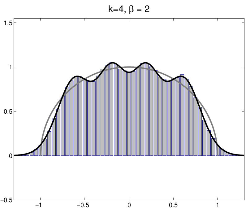
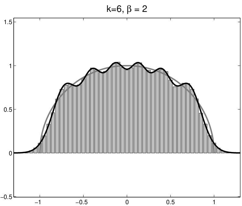
We draw below histograms of normalized eigenvalues taken from this distribution, the known theoretical distribution (see [10, page 93]), and the semicircle limit corresponding to $k\rightarrow\infty$. For the histograms, we have chosen $40,000$ samples from the GUE with $k=4$ and $k=6$.

Notice, for $k$ finite, the $k$ “bumps” in the distribution that wiggle above and below the semi-circle. A natural question to many engineers, physicists, mathematicians, and other scientists who have seen these pictures is whether they can be well approximated by the sum of $k$ appropriately chosen Gaussians. (Of course when $k=1$, this is exactly true.) The answer, as proved in this paper, is yes. We give a sum of Gaussians approximation that is asymptotically correct for the $\beta\rightarrow\infty$ limit but useful even for small values of $\beta$.

For those well versed in random matrix theory, the GUE is the $\beta=2$ case of a Hermite matrix ensemble [10]. Had we started with $A$ real (quaternion), we would have the Gaussian Orthogonal (Symplectic) Ensemble corresponding to $\beta=1$ ($\beta=4$).

The joint eigenvalue density $f_{\beta}^{H}(\lambda_{1},\ldots,\lambda_{k})$ defined on $\mathbb{R}^{k}$ for the $k$ eigenvalues for an arbitrary $\beta>0$ is given in the formula below.

Note the “repulsion” factor $\Delta(\Lambda)\equiv\Delta(\lambda_{1},\ldots,\lambda_{k})\equiv\prod\limits_{1\leq i<j\leq k}|\lambda_{i}-\lambda_{j}|$.

Similarly, for the $k\times k$ Laguerre ensembles of statistics (Wishart matrix theory), the joint eigenvalues density $F_{\beta,a}^{L}$ is defined on $[0,\infty)^{k}$ for arbitrary $\beta$ and parameter $a>(k-1)\beta/2$, and is given below; once again note the repulsion factor $\Delta(\Lambda)$:

where

In [5], we have found (real) tridiagonal matrix models whose eigenvalue distributions are given by (1) and (2); we depict the distributions in Table 1. Note that the variables have either standard normal distribution or a $\chi$ distribution (sometimes scaled by $\sqrt{2}$).

For generating efficiently eigenvalues for the $\beta$-ensemble distributions, we recommend using the tridiagonal/bidiagonal model above.

The marginal density of a single eigenvalue (known as the level density) can be computed in the case of the Hermite ensembles for $\beta$ an even integer [2] using the MOPS software [6]. For general $\beta$ perhaps a little more research is needed, but it is likely that computational techniques are not far out of reach.

For fixed $k$ and general $\beta$ one finds that for $\beta$ getting larger, the bumps of Figure 1 get “bumpier”. To be precise, for the Hermite ensembles, we prove here that at $\beta=\infty$ the bumps become delta functions at the roots of the $k$th Hermite polynomial, while for $\beta$ large, the bumps behave like Gaussians centered at these roots with variance $O(1/\beta)$.

The model of $\beta$ as an inverse temperature is apparent from (1). As $\beta$ goes to $0$, the strength of the repulsion factor $\Delta(\Lambda)$ decreases until annihilation; the interdependence among eigenvalues disappears, and the randomness increases (each eigenvalue behaves like an independent Gaussian). In the frozen state ($\beta=\infty$), we can imagine the $k$ eigenvalues fixed at the roots of the Hermite polynomial. Warming the system a little ($\beta$ very large but not infinite) gives the particles a little energy, and the eigenvalues have Gaussian distribution to first order around the Hermite polynomial roots.

Similarly, in the Laguerre case, at $\beta=0$, the eigenvalues become i.i.d. variables with distribution $\chi_{2a}^{2}$. As $\beta$ grows the eigenvalues have Gaussian distribution to first order around the Laguerre polynomial roots, while at $\beta=\infty$ we reach the freezing point when the eigenvalues are fixed at those roots.

In the following, we use first order eigenvalue perturbation theory and the tridiagonal ensembles in [5] to rigorously investigate this phenomenon mathematically obtaining precisely the asymptotic variance along with the mean.

These results draw a parallel to the Tracy-Widom laws [13, 14] for the $\beta=1,2,4$-Hermite ensembles, later extended to $\beta=1,2$-Laguerre ensembles by Johansson [8] and Johnstone [9].

The Tracy-Widom laws compute the fluctuation in the distribution of the largest eigenvalue of a $\beta$-Hermite ensemble with $\beta=1,2,4$, as $k\rightarrow\infty$, and obtain it in terms of the solution to a Painleve differential equation. From the semicircle law, we know that as $n\rightarrow\infty$, regardless of $\beta$, the largest eigenvalue (scaled by $\sqrt{2k\beta}$) goes to $1$. From Theorem 3.1, constrained to $i=1$, with the help of [11] and [1, page 450], we obtain Corollary 3.3, which gives an intuition of how the $\beta=1,2,4$ Tracy-Widom distributions evolve towards a normal distribution at $\beta=\infty$.

The theoretical results of Section 5 are similar to the “Central Limit Theorems”, i.e. the computation of the global fluctuations from the semicircle and semicircle-type laws done by Johansson in [7] for Hermite-like ensembles of any $\beta$ and by Silverstein and Bai [12] for a class of Laguerre-like ensembles with real or complex entries ($\beta=1,2$). Roughly said, the eigenvalues can be thought of as fluctuating (like Gaussians) around the roots of the corresponding orthogonal polynomial as $\beta$ grows large; if one lets $n$ grow large, too, the global eigenvalue fluctuation becomes a Gaussian process. The larger $1/\beta$, the “warmer” it gets, and the larger the “vibration”. The larger $\beta$, the “cooler” it gets, and the eigenvalues “freeze” into place.

At the end of Section 5 we perform computational experiments to see how good the $\beta$ large approximation is even for relatively small $k$ and $\beta$.

In this section we present two lemmas we need in the proofs of our main results (Theorems 3.1 and 4.1).

The first lemma involves perturbation theory; for a good reference on Perturbation theory and a more general form of the result below, see Demmel’s book [3, Section 4.3].

The second result is an approximation lemma for the $\chi_{r}$ distribution as $r$ grows large.

Let $k$ be fixed, and let $h_{1}^{(k)},\ldots,h_{k}^{(k)}$ be the roots of the $k$th univariate Hermite polynomial $H_{k}$ (where the Hermite polynomials $H_{0}(x),H_{1}(x),\ldots$ are orthonormal with respect to the weight $e^{-x^{2}}$ on $(-\infty,\infty)$).

Let $A_{\beta}$ be a random matrix from the $\beta$-Hermite ensemble of size $k$, scaled by $1/\sqrt{2k\beta}$. For the remainder of this section, we think of $\beta$ as a parameter.

We state and prove the following theorem.

Letting $k\rightarrow\infty$ in Theorem 3.1, we obtain the Corollary below.

Let $k$ be fixed. Given a fixed $\gamma>0$, let $l_{1}^{(k)},\ldots,l_{k}^{(k)}$ be the roots of the $k$th Laguerre polynomial of parameter $\gamma-1$, $L^{\gamma-1}_{k}$. Note that for any $\gamma\geq 0$, the Laguerre polynomials $L_{0}^{\gamma},L_{1}^{\gamma},\ldots$ are orthonormal with respect to the weight $x^{\gamma}e^{-x}$ on $[0,\infty)$; for $\gamma\in[-1,0)$ they admit formal definitions.

Let $B_{\beta}$ be a random matrix from the $\beta$-Laguerre ensemble of size $k$ and parameter $a_{\beta}$, scaled by $1/k\beta$. For the remainder of this section, we think of $\beta$ as a parameter. Suppose that, as $\beta$ grows large,

Note that the requirement $a_{\beta}\!>\!(k-1)\beta/2$ constrains $\gamma$ to be positive.

We can compare the large $\beta$ asymptotics to the theoretical answer for the distribution of a randomly chosen eigenvalue. For large $n$, this is the well-know semicircle law (for the Hermite ensembles) or equivalent thereof (for Laguerre ensembles), but we are interested in finite $n$.

We found that even for $\beta$ small, the approximation can be quite reasonable.

We summarize the large $\beta$ answer as a sum of Gaussians in Corollaries 5.1 and 5.2.

While these approximations are simple enough (a sum of Gaussians is an easily recognizable shape that is also easy to work with), one may wonder how big $\beta$ has to be in order for these approximations to become “accurate” (for example, in order to appear accurate in a plot, the approximations have to be accurate to about 2-3 digits). We have found that, in either of the two cases, the answer is surprisingly low.

In the following two subsections, we have used only even integer values of $\beta$ for our plots, because (in addition to $\beta=1$) those are the only ones for which (to the best of our knowledge) there are exact formulas for the level densities. The plots were obtained with the help of our Maple Library, MOPs (Multivariate Orthogonal Polynomials (symbolically)), which was used for computing the orthogonal and Jack polynomial quantities involved; these were translated into polynomials which were then plotted in MATLAB. For a reference on MOPs see [6].

References

• [1] M. Abramowitz and I.A. Stegun, editors. Handbook of Mathematical Functions. Dover Publications, New York, 1970.
• [2] T. Baker and Peter Forrester. The Calogero-Sutherland model and generalized classical polynomials. Commun.Math.Phys., 188:175–216, 1997.
• [3] James Demmel. Applied Numerical Linear Algebra. SIAM, Philadelphia, 1997.
• [4] Persi Diaconis. Patterns in eigenvalues: the 70th Josiah Willard Gibbs Lecture. Bulletin of the American Mathematical Society, 40:155–178, 2003.
• [5] Ioana Dumitriu and Alan Edelman. Matrix models for beta-ensembles. J. Math. Phys., 43:5830–5847, 2002.
• [6] Ioana Dumitriu, Alan Edelman, and Gene Shuman. MOPS: Multivariate Orthogonal Polynomials (symbolically). 2004. Preprint.
• [7] Kurt Johansson. On fluctuations of random hermitian matrices. Duke Math. J., 91:151–203, 1998.
• [8] Kurt Johansson. Shape fluctuations and random matrices. Commun. Math. Phys., 209:437–476, 2000.
• [9] Iain M. Johnstone. On the distribution of the largest principal component. Ann. of Stat., 29(2):295–327, 2001.
• [10] Madan Lal Mehta. Random Matrices. Academic Press, Boston, second edition, 1991.
• [11] Gábor Szegö. Orthogonal Polynomials. American Mathematical Society, Providence, 1975. 4th edition.
• [12] Jack W. Silverstein and Z.D. Bai. CLT of linear spectral statistics of large dimensional sample covariance matrices. preprint, 2003. Accepted for publication in Annals. of Probab.
• [13] Craig A. Tracy and Harold Widom. On orthogonal and symplectic matrix ensembles. J. Stat. Phys., 92:809–835, 1996.
• [14] Craig A. Tracy and Harold Widom. The distribution of the largest eigenvalue in the Gaussian ensembles. In Calogero-Moser-Sutherland Models, CRM Series in Mathematical Physics, volume 4, pages 461–472. Springer-Verlag, 2000.