A Guide to Stochastic Löwner Evolution and its Applications

Wouter Kager Bernard Nienhuis Affiliation: Affiliation: Institute for Theoretical Physics Affiliation: University of Amsterdam Affiliation: Valckenierstraat 65 Affiliation: 1018 XE Amsterdam, the Netherlands Affiliation: e-mail: kager@science.uva.nl and nienhuis@science.uva.nl

Abstract

This article is meant to serve as a guide to recent developments in the study of the scaling limit of critical models. These new developments were made possible through the definition of the Stochastic Löwner Evolution (SLE) by Oded Schramm. This article opens with a discussion of Löwner’s method, explaining how this method can be used to describe families of random curves. Then we define SLE and discuss some of its properties. We also explain how the connection can be made between SLE and the discrete models whose scaling limits it describes, or is believed to describe. Finally, we have included a discussion of results that were obtained from SLE computations. Some explicit proofs are presented as typical examples of such computations. To understand SLE sufficient knowledge of conformal mapping theory and stochastic calculus is required. This material is covered in the appendices.

Key words:

scaling limits, critical exponents, conformal invariance, conformal mappings, stochastic processes, Löwner’s equation.

1 Introduction

The Stochastic Löwner Evolution appears as a new branch to an already varied palette of techniques available for the study of continuous phase transitions in two dimensions. Phase transitions are among the most striking phenomena in physics. A small change in an environmental parameter, such as the temperature or the external magnetic field, can induce huge changes in the macroscopic properties of a system. Typical examples are liquid-gas transitions and spontaneous magnetization in ferromagnets. Many more examples are observed in nature in the most diverse systems, and for a long time physicist have been searching for explanations of these phenomena (for a nice introduction explaining the notions involved in the physical interpretation of these phenomena, see for example [49]).

To characterize phase transitions, one introduces an order parameter, a quantity which vanishes on one side of the phase transition and is non-zero on the other side. For magnets one uses the magnetization, while for liquid-gas transitions the density difference between the two phases defines the order parameter. At the phase transition, the change in the order parameter can be either discontinuous or continuous. In the former case the transition is called first-order, in the latter case it is called continuous or second-order.

It is found experimentally that near continuous phase transitions many observable quantities have a power-law dependence on their parameters with non-integer powers, called critical exponents. Thus, the order parameter for example typically behaves like $(T_{c}-T)^{\beta}$ just below the transition temperature $T_{c}$ , and observables such as the specific heat or the susceptibility diverge as $|T-T_{c}|^{-\alpha}$ near $T_{c}$ . Moreover, the critical exponents appear to be universal in the sense that there are classes of different systems, that show critical behaviour with the exact same values of the critical exponents. This phenomenon is known as universality (some examples are given in the standard reference [44] on the theory of critical phenomena).

Universality allows one to draw parallels between different systems and different types of phase transitions. Theoretically, it leads to the conclusion that the behaviour near a critical point can be described by just a few relevant parameters, and that many microscopic details of the system become irrelevant near the critical point. It turns out that the critical exponents are largely determined by just the dimension of the system, and the dimension and symmetries of the order parameter. This justifies the use of simple model systems, in which all the details of the interactions have been neglected, to investigate critical behaviour. Examples of such models are the Ising model, the $q$ -state Potts models and O( $n$ ) models. The concept of universality is particularly useful in those cases where one of these simple models can be solved exactly, because such solutions determine the universal properties of a whole class of systems, including those far too difficult to solve exactly.

The behaviour of a system near a transition point is governed by the fluctuations in the system. When one approaches the critical point from the disordered phase, these local fluctuations tend to be correlated over larger and larger distances as one gets closer to the transition point. The typical length-scale $\xi$ of these correlations, the correlation length, diverges as one approaches the critical point. This led physicists to introduce the idea of length-rescaling [26] as a tool for studying critical phenomena, and ultimately led to the formulation of the renormalization group approach [61]. The idea of this approach is that if we look at the system at successively larger scales, the correlation length will be successively reduced. Away from the critical point the correlation length is finite, and rescaling drives us further away from the transition, but at the critical point the correlation length is infinite, and the system is invariant under rescaling.

The hypothesis of scale-invariance led to the development of several techniques for the computation of critical exponents and other observables of critical behaviour, such as correlation functions. One of these techniques is the successful Coulomb Gas method [46], which produces exact results provided certain qualitative assumptions are valid.

Another development came from the idea that we need not restrict ourselves to studying scale-invariance for a system as a whole, but that we might consider scaling properties locally. More precisely, the system can be rescaled with a factor that depends on the position, and we may wonder if the system is invariant under such transformations. This approach led people to believe that in the continuum limit, many model systems are not just scale-invariant, but are in fact conformally invariant [14]. The natural realm for studying conformally invariant behaviour is that of two-dimensional systems, since in two dimensions the group of conformal transformations is so much richer than in higher dimensions. Over the years, the assumption of conformal invariance has indeed been successful in explaining critical behaviour in two-dimensional systems. The assumption is supported by the agreement of the results with the results from exactly solvable models [8].

Many questions remain, especially from the mathematical point of view. The physicist intuitively believes that there exists a continuum or scaling limit of his discrete models when the lattice spacing goes to zero. But when exactly does this limit exist? What does the limit model look like? Is it indeed conformally invariant? Such questions have puzzled both mathematicians and physicists for a long time, and answers to these questions have seemed quite far away.

A big step forward was made when Oded Schramm [53] combined an old idea of Karl Löwner [43] (who later changed his name to Charles Loewner) from univalent-function theory with stochastic calculus. This led to the definition of the one-parameter family of Stochastic Löwner Evolutions, $\mbox{SLE}_{\kappa}$ (see [58] for a mathematical review). Schramm proved that if the loop-erased random walk has a scaling limit, and if this limit is conformally invariant, then it must be described by $\mbox{SLE}_{2}$ . He made similar conjectures relating critical percolation to $\mbox{SLE}_{6}$ and uniform spanning trees to $\mbox{SLE}_{8}$ .

Schramm’s conjectures for loop-erased random walks and uniform spanning trees were later proved by Lawler, Schramm and Werner [40] using SLE techniques. Independently, and using different methods, Smirnov [56] proved the existence and conformal invariance of the scaling limit of critical site percolation on the triangular lattice, thus establishing the connection with $\mbox{SLE}_{6}$ . It is believed that many other models in two dimensions, such as the self-avoiding walk, the $q$ -state Potts models and the O( $n$ ) models also have a conformally invariant scaling limit that is described by an $\mbox{SLE}_{\kappa}$ for some characteristic value of $\kappa$ .

The goal of the present article is to explain Schramm’s idea to an audience of both physicists and mathematicians. We place emphasis on how the connection between the discrete models and SLE is made, and we have included several typical SLE computations to explain how results can be derived from SLE. The article is organized as follows. Section 2 contains a few preliminaries that are required to follow the main line of thought. In section 3 we introduce Löwner evolutions, and define SLE. The section includes a discussion of the Löwner equation in a deterministic setting as an aid to the reader in understanding the relation between SLE and random paths.

Section 4 then gives an overview of the main properties of SLE and the random SLE paths. The connection between SLE and discrete models is discussed in section 5. We give explicit descriptions of those models that are known rigorously to converge to SLE, and we also consider the conjectured connections between SLE and self-avoiding walks, Potts models and O( $n$ ) models. Examples of results obtained from SLE are given in section 6. We have included several worked-out proofs in the text, explaining how things can be calculated from SLE. The article ends with a short discussion.

To make the article self-contained, the appendices deal with the background material that is needed to fully understand all the details of the main text. In addition, we have intended these appendices to make the mathematical literature on SLE more accessible to interested readers, who may not have all the required background knowledge. For this reason, the appendices cover more material than is strictly required for the present article. Appendix A deals with conformal mapping theory. We present some general results of the theory, and focus on topics that are specific for SLE. Appendix B is about stochastic processes, and includes an introduction to the measure-theoretic background of probability theory.

2 Preliminaries

In this short section we give a quick overview of notations and some basic results concerning conformal mapping theory that are used throughout this article. For a more comprehensive treatment of this material including illustrations we refer to appendix A.

First, some notation. We shall write $\mathbbm{C}$ for the complex plane, and $\mathbbm{R}$ for the set of real numbers. The open upper half-plane $\{z:\mathop{\rm Im\,}\nolimits z>0\}$ is denoted by $\mathbbm{H}$ , and the open unit disk $\{z:|z|<1\}$ by $\mathbbm{D}$ . We shall only consider domains whose boundary is a continuous curve, and this implies that the conformal maps we work with have well-defined limit values on the boundary.

Now suppose that $D$ is a simply connected domain with continuous boundary, and that $z_{1}$ , $z_{2}$ , $z_{3}$ and $z_{4}$ are distinct points on $\partial D$ , ordered in the counter-clockwise direction. Then we can map $D$ onto a rectangle $(0,L)\times(0,{\rm i}\pi)$ in such a way that the arc $[z_{1},z_{2}]$ of $\partial D$ maps onto $[0,{\rm i}\pi]$ , and $[z_{3},z_{4}]$ maps onto $[L,L+{\rm i}\pi]$ . The length $L>0$ of this rectangle is determined uniquely, and is called the $\pi$ -extremal distance between $[z_{1},z_{2}]$ and $[z_{3},z_{4}]$ in $D$ .

A compact subset $K$ of $\overline{\mathbbm{H}}$ such that $\mathbbm{H}\setminus K$ is simply connected and $K=\overline{K\cap\mathbbm{H}}$ is called a hull (it is basically a compact set bordering on the real line). For any hull $K$ there exists a unique conformal map, denoted by $g_{K}$ , which sends $\mathbbm{H}\setminus K$ onto $\mathbbm{H}$ and satisfies the normalization

\lim_{z\mathrel{\rightarrow}\infty}\big(g_{K}(z)-z\big)=0.

(1)

This map has an expansion for $z\mathrel{\rightarrow}\infty$ of the form

g_{K}(z)=z+\frac{a_{1}}{z}+\ldots+\frac{a_{n}}{z^{n}}+\ldots

(2)

where all expansion coefficients are real. The coefficient $a_{1}=a_{1}(K)$ is called the capacity of the hull $K$ .

The capacity of a nonempty hull $K$ is a positive real number, and satisfies a scaling rule and a summation rule. The scaling rule says that if $r>0$ then $a_{1}(rK)=r^{2}a_{1}(K)$ . The summation rule says that if $J\subset K$ are two hulls and $L$ is the closure of $g_{J}(K\setminus J)$ , then $g_{K}=g_{L}\circ g_{J}$ and $a_{1}(K)=a_{1}(J)+a_{1}(L)$ . The capacity of a hull is bounded from above by the square of the radius of the smallest half-disk that contains the hull and has its centre on the real line.

3 Löwner evolutions

This section is devoted to the Löwner equation and its relation to paths in the upper half-plane. In this section, we will first discuss the Löwner equation in a deterministic setting. We will show how one can describe a given continuous path by a family of conformal maps, and we will prove that these maps satisfy Löwner’s differential equation. Then we will prove that conversely, the Löwner equation generates a family of conformal maps, that may of may not describe a continuous curve. Finally, we move on to the definition of the stochastic Löwner evolution. This section is based on ideas from Lawler, Schramm and Werner [35], Lawler [33], and Rohde and Schramm [51].

3.1 Describing a path by the Löwner equation

Suppose that $\gamma(t)$ (where $t\geq 0$ ) is a continuous path in $\overline{\mathbbm{H}}$ which starts from $\gamma(0)\in\mathbbm{R}$ . We allow the path to hit itself or the real line, but if it does, we require the path to reflect off into open space immediately. In other words, the path is not allowed to enter a region which has been disconnected from infinity by $\gamma[0,t]\cup\mathbbm{R}$ . To be specific, let us denote by $H_{t}$ for $t\geq 0$ the unbounded connected component of $\mathbbm{H}\setminus\gamma[0,t]$ , and let $K_{t}$ be the closure of $\mathbbm{H}\setminus H_{t}$ . Then we require that for all $0\leq s<t$ , $K_{s}$ is a proper subset of $K_{t}$ . See figure 1 for a picture of a path satisfying these conditions.

We further impose the conditions that for all $t\geq 0$ the set $K_{t}$ is bounded, so that $\{K_{t}:t\geq 0\}$ is a family of growing hulls, and that the capacity of these hulls eventually goes to infinity, i.e. $\lim_{t\mathrel{\rightarrow}\infty}a_{1}(K_{t})=\infty$ . The latter condition implies that the path eventually has to escape to infinity, but there do exist paths to infinity whose capacities remain finite (a formula for the capacity is given at the end of appendix A.4). Now let us state the purpose of this subsection.

For every $t\geq 0$ we set $g_{t}:=g_{K_{t}}$ , and we further define the real-valued function $U_{t}:=g_{t}(\gamma(t))$ (this is the point to which the tip of the path is mapped). The purpose of this subsection is to prove that the maps $g_{t}$ satisfy a simple differential equation, which is driven by $U_{t}$ . Ideas for the proof were taken from [35]. For a different, probabilistic approach, see [33]. The first thing that we show, is that we can choose the time parameterization of $\gamma$ such that the capacity grows linearly in time. Clearly, this fact is a direct consequence of the following theorem.

Theorem 3.1

Both $a_{1}(K_{t})$ and $U_{t}$ are continuous in $t$ .

Proof.

The proof relies heavily on properties of $\pi$ -extremal distance, and we refer to the chapter on extremal length, sections 4.1–4.5 and 4.11–4.13, in Ahlfors [2] for the details. We shall prove left-continuity first.

Without loss of generality we may assume that $\gamma(0)=0$ . Fix $t>0$ , let $R$ be a large number, say at least several times the radius of $K_{t}$ , and let $C_{R}$ be the upper half of the circle with radius $2R$ centred at the origin. Fix $\varepsilon>0$ . Then by continuity of $\gamma(t)$ , there exists a $\delta>0$ such that $|\gamma(t)-\gamma(u)|<\varepsilon/2$ for all $u\in(t-\delta,t)$ . Now let $C_{\varepsilon}$ be the circle with radius $\varepsilon$ and centre $\gamma(t)$ , and let $S$ be the arc of this circle in the domain $H_{t}$ . Then this set $S$ disconnects $K_{t}\setminus K_{t-\delta}$ from infinity in $H_{t-\delta}$ , see figure 1. Observe that the set $K_{t}\setminus K_{t-\delta}$ may be just a piece of $\gamma$ , but that it can also be much larger, as in the figure.

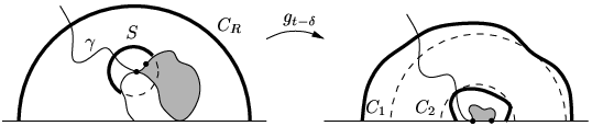
Refer to caption — Figure 1: A path $\gamma$ . The two points represent $\gamma(t)$ and $\gamma(t-\delta)$ , and the shaded area is the set $K_{t}\setminus K_{t-\delta}$ . For clarity, the arc $C_{R}$ is drawn much smaller than it is in the proof.

For convenience let us denote by $\Omega$ the part of the domain $H_{t-\delta}$ that lies below $C_{R}$ . Let $\mathcal{L}$ be the $\pi$ -extremal distance between $S$ and $C_{R}$ in $\Omega$ . By the properties of $\pi$ -extremal distance, because the circle with radius $R$ and centre at $\gamma(t)$ lies below $C_{R}$ , $\mathcal{L}$ must be at least $\log(R/\varepsilon)/2$ . Note that since $\pi$ -extremal distance is invariant under conformal maps, $\mathcal{L}$ is also the $\pi$ -extremal distance between $g_{t-\delta}(C_{R})$ and $g_{t-\delta}(S)$ in $g_{t-\delta}(\Omega)$ . This allows us to find an upper bound on $\mathcal{L}$ .

To get this upper bound, we draw two concentric semi-circles $C_{1}$ and $C_{2}$ , the first hitting $g_{t-\delta}(C_{R})$ on the inside, and the second hitting $g_{t-\delta}(S)$ on the outside as in figure 1 (this is always possible if $R$ was chosen large enough). Note that by the hydrodynamic normalization of the map $g_{t-\delta}$ , we have an upper bound on the radius of $C_{1}$ , which depends only on $R$ (this follows for example from theorem A.11). As is explained in Ahlfors, this means that the $\pi$ -extremal distance $\mathcal{L}$ satisfies an inequality of the form $\mathcal{L}\leq\log(C(R)/r)$ , where $C(R)$ depends only on our choice of $R$ , and $r$ is the radius of the inner half-circle $C_{2}$ . But $\mathcal{L}$ was at least $\log(R/\varepsilon)/2$ , implying that $r$ can be made arbitrarily small by choosing $\delta$ small enough. It follows that for every $\varepsilon>0$ there exists a $\delta>0$ such that the set $K_{t,\delta}:=g_{t-\delta}(K_{t}\setminus K_{t-\delta})$ is contained in a half-disk of radius $\varepsilon$ . But then by the summation rule of capacity $a_{1}(K_{t})-a_{1}(K_{t-\delta})=a_{1}(K_{t,\delta})\leq\varepsilon^{2}$ , proving left-continuity of $a_{1}(K_{t})$ .

To prove left-continuity of $U_{t}$ , let $\delta$ and $\varepsilon$ be as above, and denote by $g_{t,\delta}$ the normalized map $g_{K_{t,\delta}}$ associated with the hull $K_{t,\delta}$ . It is clearly sufficient to show that $g_{t,\delta}$ converges uniformly to the identity as $\delta\mathrel{\downarrow}0$ (remember that $U_{t}$ is defined as $g_{t}(\gamma(t))$ and refer to figure 1). To prove this, we may assume without loss of generality that the set $K_{t,\delta}$ is contained within the disk of radius $\varepsilon$ centred at the origin, since the claim remains valid under translations over the real line. But then theorem A.11 says that if $|z|\geq 2\varepsilon$ , then

|g_{t,\delta}(z)-z|\leq\sum_{n=1}^{\infty}\frac{a_{n}(K_{t,\delta})}{|z|^{n}}\leq\varepsilon\sum_{n=1}^{\infty}\frac{\varepsilon^{n}}{(2\varepsilon)^{n}}=\varepsilon.

(3)

This shows that the map $g_{t,\delta}$ converges uniformly to the identity. Left-continuity of $U_{t}$ follows. In the same way we can prove right-continuity of $a_{1}(K_{t})$ and $U_{t}$ . ∎

Theorem 3.2

Let $\gamma(t)$ be parameterized such that $a_{1}(K_{t})=2t$ . Then for all $z\in\mathbbm{H}$ , as long as $z$ is not an element of the growing hull, $g_{t}(z)$ satisfies the Löwner differential equation

\frac{\partial}{\partial{t}}g_{t}(z)=\frac{2}{g_{t}(z)-U_{t}},\quad g_{0}(z)=z.

(4)

Proof.

Our proof is based on the proof of theorem 3.1 and the Poisson integral formula, which states that the map $g_{t,\delta}$ satisfies

g_{t,\delta}(z)-z=\frac{1}{\pi}\int_{-\infty}^{\infty}\frac{\mathop{\rm Im\,}\nolimits g_{t,\delta}^{-1}(\xi)}{g_{t,\delta}(z)-\xi}\,{\rm d}{\xi},\qquad z\in\mathbbm{H}\setminus K_{t,\delta}

(5)

while the capacity $a_{1}(K_{t,\delta})$ is given by the integral

a_{1}(K_{t,\delta})=\frac{1}{\pi}\int_{-\infty}^{\infty}\mathop{\rm Im\,}\nolimits g_{t,\delta}^{-1}(\xi)\,{\rm d}{\xi}.

(6)

See appendix A.4 for more information.

First consider the left-derivative of $g_{t}(z)$ . Using the same notations as in the proof of theorem 3.1 we can write $g_{t}=g_{t,\delta}\circ g_{t-\delta}$ . We know that $g_{t,\delta}$ converges to the identity as $\delta\mathrel{\downarrow}0$ , and that the support of $\mathop{\rm Im\,}\nolimits g_{t,\delta}^{-1}$ shrinks to the point $U_{t}$ . Moreover, using the summation rule of capacity and our choice of time parameterization, equation (6) gives $\int\mathop{\rm Im\,}\nolimits g_{t,\delta}^{-1}(\xi)\,{\rm d}{\xi}=2\pi\delta$ . Hence from equation (5) we get

\lim_{\delta\mathrel{\downarrow}0}\frac{g_{t}(z)-g_{t-\delta}(z)}{\delta}=\lim_{\delta\mathrel{\downarrow}0}\frac{1}{\pi\delta}\int\frac{\mathop{\rm Im\,}\nolimits g_{t,\delta}^{-1}(\xi)}{g_{t,\delta}\big(g_{t-\delta}(z)\big)-\xi}\,{\rm d}{\xi}=\frac{2}{g_{t}(z)-U_{t}}.

(7)

In the same way one obtains the right-derivative. ∎

3.2 The solution of the Löwner equation

In the previous subsection, we started from a continuous path $\gamma$ in the upper half-plane. We proved that the corresponding conformal maps satisfy the Löwner equation, driven by a suitably defined continuous function $U_{t}$ . In this subsection, we will try to go the other way around. Starting from a driving function $U_{t}$ , we will prove that the Löwner equation generates a (continuous) family of conformal maps $g_{t}$ onto $\mathbbm{H}$ . The proof follows Lawler [33].

So suppose that we have a continuous real-valued function $U_{t}$ . Consider for some point $z\in\overline{\mathbbm{H}}\setminus\{0\}$ the Löwner differential equation

\frac{\partial}{\partial{t}}g_{t}(z)=\frac{2}{g_{t}(z)-U_{t}},\qquad g_{0}(z)=z.

(8)

This equation gives us some immediate information on the behaviour of $g_{t}(z)$ . For instance, taking the imaginary part we obtain

\frac{\partial}{\partial{t}}\mathop{\rm Im\,}\nolimits g_{t}(z)=\frac{-2\,\mathop{\rm Im\,}\nolimits g_{t}(z)}{(\mathop{\rm Re\,}\nolimits g_{t}(z)-U_{t})^{2}+(\mathop{\rm Im\,}\nolimits g_{t}(z))^{2}}.

(9)

This shows that for fixed $z\in\mathbbm{H}$ , $\partial_{t}\mathop{\rm Im\,}\nolimits[g_{t}(z)]<0$ , and hence that $g_{t}(z)$ moves towards the real axis. Further, points on the real axis will stay on the real axis.

For a given point $z\in\overline{\mathbbm{H}}\setminus\{0\}$ , the solution of the Löwner equation is well-defined as long as $g_{t}(z)-U_{t}$ stays away from zero. This suggests that we define a time $\tau(z)$ as the first time $\tau$ such that $\lim_{t\uparrow\tau}(g_{t}(z)-U_{t})=0$ , setting $\tau(z)=\infty$ if this never happens. Note that as long as $g_{t}(z)-U_{t}$ is bounded away from zero, equation (9) shows that the time derivative of $\mathop{\rm Im\,}\nolimits[g_{t}(z)]$ is bounded in absolute value by some constant times $\mathop{\rm Im\,}\nolimits[g_{t}(z)]$ . For points $z\in\mathbbm{H}$ this shows that in fact, $\tau(z)$ must be the first time when $g_{t}(z)$ hits the real axis. We set

H_{t}:=\{z\in\mathbbm{H}:\tau(z)>t\},\qquad K_{t}:=\{z\in\overline{\mathbbm{H}}:\tau(z)\leq t\}.

(10)

Then $H_{t}$ is the set of points in the upper half-plane for which $g_{t}(z)$ is still well-defined, and $K_{t}$ is the closure of its complement, i.e. it is the hull which is excluded from $H_{t}$ . Our goal is now to prove the following theorem.

Theorem 3.3

Let $U_{t}$ be a continuous real-valued function, and for every $t\geq 0$ let $g_{t}(z)$ be the solution of the Löwner equation (8). Define the set $H_{t}$ as in (10). Then $g_{t}(z)$ is a conformal map of the domain $H_{t}$ onto $\mathbbm{H}$ which satisfies

g_{t}(z)=z+\frac{2t}{z}+O\left(z^{-2}\right),\qquad z\rightarrow\infty.

(11)

Proof.

It is easy to see from (8) that $g_{t}$ is analytic on $H_{t}$ . We will prove (i) that the map $g_{t}$ is conformal on the domain $H_{t}$ , (ii) that this map is of the form (11), and (iii) that $g_{t}(H_{t})=\mathbbm{H}$ .

To prove (i), we have to verify that $g_{t}$ has nonzero derivative on $H_{t}$ , and that it is injective. So consider equation (8) for times $t<\tau(z)$ . Then the differential equation behaves nicely, and we can differentiate with respect to $z$ to obtain

\frac{\partial}{\partial{t}}\log g^{\prime}_{t}(z)=-\frac{2}{(g_{t}(z)-U_{t})^{2}}.

(12)

This gives $|\partial_{t}\log g^{\prime}_{t}(z)|\leq 2/[\mathop{\rm Im\,}\nolimits g_{t}(z)]^{2}$ . But we know that $\mathop{\rm Im\,}\nolimits[g_{t}(z)]$ is decreasing. Hence, if we fix $t_{0}<\tau(z)$ , then the change in $\log g^{\prime}_{t}(z)$ is uniformly bounded for all times $t<t_{0}$ . It follows that $\log g^{\prime}_{t_{0}}(z)$ is well-defined and bounded and hence, that $g^{\prime}_{t}(z)$ is well-defined and nonzero for all $t<\tau(z)$ .

Next, choose two different points $z,w\in\mathbbm{H}$ and let $t<\min\{\tau(z),\tau(w)\}$ . Then

\frac{\partial}{\partial{t}}\log[g_{t}(z)-g_{t}(w)]=-\frac{2}{(g_{t}(z)-U_{t})(g_{t}(w)-U_{t})}.

(13)

It follows that $g_{t}(z)\neq g_{t}(w)$ for all $t<\min\{\tau(z),\tau(w)\}$ , using a similar argument as above. We conclude that $g_{t}(z)$ is conformal on the domain $H_{t}$ .

For the proof of (ii), we note that (i) implies that the map $g_{t}(z)$ can be expanded around infinity. We can determine the form of the expansion by integrating the Löwner differential equation from $0$ to $t$ . This yields

g_{t}(z)-z=\int_{0}^{t}\frac{2{\rm d}{s}}{g_{s}(z)-U_{s}}.

(14)

Consider this equation in the limit $z\rightarrow\infty$ . Then it is easy to see that the expansion of $g_{t}(z)$ has no terms of quadratic or higher power in $z$ , and no constant term. The form (11) follows immediately.

Finally, we prove (iii), i.e. we will show that $g_{t}(H_{t})=\mathbbm{H}$ . To see this, let $w$ be any point in $\mathbbm{H}$ , and let $t_{0}$ be a fixed time. Define $h_{t}(w)$ for $0\leq t\leq t_{0}$ as the solution of the problem

\frac{\partial}{\partial{t}}h_{t}(w)=-\frac{2}{h_{t}(w)-U_{t_{0}-t}},\qquad h_{0}(w)=w.

(15)

The imaginary part of this equation says that $\partial_{t}\mathop{\rm Im\,}\nolimits[h_{t}(w)]>0$ and hence, that $\mathop{\rm Im\,}\nolimits[h_{t}(w)]$ is increasing in time. Since $|\partial_{t}h_{t}(w)|\leq 2/\mathop{\rm Im\,}\nolimits[h_{t}(w)]$ , it follows that $h_{t}(w)$ is well-defined for all $0\leq t\leq t_{0}$ .

We defined $h_{t}(w)$ such that it describes the inverse of the flow of some point $z\in H_{t_{0}}$ under the Löwner evolution (8) (see figure 2). To see that this is indeed the case, suppose that for some $t$ between $0$ and $t_{0}$ , $h_{t_{0}-t}(w)=g_{t}(z)$ for some $z$ . Then it follows from the differential equation for $h_{t}(w)$ , that $g_{t}(z)$ satisfies equation (8). This observation holds for all times $t$ between $0$ and $t_{0}$ . It follows that such a point $z$ exists, and that it is in fact determined by $z=g_{0}(z)=h_{t_{0}}(w)$ . In other words, for all $w\in\mathbbm{H}$ we have $g_{t_{0}}(z)=w$ for some $z\in H_{t_{0}}$ . This completes the proof. ∎

We have just proved that a continuous function $U_{t}$ leads, via the Löwner evolution equation (8), to a collection of conformal maps $\{g_{t}:t\geq 0\}$ . These conformal maps are defined on subsets of the upper half-plane, namely the sets $H_{t}=\mathbbm{H}\setminus K_{t}$ , with $K_{t}$ a growing hull. At this point we still don’t know if the maps $g_{t}(z)$ also correspond to a path $\gamma(t)$ . But in the next subsection we shall take $U_{t}$ to be a scaled Brownian motion, and it is known [51] that in this case the Löwner evolution does correspond to a path.

3.3 Chordal SLE in the half-plane

In the previous subsection we showed that the Löwner equation (8) driven by a continuous real-valued function generates a set of conformal maps. Furthermore, these conformal maps may correspond to a path in the upper half-plane, as is suggested by the conclusions of section 3.1. Chordal $\mbox{SLE}_{\kappa}$ in the half-plane is obtained by taking scaled Brownian motion as the driving process. We give a precise definition in this subsection.

Let $B_{t}$ , $t\in\left[{0,\infty}\right)$ , be a standard Brownian motion on $\mathbbm{R}$ , starting from $B_{0}=0$ , and let $\kappa>0$ be a real parameter. For each $z\in\overline{\mathbbm{H}}\setminus\{0\}$ , consider the Löwner differential equation

\frac{\partial}{\partial{t}}g_{t}(z)=\frac{2}{g_{t}(z)-\sqrt{\kappa}B_{t}},\quad g_{0}(z)=z.

(16)

This has a solution as long as the denominator $g_{t}(z)-\sqrt{\kappa}B_{t}$ stays away from zero.

For all $z\in\overline{\mathbbm{H}}$ , just as in the previous subsection, we define $\tau(z)$ to be the first time $\tau$ such that $\lim_{t\uparrow\tau}(g_{t}(z)-\sqrt{\kappa}B_{t})=0$ , $\tau(z)=\infty$ if this never happens, and we set

H_{t}:=\{z\in\mathbbm{H}:\tau(z)>t\},\qquad K_{t}:=\{z\in\overline{\mathbbm{H}}:\tau(z)\leq t\}.

(17)

That is, $H_{t}$ is the set of points in the upper half-plane for which $g_{t}(z)$ is well-defined, and $H_{t}=\mathbbm{H}\setminus K_{t}$ . The definition is such that $K_{t}$ is a hull, while $H_{t}$ is a simply-connected domain. We showed in the previous subsection that for every $t\geq 0$ , $g_{t}$ defines a conformal map of $H_{t}$ onto the upper half-plane $\mathbbm{H}$ , that satisfies the normalization $\lim_{z\rightarrow\infty}(g_{t}(z)-z)=0$ .

Definition 3.1 (Stochastic Löwner Evolution)

The family of conformal maps $\{g_{t}:t\geq 0\}$ defined through the stochastic Löwner equation (16) is called chordal $\mbox{SLE}_{\kappa}$ . The sets $K_{t}$ (17) are the hulls of the process.

The $\mbox{SLE}_{\kappa}$ process defined through equation (16) is called chordal, because its hulls are growing from a point on the boundary (the origin) to another point on the boundary (infinity). We will keep using the term chordal for processes going between two boundary points (and not only for SLE processes). Other kinds of processes might for instance grow from a point on the boundary to a point in the interior of a domain. An example of such a process is radial SLE, see section 3.5.

It turns out that the hulls of chordal SLE in fact are the hulls of a continuous path $\gamma(t)$ , that is called the trace of the SLE process. It is through this trace that the connection with discrete models can be made. We shall discuss properties of the trace in section 4, and we will look at the connection with discrete models in section 5. The precise definition of the trace is as follows.

Definition 3.2 (Trace)

The trace $\gamma$ of $\mbox{SLE}_{\kappa}$ is defined by

\gamma(t):=\lim_{z\rightarrow 0}g_{t}^{-1}(z+\sqrt{\kappa}B_{t})

(18)

where the limit is taken from within the upper half-plane.

At this point we would like to make some remarks about the choice of time parameterization. Chordal SLE is defined such that the capacity of the hull $K_{t}$ satisfies $a_{1}(K_{t})=2t$ , and this may seem somewhat arbitrary. But in practice, the choice of time parameterization does not matter for our calculations. The point is, that in SLE calculations we are usually interested in expectation values of random variables at the first time when some event happens, that is, at a stopping time. These expectation values are clearly independent from the chosen time parameterization (even if we make a random change of time). For examples of such calculations, see sections 4.2 and 6.1.

Still, it is interesting to examine how a time-change affects the Löwner equation. So, let $c(t)$ be an increasing and differentiable function defining a change of time. Then $\hat{g}_{t}:=g_{c(t)/2}$ is a collection of conformal transformations parameterized such that $a_{1}(\hat{K}_{t}):=a_{1}(K_{c(t)/2})=c(t)$ . This family of transformations satisfies the equation

\frac{\partial}{\partial{t}}\hat{g}_{t}(z)=\frac{\frac{{\rm d}}{{\rm d}{t}}c(t)}{\hat{g}_{t}(z)-\sqrt{k}B_{c(t)/2}},\qquad\hat{g}_{0}(z)=z.

(19)

In particular, if we choose $c(t)=2\alpha t$ for some constant $\alpha>0$ , then the conformal maps $\hat{g}_{t}$ satisfy

\frac{\partial}{\partial{t}}\frac{1}{\sqrt{\alpha}}\hat{g}_{t}(\sqrt{\alpha}z)=\frac{2}{\frac{1}{\sqrt{\alpha}}\hat{g}_{t}(\sqrt{\alpha}z)-\sqrt{\frac{\kappa}{\alpha}}B_{\alpha t}},\qquad\frac{1}{\sqrt{\alpha}}\hat{g}_{0}(\sqrt{\alpha}z)=z.

(20)

But the scaling property of Brownian motion (appendix B.4) shows that the driving term of this Löwner equation is again a standard Brownian motion multiplied by $\sqrt{\kappa}$ . This proves the following lemma.

Lemma 3.4 (Scaling property of $\mbox{SLE}_{\kappa}$ )

If $g_{t}$ are the transformations of $\mbox{SLE}_{\kappa}$ and $\alpha$ is a positive constant, then the process $(t,z)\mapsto\hat{g}_{t}(z):=\alpha^{-1/2}g_{\alpha t}(\sqrt{\alpha}z)$ has the same distribution as the process $(t,z)\mapsto g_{t}(z)$ . Furthermore, the process $t\mapsto\alpha^{-1/2}K_{\alpha t}$ has the same distribution as the process $t\mapsto K_{t}$ .

This lemma is used frequently in SLE calculations. Its significance will be shown already in the following subsection, where we define the $\mbox{SLE}_{\kappa}$ process in an arbitrary simply connected domain. Meanwhile, the strong Markov property of Brownian motion implies that chordal $\mbox{SLE}_{\kappa}$ has another basic property, which is referred to as stationarity. Indeed, for any stopping time $\tau$ the process $\sqrt{\kappa}(B_{t+\tau}-B_{\tau})$ is itself a standard Brownian motion multiplied by $\sqrt{\kappa}$ . So if we use this process as a driving term in the Löwner equation, we will obtain a collection of conformal maps $\hat{g}_{t}$ which is equal in distribution to the normal $\mbox{SLE}_{\kappa}$ process.

It is not difficult to see that the process $\hat{g}_{t}(z)$ in question is in fact the process defined by

\hat{g}_{t}(z):=g_{t+\tau}\left(g^{-1}_{\tau}(z+\sqrt{\kappa}B_{\tau})\right)-\sqrt{\kappa}B_{\tau}.

(21)

Indeed, taking the derivative of $\hat{g}_{t}(z)$ with respect to $t$ , we find that this process satisfies the Löwner equation

\frac{\partial}{\partial{t}}\hat{g}_{t}(z)=\frac{2}{\hat{g}_{t}(z)-\sqrt{\kappa}\left(B_{t+\tau}-B_{\tau}\right)},\qquad\hat{g}_{0}(z)=z.

(22)

This result establishes the following lemma.

Lemma 3.5 (Stationarity of $\mbox{SLE}_{\kappa}$ )

Let $g_{t}(z)$ be an $\mbox{SLE}_{\kappa}$ process in $\mathbbm{H}$ , and let $\tau$ be a stopping time. Define $\hat{g}_{t}(z)$ by (21). Then $\hat{g}_{t}$ has the same distribution as $g_{t}$ , and it is independent from $\{g_{t}:t\in[0,\tau]\}$ .

Observe that the process $\hat{g}_{t}$ of this lemma is just the original $\mbox{SLE}_{\kappa}$ process from the time $\tau$ onwards, but shifted in such a way that the new process starts again in the origin. The content of the lemma is that this new process is the same in distribution as the standard $\mbox{SLE}_{\kappa}$ process, and independent from the history up to time $\tau$ . So it is in this sense that the $\mbox{SLE}_{\kappa}$ process is stationary.

3.4 Chordal SLE in an arbitrary domain

Suppose that $D\subsetneq\mathbbm{C}$ is a simply connected domain. Then the Riemann mapping theorem says that there is a conformal map $f:D\rightarrow\mathbbm{H}$ . Now, let $f_{t}$ be the solution of the Löwner equation (16) with initial condition $f_{0}(z)=f(z)$ for $z\in D$ . Then we will call the process $\{f_{t}:t\geq 0\}$ the $\mbox{SLE}_{\kappa}$ in $D$ under the map $f$ . The connection with the solution $g_{t}$ of (16), with initial condition $g_{0}(z)=z$ , is easily established. Obviously we have $f_{t}=g_{t}\circ f$ , and if $K_{t}$ are the hulls associated with $g_{t}$ , then the hulls associated with $f_{t}$ are $f^{-1}(K_{t})$ .

Now suppose that we want to consider an $\mbox{SLE}_{\kappa}$ trace that crosses some domain $D$ from a specified point to another specified point. To be definite, let the starting point be $a\in\partial D$ , and let the ending point be $b\in\partial D$ , $a\neq b$ . Then we can find a conformal map $f:D\rightarrow\mathbbm{H}$ such that $f(a)=0$ and $f(b)=\infty$ . The $\mbox{SLE}_{\kappa}$ process from $a$ to $b$ in $D$ under the map $f$ is then defined as we discussed above, with starting point $f(a)=0$ .

The map $f$ , however, is not determined uniquely. But any other map $\tilde{f}$ of $D$ onto $\mathbbm{H}$ that sends $a$ to $0$ and $b$ to $\infty$ , must satisfy $\tilde{f}(z)=\alpha f(z)$ for some $\alpha>0$ by theorem A.9. Lemma 3.4 then tells us that the trace of the $\mbox{SLE}_{\kappa}$ process in $D$ under $\tilde{f}$ is given simply by a linear time-change of the $\mbox{SLE}_{\kappa}$ process under $f$ . But we explained in the previous subsection that a time-change does not affect our calculations, and may therefore be ignored. Hence, in the sequel, we can simply speak of SLE processes in an arbitrary domain, without mentioning the conformal maps that take these processes to the upper half-plane.

3.5 Radial SLE

So far we have looked only at chordal Löwner evolution processes, which grow from one point on the boundary of a domain to another point on the boundary. One can also study Löwner evolution processes which grow from a boundary point to a point in the interior of the domain. We call such processes radial Löwner evolutions. Radial $\mbox{SLE}_{\kappa}$ in the unit disk, for example, is defined as follows.

Let $B_{t}$ again be Brownian motion, and $\kappa>0$ . Set $W_{t}:=\exp({\rm i}\sqrt{\kappa}B_{t})$ , so that $W_{t}$ is Brownian motion on the unit circle starting from $1$ . Then radial $\mbox{SLE}_{\kappa}$ is defined to be the solution of the Löwner equation

\frac{\partial}{\partial{t}}g_{t}(z)=g_{t}(z)\frac{W_{t}+g_{t}(z)}{W_{t}-g_{t}(z)},\quad g_{0}(z)=z,\quad z\in\overline{\mathbbm{D}}.

(23)

The solution again exists up to a time $\tau(z)$ which is defined to be the first time $\tau$ such that $\lim_{t\mathrel{\uparrow}\tau}(g_{t}(z)-W_{t})=0$ .

If we set

H_{t}:=\{z\in\mathbbm{D}:\tau(z)>t\},\qquad K_{t}:=\{z\in\overline{\mathbbm{D}}:\tau(z)\leq t\},

(24)

then $g_{t}$ is a conformal map of $\mathbbm{D}\setminus K_{t}=H_{t}$ onto $\mathbbm{D}$ . The maps are in this case normalized by $g_{t}(0)=0$ and $g_{t}^{\prime}(0)>0$ . In fact it is easy to see from the Löwner equation that $g_{t}^{\prime}(0)=\exp(t)$ , and this specifies the time parameterization.

The trace of radial $\mbox{SLE}_{\kappa}$ is defined by $\gamma(t):=\lim_{z\mathrel{\rightarrow}W_{t}}g_{t}^{-1}(z)$ , where now the limit is to be taken from within the unit disk. The trace goes from the starting point $1$ on the boundary to the origin. By conformal mappings, one can likewise define radial SLE in an arbitrary simply connected domain, growing from a given point on the boundary to a given point in the interior.

4 Properties of SLE

In this section we describe some of the properties of SLE. In particular, we shall see that the family of conformal maps $\{g_{t}:t\geq 0\}$ that is the solution of the stochastic Löwner equation (16) does describe a continuous path. We will look at the properties of this path, and we shall describe the connection with the hulls $\{K_{t}:t\geq 0\}$ of the process. To give the reader an impression of the kind of computations involved, we spell out a few of the shorter proofs. All of this work was done originally by Rohde and Schramm [51]. We shall also see that SLE has some special properties in the cases $\kappa=6$ (locality) and $\kappa=8/3$ (restriction), as was shown in [35] and [42]. We end the section by giving the Hausdorff dimensions of the SLE paths, calculated by Beffara [11, 12].

4.1 Continuity and transience

In section 3.2 we proved that the solution of the Löwner equation is a family of conformal maps onto the half-plane. We then raised the question whether these conformal maps describe a continuous path. Rohde and Schramm [51] proved that for chordal $\mbox{SLE}_{\kappa}$ this is indeed the case, at least for all $\kappa\neq 8$ . The proof by Rohde and Schramm does not work for $\kappa=8$ . But later, Lawler, Schramm and Werner [40] proved that $\mbox{SLE}_{8}$ is the scaling limit of the Peano curve winding around a uniform spanning tree (more details follow in section 5). Thereby, they showed indirectly that the trace is a continuous curve in the case $\kappa=8$ as well. More precisely, the following theorem holds.

Theorem 4.1 (Continuity)

For all $\kappa\geq 0$ almost surely the limit

\gamma(t):=\lim_{z\mathrel{\rightarrow}0}g_{t}^{-1}(z+\sqrt{\kappa}B_{t})

(25)

exist for every $t\geq 0$ , where the limit is taken from within the upper half-plane. Moreover, almost surely $\gamma:\left[{0,\infty}\right)\mathrel{\rightarrow}\overline{\mathbbm{H}}$ is a continuous path and $H_{t}$ is the unbounded connected component of $\mathbbm{H}\setminus\gamma[0,t]$ for all $t\geq 0$ .

In the same paper, Rohde and Schramm also showed that the trace of $\mbox{SLE}_{\kappa}$ is transient for all $\kappa\geq 0$ , that is, $\lim_{t\mathrel{\rightarrow}\infty}|\gamma(t)|=\infty$ almost surely. This proves that the SLE process in the half-plane is indeed a chordal process growing from $0$ to infinity.

4.2 Phases of SLE

The behaviour of the trace of $\mbox{SLE}_{\kappa}$ depends naturally on the value of the parameter $\kappa$ . It is the purpose of this subsection to point out that we can discern three different phases in the behaviour of this trace. The two phase transitions take place at the values $\kappa=4$ and $\kappa=8$ . A sketch of what the three different phases look like is given in figure 3.

For $\kappa\in[0,4]$ the $\mbox{SLE}_{\kappa}$ trace $\gamma$ is almost surely a simple path, i.e. $\gamma(s)\neq\gamma(t)$ for all $0\leq t<s$ . Moreover, the trace a.s. does not hit the real line but stays in the upper half-plane after time $0$ . Clearly then, the hulls $K_{t}$ of the process coincide with the trace $\gamma[0,t]$ .

When $\kappa$ is larger than $4$ , the trace is no longer simple. In fact, for all $\kappa>4$ we have that every point $z\in\overline{\mathbbm{H}}\setminus\{0\}$ a.s. becomes part of the hull in finite time. This means that every point is either on the trace, or is disconnected from infinity by the trace. But as long as $\kappa<8$ , it can be shown that the former happens with probability zero. Therefore, for $\kappa\in(4,8)$ we have a phase where the trace is not dense but does eventually disconnect all points from infinity. In other words, the trace now intersects both itself and the real line, and the hulls $K_{t}$ now consist of the union of the trace $\gamma[0,t]$ and all bounded components of $\overline{\mathbbm{H}}\setminus\gamma[0,t]$ .

Finally, when $\kappa\geq 8$ the trace becomes dense in $\mathbbm{H}$ . In fact, we are then in a phase where $\gamma\left[{0,\infty}\right)=\overline{\mathbbm{H}}$ with probability $1$ , and the hulls $K_{t}$ coincide with the trace $\gamma[0,t]$ again.

The proofs of the properties of $\mbox{SLE}_{\kappa}$ for $\kappa\in[0,4]$ are not too difficult and illustrate nicely some of the techniques involved in SLE calculations. For these reasons, we reproduce these proofs from Rohde and Schramm [51] below. Details of the stochastic methods involved can be found in appendix B. Readers who are not so much interested in detailed proofs may skip directly to section 4.3.

Lemma 4.2

Let $\kappa\in[0,4]$ and let $\gamma$ be the trace of $\mbox{SLE}_{\kappa}$ . Then almost surely $\gamma\left[{0,\infty}\right)\subset\mathbbm{H}\cup\{0\}$ .

Proof.

Let $0<a<b$ be real and $x\in[a,b]$ . Define the process $Y_{x}(t)$ by $Y_{x}(t):=g_{t}(x)-\sqrt{\kappa}B_{t}$ , and let $F(x)$ be the probability that $Y_{x}(t)$ hits $b$ before it hits $a$ . Let $T$ denote the first time when $Y_{x}(t)$ hits either of these points, and let $t<T$ . The stationarity property of SLE, lemma 3.5, shows that the process $Y_{Y_{x}(t)}(t^{\prime})$ has the same distribution as the process $Y_{x}(t+t^{\prime})$ and is independent from $\{Y_{x}(s):0\leq s\leq t\}$ (set $\tau\mapsto t$ , $t\mapsto t^{\prime}$ and $z\mapsto g_{t}(x)-\sqrt{\kappa}B_{t}$ in the lemma, and use time homogeneity of Brownian motion). It follows that

\mbox{\boldmath E}[1_{\displaystyle\{Y_{x}(T)=b\}}\mid\mathcal{F}_{t}]=\mbox{\boldmath E}[1_{\displaystyle\{Y_{Y_{x}(t)}(T)=b\}}\mid\mathcal{F}_{t}]=F(Y_{x}(t)),

(26)

where $\mathcal{F}_{t}$ is the $\sigma$ -field generated by $\sqrt{\kappa}B_{t}$ up to time $t$ . Thus, if $s<t$ then

	$\displaystyle\mbox{\boldmath E}[F(Y_{x}(t))\mid{\mathcal{F}}_{s}]$	$\displaystyle=$	$\displaystyle\mbox{\boldmath E}\Big[\mbox{\boldmath E}[1_{\displaystyle\{Y_{x}(T)=b\}}\mid\mathcal{F}_{t}]\mathrel{\Big\|}{\mathcal{F}}_{s}\Big]$		(27)
		$\displaystyle=$	$\displaystyle\mbox{\boldmath E}[1_{\displaystyle\{Y_{x}(T)=b\}}\mid\mathcal{F}_{s}]=F(Y_{x}(s))$		(27)

because ${\mathcal{F}}_{s}\subset{\mathcal{F}}_{t}$ , which shows that $F(Y_{x}(t))$ is a martingale.

Itô’s formula for $F(Y_{x}(t))$ (theorem B.10) is easily derived from the differential equation for $Y_{x}(t)$ ,

{\rm d}{Y_{x}}=\frac{2}{Y_{x}}\,{\rm d}{t}-\sqrt{\kappa}\,{\rm d}{B_{t}}.

(28)

Since the drift term in Itô’s formula for $F(Y_{x}(t))$ must be zero at $t=0$ , we find that $F(x)$ satisfies the differential equation

\frac{\kappa}{2}F^{\prime\prime}(x)+\frac{2}{x}F^{\prime}(x)=0.

(29)

The boundary conditions obviously are $F(a)=0$ and $F(b)=1$ . The solution is given by

F(x)=\frac{f(x)-f(a)}{f(b)-f(a)}

(30)

where

f(x)=\left\{\begin{array}[]{ll}x^{(\kappa-4)/\kappa}&\mbox{\ if\ }\kappa\neq 4,\\ \log(x)&\mbox{\ if\ }\kappa=4.\end{array}\right.

(31)

One can easily verify that this solution satisfies $F(x)\mathrel{\rightarrow}1$ when $a\mathrel{\downarrow}0$ for $\kappa\leq 4$ (but not for $\kappa>4$ ) and arbitrary $b$ .

Hence, for $\kappa\leq 4$ the process $Y_{x}(t)$ is going to reach $\infty$ before reaching $0$ . The differential equation for $Y_{x}(t)$ shows that $Y_{x}(t)$ changes only slowly when $Y_{x}(t)$ is large, and we conclude that almost surely $Y_{x}(t)$ does not escape to infinity in finite time. It is also clear that $Y_{x^{\prime}}(t)\geq Y_{x}(t)$ if $x^{\prime}>x$ , because under the Löwner evolution the order of points on the real line must be conserved. Therefore, almost surely for every $x>0$ , $Y_{x}(t)$ is well-defined for all $t\geq 0$ , and $Y_{x}(t)\in(0,\infty)$ . It follows that almost surely the trace $\gamma\left[{0,\infty}\right)$ does not intersect $(0,\infty)$ . In the same way it can be proved that the trace does not intersect the negative real line. ∎

Theorem 4.3

For all $\kappa\in[0,4]$ , the trace $\gamma$ of $\mbox{SLE}_{\kappa}$ is almost surely a simple path.

Proof.

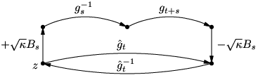
Let $t_{2}>t_{1}>0$ . We need to prove that $\gamma[0,t_{1}]\cap\gamma\left[{t_{2},\infty}\right)=\emptyset$ . To do so, note that there exists a rational $s\in(t_{1},t_{2})$ such that $\gamma(s)\not\in\mathbbm{R}\cup K_{t_{1}}$ , since the capacity is strictly increasing between $t_{1}$ and $t_{2}$ . In the following paragraphs we will prove that

\gamma\left[{s,\infty}\right)\cap(\mathbbm{R}\cup K_{s})=\{\gamma(s)\}.

(32)

Suppose for now that this is true, and assume that there is a point $z$ that is both in $\gamma[0,t_{1}]$ and in $\gamma\left[{t_{2},\infty}\right)$ . Then clearly $z\in\gamma\left[{s,\infty}\right)$ since $s<t_{2}$ , and $z\in\mathbbm{R}\cup K_{s}$ since $s>t_{1}$ . Hence $z=\gamma(s)$ by (32). But then it follows that $\gamma(s)=z\in\mathbbm{R}\cup K_{t_{1}}$ , a contradiction. This proves the theorem, so it only remains to establish (32).

To prove (32), for fixed $s$ as above consider the process $\hat{g}_{t}(z)$ defined by

\hat{g}_{t}(z):=g_{t+s}\big(g_{s}^{-1}(z+\sqrt{\kappa}B_{s})\big)-\sqrt{\kappa}B_{s}.

(33)

By stationarity of SLE (lemma 3.5), this process has the same distribution as $g_{t}(z)$ ; we saw in the derivation of the stationarity property that its driving process is $\sqrt{\kappa}(B_{t+s}-B_{s})$ . Let us denote by $\hat{\gamma}_{s}(t)$ the trace corresponding to the maps $\{\hat{g}_{t}:t\geq 0\}$ . Then we have

	$\displaystyle\hat{\gamma}_{s}(t)$	$\displaystyle:=$	$\displaystyle\hat{g}^{-1}_{t}\big(\sqrt{\kappa}(B_{t+s}-B_{s})\big)=g_{s}\big(g^{-1}_{t+s}(\sqrt{\kappa}B_{t+s})\big)-\sqrt{\kappa}B_{s}$		(34)
		$\displaystyle=$	$\displaystyle g_{s}\big(\gamma(t+s)\big)-\sqrt{\kappa}B_{s}$		(34)

as can be seen from figure 4. Applying the map $g^{-1}_{s}$ to this result gives

\gamma(t+s)=g^{-1}_{s}\big(\hat{\gamma}_{s}(t)+\sqrt{\kappa}B_{s}\big).

(35)

Now, lemma 4.2 tells us that for every $t\geq 0$ , $\hat{\gamma}_{s}(t)\in\mathbbm{H}\cup\{0\}$ . Hence, because $g^{-1}_{s}$ maps $\mathbbm{H}$ onto $H_{s}=\mathbbm{H}\setminus K_{s}$ , (32) follows. The proof is now complete. ∎

4.3 Locality and restriction

We discussed above the two special values of $\kappa$ where SLE undergoes a phase transition. Two other special values of $\kappa$ are $\kappa=6$ and $\kappa=8/3$ . At these values, $\mbox{SLE}_{\kappa}$ has some very specific properties, that will be discussed in detail below.

4.3.1 The locality property of $\mbox{SLE}_{6}$

Let us start by giving a precise definition of the locality property. Assume for now that $\kappa>0$ is fixed. Suppose that $L$ is a hull in $\mathbbm{H}$ which is bounded away from the origin. Let $K_{t}$ be the hulls of a chordal $\mbox{SLE}_{\kappa}$ process in $\mathbbm{H}$ , and let $K^{\ast}_{t}$ be the hulls of a chordal $\mbox{SLE}_{\kappa}$ process in $\mathbbm{H}\setminus L$ , both processes going from $0$ to $\infty$ . Denote by $T_{L}$ the first time at which $K_{t}$ intersects the set $L$ . Likewise, let $T^{\ast}_{L}$ be the first time when $K^{\ast}_{t}$ intersects $L$ (note that in this case, $T^{\ast}_{L}$ is the hitting time of an arc on the boundary of the domain). See figure 5 for an illustration comparing the traces of the two processes in their respective domains.

Chordal $\mbox{SLE}_{\kappa}$ is said to satisfy the locality property if for all hulls $L$ bounded away from the origin, the distribution of the hulls $\{K_{t}:t<T_{L}\}$ is the same as the distribution of the hulls $\{K^{\ast}_{t}:t<T^{\ast}_{L}\}$ , modulo a time re-parameterization. Loosely speaking, suppose that $\mbox{SLE}_{\kappa}$ has the locality property, and that we are only interested in the process up to the first time when it hits $L$ . Then it doesn’t matter whether we consider chordal $\mbox{SLE}_{\kappa}$ from $0$ to $\infty$ in the domain $\mathbbm{H}$ , or chordal $\mbox{SLE}_{\kappa}$ from $0$ to $\infty$ in the smaller domain $\mathbbm{H}\setminus L$ : up to a time-change, these processes are the same. It was first proved in [35] that chordal $\mbox{SLE}_{\kappa}$ has the locality property for $\kappa=6$ , and for no other values of $\kappa$ . Later, a much simpler proof appeared in [42]. A sketch of the proof with a discussion of some consequences appears in [33].

So far, we defined the locality property for a chordal process in $\mathbbm{H}$ , but it is clear that by conformal invariance we can translate the property to an arbitrary simply connected domain. It is also true that radial $\mbox{SLE}_{6}$ has the same property. We shall not go into this further, but we would like to point out one particular consequence of the locality property of $\mbox{SLE}_{6}$ .

Suppose that $D$ is a simply connected domain with continuous boundary, and let $a$ , $b$ and $b^{\prime}$ be three distinct points on the boundary of $D$ . Denote by $I$ the arc of $\partial D$ between $b$ and $b^{\prime}$ which does not contain $a$ (see figure 6 for an illustration). Let $K_{t}$ (respectively $K_{t}^{\prime}$ ) be the hulls of a chordal $\mbox{SLE}_{6}$ process from $a$ to $b$ (respectively $b^{\prime}$ ) in $D$ , and let $T$ (respectively $T^{\prime}$ ) be the first time when the process hits $I$ . Then modulo a time-change, $\{K_{t}:t<T\}$ and $\{K^{\prime}_{t}:t<T^{\prime}\}$ have the same distribution. As a consequence, if you are interested in the behaviour of an $\mbox{SLE}_{6}$ process up to the first time when it hits an arc $I$ , then you may choose any point of $I$ as the endpoint for the SLE process without affecting its behaviour.

4.3.2 The restriction property of $\mbox{SLE}_{8/3}$

To define the restriction property, assume that $\kappa\leq 4$ is fixed. Then the trace $\gamma$ of $\mbox{SLE}_{\kappa}$ is a simple path. Now suppose, as in our discussion of the locality property above, that $L$ is a hull in the half-plane which is bounded away from the origin. Let $\Psi$ be the map defined by $\Psi(z):=g_{L}(z)-g_{L}(0)$ . Then $\Psi$ is the unique conformal map of $\mathbbm{H}\setminus L$ onto $\mathbbm{H}$ such that $\Psi(0)=0$ , $\Psi(\infty)=\infty$ and $\Psi^{\prime}(\infty)=1$ . Now suppose that $\gamma$ never hits $L$ . Then we let $\gamma^{\ast}$ be the image of $\gamma$ under the map $\Psi$ , that is $\gamma^{\ast}(t):=\Psi(\gamma(t))$ .

We say that $\mbox{SLE}_{\kappa}$ has the restriction property if for all hulls $L$ that are bounded away from the origin, conditional on the event $\{\gamma\left[{0,\infty}\right)\cap L=\emptyset\}$ , the distribution of $\gamma^{\ast}\left[{0,\infty}\right)$ is the same as the distribution of the trace of a chordal $\mbox{SLE}_{\kappa}$ process in $\mathbbm{H}$ , modulo a time re-parameterization. In words, suppose that $\mbox{SLE}_{\kappa}$ has the restriction property. Then the distribution of all paths that are restricted not to hit $L$ , and which are generated by $\mbox{SLE}_{\kappa}$ in the half-plane, is the same as the distribution of all paths generated by $\mbox{SLE}_{\kappa}$ in the domain $\mathbbm{H}\setminus L$ .

SLE has the restriction property for $\kappa=8/3$ and for no other values of $\kappa$ . A proof is given in [42] (a sketch of a proof appears in [33]), and in the same article it was also shown that

\mbox{\boldmath P}\big[\gamma\left[{0,\infty}\right)\cap L=\emptyset\big]=|\Psi^{\prime}(0)|^{5/8}.

(36)

Again, the restriction property can be translated into a similar property for arbitrary domains, and radial $\mbox{SLE}_{8/3}$ also satisfies the restriction property. We refer to Lawler, Schramm and Werner [42] and Lawler [33] for more information.

4.4 Hausdorff dimensions

Consider an $\mbox{SLE}_{\kappa}$ process in the upper half-plane. If $\kappa\geq 8$ the trace of the process is space-filling, and therefore the Hausdorff dimension of the set $\gamma\left[{0,\infty}\right)$ is $2$ . But for $\kappa\in(0,8)$ the Hausdorff dimension of $\gamma\left[{0,\infty}\right)$ is a non-trivial number. Rohde and Schramm [51] showed that its value is bounded from above by $1+\kappa/8$ , and the proof that for $\kappa\neq 4$ the Hausdorff dimension is in fact $1+\kappa/8$ was completed by Beffara [11, 12]. In the physics literature the Hausdorff dimensions of the curves that are believed to converge to SLE were predicted by Duplantier and Saleur [18, 52].

In the case $\kappa>4$ the hull of $\mbox{SLE}_{\kappa}$ is not a simple path, and it is natural to consider also the Hausdorff dimension of the boundary of $K_{t}$ for some fixed value of $t>0$ . Its value is conjectured to be $1+2/\kappa$ , because (based on a duality relation derived by Duplantier [18]) it is believed that the boundary of the hull for $\kappa>4$ is described by $\mbox{SLE}_{16/\kappa}$ . The dimension of the hull boundary is known rigorously only for $\kappa=6$ (where it is $4/3$ ) and for $\kappa=8$ (where it is $5/4$ ). For $\kappa=6$ this follows from the study of the “conformal restriction measures” in [42], for $\kappa=8$ this is a consequence of the strong relation between loop-erased random walks and uniform spanning trees [40] (section 5.3).

5 SLE and discrete models

In this section we take a look at the connection between SLE and discrete models. The connection is made by defining a path in these discrete models, which in the scaling limit converges to the trace of a chordal or radial SLE process. In the first subsection, we describe how this works for the exploration process of critical percolation, which is known to converge to $\mbox{SLE}_{6}$ . Then we describe the harmonic explorer and its convergence to $\mbox{SLE}_{4}$ . In section 5.3 we consider the loop-erased random walk and the Peano curve associated with the uniform spanning tree. These paths converge to the traces of $\mbox{SLE}_{2}$ and $\mbox{SLE}_{8}$ respectively. Section 5.4 is about the conjectured connection between self-avoiding walks and $\mbox{SLE}_{8/3}$ . The final two subsections relate Potts models and O( $n$ )-model to their SLE counterparts.

5.1 Critical percolation

We define site percolation on the triangular lattice as follows. All vertices of the lattice are independently coloured blue with probability $p$ or yellow with probability $1-p$ . An equivalent, and perhaps more convenient, viewpoint is to say that we colour all hexagons of the dual lattice blue or yellow with probabilities $p$ and $1-p$ , respectively. It is well-known that for $p\leq 1/2$ , there is almost surely no infinite cluster of connected blue hexagons, while for $p>1/2$ there a.s. exist a unique infinite blue cluster. This makes $p=1/2$ the critical point for site percolation on the triangular lattice. For the remainder of this subsection we assume that we are at this critical point.

Let us for now restrict ourselves to the half-plane. Suppose that as our boundary conditions, we colour all hexagons intersecting the negative real line yellow, and all hexagons intersecting the positive real line blue. All other hexagons in the half-plane are independently coloured blue or yellow with equal probabilities. Then there exists a unique path over the edges of the hexagons, starting in the origin, which separates the cluster of blue hexagons attached to the positive real half-line from the cluster of yellow hexagons attached to the negative real half-line. This path is called the chordal exploration process from $0$ to $\infty$ in the half-plane. See figure 7 for an illustration.

The exploration process can also be described as the unique path from the origin such that at each step there is a blue hexagon on the right, and a yellow hexagon on the left. This path can also be generated dynamically, as follows. Initially, only the hexagons on the boundary receive a colour. Then after each step, the exploration process meets a hexagon. If this hexagon has not yet been coloured, we have to choose whether to make it blue or yellow, and the exploration process can turn left or right with equal probabilities. But if the hexagon has already been coloured blue or yellow, the exploration path is forced to turn left or right, respectively.

Note that in this dynamic formulation it is clear that the trajectory of the exploration process is determined completely by the colours of the hexagons in the direct vicinity of the path. Further, it is clear that the tip of the process can not become trapped, because it is forced to reflect off into the open if it meets an already coloured hexagon. This suggests that in the continuum limit, when we send the size of the hexagons to zero, the exploration process may be described by a Löwner evolution. The only candidate is $\mbox{SLE}_{6}$ , because only then we have the locality property.

Smirnov [56] proved that in the continuum limit, the exploration process is conformally invariant. Together with the results on $\mbox{SLE}_{6}$ developed by Lawler, Schramm and Werner, this should prove that the exploration process converges to the trace of $\mbox{SLE}_{6}$ in the half-plane (although explicit proofs linking $\mbox{SLE}_{6}$ to critical percolation have not yet appeared). Thus, $\mbox{SLE}_{6}$ may be used to calculate properties of critical percolation that can be formulated in terms of the behaviour of the exploration process. Some examples of how this can be done are described in section 6.

So far, we have restricted percolation to a half-plane, but we can of course consider other domains as well. For example, let $D$ be a simply connected domain with continuous boundary, and let $a$ and $b$ be two points on the boundary. In an approximation of the domain by hexagons, colour all hexagons that intersect the arc of $\partial D$ from $a$ to $b$ in the counter-clockwise direction blue, and all remaining hexagons intersecting $\partial D$ yellow. Then there is a unique exploration process in $D$ which goes from $a$ to $b$ , and by Smirnov’s result it converges in the scaling limit to a chordal $\mbox{SLE}_{6}$ trace in $D$ going from $a$ to $b$ . On that note we end our discussion of the connection between critical percolation and $\mbox{SLE}_{6}$ .

5.2 The harmonic explorer

The harmonic explorer is a random path similar to the exploration process of critical percolation. It was defined recently by Schramm and Sheffield as a discrete process that converges to $\mbox{SLE}_{4}$ [55]. To define the harmonic explorer, consider an approximation of a bounded domain with hexagons, as in figure 8. As we did for critical percolation, we partition the set of hexagons on the boundary of our domain into two components, and colour the one component yellow and the other blue. The hexagons in the interior are uncoloured initially.

The harmonic explorer is a path over the edges of the hexagons that starts out on the boundary with a blue hexagon on its right and a yellow hexagon on its left. It turns left when it meets a blue hexagon, and it turns right when it meets a yellow hexagon. The only difference with the exploration process of critical percolation is in the way the colour of an as yet uncoloured hexagon is determined. For the harmonic explorer this is done as follows.

Suppose that the harmonic explorer meets an uncoloured hexagon (see figure 8). Let $f$ be the function, defined on the faces of the hexagons, that takes the value $1$ on the blue hexagons, the value $0$ on the yellow hexagons, and is discrete harmonic on the uncoloured hexagons. Then the probability that the hexagon whose colour we want to determine is made blue, is given by the value of $f$ on this hexagon. Proceeding in this way, we obtain a path crossing the domain between the two points on the boundary where the blue and yellow hexagons meet. In the scaling limit this path converges to the trace of chordal $\mbox{SLE}_{4}$ .

5.3 Loop-erased random walks and uniform spanning trees

In this subsection we consider loop-erased random walks (LERW’s) and uniform spanning trees (UST’s). We shall define both models first, and we will point out the close relation between the two. Then we will discuss the connection with SLE in the scaling limit. Schramm [53] already proved that the LERW converges to $\mbox{SLE}_{2}$ under the assumption that the scaling limit exists and is conformally invariant. In the same work, he also conjectured the relation between UST’s and $\mbox{SLE}_{8}$ . The final proofs of these connections were given by Lawler, Schramm and Werner in [40]. Their proofs hold for general lattices, but for simplicity, we shall restrict our description here to finite subgraphs of the square grid $\delta\mathbbm{Z}^{2}$ with mesh $\delta>0$ .

Suppose that $G$ is a finite connected subgraph of $\delta\mathbbm{Z}^{2}$ , let $u$ be a vertex of $G$ and let $V$ be a collection of vertices of $G$ not containing $u$ . Then the LERW from $u$ to $V$ in $G$ is defined by taking a simple random walk in $G$ from $u$ to $V$ and erasing all its loops in chronological order. More precisely, if $\big(\omega(0),\ldots,\omega(T_{V})\big)$ are the vertices visited by a simple random walk starting from $u$ and stopped at the first time $T_{V}$ when it visits a vertex in $V$ , then its loop-erasure $\big(\beta(0),\ldots,\beta(T)\big)$ is defined as follows. We start by setting $\beta(0)=\omega(0)$ . Then for $n\in\mathbbm{N}$ we define inductively: if $\beta(n)\in V$ then $T=n$ and we are done, and otherwise we set $\beta(n+1)=\omega(1+\max\{m\leq T_{V}:\omega(m)=\beta(n)\})$ . The path $\big(\beta(0),\ldots,\beta(T)\big)$ is then a sample of the LERW in $G$ from $u$ to $V$ .

A spanning tree $T$ in $G$ is a subgraph of $G$ such that every two vertices of $G$ are connected via a unique simple path in $T$ . A uniform spanning tree (UST) in $G$ is a spanning tree chosen with the uniform distribution from all spanning trees in $G$ . It is well-known that the distribution of the unique simple path connecting two distinct vertices $u$ and $v$ of $G$ in the UST is the same as that of the LERW from $u$ to $\{v\}$ in $G$ .

In fact, the connection between LERW’s and UST’s is even stronger. For suppose that we fix an ordering $(v_{0},\ldots,v_{n})$ of the vertices in $G$ . Let $T_{0}=\{v_{0}\}$ and inductively define $T_{m+1}$ as the union of $T_{m}$ and a LERW from $v_{m+1}$ to $T_{m}$ , $T_{m+1}=T_{m}$ if $v_{m+1}\in T_{m}$ . Then $T_{n}$ is a UST in $G$ , regardless of the chosen ordering of the vertices of $G$ . This algorithm for generating UST’s from LERW’s is known as Wilson’s algorithm [60]. See also [40, 53] and references therein for more information.

Let us now describe the scaling limit of the LERW and the connection with SLE. We shall work with a fixed, bounded, simply connected domain $D$ . Fix the mesh $\delta>0$ , and let $G$ be the subgraph of $\delta\mathbbm{Z}^{2}$ consisting of all vertices and edges that are contained in $D$ . Then the set of all points that are disconnected from $\infty$ by $G$ is a discrete approximation $D^{\prime}$ of the domain $D$ , see figure 9, part (a). Suppose that $a$ is a fixed interior point of $D$ and let $u$ be the vertex of $G$ which is closest to $a$ . Consider the LERW on $\delta\mathbbm{Z}^{2}$ from $u$ to the set of vertices that are not in $G$ . In the scaling limit, the time-reversal of this LERW converges to the trace of a radial $\mbox{SLE}_{2}$ process in $D$ from $\partial D$ to $a$ . Here, the starting point of the $\mbox{SLE}_{2}$ process is defined by choosing the starting point of the Brownian motion driving the Löwner evolution on the unit disk uniformly on the unit circle.

The fact that the LERW converges to an $\mbox{SLE}_{2}$ process proves that the LERW is conformally invariant in the scaling limit. Because of the close connection between LERW’s and UST’s, this leads to the conclusion that the UST has a conformally invariant scaling limit as well. Moreover, we can define a path associated to the UST, that converges in the scaling limit to the trace of $\mbox{SLE}_{8}$ . This path is called the UST Peano curve, and can be defined as we describe below (figure 9 provides an illustration).

Consider again the domains $D$ , $D^{\prime}$ and graph $G$ as before. This time, let $b$ and $c$ be distinct points of $\partial D$ , and let $v$ and $w$ be distinct vertices of $G$ on $\partial D^{\prime}$ closest to $b$ and $c$ , respectively. We denote by $I$ the counter-clockwise arc from $v$ to $w$ of $\partial D^{\prime}$ , and identify all vertices of $G$ that are on $I$ . Now let $G^{\prime}$ be the graph consisting of all edges (and corresponding vertices) of the lattice dual to $\delta\mathbbm{Z}^{2}$ , that intersect edges of $G$ but not $I$ . Then we define the dual graph $G^{\dagger}$ of $G$ as the union of $G^{\prime}$ and those edges (and corresponding vertices) outside $D^{\prime}$ needed to connect the vertices of $G^{\prime}$ outside $D^{\prime}$ via the shortest possible path outside $D^{\prime}$ , see figure 9, part (b). On this dual graph, we identify all vertices that lie outside $D^{\prime}$ .

Now suppose that $T$ is a UST in $G$ . Then there is a dual tree $T^{\dagger}$ in $G^{\dagger}$ , consisting of all those edges that do not intersect edges of the tree $T$ , see figure 9, part (c). Observe that $T^{\dagger}$ is a UST in $G^{\dagger}$ . The Peano curve is defined as the curve winding between $T$ and $T^{\dagger}$ on the square lattice with vertices at the points $\frac{\delta}{2}\mathbbm{Z}^{2}+(\frac{\delta}{4},\frac{\delta}{4})$ . Note that this curve is space-filling, in that it visits all vertices of the lattice that are disconnected from $\infty$ by $G\cup G^{\dagger}$ . In the scaling limit, the Peano curve defined as above converges to the trace of a chordal $\mbox{SLE}_{8}$ process from $b$ to $c$ in $D$ .

5.4 Self-avoiding walks

A self-avoiding walk (SAW) of length $n$ on the square lattice $\delta\mathbbm{Z}^{2}$ with mesh $\delta>0$ is a nearest-neighbour path $\omega=\big(\omega(0),\omega(1),\ldots,\omega(n)\big)$ on the vertices of the lattice, such that no vertex is visited more than once. In this subsection we shall restrict ourselves to SAW’s that start in the origin and stay in the upper half-plane afterwards. The idea is to define a stochastic process, called the half-plane infinite SAW, that in the scaling limit $\delta\mathrel{\downarrow}0$ is believed to converge to chordal $\mbox{SLE}_{8/3}$ .

Following [41] we write $\Lambda_{n}^{+}$ for the set of all SAW’s $\omega$ of length $n$ that start in the origin, and stay above the real line afterwards. For a given $\omega$ in $\Lambda_{n}^{+}$ , let $Q_{k}^{+}(\omega)$ be the fraction of walks $\omega^{\prime}$ in $\Lambda_{n+k}^{+}$ whose beginning is $\omega$ , i.e. such that $\omega^{\prime}(i)=\omega(i)$ for $0\leq i\leq n$ . Define $Q^{+}(\omega)$ as the limit of $Q_{k}^{+}(\omega)$ as $k\mathrel{\rightarrow}\infty$ . Then $Q^{+}(\omega)$ is roughly the fraction of very long SAW’s in the upper half-plane whose beginning is $\omega$ . It was shown by Lawler, Schramm and Werner that the limit $Q^{+}(\omega)$ exists [41].

Now we can define the half-plane infinite self-avoiding walk as the stochastic process $X_{i}$ such that for all $\omega=\big(0,\omega(1),\ldots,\omega(n)\big)\in\Lambda^{+}_{n}$ ,

\mbox{\boldmath P}[X_{0}=0,X_{1}=\omega(1),\ldots,X_{n}=\omega(n)]=Q^{+}(\omega).

(37)

We believe that the scaling limit of this process as the mesh $\delta$ tends to $0$ exists and is conformally invariant. By the restriction property the scaling limit has to be $\mbox{SLE}_{8/3}$ , as pointed out in [41]. At this moment it is unknown how the existence, let alone the conformal invariance, of the scaling limit could be proved. However, there is very strong numerical evidence for the conformal invariance of the scaling limit of self-avoiding walks [27, 28], confirming the SLE predictions of its restriction property.

Lawler, Schramm and Werner [41] also explain how one can define a natural measure on SAW’s with arbitrary starting points, leading to conjectures relating SAW’s to chordal and radial $\mbox{SLE}_{8/3}$ in bounded simply-connected domains. The article further discusses similar conjectures for self-avoiding polygons, and predictions for the critical exponents of SAW’s that can be obtained from SLE. We shall not go into these topics here.

5.5 The Potts model

So far in this section we discussed relations between SLE at specific values of $\kappa$ to certain statistical lattice models. The results of SLE however suggest a further connection to continuous families of models, of which we will discuss the two most obvious examples in this and the following subsection. This subsection deals with the $q$ -state Potts model. Below we will show a standard treatment [10], which relates the partition sum of the Potts model to an ensemble of multiple paths on the lattice. In the scaling limit these paths will be the candidates for the SLE processes. The second example, allowing a similar treatment, is the O( $n$ ) model. This model will be discussed in the following subsection.

The Potts model has on each site of a lattice a variable $s_{j}$ which can take values in $\{1,2,\ldots,q\}$ . Of these variables only nearest neighbours interact such that the energy is $-1$ if both variables are in the same state and $0$ otherwise. The canonical partition sum is

Z=\sum_{\{s\}}\exp\left(\beta\sum_{\langle j,k\rangle}\delta_{s_{j},s_{k}}\right).

(38)

The summation in the exponent is over all nearest-neighbour pairs of sites, and the external summation over all configurations of the $s_{j}$ . The model is known to be disordered at high temperatures, and ordered at low temperatures. One of the signatures of order is that the probability that two distant $s$ -variables are in the same state does not decay to zero with increasing distance. We are interested in the behaviour at the transition.

In order to make the connection with a path on the lattice, we express this partition sum in a high-temperature expansion, i.e. in powers of a parameter which is small when $\beta$ is small. The first step is to write the summand as a product:

Z=\sum_{\{s\}}\prod_{\langle j,k\rangle}\left[1+({\rm e}^{\beta}-1)\delta_{s_{j},s_{k}}\right].

(39)

The product can be expanded in terms in which at every edge of the lattice a choice is made between the two terms $1$ and $({\rm e}^{\beta}-1)\delta_{s_{j},s_{k}}$ . In a graphical notation we place a bond on every edge of the lattice where the second term is chosen, see figure 10. For each term in the expansion of the product the summation over the $s$ -variables is trivial: if two sites are connected by bonds, their respective $s$ -variables take the same value, and are independent otherwise. As a result the summation over $\{s\}$ results in a factor $q$ for each connected component of the graph. Hence

Z=\sum_{{\rm graphs}}({\rm e}^{\beta}-1)^{b}q^{c},

(40)

where $c$ is the number of connected components of the graph and $b$ the number of bonds. This expansion is known by the name of Fortuin-Kasteleyn [22] cluster model. Note that, while $q$ has been introduced as the (integer) number of states, in this expansion it can take any value.

It is convenient to rewrite the graph expansion into an expansion of paths on a new lattice. The edges of the original lattice correspond to the vertices of the new lattice. The graphs on the original lattice are rewritten into polygon decompositions of the new lattice. Every vertex of the new lattice is separated into two non-intersecting path segments. These path segments intersect the corresponding edge of the original lattice if and only if this edge does not carry a bond of the graph, as follows:

As a result of these transformations the new lattice is decomposed into a collection of non-intersecting paths, as indicated in figure 10. Notice that every component of the original graph is surrounded by one of these closed paths, but also the closed circuits of the graph are inscribed by these paths. By Euler’s relation the number of components $c$ of the original graph can be expressed in the number of bonds $b$ , the total number of sites $N$ and the number of polygons $p$ : $c=(N-b+p)/2$ . An alternative expression for the partition sum is then

Z=\sum_{{\rm graphs}}\left(\frac{{\rm e}^{\beta}-1}{\sqrt{q}}\right)^{b}q^{(N+p)/2}.

(41)

At the critical point $\beta_{c}$ the relation $\exp(\beta_{c})=1+\sqrt{q}$ holds, so that the partition sum simplifies.

We will now consider this model at the critical point on a rectangular domain. The lattice approximation of this domain is chosen such that the lower-left corner of the rectangle coincides with a site of the lattice, while the upper-right corner coincides with a site of the dual lattice. The sides of the rectangle are parallel to the edges of the lattice, as in figure 10. We choose as boundary condition that all edges that are contained in the left and lower sides of the rectangle carry bonds, and all edges that intersect the right and upper sides perpendicularly carry no bonds. For the spin variables this means that all the spins on the left and lower sides are in the same state, while all other spins are unconstrained.

In such an arrangement the diagrams in (41) include one path from the lower-right to the upper-left corner. All further paths are closed polygons, see figure 10. We take the scaling limit by covering the same domain with a finer and finer mesh. It is believed [51] that in the scaling limit the measure on the paths approaches that of chordal $\mbox{SLE}_{\kappa}$ traces. From e.g. the Hausdorff dimension [12, 52] the relation between $\kappa$ and $q$ is

q=2+2\cos(8\pi/\kappa)

(42)

where $4\leq\kappa\leq 8$ . Only in a few cases this relation between $\mbox{SLE}_{\kappa}$ and the Potts partition sum has been made rigorous. For instance, in the limit $q\to 0$ , the graph expansion reduces to the uniform spanning tree, which has $\mbox{SLE}_{8}$ as its scaling limit.

5.6 The O( $n$ ) model

We now turn to the O( $n$ ) model, which is another well-known model where a high-temperature expansion results in a sum over paths. Here the dynamic variables are $n$ -component vectors of a fixed length, and the Hamiltonian is invariant under rotations in the $n$ -dimensional space. The simplest high-temperature expansion is obtained when the Boltzmann weight is chosen as

\prod_{\langle j,k\rangle}(1+xs_{i}\cdot s_{j}),

(43)

where the product is over nearest neighbours on a hexagonal lattice. The partition sum is obtained by integrating this expression over the directions of the spin vectors. Like for the Potts model one can expand the product and do the bookkeeping of the terms by means of graphs. In each factor in (43) the choice of the second term is indicated by a bond. Then the graphs that survive the integration over the spin variables have only even vertices, i.e. on the hexagonal lattice vertices with zero or two bonds. As a result the graphs consist of paths on the lattice. In a well-chosen normalization of the measure and the length of the spins, the partition sum is a sum over even graphs

Z=\sum_{\rm graphs}x^{L}n^{M},

(44)

where $M$ is the number of closed loops, and $L$ their combined length. Note that this expression for the partition sum is well-defined also when the number of spin components $n$ is not integer. It is known [9, 45] that the critical point is at $x_{c}=[2+(2-n)^{1/2}]^{-1/2}$ for $0\leq n\leq 2$ . When $x$ is larger that this critical value, the model also shows critical behaviour.

Consider now this model on a bounded domain, and take a correlation function between two spins on the boundary. The diagrams that contribute to this function contain one path between the two specified boundary points and any number of closed polygons in the interior. We conjecture that at the critical value of $x$ in the scaling limit the measure on the paths between the two boundary spins approaches that of chordal $\mbox{SLE}_{\kappa}$ for $n=-2\cos(4\pi/\kappa)$ and $8/3\leq\kappa\leq 4$ . For larger values of $x$ , the scaling limit would again be $\mbox{SLE}_{\kappa}$ , with the same relation between $\kappa$ and $n$ , but now with $4\leq\kappa\leq 8$ .

To conclude this section, we remark that the same partition sum (44) can also be viewed as the partition sum of a dilute Potts model on the triangular lattice, described in [47]. In this variant of the Potts model the spins take values in $\{0,1,2,\ldots,q\}$ . The model is symmetric under permutations of the $q$ positive values. The name dilute comes from the interpretation of the neutral value $0$ as a vacant site. If neighbouring sites take different values, then one of them takes the value $0$ . The Boltzmann weight is a product over the elementary triangles of weights that depend on the three sites at the corners of the triangle. We take this weight to be $1$ when all three sites are in the same state, vacant or otherwise. Triangles with one or two vacant sites have weights $xy$ and $x/y$ , respectively. The partition sum can be expanded in terms of domain walls between sites of different values. This expansion takes the form of (44) for $y^{12}=q=n^{2}$ , which is the locus of the phase transition between an ordered phase and a disordered phase. Within this locus, the region with $x>x_{c}$ is a second-order transition. In the regime $x<x_{c}$ the transition is discontinuous, and the position $x=x_{c}$ separates the two regimes and is called the tricritical point. When $q=x=1$ the site percolation problem on the triangular lattice is recovered, which is known to converge to $\mbox{SLE}_{6}$ in the scaling limit.

6 SLE computations and results

In this section we discuss some of the results that have been obtained from calculations involving SLE processes. Our aim in this section is not only to provide an overview of these results, but also to give an impression of the typical SLE computations involved, using techniques from stochastic calculus and conformal mapping theory.

This section is organized as follows. In the first subsection we discuss several SLE calculations independently from their connection with other models. The results we obtain will be key ingredients for further calculations. The second subsection gives a brief overview of how SLE can be applied to calculate the intersection exponents of Brownian motion. Finally, we will discuss results on critical percolation that have been obtained from its connection with $\mbox{SLE}_{6}$ .

6.1 Several SLE calculations

The purpose of this subsection is to explain how some typical probabilities and corresponding exponents of events involving chordal SLE processes can be calculated. The results we find in this subsection are for whole ranges of $\kappa$ , and might therefore have applications in various statistical models. Some typical applications of the results for $\kappa=6$ will be shown in the following subsections.

6.1.1 The one-sided crossing exponent

Consider a chordal $\mbox{SLE}_{\kappa}$ process inside the rectangle $\mathcal{R}_{L}:=(0,L)\times(0,{\rm i}\pi)$ , which goes from ${\rm i}\pi$ to $L$ . If $\kappa>4$ this process will at some random time $\tau$ hit the right edge $[L,L+{\rm i}\pi]$ of the rectangle, as in figure 11. Suppose that $E$ denotes the event that up to this time $\tau$ , the SLE process has not hit the lower edge of the rectangle. Then the following holds.

Theorem 6.1

The $\mbox{SLE}_{\kappa}$ process as described above satisfies, for $\kappa>4$ ,

\mbox{\boldmath P}[E]\asymp\exp\left[-\big(1-\frac{4}{\kappa}\big)L\right]\quad\mbox{as\ }L\mathrel{\rightarrow}\infty,

(45)

where $\asymp$ indicates that each side is bounded by some constant times the other side.

Proof.

The proof we present here is a simplification of the proof of a more general result which appears in [35] and which we shall discuss below. To prove the theorem, the problem is first translated to the upper half-plane. So, let $\Psi:\mathcal{R}_{L}\mathrel{\rightarrow}\mathbbm{H}$ be the conformal map such that $\Psi(0)=1$ , $\Psi(L)=\infty$ and $\Psi(L+{\rm i}\pi)=0$ . Then the number $\xi:=\Psi({\rm i}\pi)\in(0,1)$ is determined uniquely. This map is just the map of corollary A.14 in appendix A.5, and from this we know that $\xi\uparrow 1$ as we send $L$ to infinity.

Let $K_{t}$ be the hulls of a chordal $\mbox{SLE}_{\kappa}$ process in the upper half-plane, which is translated over the distance $\xi$ to make it start in $\xi$ , and let $\gamma(t)$ denote the trace of the process. Set

$\displaystyle T_{0}$	$\displaystyle:=$	$\displaystyle\inf\big\{t\geq 0:\gamma(t)\in\left({-\infty,0}\right]\big\};$	(46)
$\displaystyle T_{1}$	$\displaystyle:=$	$\displaystyle\inf\big\{t\geq 0:\gamma(t)\in\left[{1,\infty}\right)\big\};$	(47)
$\displaystyle T_{\phantom{1}}$	$\displaystyle:=$	$\displaystyle\min\{T_{0},T_{1}\}.$	(48)

Then $T_{0}$ corresponds to the time $\tau$ when the process first crosses the rectangle, and $T_{1}$ corresponds to the first time at which the process hits the bottom edge of the rectangle. Hence, the event $E$ of the theorem translates to the event $\{T_{0}<T_{1}\}$ . Refer to figure 11 for an illustration.

Now we are going to define a process which allows us to determine whether the event $\{T_{0}<T_{1}\}$ or its complement occurs. A good candidate for such a process is the process $Z_{t}$ given by

Z_{t}:=\frac{W_{t}-g_{t}(0)}{g_{t}(1)-g_{t}(0)},\quad 1-Z_{t}=\frac{g_{t}(1)-W_{t}}{g_{t}(1)-g_{t}(0)}

(49)

where $W_{t}$ denotes the driving process of the Löwner evolution, i.e. $W_{t}$ is Brownian motion multiplied by $\sqrt{\kappa}$ , and $W_{0}=\xi$ .

Indeed, at time $T$ either the point $0$ or the point $1$ becomes part of the hull. In the first case, $\lim_{t\mathrel{\uparrow}T}Z_{t}=0$ because $\lim_{t\mathrel{\uparrow}T}(g_{t}(0)-W_{t})=0$ , whereas in the second case $\lim_{t\mathrel{\uparrow}T}Z_{t}=1$ , since $\lim_{t\mathrel{\uparrow}T}(g_{t}(1)-W_{t})=0$ . It is further clear that for all $t<T$ , $W_{t}\in(g_{t}(0),g_{t}(1))$ , implying that $Z_{t}\in(0,1)$ for all $t<T$ . This means that the stopping time $T$ conveniently translates into a stopping time for $Z_{t}$ , namely into the first time when $Z_{t}$ hits $0$ or $1$ . The value of $Z_{t}$ at this stopping time tells us whether the event $\{T_{0}<T_{1}\}$ occurs.

We now derive the differential equation for $Z_{t}$ , using stochastic calculus. First observe that

	$\displaystyle{\rm d}{[W_{t}-g_{t}(0)]}={\rm d}{W_{t}}-\frac{2\,{\rm d}{t}}{g_{t}(0)-W_{t}},$		(50)
	$\displaystyle{\rm d}{[g_{t}(1)-g_{t}(0)]}=\frac{2\,{\rm d}{t}}{g_{t}(1)-W_{t}}-\frac{2\,{\rm d}{t}}{g_{t}(0)-W_{t}}.$		(51)

Therefore, Itô’s formula (theorem B.11) tells us that $Z_{t}$ satisfies

$\displaystyle{\rm d}{Z_{t}}$	$\displaystyle=$	$\displaystyle\frac{2{\rm d}{t}}{(g_{t}(1)-g_{t}(0))^{2}}\left(\frac{g_{t}(1)-g_{t}(0)}{W_{t}-g_{t}(0)}-\left[\frac{W_{t}-g_{t}(0)}{g_{t}(1)-W_{t}}+1\right]\right)$	(52)
		$\displaystyle\hbox{}-\frac{{\rm d}{W_{t}}}{g_{t}(1)-g_{t}(0)}$
	$\displaystyle=$	$\displaystyle\frac{2\,{\rm d}{t}}{(g_{t}(1)-g_{t}(0))^{2}}\left(\frac{1}{Z_{t}}-\frac{1}{1-Z_{t}}\right)-\frac{{\rm d}{W_{t}}}{g_{t}(1)-g_{t}(0)}.$

If we now re-parameterize time by introducing the new time parameter

s=s(t):=\int_{0}^{t}\frac{{\rm d}{t}}{(g_{t}(1)-g_{t}(0))^{2}}\quad\mbox{for\ }t<T,

(53)

with the inverse $t(s)$ , then it is clear that the process $\tilde{Z}_{s}:=Z_{t(s)}$ satisfies

{\rm d}{\tilde{Z}_{s}}={\rm d}{X_{s}}+\left(\frac{2}{\tilde{Z}_{s}}-\frac{2}{1-\tilde{Z}_{s}}\right){\rm d}{s}={\rm d}{X_{s}}+\frac{2(1-2\tilde{Z}_{s})}{\tilde{Z}_{s}(1-\tilde{Z}_{s})}\,{\rm d}{s},

(54)

where $X_{s}$ has the same distribution as the process $W_{t}$ , i.e. it is a Brownian motion multiplied by the factor $\sqrt{\kappa}$ and starts in $\xi$ (theorem B.12).

From the above calculation we conclude that the process $\tilde{Z}_{s}$ is a time-homogeneous Markov process. As we explained earlier, we are interested in the value of this process at the stopping time $s(T):=\lim_{t\mathrel{\uparrow}T}s(t)$ , which is the first time when $\tilde{Z}_{s}$ hits $0$ or $1$ . To be more precise, we want to calculate

f(\xi):=\mbox{\boldmath E}\big[1_{\displaystyle\{\tilde{Z}_{s(T)}=0\}}\mathrel{\big|}\tilde{Z}_{0}=\xi\big]

(55)

where we take the expectation with respect to the Markov process started from $\tilde{Z}_{0}=\xi$ . Observe that the event $\{\tilde{Z}_{s(T)}=0\}$ is equivalent to the event $\{T_{0}<T_{1}\}$ .

Since $\tilde{Z}_{s}$ is a time-homogeneous Markov process, the process $Y_{s}:=f(\tilde{Z}_{s})$ (conditioned on $s<s(T)$ ) is a martingale with respect to the Brownian motion (theorem B.7). Hence, the drift term in its Itô formula must vanish at $s=0$ . It follows that $f(\xi)$ must satisfy the differential equation

\frac{\kappa}{2}\xi(1-\xi)f^{\prime\prime}(\xi)+2(1-2\xi)f^{\prime}(\xi)=0.

(56)

The boundary conditions are clearly given by $f(0)=1$ and $f(1)=0$ . The solution can be written as

f(\xi)=\frac{2^{1-\frac{8}{\kappa}}\,\Gamma\left(\frac{3}{2}-\frac{4}{\kappa}\right)}{\sqrt{\pi}\,\Gamma\left(2-\frac{4}{\kappa}\right)}(1-\xi)^{1-\frac{4}{\kappa}}\,\hbox{}_{2}F_{1}\left(1-\frac{4}{\kappa},\frac{4}{\kappa};2-\frac{4}{\kappa};1-\xi\right).

(57)

For critical percolation ( $\kappa=6$ ) this is Cardy’s formula [15]. Note that $f(\xi)$ is exactly the probability $\mbox{\boldmath P}[E]$ , and that the relation between $\xi$ and $L$ is given by the conformal mapping of corollary A.14. Hence, we have basically found the probability $\mbox{\boldmath P}[E]$ as a function of $L$ . The asymptotic behaviour follows from $1-\xi=\exp[-L+O(1)]$ (corollary A.14) and the observation that $f(\xi)(1-\xi)^{4/\kappa-1}$ is bounded from above and below by some constants when $\xi\mathrel{\uparrow}1$ (consult e.g. [48] for more information on the behaviour of the hypergeometric function). ∎

We can generalize the theorem in the following way. Consider again an $\mbox{SLE}_{\kappa}$ process crossing the rectangle $\mathcal{R}_{L}$ from ${\rm i}\pi$ to $L$ . On the event $E$ the trace $\gamma$ has crossed the rectangle without hitting the bottom edge. So conditional on this event, the $\pi$ -extremal distance between $[0,{\rm i}\pi]$ and $[L,L+{\rm i}\pi]$ in $\mathcal{R}_{L}\setminus K_{\tau}$ is well-defined. Let us call this $\pi$ -extremal distance $\mathcal{L}$ . Then one can prove the following generalization of theorem 6.1.

Theorem 6.2

For any $\lambda\geq 0$ and $\kappa>4$ ,

\mbox{\boldmath E}[1_{E}\,{\rm e}^{-\lambda\mathcal{L}}]\asymp\exp\big[-u(\kappa,\lambda)L]\qquad\mbox{as\ }L\mathrel{\rightarrow}\infty,

(58)

where

u(\kappa,\lambda)=\lambda+\frac{\kappa-4+\sqrt{(\kappa-4)^{2}+16\kappa\lambda}}{2\kappa}.

(59)

The exponent $u(\kappa,\lambda)$ is called the one-sided crossing exponent, because it measures the extremal distance on one side of an SLE process crossing a rectangle. Observe that $u(\kappa,\lambda)$ reduces to the exponent $1-4/\kappa$ for $\lambda=0$ as it should, because in this case theorem 6.2 is completely analogous to theorem 6.1. The derivation of the one-sided crossing exponent in [35] is rather involved, so we give only a sketch of the proof here.

Sketch of the proof of theorem 6.2

We use the same notations as in the proof of theorem 6.1. Suppose that we define the conformal maps $f_{t}(z)$ for $t<T$ by

f_{t}(z)=\frac{g_{t}(z)-g_{t}(0)}{g_{t}(1)-g_{t}(0)}.

(60)

This is a renormalized version of $g_{t}$ that fixes the points $0$ , $1$ and $\infty$ . Now turn back to figure 11 once more, and let $M_{T}:=\sup\{K_{T}\cap\mathbbm{R}\}$ . If we set $N_{T}:=f_{T}(M_{T})$ then it should be clear from conformal invariance that the $\pi$ -extremal distance $\mathcal{L}$ just translates into the $\pi$ -extremal distance between the intervals $\left({-\infty,0}\right]$ and $[N_{T},1]$ in the upper half-plane.

By corollary A.14 in appendix A.5, this $\pi$ -extremal distance satisfies

\mathcal{L}=-\log[1-N_{T}]+O(1)

(61)

and it follows that we have to determine the expectation value of the random variable $(1-N_{T})^{\lambda}$ on the event $E$ . Set $x:=1-\xi$ . Then we claim that the value of $(1-N_{T})$ is comparable to $xf^{\prime}_{T}(1)$ . This can be made more precise, see [35] for the details. It follows that it is sufficient to calculate the expectation value of $1_{E}f^{\prime}_{T}(1)^{\lambda}$ .

The calculation proceeds by setting $\alpha_{s}:=\log f^{\prime}_{t(s)}(1)$ for $s<s(T)$ , where the time re-parameterization is the same as in the proof of theorem 6.1. With Itô’s formula one can then calculate $\partial_{s}\alpha_{s}$ , which turns out to depend only on $\tilde{Z}_{s}$ . Therefore, $(\tilde{Z}_{s},\alpha_{s})$ is a two-dimensional time-homogeneous Markov process. So if we set

y(\xi,v):=\mbox{\boldmath E}\Big[1_{\displaystyle\{\tilde{Z}_{s(T)}=0\}}\,{\rm e}^{\lambda\alpha_{s(T)}}\mathrel{\Big|}\tilde{Z}_{0}=\xi,\alpha_{0}=v\Big],

(62)

then $y(\tilde{Z}_{s},\alpha_{s})$ is a martingale, and $y(\xi,0)$ is the expectation value we are trying to calculate. Itô’s formula again yields a differential equation for $y(\xi,v)$ , and this equation can be solved to find the value of the one-sided crossing exponent. $\Box$

6.1.2 The annulus crossing exponent

There is an analogue of the one-sided crossing exponent for radial SLE, which we shall discuss only briefly here. The setup is as follows. We consider radial $\mbox{SLE}_{\kappa}$ for any $\kappa>0$ , and set $A_{t}:=\partial\mathbbm{D}\setminus K_{t}$ . Then the set $A_{t}$ is either a piece of arc of the unit circle, or $A_{t}=\emptyset$ . Let $r>0$ and let $T(r)$ be the first time when the SLE process hits the circle $\{z:|z|=r\}$ . Denote by $E$ the event that $A_{T(r)}$ is non-empty. On the event $E$ , let $\mathcal{L}$ be the $\pi$ -extremal distance between the circles $\{z:|z|=1\}$ and $\{z:|z|=r\}$ in $\mathbbm{D}\setminus K_{T(r)}$ , see figure 12.

Theorem 6.3

For all $\lambda>0$ and $\kappa>0$ ,

\mbox{\boldmath E}[1_{E}\,{\rm e}^{-\lambda\mathcal{L}}]\asymp r^{-\nu(\kappa,\lambda)}\qquad{\rm as\ }r\mathrel{\downarrow}0,

(63)

where

\nu(\kappa,\lambda)=\frac{8\lambda+\kappa-4+\sqrt{(\kappa-4)^{2}+16\kappa\lambda}}{16}.

(64)

We call $\nu(\kappa,\lambda)$ the annulus crossing exponent of $\mbox{SLE}_{\kappa}$ . A detailed proof of the theorem can be found in [36]. It proceeds along the same lines as the proof of the one-sided crossing exponent.

6.1.3 Left-passage probability of SLE

So far, we have considered several crossing events of SLE processes. A different kind of event, namely the event that the trace of SLE passes to the left of a given point $z_{0}$ , was studied by Schramm in [54]. We shall reproduce his computation of the probability of this event below.

Theorem 6.4

Let $\kappa\in\left[{0,8}\right)$ and $z_{0}=x_{0}+{\rm i}y_{0}\in\mathbbm{H}$ . Suppose that $E$ is the event that the trace $\gamma$ of chordal $\mbox{SLE}_{\kappa}$ passes to the left of $z_{0}$ . Then

\mbox{\boldmath P}[E]={\frac{1}{2}}+\frac{\Gamma\left(\frac{4}{\kappa}\right)}{\sqrt{\pi}\,\Gamma\left(\frac{8-\kappa}{2\kappa}\right)}\,\hbox{}_{2}F_{1}\left({\frac{1}{2}},\frac{4}{\kappa};\frac{3}{2};-\frac{x_{0}^{2}}{y_{0}^{2}}\right)\frac{x_{0}}{y_{0}}.

(65)

Proof.

Define $X_{t}:=\mathop{\rm Re\,}\nolimits g_{t}(z_{0})-\sqrt{\kappa}B_{t}$ , $Y_{t}:=\mathop{\rm Im\,}\nolimits g_{t}(z_{0})$ and set $Z_{t}:=X_{t}/Y_{t}$ . As before, we let $\tau(z_{0})$ be the first time when the point $z_{0}$ is in the hull of $\mbox{SLE}_{\kappa}$ (for $\kappa\leq 4$ this never happens, so then $\tau(z_{0})=\infty$ ). We consider $\gamma$ up to the time $\tau(z_{0})$ only.

Suppose that $\omega(z_{0},t)$ is the harmonic measure of the union of $\left[{0,\infty}\right)$ and the right-hand side of $\gamma\left[{0,t}\right)$ at the point $z_{0}$ in the domain $H_{t}=\mathbbm{H}\setminus K_{t}$ . Then on the event $E$ , i.e. when $\gamma$ is to the left of $z_{0}$ , $\omega(z_{0},t)$ tends to $1$ when $t\mathrel{\uparrow}\tau(z_{0})$ . To see this, note that in this limit a Brownian motion started from $z_{0}$ is certain to first exit the domain $H_{t}$ through the union of $\left[{0,\infty}\right)$ and the right-hand side of $\gamma\left[{0,t}\right)$ , see figure 13. By conformal invariance of harmonic measure, it follows that the harmonic measure of $\left[{\sqrt{\kappa}B_{t},\infty}\right)$ at the point $g_{t}(z_{0})$ with respect to $\mathbbm{H}$ tends to $1$ when $t\mathrel{\uparrow}\tau(z_{0})$ . Therefore, $\lim_{t\mathrel{\uparrow}\tau(z_{0})}Z_{t}=+\infty$ if and only if $\gamma$ is to the left of $z_{0}$ . In the same way we can prove that $\lim_{t\mathrel{\uparrow}\tau(z_{0})}Z_{t}=-\infty$ if and only if $\gamma$ is to the right of $z_{0}$ . Meanwhile, it is clear that for all $t<\tau(z_{0})$ , $Z_{t}$ is finite.

Now let us look at the differential equation satisfied by $Z_{t}$ . To derive it, note first of all that ${\rm d}{X_{t}}$ and ${\rm d}{Y_{t}}$ are given simply by taking the real and imaginary parts of Löwner’s equation. If we then apply Itô’s formula we find

{\rm d}{Z_{t}}=\frac{4Z_{t}}{Y_{t}^{2}(1+Z_{t}^{2})}\,{\rm d}{t}-\frac{\sqrt{\kappa}}{Y_{t}}\,{\rm d}{B_{t}}.

(66)

If we now define $u(t):=\int_{0}^{t}Y_{s}^{-2}{\rm d}{s}$ and $\tilde{Z}_{u}:=Z_{t(u)}$ , then

{\rm d}{\tilde{Z}_{u}}=\frac{4\tilde{Z}_{u}}{1+\tilde{Z}_{u}^{2}}\,{\rm d}{u}-\sqrt{\kappa}\,{\rm d}{\tilde{B}_{u}}

(67)

where $\tilde{B}_{u}$ is again standard Brownian motion (theorem B.12). It follows that $\tilde{Z}_{u}$ is a time-homogeneous Markov process. Furthermore, it is clear from the differential equation that $\tilde{Z}_{u}$ does not become infinite in finite time. Therefore, we are interested in the probability that $\tilde{Z}_{u}\mathrel{\rightarrow}+\infty$ when $u\mathrel{\rightarrow}\infty$ .

Now let $a<b$ be some real numbers, and define

h_{a,b}(x):=\mbox{\boldmath P}[\tilde{Z}_{u}\mbox{\ hits $b$ before $a$}\mid\tilde{Z}_{0}=x].

(68)

Then the process $h_{a,b}(\tilde{Z}_{u})$ is a martingale, and so the drift term in its Itô formula must vanish. At $u=0$ this gives us

\frac{\kappa}{2}h_{a,b}^{\prime\prime}(x)+\frac{4x}{1+x^{2}}h^{\prime}_{a,b}(x)=0,\quad h_{a,b}(a)=0,\quad h_{a,b}(b)=1.

(69)

This has the unique solution

h_{a,b}(x)=\frac{f(x)-f(a)}{f(b)-f(a)},\quad f(x)=\hbox{}_{2}F_{1}\left({\frac{1}{2}},\frac{4}{\kappa};\frac{3}{2};-x^{2}\right)\,x.

(70)

The probability $\mbox{\boldmath P}[E]$ is just $h_{a,b}(x_{0}/y_{0})$ in the limit $a\mathrel{\rightarrow}-\infty$ , $b\mathrel{\rightarrow}+\infty$ . This limit exists, since the limits $\lim_{x\mathrel{\rightarrow}\pm\infty}f(x)$ exist and are finite (see for example 15.3.4 in [48]). The limit values determine the constants in the theorem, and we are done. ∎

6.2 Intersection exponents of planar Brownian motion

One of the first successes of SLE was the determination of the intersection exponents of planar Brownian motion. One way of defining these exponents is as follows (see reference [34], which also presents alternative definitions). Let $k\geq 2$ and $p_{1},\ldots,p_{k}$ be positive integers. For each $j\in\{1,\ldots,k\}$ , start $p_{j}$ planar Brownian motions from the point $(0,j)$ . Denote by $\mathcal{B}^{j}_{t}$ the union of the traces of these $p_{j}$ Brownian motions up to time $t$ . Then we can define an exponent $\xi(p_{1},\ldots,p_{k})$ by

\mbox{\boldmath P}\big[\forall i\neq j\in\{1,\ldots,k\},\mathcal{B}^{i}_{t}\cap\mathcal{B}^{j}_{t}=\emptyset\big]\asymp\big(\sqrt{t}\big)^{-\xi(p_{1},\ldots,p_{k})}

(71)

when $t\mathrel{\rightarrow}\infty$ . The exponent $\xi(p_{1},\ldots,p_{k})$ is called the intersection exponent between $k$ packets of $p_{1},\ldots,p_{k}$ Brownian motions.

If we further require that the Brownian motions stay in the upper half-plane, we get different exponents $\tilde{\xi}(p_{1},\ldots,p_{k})$ defined by

\mbox{\boldmath P}\big[\forall i\neq j\in\{1,\ldots,k\},\mathcal{B}^{i}_{t}\cap\mathcal{B}^{j}_{t}=\emptyset\mbox{\ and\ }\mathcal{B}^{i}_{t}\subset\mathbbm{H}\big]\asymp\big(\sqrt{t}\big)^{-\tilde{\xi}(p_{1},\ldots,p_{k})}

(72)

when $t\mathrel{\rightarrow}\infty$ . We could also condition on the event that the Brownian motions stay in the upper half-plane. The corresponding exponents are $\hat{\xi}(p_{1},\ldots,p_{k})$ . They are related to the previous half-plane exponents by

\hat{\xi}(p_{1},\ldots,p_{k})=\tilde{\xi}(p_{1},\ldots,p_{k})-(p_{1}+\ldots+p_{k}),

(73)

since the probability that a Brownian motion started in the half-plane stays in the half-plane up to time $t$ decays like $t^{-1/2}$ .

Duplantier and Kwon [19] predicted the values of the intersection exponents $\xi(p_{1},\ldots,p_{k})$ and $\hat{\xi}(p_{1},\ldots,p_{k})$ in the case where all $p_{i}$ are equal to $1$ . In the series of papers [35, 36, 37, 38], Lawler, Schramm and Werner confirmed these predictions rigorously, and generalized them. Here, we will only give an impression of the arguments used in the first paper [35], and then we will summarize the main conclusions of the whole series.

6.2.1 Half-plane exponents

In the aforementioned article by Lawler and Werner [34] it is shown how the definition of the Brownian intersection exponents can be extended in a natural way. This leads to the definition of the exponents $\tilde{\xi}(\lambda_{1},\ldots,\lambda_{k})$ for all $k\geq 1$ and all non-negative real numbers $\lambda_{1},\ldots,\lambda_{k}$ , and of the exponents $\xi(\lambda_{1},\ldots,\lambda_{k})$ for all $k\geq 2$ and nonnegative real numbers $\lambda_{1},\ldots,\lambda_{k}$ , at least two of which must be at least $1$ .

Furthermore, the article shows how the exponents $\tilde{\xi}(\lambda_{+},1,\lambda_{-})$ and $\tilde{\xi}(1,\lambda)$ can be characterized in terms of Brownian excursions (see appendix B.4 and references [34, 35]). This characterization proceeds as follows. Let $\mathcal{R}_{L}$ be the rectangle $(0,L)\times(0,{\rm i}\pi)$ , and denote by $\omega$ the path of a Brownian excursion in $\mathcal{R}_{L}$ . Let $A$ be the event that the Brownian excursion crosses the rectangle from the left to the right. On this event, let $D_{+}$ and $D_{-}$ be the domains remaining above and below $\omega$ in $\mathcal{R}_{L}\setminus\omega$ , respectively, and let $\mathcal{L}_{+}$ and $\mathcal{L}_{-}$ be the $\pi$ -extremal distances between the left and right edges of the rectangle in these domains. We refer to figure 14 for an illustration.

By symmetry, the distributions of $\mathcal{L}_{+}$ and $\mathcal{L}_{-}$ are the same. The exponent $\tilde{\xi}(1,\lambda)$ is characterized by

\mbox{\boldmath E}_{B}[1_{A}\,{\rm e}^{-\lambda\mathcal{L}_{+}}]=\mbox{\boldmath E}_{B}[1_{A}\,{\rm e}^{-\lambda\mathcal{L}_{-}}]\asymp{\rm e}^{-\tilde{\xi}(1,\lambda)L}\qquad\mbox{as\ }L\mathrel{\rightarrow}\infty

(74)

where $\mbox{\boldmath E}_{B}$ is used to indicate expectation with respect to the Brownian excursion measure. Likewise, $\tilde{\xi}(\lambda_{+},1,\lambda_{-})$ is characterized by

\mbox{\boldmath E}_{B}[1_{A}\,{\rm e}^{-\lambda_{+}\mathcal{L}_{+}}{\rm e}^{-\lambda_{-}\mathcal{L}_{-}}]\asymp{\rm e}^{-\tilde{\xi}(\lambda_{+},1,\lambda_{-})L}\qquad\mbox{as\ }L\mathrel{\rightarrow}\infty.

(75)

Another major result from [34] is the theorem below, which gives the so-called cascade relations between the Brownian intersection exponents. Together with an analysis of the asymptotic behaviour of the exponents (theorems 11 and 12 in [34]), these relations show that it is sufficient to determine the exponents $\xi(1,1,\lambda)$ , $\tilde{\xi}(1,\lambda)$ and $\tilde{\xi}(\lambda,1,\lambda)$ for $\lambda\geq 0$ to know all the intersection exponents. In this article, we shall only explain how the exponent $\tilde{\xi}(1,\lambda)$ was determined in [35] using SLE.

Theorem 6.5

The exponents $\tilde{\xi}(\lambda_{1},\ldots,\lambda_{k})$ and $\xi(\lambda_{1},\ldots,\lambda_{k})$ are invariant under permutations of their arguments. Moreover, they satisfy the following cascade relations:

	$\displaystyle\tilde{\xi}(\lambda_{1},\ldots,\lambda_{k})$	$\displaystyle=$	$\displaystyle\tilde{\xi}\big(\lambda_{1},\ldots,\lambda_{j-1},\tilde{\xi}(\lambda_{j},\ldots,\lambda_{k})\big);$		(76)
	$\displaystyle\xi(\lambda_{1},\ldots,\lambda_{k})$	$\displaystyle=$	$\displaystyle\xi\big(\lambda_{1},\ldots,\lambda_{j-1},\tilde{\xi}(\lambda_{j},\ldots,\lambda_{k})\big).$		(77)

We are now ready to describe how the exponent $\tilde{\xi}(1,\lambda)$ can be computed. To do so, suppose that we add an $\mbox{SLE}_{6}$ process from ${\rm i}\pi$ to $L$ to the same rectangle $\mathcal{R}_{L}$ in which we had the Brownian excursion $\omega$ . In what follows, it is crucial that this process has the locality property. In our present setup, this implies that as long as the $\mbox{SLE}_{6}$ trace does not hit $\omega$ , it doesn’t matter whether we regard it as an $\mbox{SLE}_{6}$ in the domain $\mathcal{R}_{L}$ or in the domain $D_{+}$ . Since $\mbox{SLE}_{\kappa}$ has this property only for $\kappa=6$ , the following argument works only for this special value of $\kappa$ .

Let us denote by $\gamma$ the trace of the $\mbox{SLE}_{6}$ process up to the first time when it hits $[L,L+{\rm i}\pi]$ , and let $E$ be the event that $\gamma$ is disjoint from $\omega$ and that $\omega$ crosses the rectangle from left to right. See figure 14. On the event $E$ , the $\pi$ -extremal distance between $[0,{\rm i}\pi]$ and $[L,L+{\rm i}\pi]$ in the domain between $\gamma$ and $\omega$ is well-defined. We call this $\pi$ -extremal distance $\mathcal{L}$ . To obtain the value of $\tilde{\xi}(1,\lambda)$ , our strategy is to express the asymptotic behaviour of $f(L)=\mbox{\boldmath E}[1_{E}\,\exp(-\lambda\mathcal{L})]$ in two different ways.

On the one hand, when $\omega$ is given, $1_{E}\,\exp(-\lambda\mathcal{L})$ is comparable to $\exp[-u(6,\lambda)\mathcal{L}_{+}]$ by theorem 6.2. We therefore get

f(L)\asymp\mbox{\boldmath E}_{B}[1_{A}\,{\rm e}^{-u(6,\lambda)\mathcal{L}_{+}}]\asymp{\rm e}^{-\tilde{\xi}(1,u(6,\lambda))L}.

(78)

On the other hand, when $\gamma$ is given, the distributions of $\mathcal{L}$ and $\mathcal{L}_{-}$ are the same by the conformal invariance of the Brownian excursion. But also, given $\mathcal{L}_{+}$ , the probability of the event $E$ is comparable to $\exp(-\mathcal{L}_{+}/3)$ by theorem 6.1. Therefore

f(L)\asymp\mbox{\boldmath E}_{B}[1_{A}\,{\rm e}^{-\mathcal{L}_{+}/3}{\rm e}^{-\lambda\mathcal{L}_{-}}]\asymp{\rm e}^{-\tilde{\xi}(1/3,1,\lambda)L}.

(79)

By the cascade relations, $\tilde{\xi}(1/3,1,\lambda)=\tilde{\xi}\big(1,\tilde{\xi}(1/3,\lambda)\big)$ . Hence, comparing the two results we obtain

\tilde{\xi}(1/3,\lambda)=u(6,\lambda)=\frac{6\lambda+1+\sqrt{1+24\lambda}}{6}

(80)

since $\tilde{\xi}(1,\lambda)$ is strictly increasing in $\lambda$ . Finally, this result gives us for example $\tilde{\xi}(1,\lambda)$ , because $\tilde{\xi}(1/3,1/3)=1$ , and then the cascade relations give

\tilde{\xi}(1,\lambda)=\tilde{\xi}\big(\tilde{\xi}(1/3,1/3),\lambda\big)=\tilde{\xi}\big(1/3,\tilde{\xi}(1/3,\lambda)\big).

(81)

6.2.2 Summary of results

As we mentioned before, the series of papers by Lawler, Schramm and Werner [35, 36, 37, 38] led to the determination of all Brownian intersection exponents we defined above. We state their conclusions as a series of theorems.

Theorem 6.6

For all integers $k\geq 2$ and all $\lambda_{1},\ldots,\lambda_{k}\geq 0$ ,

\tilde{\xi}(\lambda_{1},\ldots,\lambda_{k})=\frac{(\sqrt{1+24\lambda_{1}}+\cdots+\sqrt{1+24\lambda_{k}}-(k-1))^{2}-1}{24}.

(82)

Theorem 6.7

For all integers $k\geq 2$ and all $\lambda_{1},\ldots,\lambda_{k}\geq 0$ , at least two of which are at least $1$ ,

\xi(\lambda_{1},\ldots,\lambda_{k})=\frac{(\sqrt{1+24\lambda_{1}}+\cdots+\sqrt{1+24\lambda_{k}}-k)^{2}-4}{48}.

(83)

Theorem 6.8

For all integers $k\geq 2$ and all $\lambda\geq 0$ ,

\xi(k,\lambda)=\frac{(\sqrt{1+24k}+\sqrt{1+24\lambda}-2)^{2}-4}{48}.

(84)

By earlier work of Lawler [30, 31, 32], it is known that some of these exponents are related to the Hausdorff dimensions of special subsets of the Brownian paths. Indeed, suppose that we denote by $B[0,1]$ the trace of a planar Brownian motion up to time $1$ . Then the Hausdorff dimension of its frontier (the boundary of the unbounded connected component of $\mathbbm{C}\setminus B[0,1]$ ), is $2-\xi(2,0)=4/3$ . The Hausdorff dimension of the set of cut points (those points $z$ such that $B[0,1]\setminus\{z\}$ is disconnected) is $2-\xi(1,1)=3/4$ . Finally, the set of pioneer points of $B[0,1]$ (those points $z$ such that for some $t\in[0,1]$ , $z=B_{t}$ is in the frontier of $B[0,t]$ ) has Hausdorff dimension $2-\xi(1,0)=7/4$ . This completes our overview of the SLE results for Brownian motion.

6.3 Results on critical percolation

The connection between $\mbox{SLE}_{6}$ and critical site percolation on the triangular lattice can be used to verify rigorously the values of certain percolation exponents. In this subsection we review how for example the multi-arm exponents for percolation can be calculated from the one-sided crossing exponent and the annulus crossing exponent of $\mbox{SLE}_{6}$ . Predictions of the values of these exponents have appeared in several places in the physics literature, see e.g. [17] and references therein. In this section we also describe Schramm’s left-passage probability for percolation. This is an example of a result that was unknown before the introduction of SLE.

6.3.1 Half-plane exponents

Consider critical site percolation on the triangular lattice with fixed mesh. Let $A^{+}(r,R)$ be a discrete approximation by hexagons of the semi-annulus $\{z:r<|z|<R,\mathop{\rm Im\,}\nolimits z>0\}$ , and denote by $f^{+}_{k}(r,R)$ the probability that there exist $k$ disjoint crossings of arbitrary colours from the inner circle to the outer circle in $A^{+}(r,R)$ . By a crossing we mean a sequence of distinct connected hexagons, all in the same colour, whose first and last hexagons are adjacent to a hexagon intersecting the inner and outer circle, respectively. Obviously, $r$ has to be large enough if the definition of $f^{+}_{k}(r,R)$ is to make sense, i.e. $r>\mathrm{const}(k)$ .

It is well-known that the probability $f^{+}_{k}(r,R)$ does not depend on the choice of colours of the different crossings. The reason for this is that one can always flip the colours of crossings without changing probabilities. To do so, one can start by considering the clockwise-most crossing. If desired, its colour can be flipped by flipping the colours of all hexagons. Then one proceeds by each time considering the clockwise-most crossing to the left of the previous one. If desired, its colour can be flipped by flipping the colours of all hexagons to the left of this previous crossing. In the end one obtains a configuration with all crossings in the desired colours, without changing probabilities. In particular, we can take $f^{+}_{k}(r,R)$ to be the probability of $k$ crossings of alternating colours.

We are now ready to make the connection with SLE. Indeed, suppose that we colour all hexagons that intersect the boundary of the semi-annulus blue if they are on the counter-clockwise arc from $-r$ to $R$ , and yellow if they are on the clockwise arc from $-r$ to $R$ . Then the probability $f^{+}_{k}(r,R)$ is exactly the probability that the exploration process from $-r$ to $R$ makes $k$ crossings before it hits the interval $[r,R]$ . By Smirnov’s result, this translates in the scaling limit into the probability that a chordal $\mbox{SLE}_{6}$ process from $-r$ to $R$ in the semi-annulus makes $k$ crossings before it hits the interval $[r,R]$ , see figure 15.

It is more convenient now to map the problem to a rectangle using the logarithmic map. Suppose that $g^{+}_{k}(L)$ denotes the probability that an $\mbox{SLE}_{6}$ trace from ${\rm i}\pi$ to $L$ in the rectangle $\mathcal{R}_{L}:=(0,L)\times(0,{\rm i}\pi)$ makes $k$ horizontal crossings before it hits the bottom. Then, by conformal invariance, we want to determine $g^{+}_{k}(L)$ for $L=\log(R/r)$ . For $k=1$ theorem 6.1 immediately gives $g^{+}_{1}(L)\asymp\exp(-L/3)$ . Exponents for larger $k$ can be determined using theorem 6.2.

Indeed, let $T$ be the time at which the $\mbox{SLE}_{6}$ process has crossed the rectangle for the first time, and let $E$ be the event that up to time $T$ the process has not hit the bottom. Then the process still has to make $k-1$ crossings in the domain which is left below this first crossing. Hence, if $\mathcal{L}$ denotes the $\pi$ -extremal distance between the left and right edges in this remaining domain, we have

g^{+}_{k}(L)=\mbox{\boldmath E}[1_{E}\,g^{+}_{k-1}(\mathcal{L})].

(85)

It is now clear from $g^{+}_{1}(L)\asymp\exp(-L/3)$ and theorem 6.2 that $g^{+}_{k}(L)\asymp\exp(-v^{+}_{k}L)$ for all $k\geq 1$ and some $v_{k}^{+}$ , and that the numbers $v^{+}_{k}$ can be determined recursively.

In terms of the one-sided crossing exponent, the recursion formula for the $v^{+}_{k}$ reads $v^{+}_{k}=u(6,v^{+}_{k-1})$ . It follows that

v^{+}_{k}=\frac{k(k+1)}{6}.

(86)

Returning to the case of discrete percolation in the semi-annulus, this result implies that

f^{+}_{k}(r,R)\asymp R^{-k(k+1)/6}\qquad\mbox{when\ }R\mathrel{\rightarrow}\infty.

(87)

To make this transition to discrete percolation completely rigorous some more work is required. We refer to [57] for more details. To complete the discussion, we finally note that for odd $k$ , $f^{+}_{k}(r,R)$ is also the probability that there exist $j=(k+1)/2$ disjoint blue clusters crossing the semi-annulus.

6.3.2 Plane exponents

We now turn to the planar case. Suppose that $A(r,R)$ is an approximation of the full annulus $\{z:r<|z|<R\}$ by hexagons, where $r$ is again assumed to be large enough. We can define an exploration process in this annulus as follows. We colour all hexagons intersecting the inner circle blue. The exploration process starts at $R$ with a blue hexagon on its right, and a yellow hexagon on its left. Each time the exploration process hits a hexagon on the outer circle that was not visited before, we look at the argument of the tip of the trajectory at that time (where the argument is determined continuously, so that it makes no jumps after completing a circle). If the argument is positive, the hexagon on the boundary is coloured blue, and otherwise it is coloured yellow.

When the exploration process described above first hits the inner circle, it defines unambiguously a clockwise-most blue crossing of the annulus and a counter-clockwise-most yellow crossing, such that the point $R$ lies between them. Moreover, it can be seen easily that afterwards, the exploration process continues like a chordal process in the remaining domain between these two crossings, where the outer circle may now be assumed to be coloured yellow. This remaining domain is equivalent to a semi-annulus. Therefore, the probability that the process crosses this remaining domain $k-2$ times before it disconnects the inner circle from the outer circle is equal to the probability that there are $k-2$ crossings of arbitrary colours of this domain, as we discussed in the previous subsection.

Let $f_{k}(r,R)$ be the probability that the exploration process crosses the annulus a total number of $k-1$ times. Then for even $k$ , $f_{k}(r,R)$ is just the probability that there exist $k$ crossings of the annulus, which are not all of the same colour. Indeed, in this case we have the freedom of choosing alternating colours for the crossings, and then the point $R$ is always between a clockwise-most blue and a counter-clockwise-most yellow crossing, which proves the point. For odd $k$ , the situation is different, and $f_{k}(r,R)$ is not equal to the probability that there exist $k$ crossings of the annulus which are not all of the same colour. However, it can be shown that the two probabilities differ only by a multiplicative constant, see [57].

We now make the connection with $\mbox{SLE}_{6}$ . In the continuum limit, the discrete exploration process converges to the following SLE process. First, we do radial $\mbox{SLE}_{6}$ in the annulus from $R$ to $0$ , up to the first time $T$ that the process hits the inner circle. Afterwards, the process continues like a chordal $\mbox{SLE}_{6}$ process in the remaining domain. We further define $E$ to be the event that up to time $T$ , the process has not disconnected the inner circle from the outer circle. On this event, we let $\mathcal{L}$ denote the $\pi$ -extremal distance between the two circles in the remaining domain.

Denote by $g_{k}(r,R)$ the probability that this $\mbox{SLE}_{6}$ process crosses the annulus $k-1$ times before it disconnects the inner circle from the outer circle. Then

g_{k}(r,R)=\mbox{\boldmath E}[1_{E}\,g^{+}_{k-2}(\mathcal{L})]\asymp\mbox{\boldmath E}[1_{E}\,{\rm e}^{-v^{+}_{k-2}\mathcal{L}}]

(88)

where $g^{+}_{k}(L)$ is the probability of $k$ crossings of the rectangle $(0,L)\times(0,{\rm i}\pi)$ , as before. Theorem 6.3 now tells us that $g_{k}(r,R)\asymp(R/r)^{-v_{k}}$ , where

v_{k}=\nu(6,v^{+}_{k-2})=\frac{k^{2}-1}{12}.

(89)

Returning to discrete percolation, it follows from this result that the probability of $k$ crossings of the annulus $A(r,R)$ which are not all of the same colour behaves like

f_{k}(r,R)\asymp R^{-(k^{2}-1)/12}\qquad\mbox{when\ }R\mathrel{\rightarrow}\infty.

(90)

Again, all of this can be made rigorous [57]. Observe also that we can again interpret the result in terms of crossings of clusters. In this case we have that for $k$ even, $f_{k}(r,R)$ is comparable to the probability that there exist $j=k/2$ disjoint blue clusters crossing the annulus.

So far we only considered the dichromatic exponents associated with the probability of $k$ percolation crossings of an annulus that are not all of the same colour. The corresponding monochromatic exponents for $k$ crossings that are of the same colour are known to have different values. They are not so easily accessible through SLE as the dichromatic exponents. However, SLE computations [39] have confirmed that the one-arm exponent ( $k=1$ ) has the value $5/48$ , and in the same article, a description of the backbone exponent ( $k=2$ ) as the leading eigenvalue of a differential operator was given.

6.3.3 Left-passage probability of critical percolation

In section 6.1.3 we discussed the left-passage probability of SLE derived by Schramm in [54]. From this formula he obtained a percolation result, which was not predicted before in the physics literature. Following Schramm, consider critical percolation on the triangular lattice with mesh $\delta>0$ in the unit disk. Fix $\vartheta\in(0,2\pi)$ and let $A_{\vartheta}$ be the arc of the unit circle between the angles $0$ and $\vartheta$ , that is, $A_{\vartheta}:=\{\exp({\rm i}s):0\leq s\leq\vartheta\}$ . We are interested in the probability of the event $E_{\vartheta}$ that there is a cluster of blue hexagons connected to $A_{\vartheta}$ , such that the union of this cluster with the arc $A_{\vartheta}$ surrounds the origin.

Theorem 6.9

\lim_{\delta\mathrel{\downarrow}0}\mbox{\boldmath P}[E_{\vartheta}]={\frac{1}{2}}-\frac{\Gamma\left(\frac{2}{3}\right)}{\sqrt{\pi}\,\Gamma\left(\frac{1}{6}\right)}\,\hbox{}_{2}F_{1}\left({\frac{1}{2}},\frac{2}{3};\frac{3}{2};-\cot^{2}\frac{\vartheta}{2}\right)\cot\frac{\vartheta}{2}.

(91)

Proof.

The proof of the theorem by Schramm is based on the observation that the event $E_{\vartheta}$ can be written in terms of the behaviour of an exploration process. Indeed, consider the chordal exploration process in the unit disk from $1$ to the point $\exp({\rm i}\vartheta)$ . Let $\gamma^{\mathrm{ep}}$ denote the trace of this process. Then $E_{\vartheta}$ is equal to the event that the origin is in a connected component of $\mathbbm{D}\setminus\gamma^{\mathrm{ep}}$ which lies on the right-hand side of the exploration process. See figure 16 for an illustration.

Suppose that we now map the unit disk onto the upper half-plane in such a way that $1$ maps to $0$ and $\exp({\rm i}\vartheta)$ maps to $\infty$ . It is easy to see that an inverse map with the desired properties is

\varphi(z)={\rm e}^{{\rm i}\vartheta}\frac{z+\cot\frac{\vartheta}{2}-{\rm i}}{z+\cot\frac{\vartheta}{2}+{\rm i}},\quad z\in\mathbbm{H},

(92)

since this is just the composition of the standard map $(z-{\rm i})/(z+{\rm i})$ of $\mathbbm{H}$ onto $\mathbbm{D}$ with a translation and a rotation. Observe that the point $z_{0}$ which maps to the origin is $z_{0}={\rm i}-\cot(\vartheta/2)$ .

It should be clear that in the scaling limit, the event $E_{\vartheta}$ reduces to the event that the $\mbox{SLE}_{6}$ trace in the half-plane passes to the left of the point $z_{0}$ . The probability of this event is given by theorem 6.4. Theorem 6.9 follows immediately from this result. ∎

7 Discussion

We conclude this article with a short discussion of SLE and its relevance for the study of continuous phase transitions in two dimensions. In the first place SLE appears as a serious candidate for the scaling limit of critical models. Indeed, SLE was introduced by Oded Schramm as the only possible candidate for the scaling limit of the loop-erased random walk, and the definition and properties of SLE were sufficiently general to allow him to conjecture that SLE also describes the scaling limits of uniform spanning trees and critical percolation. In fact, it is believed that conformal invariance combined with the stationarity property is sufficient for a whole range of critical models to converge to SLE (section 5).

Apart from being the candidate for the scaling limit of critical models, SLE also gives us an idea of how the convergence can be proved. One could try to describe the discrete path of the critical model by a Löwner evolution, and then prove that the driving function converges to Brownian motion. Indeed, this is the way in which the convergence of loop-erased random walk to $\mbox{SLE}_{2}$ , and of the Peano curve winding around the uniform spanning tree to $\mbox{SLE}_{8}$ were proved. Recently, the harmonic explorer was added to the list, and it seems reasonable to believe that in the future more connections between discrete models and SLE will be established.

Another important aspect of SLE is that it allows us to do computations and prove properties of critical models. Several examples have been given in this article. We have seen that SLE has not only led to rigorous confirmations of the values of critical exponents predicted before in the physics literature, but also to a new result in the form of Schramm’s left-passage probability. More results from SLE are to be expected.

However, a limitation of SLE appears to be that it is only capable of describing a very specific aspect of the discrete models. In the Fortuin-Kasteleyn cluster formulation of the Potts model, for example, SLE describes the boundary of one special cluster connected to the boundary, as explained in section 5.5. An interesting question is then what SLE can tell us about the full configuration of clusters. In the case of critical percolation ( $\mbox{SLE}_{6}$ ) a description of the full limit appears to be possible [13], but for other values of $\kappa$ it is not so clear how one should proceed. Indeed, so far most applications of SLE are restricted to the $\mbox{SLE}_{6}$ case, where the locality property allows one to “forget” the boundary conditions. For other values of $\kappa$ more work needs to be done, for example to clarify what SLE can say about correlations between spins in the Potts or O( $n$ ) models.

Interesting developments have taken place regarding the connection between SLE and conformal field theory (CFT), a subject not considered in this article. Various aspects of this connection have been studied in a series of papers by Michel Bauer and Denis Bernard [4, 5, 6, 7], showing for example how results from SLE can be computed in the CFT language. Another connection was proposed by John Cardy [16] who introduced a multiple SLE process. This he could connect with Dyson’s Brownian process, and through it to the distribution of eigenvalues of ensembles of random matrices. Using the conformal restriction properties studied in [42], the work of Roland Friedrich and Wendelin Werner [20, 21, 59] further clarifies the link between the discrete systems and conformal field theory. Thus SLE may prove to be very useful in putting the ideas of conformal field theory on a mathematically more rigorous footing.

SLE is a promising field of research, and the literature on SLE is already quite vast and still growing. In this discussion we only touched upon some of the developments that have taken place, without the intention of providing a complete list. In conclusion, SLE seems invaluable for adding mathematical rigour to our understanding of the scaling limits of critical two-dimensional systems and their conformal invariance. This same fact makes SLE a mathematically and technically challenging object of study. We hope that this article may serve as an aid to both mathematicians and physicist for making this interesting field more accessible.

Acknowledgements.

We would like to thank Rob van den Berg for organizing the SLE meetings at CWI in Amsterdam, and the participants of these meetings. Special thanks also go to Antal Jarai, Remco van der Hofstad and Ronald Meester for their input. WK had useful conversations about the manuscript with Debabrata Panja. This research was financially supported by the Stichting FOM (Fundamenteel Onderzoek der Materie) in the Netherlands.

Appendices

Appendix A Conformal mapping theory

This appendix gives a summary of some of the background theory we need to study SLE. We start with the general theory of conformal maps, and then focus on specific topics regarding conformal maps of the unit disk $\mathbbm{D}=\{z:|z|<1\}$ and conformal maps of the complex upper half-plane $\mathbbm{H}=\{z:\mathop{\rm Im\,}\nolimits z>0\}$ . In the fifth subsection, we will discuss maps of rectangles onto the upper half-plane. The material for this section is taken from the books by Ahlfors, Gamelin and Pommerenke [1, 2, 23, 50], and the article [33] by Lawler. Most theorems are presented without proofs, and where a proof is provided this is done either to illustrate a technique, or because the standard text-books do not give a proof.

A.1 Basics of conformal mapping theory

First let us fix some terminology. A domain is an open connected subset of the complex plane. We call a domain simply connected if it contains no holes. More precisely, a domain is simply connected if its complement in the complex plane is connected or, equivalently, if every closed curve in the domain can be contracted continuously to a single point of the domain.

A conformal map $f$ of a simply connected domain $D\neq\mathbbm{C}$ onto another simply connected domain $D^{\prime}\neq\mathbbm{C}$ is a one-to-one map which preserves angles. That is, if $\gamma_{0}$ and $\gamma_{1}$ are two curves in $D$ which intersect at a certain angle, then their images $f\circ\gamma_{0}$ and $f\circ\gamma_{1}$ must intersect at the same angle. In practice this means that a conformal map $f:D\mathrel{\rightarrow}D^{\prime}$ is an injective and analytic function on $D$ , which has nonzero derivative everywhere on $D$ . It has an inverse $f^{-1}$ which is also conformal.

The main theorem about these conformal maps is the Riemann mapping theorem, which tells us that any simply connected domain $D$ can be mapped conformally onto the open unit disk $\mathbbm{D}$ . Note that the theorem says nothing about the behaviour of the map at the boundary $\partial D$ . However, in this article we only consider maps whose definition can be extended to the boundary (if there are points on the boundary that are multiple boundary points, we have to distinguish between them, as we explain below), and in the text we may sometimes tacitly assume this. The reason is that we only work with domains whose boundaries are continuous curves (see chapter 2 of Pommerenke [50] for details, in particular theorems 2.1, 2.6 and 2.14).

Theorem A.1 (Riemann mapping theorem)

Let $D\neq\mathbbm{C}$ be a simply connected domain in $\mathbbm{C}$ . Then there is a conformal map of $D$ onto the open unit disk $\mathbbm{D}$ .

Note that the Riemann mapping theorem is not restricted to bounded domains. This means that domains can have well-defined boundary points at infinity. For example, the upper half-plane has a single boundary point at $\infty$ , and the infinite strip $\{z:0<\mathop{\rm Im\,}\nolimits z<\pi\}$ has two distinct boundary points at $-\infty$ and at $+\infty$ . By mapping these domains onto $\mathbbm{D}$ it can be made explicit that these boundary points are well-defined, see figure 17.

Likewise, the example of the slit domain depicted in the figure clarifies that one can have a multiple boundary point at some point $z$ . In the example, when the domain is mapped onto $\mathbbm{D}$ all the points along the slit will have two images on the unit circle (except for the tip of the slit), and are therefore double boundary points. So although the preimages happen to coincide two-by-two, it is clear that they are distinct boundary points, and we will treat them as such. The same holds for triple boundary points and so on (of these there can exist only countably many).

The conformal map of a domain $D$ onto $\mathbbm{D}$ is unique up to composition with a conformal self-map of the unit disk. Therefore, the Riemann mapping theorem together with the following theorem on the conformal self-maps of the unit disk provide the basis for the theory of conformal maps.

Theorem A.2

The conformal self-maps of the open unit disk $\mathbbm{D}$ are precisely the transformations of the form

f(z)={\rm e}^{{\rm i}\varphi}\frac{z-a}{1-\bar{a}z},\qquad|z|<1,

(93)

where $a$ is complex, $|a|<1$ , and $0\leq\varphi\leq 2\pi$ .

It follows from this theorem that the map $f:D\mathrel{\rightarrow}\mathbbm{D}$ is determined uniquely if we specify three real parameters. For example, one commonly specifies $f(z)=0$ and $f^{\prime}(z)>0$ (that is, $f^{\prime}(z)$ is real and positive) at some specific point $z\in D$ , to make the map unique. Indeed, it should be clear from theorems A.1 and A.2 that such a map exists. Further, if $g$ is another map satisfying the same conditions, then $f\circ g^{-1}$ is a conformal self-map of $\mathbbm{D}$ which fixes the origin and has positive real derivative in $0$ . But then $f\circ g^{-1}$ must be the identity, by theorem A.2, whence $f=g$ . The unique number $1/f^{\prime}(z)$ in fact defines a measure for the inner radius of the domain $D$ , called the conformal radius, see section A.2.

Using the Riemann mapping theorem, we can also study conformal maps between two simply connected domains $D,D^{\prime}\neq\mathbbm{C}$ in the complex plane. A conformal map of $D$ onto $D^{\prime}$ is easily defined through the conformal map of $D$ onto $\mathbbm{D}$ , and the inverse of the map of $D^{\prime}$ onto $\mathbbm{D}$ . Again, the map is unique if we specify three real parameters. For example, if we fix two points $z\in D$ , $w\in D^{\prime}$ , then there is a unique conformal map $f$ of $D$ onto $D^{\prime}$ with $f(z)=w$ and $f^{\prime}(z)>0$ .

Another way commonly used to specify a map uniquely is the following. Fix three distinct points $z_{1}$ , $z_{2}$ , $z_{3}$ ordered counter-clockwise on the boundary of $D$ , and three distinct points $w_{1}$ , $w_{2}$ , $w_{3}$ , ordered similarly on the boundary of $D^{\prime}$ . Then there is a unique conformal map $f$ of $D$ onto $D^{\prime}$ with $f(z_{i})=w_{i}$ , $i=1,2,3$ . This may not be immediately obvious from theorem A.2, but we shall see in section A.3 that this follows quite easily from the form of the conformal self-maps of the upper half-plane.

This latter consequence of the Riemann mapping theorem suggests a way to define a conformally invariant distance between two arcs on the boundary of a simply connected domain $D$ . This distance is defined through the conformal map of $D$ onto the rectangle $(0,L)\times(0,{\rm i}\pi)$ (see figure 18). Since we can choose only three real parameters of a map, we may expect that the length $L$ of the rectangle is fixed uniquely. In section A.5 we will prove that this is indeed the case.

Definition A.1 ( $\pi$ -extremal distance)

Let $D$ be a simply connected domain, and let $z_{1}$ , $z_{2}$ , $z_{3}$ and $z_{4}$ be four distinct points on the boundary $\partial D$ of $D$ , ordered counter-clockwise. Let $L>0$ be the unique real number such that there is a conformal map $f$ of $D$ onto the rectangle $(0,L)\times(0,{\rm i}\pi)$ with $f(z_{1})={\rm i}\pi$ , $f(z_{2})=0$ , $f(z_{3})=L$ and $f(z_{4})=L+{\rm i}\pi$ . Then $L$ is called the $\pi$ -extremal distance between the arcs $[z_{1},z_{2}]$ and $[z_{3},z_{4}]$ on $\partial D$ .

We remark that $\pi$ -extremal distance is the same as $\pi$ times extremal distance, which is itself a special case of the more general notion of extremal length. For more information, and for some properties of extremal distance, see Ahlfors [2]. Another measure related to arcs on the boundary of a domain $D$ is the harmonic measure, which we define below for a (not necessarily simply) connected domain $D$ . It is easy to prove that the harmonic measure is invariant under conformal maps, e.g. by applying the Cauchy-Riemann equations and using harmonicity of conformal maps.

Definition A.2 (Harmonic measure)

Let $D$ be a connected domain whose boundary is continuous, and suppose that the boundary is divided into two parts $A$ and $B$ , each consisting of a finite number of arcs. Then there exists a unique bounded harmonic function $\omega(z)$ in $D$ such that $\omega(z)\mathrel{\rightarrow}1$ when $z$ tends to an interior point of $A$ and $\omega(z)\mathrel{\rightarrow}0$ when $z$ tends to an interior point of $B$ . The number $\omega(z)$ is called the harmonic measure of $A$ at the point $z$ with respect to $D$ .

We complete our general introduction to conformal mapping theory with the formulation of two basic and very useful theorems.

Theorem A.3 (Schwarz reflection principle)

Let $D$ be a domain that is symmetric with respect to the real axis, and let $D^{+}=D\cap\mathbbm{H}$ . Let $f(z)$ be an analytic function on $D^{+}$ such that $\mathop{\rm Im\,}\nolimits[f(z)]\mathrel{\rightarrow}0$ as $z\in D^{+}$ tends to $D\cap\mathbbm{R}$ . Then $f(z)$ extends to be analytic on $D$ , and the extension satisfies

f(\bar{z})=\overline{f(z)},\qquad z\in D.

(94)

Theorem A.4 (Schwarz lemma)

Suppose that $f(z)$ is analytic on $\mathbbm{D}$ , that $f(0)=0$ and that $|f(z)|\leq 1$ for $|z|<1$ . Then

|f(z)|\leq|z|\quad{\rm for\ }|z|<1

(95)

and hence,

|f^{\prime}(0)|\leq 1.

(96)

Further, if $|f(z_{0})|=|z_{0}|$ for some $z_{0}\neq 0$ , then $f(z)={\rm e}^{{\rm i}\alpha}z$ for some real constant $\alpha$ . Moreover, $f(z)={\rm e}^{{\rm i}\alpha}z$ for some real constant $\alpha$ if and only if $|f^{\prime}(0)|=1$ .

A.2 Normalized maps of the unit disk

In this subsection we consider two standard classes of conformal maps. The first class is the class of one-to-one conformal maps $f$ of $\mathbbm{D}$ (onto some other domain) that are normalized by $f(0)=0$ and $f^{\prime}(0)=1$ . The class of these maps is usually denoted by $S$ , and each $f\in S$ has an expansion around $z=0$ of the form

f(z)=z+a_{2}z^{2}+a_{3}z^{3}+\ldots+a_{n}z^{n}+\ldots.

(97)

The second class, denoted by $\Sigma$ , is the collection of one-to-one maps $F$ defined on $\{z:|z|>1\}$ that have an expansion of the form

F(z)=z+\frac{b_{1}}{z}+\frac{b_{2}}{z^{2}}+\ldots+\frac{b_{n}}{z^{n}}+\ldots

(98)

for $z\mathrel{\rightarrow}\infty$ . Our purpose is to look at properties of the expansion coefficients $a_{n}$ and $b_{n}$ , and some consequences. For more details the reader is referred to Ahlfors [2]. We start with the class $\Sigma$ , for which the main theorem is the area theorem.

Theorem A.5 (Area theorem)

The coefficients in the expansion (98) of any function $F\in\Sigma$ satisfy $\sum_{n=1}^{\infty}n|b_{n}|^{2}\leq 1$ .

Now we move on to the class $S$ . For this class of functions, there is a famous conjecture of Bieberbach from 1916 on the expansion coefficients, which was finally proved by de Branges in 1985 after many partial results. Most notably in the present context is that Löwner [43] introduced his Löwner equation, which lies at the basis of SLE, to prove that $|a_{3}|\leq 3$ in 1923. His method was also a key to the final proof of the Bieberbach conjecture by de Branges.

Theorem A.6 (Bieberbach-de Branges theorem)

The coefficients in the expansion (97) of any function $f\in S$ satisfy $|a_{n}|\leq n$ for all $n\geq 2$ .

The following two theorems are consequences of the fact that $|a_{2}|\leq 2$ . The first of these theorems provides estimates for $|f(z)|$ and $|f^{\prime}(z)|$ , and is known as the Koebe distortion theorem. The second theorem is the Koebe one-quarter theorem, which can be obtained directly from the distortion theorem. Indeed, if we take the limit $|z|\mathrel{\rightarrow}1$ in the left-most inequality of equation (99) below, we immediately get the desired result. The one-quarter theorem is often used in conjunction with the Schwarz lemma to provide upper and lower bounds on some quantity.

Theorem A.7 (Koebe distortion theorem)

The functions $f\in S$ satisfy

\frac{|z|}{(1+|z|)^{2}}\leq|f(z)|\leq\frac{|z|}{(1-|z|)^{2}},\quad\frac{1-|z|}{(1+|z|)^{3}}\leq|f^{\prime}(z)|\leq\frac{1+|z|}{(1-|z|)^{3}}.

(99)

Theorem A.8 (Koebe one-quarter theorem)

The image of the unit disk under a mapping $f\in S$ contains the disk with centre $0$ and radius $\frac{1}{4}$ .

As an application, let us discuss the notion of conformal radius. Suppose that $D$ is a simply connected domain, and let $z_{0}\in D$ . Then the in-radius $r$ of $D$ with respect to $z_{0}$ is defined by $r:=\inf\{|z-z_{0}|:z\not\in D\}$ . It is the radius of the largest open disk with centre $z_{0}$ that fits inside $D$ , see figure 19. Now let $g$ be the conformal map of $\mathbbm{D}$ onto $D$ such that $g(0)=z_{0}$ and $g^{\prime}(0)>0$ . Then the unique number $g^{\prime}(0)$ is called the conformal radius of $D$ with respect to $z_{0}$ . We now prove that this conformal radius is determined by the in-radius up to a factor $4$ , that is, $r\leq g^{\prime}(0)\leq 4r$ .

Indeed, it is clear that $g^{-1}(rz+z_{0})$ is a map that satisfies the conditions of the Schwarz lemma A.4. Therefore, it follows that $r(g^{-1})^{\prime}(z_{0})\leq 1$ , hence $g^{\prime}(0)\geq r$ . On the other hand, the map $f(z)=(g(z)-z_{0})/g^{\prime}(0)$ is in $S$ , and the Koebe one-quarter theorem says that $\inf\{|z|:z\not\in f(\mathbbm{D})\}\geq\frac{1}{4}$ . From this it follows that $g^{\prime}(0)\leq 4r$ , and we are done.

It is clear that any conformal map $g:\mathbbm{D}\mathrel{\rightarrow}D$ can be renormalized to yield a map $f\in S$ (onto a different domain $D^{\prime}$ ). We used this technique above to prove the relation between the in-radius and the conformal radius. Similarly, other properties of functions in $S$ can be translated to properties of any map $g$ in this way.

A.3 Conformal maps of the upper half-plane

In this subsection we study conformal maps of a domain $D$ onto the complex upper half-plane $\mathbbm{H}$ . Our first observation is that any simply connected domain can be mapped conformally onto $\mathbbm{H}$ . This follows from the Riemann mapping theorem, and the fact that the map $f(w)={\rm i}(1+w)/(1-w)$ is a standard conformal map of $\mathbbm{D}$ onto $\mathbbm{H}$ . We can also go back from the upper half-plane to the unit disk by using the inverse map $f^{-1}(z)=(z-{\rm i})/(z+{\rm i})$ . In complex analysis, one often does not distinguish between the half-plane and the unit disk, since one always has the freedom to map conformally from the one space to the other.

Conformal maps of simply connected domains onto the upper half-plane are unique up to composition with the conformal self-maps of the upper half-plane. The form of these maps is given by the following theorem.

Theorem A.9

The conformal self-maps of the upper half-plane $\mathbbm{H}$ are precisely the (fractional linear or Möbius) transformations

f(z)=\frac{az+b}{cz+d},\qquad\mathop{\rm Im\,}\nolimits z>0,

(100)

where $a$ , $b$ , $c$ and $d$ are real numbers satisfying $ad-bc>0$ .

These maps are especially effective for rearranging points on the boundary of a domain. In particular, theorem A.9 shows that the conformal self-map of $\mathbbm{H}$ which takes the points $x_{1}<x_{2}<x_{3}$ on the real line to $0$ , $1$ and $\infty$ , respectively, is unique. Further, the only self-map which fixes the points $0$ , $1$ and $\infty$ is the identity. From this one can easily deduce that any conformal map is determined uniquely if one specifies the images of three distinct points on the boundary.

We now know how to map back and forth between the half-plane and the unit disk, and we also know the conformal self-maps of both spaces. This knowledge is extremely useful in deriving properties of a general conformal map of one domain onto another. A standard procedure is to map these domains onto $\mathbbm{H}$ or $\mathbbm{D}$ , and then use a conformal self-map to rearrange the points in $\mathbbm{H}$ or $\mathbbm{D}$ appropriately. As an example, let us prove the following consequence of the Schwarz lemma.

Corollary A.10

Let $g$ map $\mathbbm{H}$ into $\mathbbm{H}$ conformally. Then for all points $z=x+{\rm i}y\in\mathbbm{H}$ ,

y\,|g^{\prime}(z)|\leq\mathop{\rm Im\,}\nolimits g(z).

(101)

If $g$ is not a conformal self-map of $\mathbbm{H}$ , then we have strict inequality.

Proof.

The result follows by constructing a map of $\mathbbm{D}$ into $\mathbbm{D}$ satisfying the conditions of the Schwarz lemma A.4. First, we map $\mathbbm{D}$ onto $\mathbbm{H}$ in such a way that $0$ maps onto $z$ , see figure 20. To find this map, we compose the standard map of $\mathbbm{D}$ onto $\mathbbm{H}$ with an appropriate self-map of $\mathbbm{H}$ , which leads to

f_{1}(w)=x+{\rm i}\frac{1+w}{1-w}y,\qquad|w|<1.

(102)

The map $g$ then takes $z$ to the image $\zeta:=g(z)\in\mathbbm{H}$ . Next, we apply a map of $\mathbbm{H}$ onto $\mathbbm{D}$ , which takes $\zeta$ back to $0$ . To find such a map, we simply do a translation followed by a rescaling in the half-plane to move the point $\zeta$ to ${\rm i}$ , and then compose with the standard map of $\mathbbm{H}$ onto $\mathbbm{D}$ that takes ${\rm i}$ to $0$ . This gives the map

f_{2}(w)=\frac{w-\zeta}{w-\bar{\zeta}},\qquad w\in\mathbbm{H},

(103)

Figure 20 illustrates the construction.

Now, we note that the composite map $f:=f_{2}\circ g\circ f_{1}$ is a map that satisfies the conditions of the Schwarz lemma. Indeed, $f$ is analytic on the unit disk, it maps $0$ to $0$ , and it maps the unit disk into the unit disk (since $g$ maps the half-plane into the half-plane). Hence, by the Schwarz lemma,

|f^{\prime}(0)|=|f^{\prime}_{2}(\zeta)|\,|g^{\prime}(z)|\,|f^{\prime}_{1}(0)|\leq 1.

(104)

Since $f^{\prime}_{1}(0)=2{\rm i}y$ and $f^{\prime}_{2}(\zeta)=1/(\zeta-\bar{\zeta})$ , we get

|f^{\prime}(0)|=\frac{y}{\mathop{\rm Im\,}\nolimits\zeta}\,|g^{\prime}(z)|\leq 1.

(105)

which is what we wanted to prove.

Equality can only hold for a subclass of conformal self-maps of $\mathbbm{H}$ , namely for those maps that correspond to rotations of the unit disk, as should be clear from the Schwarz lemma. Hence, if $g$ is not a conformal self-map of $\mathbbm{H}$ , we must certainly have strict inequality. ∎

A.4 Hulls and capacity in the half-plane

Now let us introduce some notions and notations that are used in the literature on SLE. A hull in the half-plane is a compact set $K\subset\overline{\mathbbm{H}}$ such that $\mathbbm{H}\setminus K$ is simply connected and $K=\overline{K\cap\mathbbm{H}}$ (this latter condition ensures that $K$ contains no intervals of $\mathbbm{R}$ that are “sticking out” to the left or the right). Examples of hulls in the upper half-plane are the straight line segment $[0,{\rm i}R]$ , the closed rectangle $[0,L]\times[0,{\rm i}\pi]$ and the closed half-disk $\{z\in\overline{\mathbbm{H}}:|z|\leq R\}$ .

Given a hull $K$ , according to the Riemann mapping theorem there exists a conformal map $g_{K}:\mathbbm{H}\setminus K\mathrel{\rightarrow}\mathbbm{H}$ . This conformal map can be chosen to map infinity to infinity. Then it is clear that the map $g_{K}$ has an expansion around $z\mathrel{\rightarrow}\infty$ of the form

g_{K}(z)=bz+a_{0}+\frac{a_{1}}{z}+\frac{a_{2}}{z^{2}}+\ldots.

(106)

Note that the leading term must be linear in $z$ , because higher powers of $z$ will certainly send a part of $\mathbbm{H}\setminus K$ to the lower half-plane. Further, since the map $g_{K}$ maps $\mathbbm{R}\setminus K$ into $\mathbbm{R}$ , the Schwarz reflection principle applies, and the map extends to the complement in $\mathbbm{C}$ of

K^{\ast}=\{z:z\in K{\rm\ or\ }\bar{z}\in K\}.

(107)

On $\mathbbm{C}\setminus K^{\ast}$ , the map must satisfy $\overline{g_{K}(z)}=g_{K}(\bar{z})$ , which shows that all coefficients in the expansion of $g_{K}$ have to be real.

So far, we have only specified that $g_{K}$ has to map infinity to infinity. But we would like to specify the map uniquely. Theorem A.9 tells us that this can be done by scaling and translation. A convenient choice is to let $g_{K}$ satisfy the hydrodynamic normalization

\lim_{z\mathrel{\rightarrow}\infty}(g_{K}(z)-z)=0.

(108)

This fixes $b=1$ and $a_{0}=0$ . The expansion of $g_{K}$ around infinity is thus of the form

g_{K}(z)=z+\frac{a_{1}}{z}+\frac{a_{2}}{z^{2}}+\ldots

(109)

Note that this expansion is of the same form as the expansion for functions in the class $\Sigma$ of section A.2. This means that we can use the area theorem to obtain bounds on the coefficients $a_{n}$ .

Indeed, if $R$ denotes the radius of the hull $K$ measured from the origin, then the map $g_{K}(Rz)/R$ is in the class $\Sigma$ . Now, as a direct consequence of the area theorem, the coefficients $b_{n}=a_{n}/R^{n+1}$ in the expansion of this map around infinity satisfy $|b_{n}|\leq 1$ for all $n\geq 1$ . This proves the following theorem.

Theorem A.11

Let $R$ be the radius of the hull $K$ measured from the origin. Then the coefficients in the expansion (109) satisfy $a_{n}\leq R^{n+1}$ .

The coefficient $a_{1}$ , which depends only on $K$ ( $a_{1}=a_{1}(K)$ ), is called the capacity of the hull $K$ in the half-plane $\mathbbm{H}$ . It is clearly invariant under translations of the hull over the real line. Thus, if $R$ is the radius of the smallest half-disk centred on the real line that contains $K$ , then $a_{1}(K)\leq R^{2}$ by the previous theorem. In the following paragraphs, three more important properties of capacity will be derived.

Positivity. The capacity of a nonempty hull $K$ is a positive number, which we can prove as follows. Observe that the map $g_{K}^{-1}$ is a map of the half-plane $\mathbbm{H}$ into itself. Suppose that we now set $z:=g_{K}({\rm i}y)$ (where $y$ is large, and will be sent to infinity later). Substituting this into corollary A.10 gives

\mathop{\rm Im\,}\nolimits[g_{K}({\rm i}y)]\,\Big|\big(g_{K}^{-1}\big)^{\prime}\big(z\big)\Big|<y\quad\mbox{or}\quad y^{2}-y\frac{\mathop{\rm Im\,}\nolimits[g_{K}({\rm i}y)]}{|g_{K}^{\prime}({\rm i}y)|}>0.

(110)

If one now uses the expansion of $g_{K}$ around infinity and takes $y\mathrel{\rightarrow}\infty$ , the result $a_{1}(K)>0$ follows immediately.

Scaling rule. Consider the hull $rK$ where $r>0$ , and the conformal map $g_{rK}$ that corresponds to this hull. It is obvious that another conformal map of $\mathbbm{H}\setminus(rK)$ onto $\mathbbm{H}$ is given by $g_{K}(z/r)$ . We can easily make this map satisfy the hydrodynamic normalization by multiplying it by a factor $r$ , as follows from the expansion around infinity (109). But because the map $g_{rK}$ of $\mathbbm{H}\setminus(rK)$ onto $\mathbbm{H}$ that satisfies the hydrodynamic normalization is unique, the above implies that $g_{rK}(z)=rg_{K}(z/r)$ . Hence we obtain the scaling relation

a_{1}(rK)=r^{2}a_{1}(K)

(111)

for the capacity of the hull $K$ , again using the expansion (109).

Summation rule. The summation rule for capacities follows by considering two hulls $J$ and $K$ in the upper half-plane such that $J\subset K$ . The corresponding conformal maps are $g_{J}$ and $g_{K}$ . We can define a third hull $L$ by $L:=\overline{g_{J}(K\setminus J)}$ , which has associated with it a conformal map $g_{L}$ . The conformal maps are related by $g_{K}=g_{L}\circ g_{J}$ , see figure 21, because both $g_{K}$ and $g_{L}\circ g_{J}$ map $\mathbbm{H}\setminus K$ onto $\mathbbm{H}$ and satisfy the hydrodynamic normalization. Inserting the expansions around infinity, we easily obtain

a_{1}(K)=a_{1}(J)+a_{1}(L).

(112)

Thus, if we have two hulls $J\subset K$ , the capacity of the larger hull is the sum of the capacities of the smaller hull and a third hull $L:=\overline{g_{J}(K\setminus J)}$ .

We conclude this subsection with the Poisson integral representation of the map $g_{K}$ for a given hull $K$ . We should note that in text-books the Poisson formula is often only discussed for the unit disk, while the half-plane case is left as an exercise (see Ahlfors [1] chapter 4, sections 6.3 and 6.4 and Gamelin [23] chapter X, section 1 and the exercises following these sections in both books). In the half-plane, the Poisson integral formula tells us that

z-g_{K}^{-1}(z)=\frac{1}{\pi}\int_{-\infty}^{\infty}\frac{\mathop{\rm Im\,}\nolimits g_{K}^{-1}(\xi)}{z-\xi}\,{\rm d}{\xi},\qquad z\in\mathbbm{H}

(113)

or, upon replacing $z$ by $g_{K}(z)$ ,

g_{K}(z)-z=\frac{1}{\pi}\int_{-\infty}^{\infty}\frac{\mathop{\rm Im\,}\nolimits g_{K}^{-1}(\xi)}{g_{K}(z)-\xi}\,{\rm d}{\xi},\qquad z\in\mathbbm{H}\setminus K.

(114)

Moreover, when we multiply both sides of (114) by $z$ and send $z$ to infinity we obtain the following expression for the capacity of $K$ :

a_{1}(K)=\frac{1}{\pi}\int_{-\infty}^{\infty}\mathop{\rm Im\,}\nolimits g_{K}^{-1}(\xi)\,{\rm d}{\xi}.

(115)

A.5 Mapping rectangles onto the upper half-plane

In this subsection we study conformal maps of rectangles onto the upper half-plane. We are interested in these maps for two reasons. The first reason is that the notion of $\pi$ -extremal distance plays a key role in SLE, and $\pi$ -extremal distance is defined through mappings to rectangles. The second reason is that we want to study critical exponents for the crossing of rectangles by an SLE process, and we do so by mapping this problem to the half-plane. We start our discussion from the following basic theorem on the mapping of rectangles, which can be found in Ahlfors [1] (see figure 22 for an illustration of the map).

Theorem A.12

Let $w\in\mathbbm{H}$ , and define the map $F(w)$ by the elliptic integral

F(w)=\int_{0}^{w}\frac{{\rm d}{z}}{\sqrt{z(z-1)(z-\rho)}},

(116)

where $1<\rho\in\mathbbm{R}$ , and $\sqrt{z}$ , $\sqrt{z-1}$ and $\sqrt{z-\rho}$ take on values in the first quadrant. Then $F(w)$ is the conformal map of $\mathbbm{H}$ onto the rectangle $(-K,0)\times(0,-{\rm i}K^{\prime})$ , where

K\phantom{{}^{\prime}}=\int_{0}^{1}\frac{{\rm d}{t}}{\sqrt{t(1-t)(\rho-t)}},\quad K^{\prime}=\int_{1}^{\rho}\frac{{\rm d}{t}}{\sqrt{t(t-1)(\rho-t)}},

(117)

and $F(0)=0$ , $F(1)=-K$ , $F(\rho)=-K-{\rm i}K^{\prime}$ and $F(\infty)=-{\rm i}K^{\prime}$ .

Maps of $\mathbbm{H}$ onto other rectangles can be obtained from the map in the theorem by scaling, rotation and translation. We can also rearrange the points on the real line that map to the corners of the rectangle, by composition with a conformal self-map of the upper half-plane. The proofs of the following lemma and its corollary make use of these techniques.

Lemma A.13

Let $\Phi(z)$ be the conformal map of the rectangle $(0,L)\times(0,{\rm i}\pi)$ onto $\mathbbm{H}$ such that $\Phi({\rm i}\pi)=0$ , $\Phi(0)=1$ and $\Phi(L+{\rm i}\pi)=\infty$ . Then $\Phi$ maps $L$ onto some point $\rho>1$ on the real line. $L$ is monotone increasing with $\rho$ and, moreover, $L=\log\rho+O(1)$ as $L\mathrel{\rightarrow}\infty$ .

Proof.

From theorem A.12, we know that the inverse of the map $\Phi$ is of the form

\Phi^{-1}(w)={\rm i}aK+{\rm i}aF(w),

(118)

with $a$ a scaling factor and $K$ and $F(w)$ as in the theorem. The aspect ratio of the rectangle is given by $L/\pi=K^{\prime}/K$ . To analyse the behaviour of this aspect ratio as a function of $\rho$ , observe that

\sqrt{\rho}K=\int_{0}^{1}\frac{{\rm d}{t}}{\sqrt{t(1-t)(1-t/\rho)}},

(119)

while by the substitution $u=(t-1)/(\rho-1)$ we can transform the integral for $K^{\prime}$ into

\sqrt{\rho}K^{\prime}=\int_{0}^{1}\frac{{\rm d}{u}}{\sqrt{u(1-u)(u+(1-u)/\rho)}}.

(120)

Clearly, $1-t/\rho$ in equation (119) is increasing with $\rho$ , while $u+(1-u)/\rho$ in equation (120) is decreasing with $\rho$ . Hence the aspect ratio $K^{\prime}/K$ is monotone increasing with $\rho$ .

Moreover, equations 15.3.1 and 15.1.1 in reference [48] show that

\sqrt{\rho}K=\hbox{}_{2}F_{1}\left({\frac{1}{2}},{\frac{1}{2}};1;\frac{1}{\rho}\right)\,\pi=\pi+O(\rho^{-1})\quad\mbox{as\ }\rho\mathrel{\rightarrow}\infty,

(121)

while equations 15.3.1, 15.3.4 and 15.3.10 in reference [48] give

\sqrt{\rho}K^{\prime}=\hbox{}_{2}F_{1}\left({\frac{1}{2}},{\frac{1}{2}};1;1-\frac{1}{\rho}\right)\,\pi=\log\rho+O(1)\quad\mbox{as\ }\rho\mathrel{\rightarrow}\infty.

(122)

Since $L=\pi K^{\prime}/K$ , the lemma follows. ∎

Corollary A.14

Let $\Psi(z)$ be the conformal map of the rectangle $(0,L)\times(0,{\rm i}\pi)$ onto $\mathbbm{H}$ such that $\Psi(0)=1$ , $\Psi(L)=\infty$ and $\Psi(L+{\rm i}\pi)=0$ . Then $\Psi$ maps ${\rm i}\pi$ onto some point $\xi\in(0,1)$ , and $L=-\log(1-\xi)+O(1)$ as $L\mathrel{\rightarrow}\infty$ .

Proof.

The map $\Psi$ is obtained from the map $\Phi$ of lemma A.13 by composition of $\Phi$ with the conformal self-map $(\rho-1)/(\rho-z)$ of the upper half-plane. This self-map sends $1$ to $1$ , $\rho$ to infinity, and infinity to $0$ , as required. It also sends $0$ to $\xi=1-\rho^{-1}$ . It follows that $\rho=(1-\xi)^{-1}$ , and lemma A.13 gives the result. ∎

Lemma A.13 tells us that the aspect ratio $K^{\prime}/K$ of the rectangle of theorem A.12 is monotone increasing with $\rho$ . The reader may verify that this implies that the $\pi$ -extremal distance between two arcs on the boundary of a domain (recall definition A.1) is indeed determined uniquely.

Appendix B Theory of stochastic processes

This appendix is devoted to the background theory of stochastic processes that is required in the study of SLE. Because not all readers may be familiar with the measure-theoretic approach to probability theory, we will review this background in the first two subsections. The first of these subsections deals with probability spaces and random variables, and the second with conditional probability and expectation. Our presentation of this material is based on the book by Ash and Doléans-Dade [3]. Then in the third subsection we will discuss stochastic processes, and in section B.4 we will treat Brownian motion. In section B.5 we go into the topic of martingales and optional sampling. Finally, we discuss the Itô calculus and stochastic differential equations. References for these sections are the books by Grimmett and Stirzaker, Lawler, and Gardiner [24, 25, 29].

B.1 Measure-theoretic background

This subsection is intended for readers who are not familiar with measure theory or the measure-theoretic approach to probability theory. The theory is rather technical, and we do not intend to go into all details here. Our discussion is based on the book by Ash and Doléans-Dade [3], and we refer to this work for a completely rigorous treatment.

Suppose that we perform a random experiment. Then all possible outcomes of this experiment together constitute a set $\Omega$ , which we call the sample space. It is usually treated as an abstract space, which is often not defined explicitly but is simply assumed to exist. In probability theory, we are typically interested in the probability that the actual outcome of our experiment is in some given subset $A$ of $\Omega$ , called an event. We denote the set of all such events by ${\mathcal{F}}$ . This set ${\mathcal{F}}$ has to satisfy certain conditions, imposed by our requirement that all its elements are events whose probabilities we can talk about.

To be precise, we require ${\mathcal{F}}$ to be a $\sigma$ -field over the sample space $\Omega$ . This means that ${\mathcal{F}}$ is a collection of subsets of $\Omega$ satisfying the conditions

1.

$\emptyset\in{\mathcal{F}}$ ;
2.

if $A\in{\mathcal{F}}$ then $\Omega\setminus A\in{\mathcal{F}}$ ;
3.

if $A_{1},A_{2},\ldots\in{\mathcal{F}}$ then $\cup_{i=1}^{\infty}A_{i}\in{\mathcal{F}}$ .

If ${\mathcal{G}}\subset{\mathcal{F}}$ is another set satisfying the same conditions, then ${\mathcal{G}}$ is called a sub- $\sigma$ -field of ${\mathcal{F}}$ . The combination $(\Omega,{\mathcal{F}})$ of a set $\Omega$ and a $\sigma$ -field ${\mathcal{F}}$ over $\Omega$ is called a measurable space.

So, we have now associated with our random experiment a measurable space consisting of the sample space $\Omega$ and a collection of events ${\mathcal{F}}$ . To talk about probabilities, we introduce a probability measure P on the space $(\Omega,{\mathcal{F}})$ . This is a function assigning a number in the range $[0,1]$ to every element of the $\sigma$ -field ${\mathcal{F}}$ . It has to satisfy the conditions

1.

$\mbox{\boldmath P}[\emptyset]=0$ , $\mbox{\boldmath P}[\Omega]=1$ ;
2.

if $A_{1},A_{2}\ldots\in{\mathcal{F}}$ are disjoint, then $\mbox{\boldmath P}[\cup_{i=1}^{\infty}A_{i}]=\sum_{i=1}^{\infty}\mbox{\boldmath P}[A_{i}]$ .

The triple $(\Omega,{\mathcal{F}},\mbox{\boldmath P})$ is called a probability space. An event whose probability is zero is called a null event, events which occur with probability one are said to occur almost surely (abbreviated a.s.).

At this point we would like to make the following technical remark. For a reader with no prior knowledge of measure theory it might not be clear why we introduced the $\sigma$ -field ${\mathcal{F}}$ : why do we not just define our probability measure on the collection of all subsets of $\Omega\,$ ? The point is that in general, not every choice of $\sigma$ -field over a given space $\Omega$ admits the definition of an appropriate measure. For example, there exists no translation-invariant measure (except the null-measure) on the collection of all subsets of $\mathbbm{R}$ , which assigns a finite number to all bounded intervals of $\mathbbm{R}$ (exercise 6 in section 1.4 of [3]). In general, we therefore have to restrict ourselves to a smaller collection of events to keep everything consistent.

To illustrate this point further, suppose that our experiment consists in drawing a random number taking values in the real line, so that we can take $\Omega=\mathbbm{R}$ . Then we will typically be interested in the probability that the number is in some interval, or in some union of intervals, and so on. As our $\sigma$ -field we may therefore take the smallest collection of subsets of $\mathbbm{R}$ which is a $\sigma$ -field and which contains all intervals $\left[{a,b}\right)$ ( $a,b\in\mathbbm{R}$ ), say. This set is called the Borel $\sigma$ -field over $\mathbbm{R}$ , denoted by ${\mathcal{B}}={\mathcal{B}}(\mathbbm{R})$ , and its elements are called Borel sets. It contains all open, closed and compact subsets of $\mathbbm{R}$ , and it is the natural $\sigma$ -field to work with over the real line. In higher dimensions we can give a similar definition of the Borel sets, and we still denote this collection of sets by ${\mathcal{B}}$ , since the underlying space is usually clear from the context.

Now that we have captured the description of a random experiment in terms of a probability space, we can introduce random variables. A random variable $X$ on a given probability space $(\Omega,{\mathcal{F}},\mbox{\boldmath P})$ is defined as a map $X:(\Omega,{\mathcal{F}})\mathrel{\rightarrow}(\mathbbm{R},{\mathcal{B}})$ . What we mean by this notation is that $X$ is a function assigning a real number to every element of $\Omega$ , which has the additional property that it is measurable with respect to ${\mathcal{F}}$ : for every Borel set $B$ , the set $\{\omega:X(\omega)\in B\}$ must be an element of ${\mathcal{F}}$ . This measurability ensures that the probability of all events involving $X$ is determined.

Indeed, it should be clear that if $X$ is measurable, then it induces a probability measure $\mbox{\boldmath P}_{\!X}$ on the space $(\mathbbm{R},{\mathcal{B}})$ turning it into a probability space. The measure $\mbox{\boldmath P}_{\!X}$ is of course defined by setting $\mbox{\boldmath P}_{\!X}(B)=\mbox{\boldmath P}[X\in B]$ for every $B\in{\mathcal{B}}$ , where $\mbox{\boldmath P}[X\in B]$ is the natural shorthand notation for $\mbox{\boldmath P}[\{\omega:X(\omega)\in B\}]$ (we will keep on using such shorthand notations from now on). Concepts involving the random variable $X$ can be defined both on the probability space $(\Omega,{\mathcal{F}},\mbox{\boldmath P})$ and on $(\mathbbm{R},{\mathcal{B}},\mbox{\boldmath P}_{\!X})$ . For example, the distribution function of $X$ is defined by

F_{X}(x):=\mbox{\boldmath P}\big[X\leq x\big]=\mbox{\boldmath P}_{\!X}\big[\left({-\infty,x}\right]\big]

(123)

and its expectation value is defined by

\mbox{\boldmath E}[X]:=\int_{\Omega}X(\omega)\,{\rm d}{\mbox{\boldmath P}(\omega)}=\int_{\mathbbm{R}}x\,{\rm d}{\mbox{\boldmath P}_{\!X}(x)}.

(124)

The reader is reminded that these two integrals are not ordinary Riemann integrals, but they are Lebesgue integrals with respect to the measures P and $\mbox{\boldmath P}_{\!X}$ , respectively.

The concept of a random variable can be generalized to that of a random object (or abstract random variable). A random object $X$ on a given probability space $(\Omega,{\mathcal{F}},\mbox{\boldmath P})$ is a function $X:(\Omega,{\mathcal{F}})\mathrel{\rightarrow}(\Omega^{\prime},{\mathcal{F}}^{\prime})$ , where $\Omega^{\prime}$ is the state space of the object, and ${\mathcal{F}}^{\prime}$ is an appropriate $\sigma$ -field over $\Omega^{\prime}$ . Measurability in this case ensures that $\{X\in B\}\in{\mathcal{F}}$ for every $B\in{\mathcal{F}}^{\prime}$ , and guarantees that $X$ induces a probability measure $\mbox{\boldmath P}_{\!X}$ on ${\mathcal{F}}^{\prime}$ .

Now let us consider the collection of sets $\big\{\,\{X\in B\}:B\in{\mathcal{F}}^{\prime}\big\}$ in more detail. It is an easy exercise to show that this collection of sets is a $\sigma$ -field. We call it the $\sigma$ -field generated by the random object $X$ , and denote it by $\sigma(X)$ . Loosely speaking, it is the smallest sub- $\sigma$ -field of ${\mathcal{F}}$ containing all information about $X$ . An important property of this $\sigma$ -field, that may help elucidate its meaning, is the following. Suppose that $Z$ is a random variable on $(\Omega,{\mathcal{F}},\mbox{\boldmath P})$ , which is measurable with respect to $\sigma(X)$ . Then $Z$ is a function of $X$ , that is, there exists some $f:(\Omega^{\prime},{\mathcal{F}}^{\prime})\mathrel{\rightarrow}(\mathbbm{R},{\mathcal{B}})$ such that $Z(\omega)=(f\circ X)(\omega)$ . Conversely, for every such function $f$ , the random variable $Z=f\circ X$ is measurable with respect to $\sigma(X)$ .

Suppose now that instead of a single random object, we are given a collection $\{X_{i}:i\in I\}$ of random objects, where $I$ is an arbitrary index set and $X_{i}:(\Omega,{\mathcal{F}})\mathrel{\rightarrow}(\Omega_{i},{\mathcal{F}}_{i})$ . Then we define $\sigma(X_{i}:i\in I)$ as the smallest sub- $\sigma$ -field of ${\mathcal{F}}$ containing all events of the form $\{X_{i}\in B\}$ with $i\in I$ and $B\in{\mathcal{F}}_{i}$ . This set is called the $\sigma$ -field generated by the random objects $\{X_{i}:i\in I\}$ . Again, we have that every random variable which is measurable with respect to $\sigma(X_{i}:i\in I)$ is a function of these random objects and conversely, that every function of these random variables is measurable with respect to $\sigma(X_{i}:i\in I)$ .

We conclude this introductory subsection with an important example of a random variable, namely the indicator (or indicator function) $1_{A}$ of an event $A\in{\mathcal{F}}$ . This is the random variable defined by setting

1_{A}(\omega):=\left\{\begin{array}[]{ll}1&\mbox{if }\omega\in A;\\ 0&\mbox{if }\omega\not\in A.\end{array}\right.

(125)

In this case the state space is $\Omega^{\prime}=\{0,1\}$ , and the $\sigma$ -field ${\mathcal{F}}^{\prime}$ consists of all subsets of $\Omega^{\prime}$ . The function of this random object is to indicate whether the outcome of our random experiment is in $A$ .

B.2 Conditional probability and expectation

In this subsection we review the general notions of conditional probability and conditional expectation on a given probability space $(\Omega,{\mathcal{F}},\mbox{\boldmath P})$ . The presentation of this material again follows the book by Ash and Doléans-Dade [3]. As our starting point, consider the conditional probability of an event $B$ given that the random object $X$ takes the value $x$ . We would like this conditional probability to behave like the function $g_{B}(x)$ in the following theorem:

Theorem B.1

Let $X:(\Omega,{\mathcal{F}})\mathrel{\rightarrow}(\Omega^{\prime},{\mathcal{F}}^{\prime})$ be a random object, and let $B\in{\mathcal{F}}$ . Then there exists a function $g_{B}:(\Omega^{\prime},{\mathcal{F}}^{\prime})\mathrel{\rightarrow}(\mathbbm{R},{\mathcal{B}})$ such that

\mbox{\boldmath P}[\{X\in A^{\prime}\}\cap B]=\int_{A^{\prime}}g_{B}(x)\,{\rm d}{\mbox{\boldmath P}_{\!X}(x)}\qquad\mbox{for all }A^{\prime}\in{\mathcal{F}}^{\prime}.

(126)

Furthermore, if $h_{B}$ is another such function, then $g_{B}=h_{B}$ a.e.

Here, a.e. stands for “almost everywhere”. This means that there is a set $N\in{\mathcal{F}}^{\prime}$ whose measure is zero (where the relevant measure in this case is given by $\mbox{\boldmath P}_{\!X}$ ), such that $g_{B}=h_{B}$ outside $N$ . It is clear that in probability theory we can expect many equalities to hold only “almost everywhere”, and this qualification is therefore usually not mentioned explicitly. In this article we write “a.e.” explicitly only for the duration of this subsection. Returning to theorem B.1, we see that the function $g_{B}$ is essentially unique (up to null events), and we define the conditional probability of $B$ given $\{X=x\}$ , written $\mbox{\boldmath P}[B\mid X=x]$ , as $g_{B}(x)$ .

The conditional probability defined in this way reduces to the definition we would give intuitively for simple cases. For example, suppose that $A$ is an event having positive probability. Then we can take $X=1_{A}$ in the definition, and write $\mbox{\boldmath P}[B\mid A]=\mbox{\boldmath P}[B\mid X=1]$ . The reader may verify that theorem B.1 then gives

\mbox{\boldmath P}[B\mid A]=\frac{\mbox{\boldmath P}[B\cap A]}{\mbox{\boldmath P}[A]}\quad\mbox{a.e.}

(127)

as we expect. But whereas the intuitive definition becomes problematic when $\mbox{\boldmath P}[A]=0$ , theorem B.1 shows that it is in fact possible to extend the definition to cover this case. Moreover, the theorem shows that we can define $\mbox{\boldmath P}[B\mid X=x]$ for an arbitrary random object $X$ , even when $\{X=x\}$ has probability zero for some, and possibly all, $x$ .

Having dealt with the conditional probability given $\{X=x\}$ , we now consider conditional expectation given $\{X=x\}$ . For a given random variable $Y$ , we define $\mbox{\boldmath E}[Y\mid X=x]$ as the essentially unique function $g_{Y}(x)$ in the theorem below. It can be shown that again this definition corresponds with our intuition in simple cases. The reader may also verify, by setting $Y=1_{B}$ , that the theorem gives $\mbox{\boldmath E}[1_{B}\mid X=x]=\mbox{\boldmath P}[B\mid X=x]$ a.e.

Theorem B.2

Let $Y$ be a random variable, and $X:(\Omega,{\mathcal{F}})\mathrel{\rightarrow}(\Omega^{\prime},{\mathcal{F}}^{\prime})$ a random object. If $\mbox{\boldmath E}[Y]$ exists, then there is a function $g_{Y}:(\Omega^{\prime},{\mathcal{F}}^{\prime})\mathrel{\rightarrow}(\mathbbm{R},{\mathcal{B}})$ such that

\int_{\{X\in A^{\prime}\}}Y(\omega)\,{\rm d}{\mbox{\boldmath P}(\omega)}=\int_{A^{\prime}}g_{Y}(x)\,{\rm d}{\mbox{\boldmath P}_{\!X}(x)}\qquad\mbox{for all }A^{\prime}\in{\mathcal{F}}^{\prime}.

(128)

Furthermore, if $h_{Y}$ is another such function, then $g_{Y}=h_{Y}$ a.e.

We now make the generalization to conditional expectation given a $\sigma$ -field. As a motivation for our approach, observe that the conditional expectation given by $g_{Y}$ in theorem B.2 is defined on the space $(\Omega^{\prime},{\mathcal{F}}^{\prime})$ . But we can turn it into a random variable $h_{Y}$ on the space $(\Omega,{\mathcal{F}})$ by defining $h_{Y}(\omega):=g_{Y}(X(\omega))$ :

Then $h_{Y}(\omega)$ is the conditional expectation of $Y$ , given that $X$ takes the value $x=X(\omega)$ , and one can prove that

\int_{C}Y(\omega)\,{\rm d}{\mbox{\boldmath P}(\omega)}=\int_{C}h_{Y}(\omega)\,{\rm d}{\mbox{\boldmath P}(\omega)}\qquad\mbox{for all }C\in\sigma(X).

(129)

The random variable $h_{Y}$ is a special instance of a conditional expectation given a $\sigma$ -field, namely $h_{Y}=\mbox{\boldmath E}[Y\mid\sigma(X)]$ , which we usually write conveniently as $h_{Y}=\mbox{\boldmath E}[Y\mid X]$ . The general case is given by the following theorem.

Theorem B.3

Suppose that ${\mathcal{G}}$ is some general sub- $\sigma$ -field of ${\mathcal{F}}$ . Let $Y$ be a random variable such that $\mbox{\boldmath E}[Y]$ exists. Then there is a function $\mbox{\boldmath E}[Y\mid{\mathcal{G}}]:(\Omega,{\mathcal{G}})\mathrel{\rightarrow}(\mathbbm{R},{\mathcal{B}})$ , called the conditional expectation of $Y$ given ${\mathcal{G}}$ , such that

\int_{C}Y(\omega)\,{\rm d}{\mbox{\boldmath P}(\omega)}=\int_{C}\mbox{\boldmath E}[Y\mid{\mathcal{G}}](\omega)\,{\rm d}{\mbox{\boldmath P}(\omega)}\qquad\textrm{for all }C\in{\mathcal{G}}.

(130)

Moreover, any two such functions must coincide almost everywhere.

Note that we can not just take $\mbox{\boldmath E}[Y\mid{\mathcal{G}}]=Y$ in the theorem, because $\mbox{\boldmath E}[Y\mid{\mathcal{G}}]$ is required to be measurable with respect to ${\mathcal{G}}$ , while $Y$ is only required to be measurable with respect to ${\mathcal{F}}$ . In particular, if ${\mathcal{G}}$ is the $\sigma$ -field generated by a collection of random variables, then $\mbox{\boldmath E}[Y\mid{\mathcal{G}}]$ must be a function of these variables. As before, we further have that $\mbox{\boldmath E}[1_{B}\mid{\mathcal{G}}]$ is the conditional probability of $B$ given the $\sigma$ -field ${\mathcal{G}}$ , that is, $\mbox{\boldmath P}[B\mid{\mathcal{G}}]=\mbox{\boldmath E}[1_{B}\mid{\mathcal{G}}]$ . We now conclude this subsection by stating some properties of conditional expectations given a $\sigma$ -field.

Theorem B.4

Let $Y$ and $Z$ be random variables such that $\mbox{\boldmath E}[Y]$ and $\mbox{\boldmath E}[Z]$ exist, and let ${\mathcal{G}}$ and ${\mathcal{H}}$ be sub- $\sigma$ -fields of ${\mathcal{F}}$ . Then

1.

$\mbox{\boldmath E}\big[\mbox{\boldmath E}[Y\mid{\mathcal{G}}]\big]=\mbox{\boldmath E}[Y]$ ;
2.

$\mbox{\boldmath E}\big[\mbox{\boldmath E}[Y\mid{\mathcal{H}}]\mathrel{\big|}{\mathcal{G}}\big]=\mbox{\boldmath E}\big[\mbox{\boldmath E}[Y\mid{\mathcal{G}}]\mathrel{\big|}{\mathcal{H}}\big]=\mbox{\boldmath E}[Y\mid{\mathcal{G}}]$ a.e. if ${\mathcal{G}}\subseteq{\mathcal{H}}$ ;
3.

$\mbox{\boldmath E}[YZ\mid{\mathcal{G}}]=Z\,\mbox{\boldmath E}[Y\mid{\mathcal{G}}]$ a.e. if $Z$ is measurable with respect to ${\mathcal{G}}$ and $\mbox{\boldmath E}[YZ]$ exists.

B.3 Stochastic processes and stopping times

A stochastic process is a family $X=\{X_{t}:t\in I\}$ of random objects $X_{t}:(\Omega,{\mathcal{F}})\mathrel{\rightarrow}(\Omega^{\prime},{\mathcal{F}}^{\prime})$ on the underlying probability space $(\Omega,{\mathcal{F}},\mbox{\boldmath P})$ . Each of the random objects has the same state space $\Omega^{\prime}$ , so that we may refer to $\Omega^{\prime}$ or even $(\Omega^{\prime},{\mathcal{F}}^{\prime})$ as the state space of the process. In this article we only consider continuous stochastic processes, for which the index set $I$ is $\left[{0,\infty}\right)$ . We then think of the index $t\in I$ as time. For a fixed $\omega\in\Omega$ , the collection $\{X_{t}(\omega):t\geq 0\}$ is a sample path describing one of the possible ways in which the process can evolve in time.

The stochastic process $X$ is called a Markov process if it satisfies the Markov property. For continuous stochastic processes this is to say that

\mbox{\boldmath P}[X_{t}\in B\mid X_{t_{1}}=x_{1},\ldots,X_{t_{n}}=x_{n}]=\mbox{\boldmath P}[X_{t}\in B\mid X_{t_{n}}=x_{n}]

(131)

for all $B\in{\mathcal{F}}^{\prime}$ , all possible states $x_{1},\ldots,x_{n}$ and any sequence of times $t_{1}<\cdots<t_{n}<t$ . In addition, the process is called time homogeneous if these transition probabilities depend only on $t-t_{n}$ and not on $t_{n}$ . The Markov condition is equivalent to the more formal statement that for all $A\in\sigma(X_{s}:0\leq s\leq t)$ and $B\in\sigma(X_{s}:s\geq t)$

\mbox{\boldmath P}[B\mid A,X_{t}]=\mbox{\boldmath P}[B\mid X_{t}].

(132)

In words, the Markov property states that, conditional on the present value of the process, the future is independent of the past.

The $\sigma$ -field $\sigma(X_{s}:0\leq s\leq t)$ we encountered above is called the $\sigma$ -field generated by the stochastic process up to time $t$ . This $\sigma$ -field is commonly denoted by ${\mathcal{F}}_{t}$ . The whole family $\hbox{\boldmath{$\mathcal{F}$}}=\{{\mathcal{F}}_{t}:t\geq 0\}$ of these $\sigma$ -fields constitutes a filtration, which is to say that ${\mathcal{F}}_{s}\subseteq{\mathcal{F}}_{t}$ if $s\leq t$ . Loosely speaking, it is a growing collection of all information about the process $X$ up to a given time.

Often, we will be interested in the value of some expression at a random time $T$ , which is determined by the past and present state of the process $X$ , but does not depend on the future. Such a random time is called a stopping time. More precisely, a random variable $T$ taking values in $[0,\infty]$ is called a stopping time with respect to the filtration $\mathcal{F}$ if the event $\{T\leq t\}$ is in ${\mathcal{F}}_{t}$ for all $t\geq 0$ . In words, this says that we should be able to decide on the basis of the sample path of the process up to time $t$ , whether the stopping time has passed.

An important example of a stopping time is the first time when the process $X$ hits some subset $A\in{\mathcal{F}}^{\prime}$ of the state space. More precisely, if we define $T:=\inf\{t:X_{t}\in A\}$ , then $T$ is a stopping time if $\{T\leq t\}$ is in ${\mathcal{F}}_{t}$ for all $t\geq 0$ . We sometimes call such a stopping time a hitting time. In practice we often consider real-valued or complex-valued stochastic processes having continuous sample paths, and for these processes times such as the $T$ defined above usually are indeed stopping times.

Suppose now that $X$ is a Markov process, and that $T$ is a stopping time for this process. Then the process $X$ is said to have the strong Markov property if, given the value of $X_{T}$ , the process after time $T$ is again a Markov process which is independent from the events prior to $T$ , and if this post- $T$ process has the same transition probabilities as the process $X$ . More formally, if we write $g_{t,B}(x):=\mbox{\boldmath P}[X_{t}\in B\mid X_{0}=x]$ , then $X$ has the strong Markov property if for all stopping times $T$ ,

\mbox{\boldmath P}[X_{T+t}\in B\mid{\mathcal{F}}_{T}]=g_{t,B}(X_{T})

(133)

for any $t>0$ and $B\in{\mathcal{F^{\prime}}}$ . Here, ${\mathcal{F}}_{T}$ is the $\sigma$ -field of all events that are prior to $T$ . These are the events $A\in{\mathcal{F}}$ such that $A\cap\{T\leq t\}\in{\mathcal{F}}_{t}$ for all $t\geq 0$ (the reader may check that for $T=t$ fixed, ${\mathcal{F}}_{T}$ is just ${\mathcal{F}}_{t}$ ).

We end this subsection with some remarks about the filtration $\mathcal{F}$ . It is common practice to work with $\sigma$ -fields ${\mathcal{F}}_{t}$ that are somewhat larger than the ${\mathcal{F}}_{t}$ we have been considering above. These larger $\sigma$ -fields arise out of the following three assumptions:

1.

The probability space $(\Omega,{\mathcal{F}},\mbox{\boldmath P})$ is complete, in the sense that every subset of a null event is itself an event.
2.

The ${\mathcal{F}}_{t}$ contain all null events.
3.

The ${\mathcal{F}}_{t}$ are right-continuous: ${\mathcal{F}}_{t}={\mathcal{F}}_{t+}$ where ${\mathcal{F}}_{t+}=\cap_{s>0}{\mathcal{F}}_{t+s}$ .

Under the last assumption, the condition for $T$ to be a stopping time is equivalent to requiring that $\{T<t\}\in{\mathcal{F}}_{t}$ for all $t\geq 0$ . In the literature stopping times are sometimes defined by this latter condition.

B.4 Brownian motion and Brownian excursions

A key role in this article is played by Brownian motion. In this subsection we shall look at the definition of standard Brownian motion, and then explore some basic properties. Standard Brownian motion is defined as a real-valued stochastic process $\{B_{t}:t\geq 0\}$ which satisfies the following conditions:

1.

for any $0\leq s_{1}<t_{1}\leq s_{2}<t_{2}\leq\ldots\leq s_{n}<t_{n}$ the random variables $B_{t_{1}}-B_{s_{1}},B_{t_{2}}-B_{s_{2}},\ldots,B_{t_{n}}-B_{s_{n}}$ are independent;
2.

for any $s<t$ , the random variable $B_{t}-B_{s}$ is normally distributed with mean $0$ and variance $t$ ;
3.

the sample paths are almost surely continuous in time, and $B_{0}=0$ .

It is not immediately obvious that the conditions of the definition are consistent, but it can be proved that Brownian motion exists. The transition probability for Brownian motion from the state $x$ to a Borel set $A$ is given by

\mbox{\boldmath P}[B_{s+t}\in A\mid B_{s}=x]=\frac{1}{\sqrt{2\pi t}}\int_{A}{\rm e}^{-(y-x)^{2}/2t}{\rm d}{y}

(134)

where the integrand on the right is the Gauss kernel (or heat kernel). Knowing the transition probability density of Brownian motion, it is not difficult to prove the following lemma.

Lemma B.5

Let $\{B_{t}:t\geq 0\}$ be standard Brownian motion. Then each of the following stochastic processes is also standard Brownian motion:

$\{-B_{t}:t\geq 0\}$	reflection invariance
$\{B_{s+t}-B_{s}:t\geq 0\}\qquad$	time homogeneity
$\{aB_{t/a^{2}}:t\geq 0\}$	scaling property
$\{tB_{1/t}:t\geq 0\}$	time inversion symmetry

It is clear from the definition that Brownian motion is a Markov process, since given $B_{s}$ , the value of $B_{s+t}$ depends only on the increment $B_{s+t}-B_{s}$ which is independent from all information up to time $s$ . Indeed, at every time $s$ it is as if the Brownian motion starts afresh from the position $B_{s}$ , as time homogeneity shows. In fact, this holds even if $s$ is a stopping time for the Brownian motion. More precisely, if $T$ is a stopping time, then $B_{T+t}-B_{T}$ is a standard Brownian motion which is independent of the events prior to $T$ . In other words, Brownian motion has the strong Markov property.

Up to now, we considered only one-dimensional Brownian motion. The extension to more dimensions is straightforward. In $d$ dimensions, we can consider $d$ independent standard Brownian motions $B^{1}_{t},\ldots,B^{d}_{t}$ and define $d$ -dimensional standard Brownian motion by $\vec{B}_{t}:=(B^{1}_{t},\ldots,B^{d}_{t})$ . Likewise, Brownian motion in the complex plane can be defined as the random process $B^{1}_{t}+{\rm i}B^{2}_{t}$ . It is of course equivalent to Brownian motion in $\mathbbm{R}^{2}$ . Brownian motion in the complex plane satisfies the following theorem.

Theorem B.6

Let $B_{t}$ be a complex Brownian motion starting in $z$ . Let $D,E$ be disjoint subsets of $\mathbbm{C}$ such that $D\cup E$ is closed. Suppose further that every connected component of $\mathbbm{C}\setminus(D\cup E)$ has a continuous boundary consisting of a finite number of arcs in $D$ and a finite number of arcs in $E$ . Denote by $P(z)$ the probability that the Brownian motion hits the subset $D$ before it hits $E$ . Then $P(z)$ is determined by the Dirichlet problem

\left\{\begin{array}[]{ll}\Delta P(z)=0,&z\in\mathbbm{C}\setminus(D\cup E);\\ \phantom{\Delta}P(z)=1,&z\in D;\\ \phantom{\Delta}P(z)=0,&z\in E.\end{array}\right.

(135)

Note that if $z$ is in a connected component $G$ of $\mathbbm{C}\setminus(D\cup E)$ , then $P(z)$ is just the harmonic measure of $\partial G\cap D$ at the point $z$ with respect to $G$ (see section A.1). We also remark that there are analogues of theorem B.6 in higher dimensions. As an example in two dimensions, consider the rectangle $\mathcal{R}_{L}:=(0,L)\times(0,{\rm i}\pi)$ . Suppose that $P(z)$ denotes the probability that a Brownian motion started from $z=x+{\rm i}y$ first leaves the rectangle through the edge $(L,L+{\rm i}\pi)$ . Then it can be verified using theorem B.6 that

P(z)=\sum_{{\rm odd\ }k>0}\frac{4}{\pi k}\frac{\sinh(kx)}{\sinh(kL)}\sin(ky).

(136)

Observe that for small $x$ this probability is of order $x$ , and that for large $L$ it scales like $\exp(-L)$ .

Now suppose that $\mbox{\boldmath P}_{z}$ denotes the probability measure on Brownian paths started from $z\in\mathcal{R}_{L}$ and stopped when they hit the boundary of the rectangle. Then a measure $\mu_{L}$ on Brownian paths that start from the edge $(0,{\rm i}\pi)$ is defined by

\mu_{L}(\omega):=\int_{0}^{\pi}\lim_{\varepsilon\mathrel{\downarrow}0}\varepsilon^{-1}\mbox{\boldmath P}_{\varepsilon+{\rm i}y}(\omega)\,{\rm d}{y}.

(137)

We call this measure the Brownian excursion measure on paths starting from $(0,{\rm i}\pi)$ , and we call these paths Brownian excursions of the rectangle starting from the edge $(0,{\rm i}\pi)$ . Equation (136) shows that if we restrict this measure to Brownian excursions crossing the rectangle from left to right, then it has finite total mass, and hence can be used to define a probability measure on these excursions.

By conformal invariance of Brownian motion, we can now easily define the probability measure on Brownian excursions crossing an arbitrary simply connected domain $D$ from an arc $A_{1}$ of $\partial D$ to a disjoint arc $A_{2}$ of $\partial D$ . Mapping the domain to a rectangle, it should be clear that the measure on such Brownian excursions is easily defined through the measure $\mu_{\mathcal{L}}$ , where $\mathcal{L}$ is the $\pi$ -extremal distance between the arcs $A_{1}$ and $A_{2}$ in the domain $D$ .

B.5 Martingales and optional sampling

A broad class of real-valued or complex-valued stochastic processes of interest is the class of martingales. These are “fair” or “unbiased” processes in the sense that the expected value of the process at any time in the future, given all information about the process up to the present time, is equal to the present value of the process. Another way of expressing this, is to say that martingales are processes without “drift”. We will come back to this point of view in the next subsection. We now give a more precise definition of a martingale.

Definition B.1 (Martingale)

Let $Y=\{Y_{t}:t\geq 0\}$ be a real-valued or complex-valued random process, and let $\mathcal{F}$ be a filtration such that $Y_{t}$ is ${\mathcal{F}}_{t}$ -measurable for all $t\geq 0$ . Then the pair $(Y,\hbox{\boldmath{$\mathcal{F}$}})$ is called a martingale if

1.

$\mbox{\boldmath E}[\,|Y_{t}|\,]<\infty$ for all $t\geq 0$ ;
2.

$\mbox{\boldmath E}[Y_{t}\mid{\mathcal{F}}_{s}]=Y_{s}$ for all $s<t$ .

If $\mathcal{F}$ is the natural filtration generated by the process $Y$ itself, then we say simply that $Y$ is a martingale if it satisfies the conditions above.

The following theorem expresses a connection between a martingale and a Markov process $X_{t}$ . As the theorem shows, this martingale is defined as a function $\psi(Y_{t})$ of the variable $Y_{t}=X_{\min\{t,T\}}$ , where $T$ is a stopping time for $X_{t}$ . In practice, although this is not strictly correct, we often say that $\psi(X_{t})$ itself (conditional on $t<T$ ) is a martingale under the conditions of the theorem. A proof of the theorem is provided since it is not so easily found in elementary text-books.

Theorem B.7

Let $X$ be a time-homogeneous Markov process with state space $(\Omega^{\prime},{\mathcal{F}}^{\prime})$ and $\mathcal{F}$ a filtration such that $X_{t}$ is ${\mathcal{F}}_{t}$ -measurable for all $t\geq 0$ . Let $T$ be the hitting time of $A\in{\mathcal{F}}^{\prime}$ for this process, and let $f:A\mathrel{\rightarrow}\mathbbm{R}$ be a bounded function. Define

\psi(y):=\mbox{\boldmath E}\big[f(X_{T})\bigm|X_{0}=y\big].

(138)

Set $Y_{t}:=X_{\min\{t,T\}}$ . Then the process $Z_{t}:=\psi(Y_{t})$ is a martingale with respect to $\mathcal{F}$ .

Proof.

Observe that for all $y\in\Omega^{\prime}$ , $s\geq 0$ and $B\in{\mathcal{F}}^{\prime}$ we have

\mbox{\boldmath P}[X_{T}\in B\mid Y_{s}=y]=\mbox{\boldmath P}[X_{T}\in B\mid Y_{0}=y]

(139)

by time homogeneity. Using the Markov property it follows that for all $s\geq 0$ and $B\in{\mathcal{F}}_{s}$

	$\displaystyle\int_{B}f(X_{T}(\omega))\,{\rm d}{\mbox{\boldmath P}(\omega)}=\int_{B}\mbox{\boldmath E}[f(X_{T})\mid{\mathcal{F}}_{s}](\omega)\,{\rm d}{\mbox{\boldmath P}(\omega)}$
	$\displaystyle\qquad=\int_{B}\mbox{\boldmath E}[f(X_{T})\mid Y_{s}](\omega)\,{\rm d}{\mbox{\boldmath P}(\omega)}=\int_{B}\psi(Y_{s}(\omega))\,{\rm d}{\mbox{\boldmath P}(\omega)}.$		(140)

Now suppose that $s<t$ , and let $B\in{\mathcal{F}}_{s}$ be arbitrary. Then $B\in{\mathcal{F}}_{t}$ because $\mathcal{F}$ is a filtration, and it follows that

	$\displaystyle\int_{B}\mbox{\boldmath E}[\psi(Y_{t})\mid{\mathcal{F}}_{s}](\omega)\,{\rm d}{\mbox{\boldmath P}(\omega)}=\int_{B}\psi(Y_{t}(\omega))\,{\rm d}{\mbox{\boldmath P}(\omega)}$
	$\displaystyle\hskip 40.00006pt=\int_{B}f(X_{T}(\omega))\,{\rm d}{\mbox{\boldmath P}(\omega)}=\int_{B}\psi(Y_{s}(\omega))\,{\rm d}{\mbox{\boldmath P}(\omega)}.$		(141)

This proves that $\mbox{\boldmath E}[\psi(Y_{t})\mid{\mathcal{F}}_{s}]=\psi(Y_{s})$ . Finally, by the boundedness of $f$ we have $\mbox{\boldmath E}[\,|\psi(Y_{t})|\,]<\infty$ for all $t$ . ∎

As we said earlier, a martingale is a fair process. Thus we may expect that if we stop the process at some stopping time $T$ , the expected value of the process at that time is just the value at time $0$ . However, this statement does not hold in full generality. A more precise and careful formulation leads to the following theorem, which is called the optional sampling theorem by some, and the optional stopping theorem by others. We stick to the name optional sampling theorem in this article.

Theorem B.8 (Optional sampling theorem)

Let $(Y,\hbox{\boldmath{$\mathcal{F}$}})$ be a martingale and let $T$ be a stopping time for the process $Y$ . If $\mbox{\boldmath P}[T<\infty]=1$ , $\mbox{\boldmath E}\big[\,|Y_{T}|\,\big]<\infty$ and $\lim_{s\mathrel{\rightarrow}\infty}\mbox{\boldmath E}\big[\,|Y_{s}|\bigm|T>s\big]\mbox{\boldmath P}[T>s]=0$ , then

\mbox{\boldmath E}[Y_{T}]=\mbox{\boldmath E}[Y_{0}].

(142)

As a special application of the optional sampling theorem, consider the following situation. Let $D\subset\mathbbm{C}$ be a simply connected domain with continuous boundary, and let $f(z)$ be a bounded harmonic function on $D$ that extends continuously to $\partial D$ . Suppose that $B_{t}$ is a complex Brownian motion starting in $z\in D$ , and consider the process $Y_{t}=f(B_{t})$ . Itô’s formula in two dimensions (to be discussed in the following subsection) shows that $Y_{t}$ is a martingale, as long as $B_{t}$ stays in $D$ . Therefore the following theorem holds.

Theorem B.9 (Optional sampling theorem, special case)

Let $D$ , $f$ and $B_{t}$ be as in the previous paragraph. Define the stopping time $T$ by $T:=\inf\{t:B_{t}\in\partial D\}$ . Then

\mbox{\boldmath E}[f(B_{T})]=\mbox{\boldmath E}[f(B_{0})]=f(z).

(143)

B.6 Itô calculus and stochastic differential equations

In this subsection we consider Itô’s definition of stochastic integration with respect to Brownian motion. This definition lies at the basis of the theory of stochastic differential equations. We will describe the Itô calculus in this context, and discuss the main results, namely Itô’s formula and the connection with martingales.

We start with the definition of the Itô integral. Let $\mathcal{F}$ be the filtration generated by the standard Brownian motion $B_{t}$ , and let $Y_{t}$ be a real-valued process which is ${\mathcal{F}}_{t}$ -measurable for all $t\geq 0$ . In words, this is to say that $Y_{t}$ is completely determined by the path of the Brownian motion up to time $t$ . Suppose further that $\mbox{\boldmath E}[Y_{t}^{2}]<\infty$ for all $t\geq 0$ , and that $Y_{t}$ has continuous sample paths. Then the stochastic integral

Z_{t}=\int_{0}^{t}Y_{s}\,{\rm d}{B_{s}}

(144)

of $Y_{t}$ with respect to $B_{t}$ is defined as follows.

First, we approximate the process $Y_{s}$ by a simple process, which takes on only finitely many values in any interval $\left[{0,t}\right)$ :

Y^{(n)}_{s}=\left\{\begin{array}[]{ll}\displaystyle n\int_{(k-1)/n}^{k/n}Y_{r}\,{\rm d}{r}&\mbox{for }s\in\big(\frac{k}{n},\frac{k+1}{n}\big],\ 1\leq k\leq n^{2}-1;\\ &\\ \displaystyle 0&\mbox{for }s\leq 1/n\mbox{ or }s>n.\end{array}\right.

(145)

where $k$ and $n$ are positive integers. Observe that the interval of integration in (145) does not match with the interval for $s$ . This is done deliberately to make $Y_{s}^{(n)}$ depend only on the history of the process, that is, to make $Y_{s}^{(n)}$ measurable with respect to ${\mathcal{F}}_{s}$ . It can be shown that $Y^{(n)}_{s}$ approaches $Y_{s}$ in mean-square (that is, $\mbox{\boldmath E}[\,|Y^{(n)}_{s}-Y_{s}|^{2}\,]\mathrel{\rightarrow}0$ ) if we send $n$ to infinity. This allows us to define the stochastic integral (144) as the mean-square limit of a simple integral.

The simple integral of $Y^{(n)}_{s}$ with respect to Brownian motion is defined by the sum

Z^{(n)}_{t}=\int_{0}^{t}Y^{(n)}_{s}\,{\rm d}{B_{s}}:=\sum_{i=1}^{j_{n}}Y^{(n)}_{i/n}[B_{i/n}-B_{(i-1)/n}]+Y^{(n)}_{t}[B_{t}-B_{j_{n}/n}]

(146)

where $j_{n}=\left\lfloor{nt}\right\rfloor=\max\{m\in\mathbbm{N}:m\leq nt\}$ . The stochastic integral (144) is defined as the limit of this expression as $n\mathrel{\rightarrow}\infty$ , which is a limit in mean-square.

An important property of the Itô integral (144), defined as described above, is that it defines a martingale. More precisely, we have that $Z_{t}$ is a martingale with respect to the filtration $\mathcal{F}$ . There is also a remarkable converse to this statement, which says that any martingale $(M,\hbox{\boldmath{$\mathcal{F}$}})$ satisfies an equation of the form

M_{t}=M_{0}+\int_{0}^{t}\,Y_{s}\,{\rm d}{B_{s}},\qquad t\geq 0

(147)

for some suitable process $Y_{t}$ . This relation between martingales and Itô integrals is very valuable in the theory of stochastic processes.

The stochastic integral (144) is often written in its differential form

{\rm d}{Z_{t}}=Y_{t}\,{\rm d}{B_{t}}.

(148)

The stochastic process $Z_{t}$ defined through this equation may be regarded as a Brownian motion that at time $t$ has a variance $Y_{t}^{2}$ . One can also consider a stochastic process which looks like a Brownian motion with variance $Y_{t}^{2}$ and drift $X_{t}$ at time $t$ . Such a process satisfies the stochastic differential equation

{\rm d}{Z_{t}}=X_{t}\,{\rm d}{t}+Y_{t}\,{\rm d}{B_{t}}.

(149)

The corresponding stochastic integral is

Z_{t}=Z_{0}+\int_{0}^{t}X_{s}\,{\rm d}{s}+\int_{0}^{t}Y_{s}\,{\rm d}{B_{s}}

(150)

where the first integral is an ordinary integral, and the second an Itô integral. It is to be noted that the process $Z_{t}$ , defined in this way, is a martingale with respect to $\mathcal{F}$ if and only if the drift term $X_{t}$ is zero for all $t$ .

Suppose now that we are given a stochastic differential equation that describes some process $X_{t}$ . To derive the equation satisfied by a stochastic process $f(X_{t})$ , which is a function of the process $X_{t}$ , one uses the Itô calculus. The principle is the same as in ordinary calculus: one considers infinitesimal increments of $X_{t}$ over the infinitesimal time increment ${\rm d}{t}$ , keeping terms up to first order in ${\rm d}{t}$ . However, in the Itô calculus we must treat the stochastic increment ${\rm d}{B_{t}}=B_{t+{\rm d}{t}}-B_{t}$ as an increment of order $({\rm d}{t})^{1/2}$ (consult Gardiner [24] for a nice discussion). Keeping this in mind, one can derive the Itô formula.

Theorem B.10 (One-dimensional Itô formula)

Let $f(x)$ be a function which has (at least) two continuous derivatives in $x$ , and suppose that $X_{t}$ satisfies the stochastic differential equation

{\rm d}{X_{t}}=a(X_{t},t)\,{\rm d}{t}+b(X_{t},t)\,{\rm d}{B_{t}}

(151)

where $B_{t}$ is standard Brownian motion. Then the stochastic process $f(X_{t})$ satisfies

{\rm d}{f(X_{t})}=\left[a(X_{t},t)f^{\prime}(X_{t})+{\frac{1}{2}}b(X_{t},t)^{2}f^{\prime\prime}(X_{t})\right]{\rm d}{t}+b(X_{t},t)f^{\prime}(X_{t})\,{\rm d}{B_{t}}.

(152)

This formula expresses the process $f(X_{t})$ as the sum of an ordinary integral and an Itô integral. The fact that any Itô integral defines a martingale now leads to the important conclusion that the process $f(X_{t})$ of the theorem is a martingale with respect to the Brownian motion if and only if the drift term in its Itô formula (152) vanishes. This relates the martingale property of $f(X_{t})$ to an ordinary differential equation for $f$ as a function of $x$ , and is a key to many proofs in SLE.

Of course, one can extend the Itô formula to more dimensions using the same principles as in the one-dimensional case. That is, one again considers infinitesimal increments up to first order in ${\rm d}{t}$ . The increments of the Brownian motions $B_{t}^{i}$ are to be treated as increments of order $({\rm d}{t})^{1/2}$ , but this time with the added constraint that products like ${\rm d}{B^{i}_{t}}{\rm d}{B_{t}^{j}}$ for $i\neq j$ vanish, since the two Brownian motions are independent. Thus one can derive the multi-dimensional Itô formula.

Theorem B.11 (Multi-dimensional Itô formula)

Let $f(\vec{x})$ be a function of the $n$ variables $x_{1},\ldots,x_{n}$ of the vector $\vec{x}$ , which has (at least) two continuous derivatives in all of the $x_{i}$ , and suppose that the $n$ processes $X^{i}_{t}$ satisfy stochastic differential equations of the form

{\rm d}{X^{i}_{t}}=a_{i}(\vec{X}_{t},t)\,{\rm d}{t}+\sum_{j=1}^{n}b_{ij}(\vec{X}_{t},t)\,{\rm d}{B^{j}_{t}}

(153)

where $\vec{B}_{t}=(B^{1}_{t},\ldots,B^{n}_{t})$ is standard $n$ -dimensional Brownian motion. Then the stochastic process $f(\vec{X}_{t})$ satisfies

	$\displaystyle{\rm d}{f(\vec{X}_{t})}\hskip-6.0pt$	$\displaystyle=$	$\displaystyle\hskip-6.0pt\left[\sum_{i=1}^{n}a_{i}(\vec{X}_{t},t)\frac{\partial{f(\vec{X}_{t})}}{\partial{x_{i}}}+{\frac{1}{2}}\sum_{i,j,k=1}^{n}\hskip-5.0ptb_{ik}(\vec{X}_{t},t)b_{jk}(\vec{X}_{t},t)\frac{\partial^{2}{f(\vec{X}_{t})}}{\partial x_{i}\partial x_{j}}\right]{\rm d}{t}$		(154)
			$\displaystyle\hskip-6.0pt\hbox{}+\sum_{i,j=1}^{n}b_{ij}(\vec{X}_{t},t)\frac{\partial{f(\vec{X}_{t})}}{\partial{x_{i}}}\,{\rm d}{B^{j}_{t}}.$		(154)

To conclude this appendix, we describe the concept of a (random) time-change of Brownian motion. As before, let $\mathcal{F}$ be the filtration generated by the standard Brownian motion $B_{t}$ , and let $X_{t}$ be a real-valued process with continuous sample paths which is ${\mathcal{F}}_{t}$ -measurable for all $t\geq 0$ . Consider the stochastic process $Y_{t}$ defined through

{\rm d}{Y_{t}}=X_{t}\,{\rm d}{B_{t}},\quad Y_{0}=0.

(155)

Then $Y_{t}$ is roughly a Brownian motion that has instantaneous variance $X_{t}^{2}$ at every time $t$ . The scaling property of Brownian motion suggests that we can scale this variance away by a suitable re-parameterization of time, so that the time-changed process is standard Brownian motion.

Theorem B.12 (Time-change of Brownian motion)

Let $X_{t}$ and $Y_{t}$ be as described above. Assume that $X_{t}$ is strictly positive and bounded up to a given stopping time $T$ . For $t<T$ define $s(t):=\int_{0}^{t}X_{u}^{2}\,{\rm d}{u}$ , and let $t(s)$ denote the inverse of this time-change. Then the process $\tilde{Y}_{s}:=Y_{t(s)}$ is a standard Brownian motion up to the time $s(T):=\lim_{t\mathrel{\uparrow}T}s(t)$ .

Proof.

Set $W_{t}:=\exp\big({\rm i}\vartheta Y_{t}+\frac{1}{2}\vartheta^{2}\int_{0}^{t}X_{u}^{2}\,{\rm d}{u}\big)$ , where $\vartheta\in\mathbbm{R}$ is fixed. By standard Itô calculus, the drift term in ${\rm d}{W_{t}}$ is zero. Since $|W_{t}|$ is bounded, this shows that $W_{t}$ is a martingale. Therefore, if $0\leq t_{0}<t_{1}<T$ then $\mbox{\boldmath E}[W_{t_{1}}\mid{\mathcal{F}}_{t_{0}}]=W_{t_{0}}$ . Writing $s_{0}=s(t_{0})$ and $s_{1}=s(t_{1})$ , this gives

\mbox{\boldmath E}\left[\exp\left({\rm i}\vartheta(\tilde{Y}_{s_{1}}-\tilde{Y}_{s_{0}})\right)\Bigm|\tilde{{\mathcal{F}}}_{s_{0}}\right]=\exp\left(-\frac{1}{2}\vartheta^{2}(s_{1}-s_{0})\right)

(156)

where we wrote $\tilde{{\mathcal{F}}}_{s}$ for the time-changed $\sigma$ -field $\tilde{{\mathcal{F}}}_{s}:={\mathcal{F}}_{t(s)}$ . This equation is just the characteristic equation saying that $\tilde{Y}_{s_{1}}-\tilde{Y}_{s_{0}}$ is a normally distributed random variable with mean $0$ and variance $s_{1}-s_{0}$ (see [25]). It follows that $\tilde{Y}_{s}$ is standard Brownian motion. ∎

References

[1] L. V. Ahlfors. Complex analysis: an introduction to the theory of analytic functions of one complex variable. McGraw-Hill, New York, second edition, 1966.
[2] L. V. Ahlfors. Conformal invariants: topics in geometric function theory. McGraw-Hill, New York, 1973.
[3] R. B. Ash and C. A. Doléans-Dade. Probability & measure theory. Academic Press, San Diego, second edition, 2000.
[4] M. Bauer and D. Bernard. $\mbox{SLE}_{\kappa}$ growth processes and conformal field theories. Phys. Lett. B, 543:135–138, 2002. arXiv: math-ph/0206028.
[5] M. Bauer and D. Bernard. Conformal Field Theories of Stochastic Loewner Evolutions. Comm. Math. Phys. 239:493–521, 2003. arXiv: hep-th/0210015.
[6] M. Bauer and D. Bernard. SLE martingales and the Virasoro algebra. Phys. Lett. B 557:309–316, 2003. arXiv: hep-th/0301064.
[7] M. Bauer and D. Bernard. Conformal transformations and the SLE partition function martingale. arXiv: math-ph/0305061.
[8] R. J. Baxter. Exactly solved models in statistical mechanics. Academic Press, London, 1982.
[9] R. J. Baxter. $q$ colourings of the triangular lattice. J. Phys. A, 19:2821–2839, 1986.
[10] R. J. Baxter, S. B. Kelland, and F. Y. Wu. Equivalence of the Potts model or Whitney polynomial with an ice-type model. J. Phys. A, 9:397–406, 1976.
[11] V. Beffara. Hausdorff dimensions for SLE₆. 2002.
arXiv: math.PR/0204208.
[12] V. Beffara. The dimension of the SLE curves. 2002.
arXiv: math.PR/0211322.
[13] F. Camia and C. M. Newman. Continuum nonsimple loops and 2D critical percolation. 2003. arXiv: math.PR/0308122.
[14] J. Cardy. Conformal invariance. In C. Domb and J. L. Lebowitz, editors, Phase transitions and critical phenomena, volume 11, pages 55–126. Academic Press, London, 1987.
[15] J. Cardy. Critical percolation in finite geometries. J. Phys. A, 25:L201–L206, 1992.
[16] J. Cardy. Stochastic Loewner Evolution and Dyson’s Circular Ensembles. J. Phys. A, 36:L379-L408, 2003. arXiv: math-ph/0301039.
[17] B. Duplantier. Harmonic measure exponents for two-dimensional percolation. Phys. Rev. L., 82:3940–3943, 1999.
[18] B. Duplantier. Conformally invariant fractals and potential theory. Phys. Rev. L., 84:1363–1367, 2000.
[19] B. Duplantier and K-H. Kwon. Conformal invariance and intersections of random walks. Phys. Rev. L., 61:2514–2517, 1988.
[20] R. Friedrich and W. Werner. Conformal fields, restriction properties, degenerate representations and SLE. C. R. Acad. Sci. Paris Ser. I, 335:947–952, 2002. arXiv: math.PR/0209382.
[21] R. Friedrich and W. Werner. Conformal restriction, highest-weight representations and SLE. Comm. Math. Phys., 2003 (to appear). arXiv: math-ph/0301018.
[22] C. M. Fortuin and P. W. Kasteleyn. On the random cluster model 1: Introduction and relation to other models. Physica, 57:536–564, 1972.
[23] T. W. Gamelin. Complex analysis. Springer-Verlag, New York, 2000.
[24] C. W. Gardiner. Handbook of stochastic methods for physics, chemistry and the natural sciences. Springer-Verlag, New York, 1983.
[25] G. Grimmett and D. Stirzaker. Probability and random processes. Oxford University Press, Oxford, third edition, 2001.
[26] L. P. Kadanoff. Scaling laws for Ising models near $T_{c}$ . Physics, 2:263–271, 1966.
[27] T. Kennedy. Monte Carlo tests of SLE predictions for the 2D self-avoiding walk. 2001. arXiv: math.PR/0112246.
[28] T. Kennedy. Conformal invariance and Stochastic Loewner Evolution predictions for the 2D self-avoiding walk - Monte Carlo tests. 2002. arXiv: math.PR/0207231.
[29] G. F. Lawler. Introduction to stochastic processes. Chapman & Hall, New York, 1995.
[30] G. F. Lawler. Hausdorff dimension of cut points for Brownian motion. Electron. J. Probab., 1:1–20, 1996.
[31] G. F. Lawler. The dimension of the frontier of planar Brownian motion. Elect. Comm. Probab., 1:29–47, 1996.
[32] G. F. Lawler. Geometric and fractal properties of Brownian motion and random walk paths in two and three dimensions. In Random Walks (Budapest, 1998), Bolyai Society Mathematical Studies, volume 9, pages 219–258, 1999.
[33] G. F. Lawler. An introduction to the Stochastic Loewner Evolution. Available online at URL
http://www.math.duke.edu/ $\sim$ jose/papers.html, 2001.
[34] G. F. Lawler and W. Werner. Intersection exponents for planar Brownian motion. Ann. Prob., 27(4):1601–1642, 1999.
[35] G. F. Lawler, O. Schramm, and W. Werner. Values of Brownian intersection exponents I: Half-plane exponents. Acta Math., 187(2):237–273, 2001. arXiv: math.PR/9911084.
[36] G. F. Lawler, O. Schramm, and W. Werner. Values of Brownian intersection exponents II: Plane exponents. Acta Math., 187(2):275–308, 2001. arXiv: math.PR/0003156.
[37] G. F. Lawler, O. Schramm, and W. Werner. Values of Brownian intersection exponents III: Two-sided exponents. Ann. Inst. H. Poincaré Statist., 38(1):109–123, 2002. arXiv: math.PR/0005294.
[38] G. F. Lawler, O. Schramm, and W. Werner. Analyticity of intersection exponents for planar Brownian motion. Acta Math., 189:179–201, 2002. arXiv: math.PR/0005295.
[39] G. F. Lawler, O. Schramm, and W. Werner. One-arm exponent for critical 2D percolation. Electron. J. Probab., 7(2):13 pages, 2001. arXiv: math.PR/0108211.
[40] G. F. Lawler, O. Schramm, and W. Werner. Conformal invariance of planar loop-erased random walks and uniform spanning trees. Ann. Prob., 2001 (to appear). arXiv: math.PR/0112234.
[41] G. F. Lawler, O. Schramm, and W. Werner. On the scaling limit of planar self-avoiding walk. In Fractal geometry and application, A jubilee of Benoit Mandelbrot, AMS Proc. Symp. Pure Math., 2002 (to appear). arXiv: math.PR/0204277.
[42] G. F. Lawler, O. Schramm, and W. Werner. Conformal restriction: the chordal case. J. Amer. Math. Soc. 16(4):917–955, 2003. arXiv: math.PR/0209343.
[43] K. Löwner. Untersuchungen über schlichte konforme Abbildungen des Einheitskreises. I. Math. Ann., 89:103–121, 1923.
[44] S-K. Ma. Modern theory of critical phenomena. In Frontiers in Physics, volume 46. W. A. Benjamin, Inc., Reading, 1976.
[45] B. Nienhuis. Exact critical point and exponents of the O(n) model in two dimensions. Phys. Rev. L., 49:1062–1065, 1982.
[46] B. Nienhuis. Critical behavior of two-dimensional spin models and charge asymmetry in the Coulomb Gas. Journal of Statistical Physics, 34:731–761, 1984. Coulomb Gas formulation of two-dimensional phase transitions. In C. Domb and J. L. Lebowitz, editors, Phase transitions and critical phenomena, volume 11, pages 1–53. Academic Press, London, 1987.
[47] B. Nienhuis. Locus of the tricritical transition in a two-dimensional $q$ -state Potts model. Physica A, 177:109–113, 1991.
[48] F. Oberhettinger. Hypergeometric functions. In M. Abramowitz and I. Stegun, editors, Handbook of mathematical functions with formulas, graphs, and mathematical tables, chapter 15, pages 555–566. John Wiley & Sons, New York, 10th edition, 1972.
[49] P. Pfeuty and G. Toulouse. Introduction to the renormalization group and to critical phenomena. John Wiley & Sons, New York, 1977.
[50] Ch. Pommerenke. Boundary behaviour of conformal maps. Springer-Verlag, New York, 1992.
[51] S. Rohde and O. Schramm. Basic properties of SLE. Ann. Math., 2001 (to appear). arXiv: math.PR/0106036.
[52] H. Saleur and B. Duplantier. Exact determination of the percolation hull exponent in two dimentions. Physical Review Letters, 58:2325–2328, 1987.
[53] O. Schramm. Scaling limits of loop-erased random walks and uniform spanning trees. Israel J. Math., 118:221–288, 2000. arXiv: math.PR/9904022.
[54] O. Schramm. A percolation formula. Elect. Comm. Probab., 6:115–120, 2001. arXiv: math.PR/0107096.
[55] O. Schramm and S. Sheffield. The harmonic explorer and its convergence to SLE(4). 2003. arXiv: math.PR/0310210.
[56] S. Smirnov. Critical percolation in the plane: conformal invariance, Cardy’s formula, scaling limits. C. R. Acad. Sci. Paris Sér. I Math., 333(3):239–244, 2001. A longer version is available at URL http://www.math.kth.se/ $\sim$ stas/papers/
[57] S. Smirnov and W. Werner. Critical exponents for two-dimensional percolation. Math. Res. Lett., 8:729–744, 2001.
arXiv: math.PR/0109120.
[58] W. Werner. Random planar curves and Schramm-Löwner Evolutions. Lecture notes from the 2002 Saint-Flour summer school, Springer, 2003 (to appear). arXiv: math.PR/0303354.
[59] W. Werner. Conformal restriction and related questions. 2003. arXiv: math.PR/0307353.
[60] D. B. Wilson. Generating random spanning trees more quickly than the cover time. In Proceedings of the Twenty-eighth Annual ACM Symposium on the Theory of Computing (Philadelphia, PA, 1996), pages 296–303, New York, 1996. ACM.
[61] K. G. Wilson and J. Kogut. The renormalization group and the $\varepsilon$ expansion. Physics Reports, 12:75–199, 1974.

A Guide to Stochastic Löwner Evolution and its Applications

Abstract

Key words:

1 Introduction

2 Preliminaries

3 Löwner evolutions

3.1 Describing a path by the Löwner equation

Theorem 3.1

Proof.

Theorem 3.2

Proof.

3.2 The solution of the Löwner equation

Theorem 3.3

Proof.

3.3 Chordal SLE in the half-plane

Definition 3.1 (Stochastic Löwner Evolution)

Definition 3.2 (Trace)

Lemma 3.4 (Scaling property of SLE𝜿\mbox{SLE}_{\kappa})

Lemma 3.5 (Stationarity of SLE𝜿\mbox{SLE}_{\kappa})

3.4 Chordal SLE in an arbitrary domain

3.5 Radial SLE

4 Properties of SLE

4.1 Continuity and transience

Theorem 4.1 (Continuity)

4.2 Phases of SLE

Lemma 4.2

Proof.

Theorem 4.3

Proof.

4.3 Locality and restriction

4.3.1 The locality property of SLE6\mbox{SLE}_{6}

4.3.2 The restriction property of SLE8/3\mbox{SLE}_{8/3}

4.4 Hausdorff dimensions

5 SLE and discrete models

5.1 Critical percolation

5.2 The harmonic explorer

5.3 Loop-erased random walks and uniform spanning trees

5.4 Self-avoiding walks

5.5 The Potts model

5.6 The O(nn) model

6 SLE computations and results

6.1 Several SLE calculations

6.1.1 The one-sided crossing exponent

Theorem 6.1

Proof.

Theorem 6.2

Sketch of the proof of theorem 6.2

6.1.2 The annulus crossing exponent

Theorem 6.3

6.1.3 Left-passage probability of SLE

Theorem 6.4

Proof.

6.2 Intersection exponents of planar Brownian motion

6.2.1 Half-plane exponents

Theorem 6.5

6.2.2 Summary of results

Theorem 6.6

Theorem 6.7

Theorem 6.8

6.3 Results on critical percolation

6.3.1 Half-plane exponents

6.3.2 Plane exponents

6.3.3 Left-passage probability of critical percolation

Theorem 6.9

Proof.

7 Discussion

Acknowledgements.

Appendices

Appendix A Conformal mapping theory

A.1 Basics of conformal mapping theory

Theorem A.1 (Riemann mapping theorem)

Theorem A.2

Definition A.1 (𝝅\pi-extremal distance)

Definition A.2 (Harmonic measure)

Theorem A.3 (Schwarz reflection principle)

Theorem A.4 (Schwarz lemma)

A.2 Normalized maps of the unit disk

Theorem A.5 (Area theorem)

Theorem A.6 (Bieberbach-de Branges theorem)

Theorem A.7 (Koebe distortion theorem)

Lemma 3.4 (Scaling property of $\mbox{SLE}_{\kappa}$ )

Lemma 3.5 (Stationarity of $\mbox{SLE}_{\kappa}$ )

4.3.1 The locality property of $\mbox{SLE}_{6}$

4.3.2 The restriction property of $\mbox{SLE}_{8/3}$

5.6 The O( $n$ ) model

Definition A.1 ( $\pi$ -extremal distance)