Dimers and Amoebae
Abstract
We study random surfaces which arise as height functions of random perfect matchings (a.k.a. dimer configurations) on an weighted, bipartite, doubly periodic graph embedded in the plane. We derive explicit formulas for the surface tension and local Gibbs measure probabilities of these models. The answers involve a certain plane algebraic curve, which is the spectral curve of the Kasteleyn operator of the graph. For example, the surface tension is the Legendre dual of the Ronkin function of the spectral curve. The amoeba of the spectral curve represents the phase diagram of the dimer model. Further, we prove that the spectral curve of a dimer model is always a real curve of special type, namely it is a Harnack curve. This implies many qualitative and quantitative statement about the behavior of the dimer model, such as existence of smooth phases, decay rate of correlations, growth rate of height function fluctuations, etc.
1 Introduction
A perfect matching of a graph is a collection of edges with the property that each vertex is incident to exactly one of these edges. A graph is bipartite if the vertices can be -colored, that is, colored black and white so that black vertices are adjacent only to white vertices and vice versa.
Random perfect matchings of a planar graph —also called dimer configurations— are sampled uniformly (or alternatively, with a probability proportional to a product of the corresponding edge weights of ) from the set of all perfect matchings on . These so-called dimer models are the subject of an extensive physics and mathematics literature. (See [9] for a survey.)
Since the set of perfect matchings of is also in one-to-one correspondence with a class of height functions on the faces of , we may think of random perfect matchings as (discretized) random surfaces. One reason for the interest in perfect matchings is that random surfaces of this type (and a more general class of random surfaces called solid-on-solid models) are popular models for crystal surfaces (e.g. partially dissolved salt crystals) at equilibrium. These height functions are most visually compelling when is a honeycomb lattice. In this case, we may represent the vertices of by triangles in a triangular lattice and edges of by rhombi formed by two adjacent triangles. Dimer configurations correspond to tilings by such rhombi; they can be viewed as planar projections of surfaces of the kind seen in Figure 1. The third coordinate, which can be reconstructed from the dimer configuration uniquely, up to an overall additive constant, is the height function.


Most random surface models cannot be solved exactly, and authors are content to prove qualitative results about the surface tension, the existence of facets, the set of gradient Gibbs measure, etc.
We will prove in this paper, however, that models based on perfect matchings (on any weighted doubly-periodic bipartite graph in the plane) are exactly solvable in a rather strong sense. Not only can we derive explicit formulas for the surface tension—we also explicitly classify the set of Gibbs measures on tilings and explicitly compute the local probabilities in each of them. These results are a generalization of [2] where similar results for with constant edge weights were obtained.
The theory has some surprising connections to algebraic geometry. In particular, the phase diagram of the Gibbs measures for dimers on a particular graph is represented by the amoeba of an associated plane algebraic curve, the spectral curve, see Theorem 4.1. We recall that by definition [5, 14] the amoeba of an affine algebraic variety (plane curve, in our case) is the image of under the map taking coordinates to the logarithms of their absolute value. See Figure 6 for an illustration. The so-called Ronkin function of the spectral curve turns out to be the Legendre dual of the surface tension (Theorem 3.6).
Crystal facets in the model are in bijection with the components of the complement of the amoeba. In particular, the bounded ones correspond to compact holes in the amoeba; the number of bounded facets equals the genus of the spectral curve. By the Wulff construction, the Ronkin function describes the limit height function in the dimer model for suitable boundary conditions (which can be interpreted as the shape of a partially dissolved crystal corner). For example, the limit shape in the situation shown in Figure 1 is the Ronkin function of the straight line. It has genus zero and, hence, has no bounded facets. A more complicated limit shape, in which a bounded facet develops, can be seen in Figures 2 and 5.


Crystals that appear in nature typically have a small number of facets—the slopes of which are rational with respect to the underlying crystal lattice. But laboratory conditions have produced equilibrium surfaces with up to sixty identifiably different facet slopes [17]. It is therefore of interest to have a model in which it is possible to generate crystal surfaces with arbitrarily many facets and to observe precisely how the facets evolve when weights and temperature are changed.
For another surprising connection between dimers and algebraic geometry see [16].
Acknowledgments
The paper was completed while R. K. was visiting Princeton University. A. O. was partially supported by DMS-0096246 and a fellowship from Packard foundation.
2 Definitions
2.1 Combinatorics of Dimers
2.1.1 Periodic bipartite graphs and matchings
Let be a -periodic bipartite planar graph. By this we mean is embedded in the plane so that translations in act by color-preserving isomorphisms of – isomorphisms which map black vertices to black vertices and white to white. An example of such graph is the square-octagon graph, the fundamental domain of which is shown in Figure 3.

More familiar (and, in a certain precise sense, universal) examples are the standard square and honeycomb lattices. Let be the quotient of by the action of . It is a finite bipartite graph on a torus.
Let denote the set of perfect matchings of . A well-known necessary and sufficient condition for the existence of a perfect matching of is the existence of a unit flow from white vertices to black vertices, that is a flow with source at each white vertex and sink at every black vertex. If a unit flow on exists, then by taking averages of the flow over larger and larger balls and subsequential limits one obtains a unit flow on . Conversely, if a unit flow on exists, it can be extended periodically to . Hence has a perfect matching if and only if has a perfect matching.
2.1.2 Height function
Any matching of defines a white-to-black unit flow : flow by one along each matched edge. Let be a fixed periodic matching of and the corresponding flow. For any other matching with flow , the difference is a divergence-free flow. Given two faces let be a path in the dual graph from to . The total flux of across is independent of and therefore is a function of called the height function of .
The height function of a matching is well-defined up to the choice of a base face and the choice of reference matching . The difference of the height functions of two matchings is well-defined independently of .
A matching of defines a periodic matching of ; we say has height change if the horizontal and vertical height changes of for one period are and respectively, that is
where is the height function on . The height change is an element of , and can be identified with the homology class in of the flow .
2.2 Gibbs measures
2.2.1 Definitions
Let be a real-valued function on edges of , the energy of an edge. It defines a periodic energy function on edges of . We define the energy of a finite set of edges by .
A Gibbs measure on is a probability measure with the following property. If we fix the matching in an annular region, the matchings inside and outside the annulus are independent of each other and the probability of any interior matching is proportional to . An ergodic Gibbs measure (EGM) is a Gibbs measure on which is invariant and ergodic under the action of .
For an EGM let and be the expected horizontal and vertical height change. We then have . We call the slope of .
2.2.2 Gibbs measures of fixed slope
On we define a probability measure satisfying
for any matching . Here is a normalizing constant known as the partition function.
For a fixed , let be the set of matchings of whose height change is . Assuming that is nonempty, let denote the conditional measure induced by on .
The following results are found in Chapters 8 and 9 of [18]:
Theorem 2.1 ([18]).
For each for which is nonempty for sufficiently large, converges as to an EGM of slope . Furthermore itself converges to where is the limit of the slopes of . Finally, if lies in the interior of the set of for which is nonempty for sufficiently large, then every EGM of slope is of the form for some as above; that is, is the unique EGM of slope .
2.2.3 Surface tension
Let
be the partition function of . Define
The existence of this limit is easily proved using subadditivity as in [2]. The function is the partition function per fundamental domain of and
is called the surface tension or free energy per fundamental domain. The explicit form of this function is obtained in Theorem 3.6.
2.3 Gauge equivalence and magnetic field
2.3.1 Gauge transformations
Since is bipartite, each edge has a natural orientation: from its white vertex to its black vertex . Any function on the edges can therefore be canonically identified with a -form, that is, a function on oriented edges satisfying , where is the edge with its opposite orientation. We will denote by the linear space of -forms on . Similarly, and will denote functions on vertices and oriented faces, respectively.
The standard differentials
have the following concrete meaning in the dimer problem. Given two energy functions and , we say that they are gauge equivalent if
which means that for every edge
where is some function on the vertices. It is clear that for any perfect matching , the difference is a constant independent of , hence the energies and induce the same probability distributions on dimer configurations.
2.3.2 Rotations along cycles
Given an oriented cycle
in the graph , we define
It is clear that and are gauge equivalent if and only if for all cycles . We call the magnetic flux through . It measures the change in energy under the following basic transformation of dimer configurations.
Suppose that a dimer configuration is such that every other edge of a cycle is included in . Then we can form a new configuration by
where denotes the symmetric difference. This operation is called rotation along . It is clear that
The union of any two perfect matchings and is a collection of closed loops and one can obtain from by rotating along all these loops. Therefore, the magnetic fluxes uniquely determine the relative weights of all dimer configurations.
2.3.3 Magnetic field coordinates
Since the graph is embedded in the torus, the gauge equivalence classes of energies are parametrized by , where is the number faces of . The first summand is , a function on the faces subject to one relation: the sum is zero. We will denote the function by . The other two parameters
are the magnetic flux along a cycle winding once horizontally (resp. vertically) around the torus.
In practice we will fix and vary , as follows. Let be a path in the dual of winding once horizontally around the torus. Suppose that edges of are crossed by . On each edge of crossed by , add energy according to whether the upper vertex (the one to the left of when is oriented in the positive -direction) is black or white. Similarly, let be a vertical path in the dual of , crossing edges of ; add to the energy of edges crossed by according to whether the left vertex is black or white.
The new magnetic field is now . This implies that the change in energy of a matching under this change in magnetic field depends linearly on the height change of the matching:
Lemma 2.2.
For a matching of with height change we have
3 Surface tension
3.1 Kasteleyn matrix and characteristic polynomial
3.1.1 Kasteleyn weighting
A Kasteleyn matrix for a finite bipartite planar graph is a weighted, signed adjacency matrix for , whose determinant is the partition function for matchings on . It can be defined as follows. Multiply the edge weight of each edge of by or in such a way that the following holds: around each face there are an odd number of signs if the face has edges, and an even number if the face has edges. This is always possible [8].
Let be the matrix with rows indexing the white vertices and columns indexing the black vertices, with being the above signed edge weight (and if there is no edge). Kasteleyn proved [8] that is the partition function,
3.1.2 Periodic boundary conditions
For bipartite graphs on a torus , one can construct a Kasteleyn matrix as above [8]. Then is a signed sum of weights of matchings, where the sign of a matching depends on the parity of its horizontal and vertical height change. This sign is a function on , that is, matchings with the same horizontal and vertical height change modulo appear in with the same sign. Moreover of the four possibly parity classes, three have the same sign in and one has the opposite sign [19]. In other words, this sign function is one of the 4 spin structures or theta characteristics on the torus.
Which one of the 4 spin structures it is depends on the choices in the definition of the Kasteleyn matrix. By an appropriate choice we can make the parity class (whose height changes are both even) have even sign and the remaining classes have odd sign, that is, where is the partition function for matchings with even horizontal and vertical height changes, and so on.
The actual partition function can then be obtained as a sum of four determinants
where is the determinant of in which the signs along a horizontal dual cycle (edges crossing a horizontal path in the dual) have been multiplied by and along a vertical cycle have been multiplied by . (Changing the signs along a horizontal dual cycle has the effect of negating the weight of matchings with odd horizontal height change, and similarly for vertical.) For details see [8, 19].
3.1.3 Characteristic polynomial
Let be a Kasteleyn matrix for the graph as above. Given any positive parameters and , we construct a “magnetically altered” Kastelyn matrix from as follows.
Let and be the paths introduced in Section 2.3.3. Multiply each edge crossed by by depending on whether the black vertex is on the left or on the right, and similarly for . See Figure 4 for an illustration of this procedure in the case of the honeycomb graph with fundamental domain. We will refer to as the characteristic polynomial of .
-2,0)(12,10)
For example, for the square-octagon graph from Figure 3 this gives
Recall that denotes the reference matching in the definition of the height function and denotes the corresponding flow. Let denote the total flow of across and similarly let the total flow of across . The above remarks imply the following:
Proposition 3.1.
We have
where and are the (integer) horizontal and vertical height change of the matching and is its energy.
Since has a finite number of matchings, is a Laurent polynomial in and with real coefficients. The coefficients are negative or zero except when and are both even. Note that if the coefficients in the definition of were replaced with their absolute values (i.e., if we ignored the factor), then would be simply the partition function , and (with and positive) would be the partition function obtained using the modified energy . With the signs, however, and the partition function may be expressed in terms of the characteristic polynomial as follows:
As we will see, all large-scale properties of the dimer model depends only on the polynomial .
3.1.4 Newton polygon and allowed slopes
By definition, the Newton polygon of is the convex hull in of the set of integer exponents of monomials in , that is
Proposition 3.2.
The Newton polygon is the set of possible slopes of EGMs, that is, there exists an EGM if and only if .
Proof.
First we prove that must lie in . A translation-invariant measure of average slope determines a unit white-to-black flow on with vertical flux and horizontal flux : the flow along an edge is the probability of that edge occurring. However the set of matchings of are the vertices of the polytope of unit white-to-black flows of , and the height change is a linear function on this polytope. Therefore is contained in .
The absolute value of the coefficient of in is the weighted sum of matchings of with height change . Therefore there is a matching corresponding to each slope at the corners of . Next, we show that given two periodic matchings of slopes and , there is a periodic matching (possibly with larger period) with their average slope. Suppose the two matchings have the same period (otherwise take the lcm of their periods). The union of the two matchings is a set of cycles; one can change from one matching to the other by rotating along each cycle. If the slopes and are unequal some of these cycles necessarily have nonzero homology the torus, so that rotating along them will change the slope. On a fundamental domain of twice the size, shift one of each pair of all such cycles; this way one creates a matching with slope which is the average of the two initial slopes. Taking limits of these periodic constructions, one can produce a tiling with asymptotic slope corresponding to any . ∎
Note that changing the reference matching in the definition of the height function merely translates the Newton polygon.
3.2 Asymptotics
3.2.1 Enlarging the fundamental domain
Characteristic polynomials of larger graphs may be computed recursively as follows:
Theorem 3.3.
Let be the characteristic polynomial of . Then
Proof.
We follow the argument of [2] where this fact is proved for grid graphs. Since symmetry implies that the right side is a polynomial in and , it is enough to check this statement for positive values of and . View the Kastelyn matrix of as a linear map from the space of functions on white vertices of to the space of functions on black vertices. When and are th roots of unity, let and be the subspaces of functions for which translation by one period in the horizontal or vertical direction corresponds to multiplication by and respectively. Clearly, these subspaces give orthogonal decompositions of and , and is block diagonal in the sense that it sends an element in to an element in . We may thus write as a product of the determinants of the restricted linear maps from to ; these determinants are given by . ∎
This recurrence relation allows us to compute partition functions on general in terms of :
Corollary 3.4.
| (1) |
where
| (2) |
3.2.2 Partition function per fundamental domain
We are interested in the asymptotics of when is large. The logarithm of the expression (2) is a Riemann sum for an integral over the unit torus of ; the evaluation of this is a Riemann sum so we have
on condition that none of the points
| (3) |
falls close to a zero of . If it does, such a point will affect the sum only if it falls within of a zero of (and in any case can only decrease the sum). In this case, for any near but not equal to , no point of the form (3) will fall so close to this zero of . In Theorem 5.1 below we prove that has at most two simple zeros on the unit torus. It follows that only for a very rare set of does the Riemann sum not approximate the integral.
Since the partition function satisfies
we have
where the means that the limit holds except possibly for a rare set of s. But now a standard subadditivity argument (see e.g. [2]) shows that for all large so that in fact the limit exists without having to take a subsequence.
Theorem 3.5.
Under the assumption that has a finite number of zeros on the unit torus , we have
The quantity is the partition function per fundamental domain.
3.2.3 The amoeba and Ronkin function of a polynomial
Given a polynomial , its Ronkin function is by definition the following integral
| (4) |
A closely related object is the amoeba of the polynomial defined as the image of the curve in under the map
We will call the curve the spectral curve and denote its amoeba by .
It is clear that the integral (4) is singular if and only if lies in the amoeba. In fact, the Ronkin function is linear on each component of the amoeba complement and strictly convex over the interior of the amoeba (in particular, implying that each component of is convex). This and many other useful facts about the amoebas and Ronkin function can be found in [14]. See Figures 5 and 6 for an illustration of these notions.
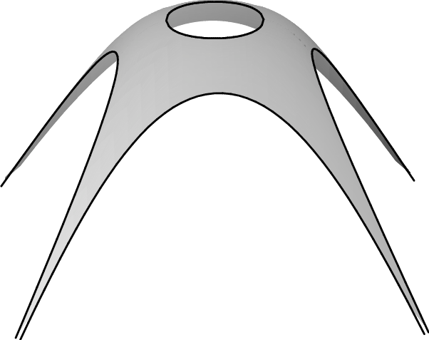

We distinguish between the unbounded complementary components and the bounded complementary components.
3.2.4 Surface tension
Theorem 2.1 gave, for a fixed magnetic field, a two-parameter family of EGMs . Let us vary the magnetic field as in Section 2.3.3. Let be the measure on dimer configurations on in the presence of an additional parallel magnetic field . We define to be the limit of as and let be its partition function per fundamental domain.
We can compute in two different ways. On the one hand, the characteristic polynomial becomes and, hence, by Theorem 3.3 we have , where is the the Ronkin function of . On the other hand, using Lemma 2.2 and basic properties of the surface tension (see Section 2.2.3) we obtain
| (5) |
In other words, is the Legendre dual of the surface tension. Since the surface tension is strictly convex, the Legendre transform is involutive and we obtain the following
Theorem 3.6.
The surface tension is the Legendre transform of the Ronkin function of the characteristic polynomial .
Recall that the Ronkin function is linear on each component of the amoeba complement. We will call the corresponding flat pieces of the graph of the Ronkin function facets. They correspond to conical singularities (commonly referred to as “cusps”) of the surface tension . The gradient of the Ronkin function maps to the Newton polygon . It is known that the slopes of the facets form a subset of the integer points inside [14]. Therefore, we have the following immediate corollary:
Corollary 3.7.
The surface tension is strictly convex and is smooth on the interior of , except at a subset of points in . Also, is a piecewise linear function on , with no slope discontinuities except at a subset of points in .
In Section 5, we will see that the spectral curves of dimer models are always very special real plane curves. As a result, their amoebas and Ronkin function have a number of additional nice properties, many of which admit a concrete probabilistic interpretation.
The following Figure 7 shows the Legendre dual of the Ronkin function from Figure 5. It is the surface tension function for certain periodically weighted dimers on the square grid with fundamental domain and also for the uniformly weighted dimers on the square-octagon graph.

4 Phases of the dimer model
4.1 Frozen, liquid, and gaseous phases
We will show that EGMs with distinctly different qualitative properties are possible in a general periodic dimer model. The different types of behavior can be classified as frozen, liquid, and gaseous. We will take the fluctuation of the height function as the basis for the classification. This, as it will turn out, is equivalent to the classification by the rate of decay of correlations.
Let and be two faces of the graph and consider the height function difference . An EGM is called a frozen phase if some of the height differences are deterministic—i.e., there exist distinct and arbitrarily far apart for which is deterministic. An example is the delta-measure on the brick-wall matching of the square grid.
A non-frozen EGM is called a gaseous phase or smooth phase if the height fluctuations have bounded variance, i.e., the variance of the random variable is bounded independently of and . A non-frozen EGM is called a liquid phase or rough phase if the -variance of the height difference is not bounded. The difference between the smooth and rough phases is illustrated in Figure 8.

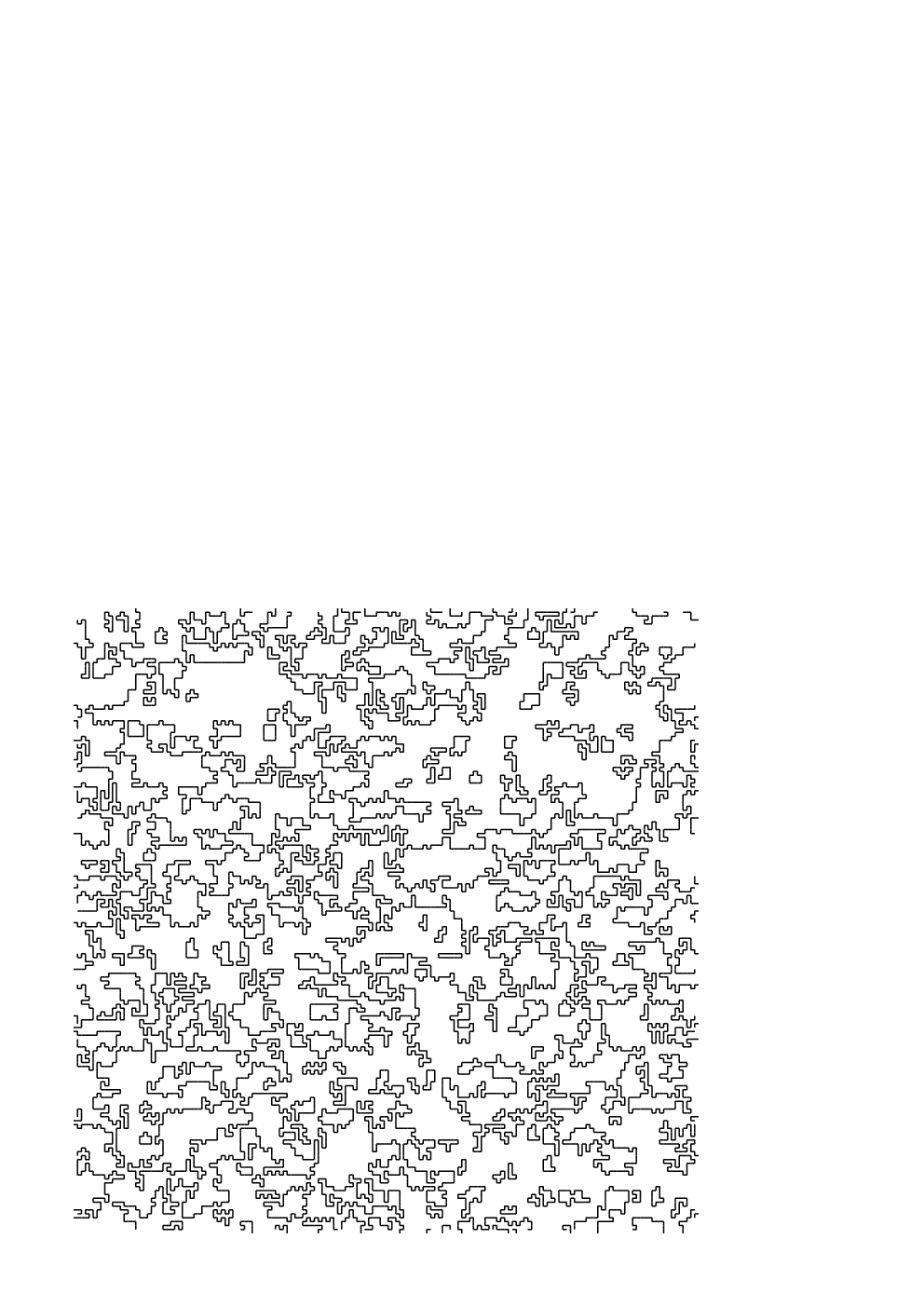
We will prove in Theorem 4.5 that in the liquid phase the variance of grows universally like times the logarithm of the distance between and . The following is our main result about phases:
Theorem 4.1.
The measure is frozen, liquid, or gaseous, respectively, when is respectively in the closure of an unbounded complementary component of , in the interior of , or in the closure of a bounded complementary component of .
This theorem is proved in the next three sections. In Corollary 9.1.2 of [18] there is a different proof that when lies in the interior of , can only be smooth if and are integers.
We will see that in the liquid and gaseous phases the edge-edge correlations decay polynomially and exponentially, respectively. In the frozen case, some edge-edge correlations do not decay at all.
4.2 Frozen phases
4.2.1 Matchings and flows
Recall the interpretation of a matching as a black-to-white unit flow. If is a matching and is the reference matching in the definition of the height function, then the difference of the flows defines a divergence-free flow. The height function of is the corresponding flux, that is, for two faces , is the amount of flow crossing any dual path from to . For two adjacent faces let be the maximal possible (oriented) flow along the edge between them (where is oriented so that is on its left). This is the forward capacity of the oriented edge . That is, if , its capacity is from its black vertex to its white vertex, and in the other direction; if , its capacity is from its white vertex to its black vertex, and zero in the reverse direction. For any two faces and let be the minimum, over all dual paths from to , of the sum of the capacities of the segments oriented to cross the path from left to right. By the max-flow-min-cut theorem, a function is the height function for a tiling if and only if
Now let . If there is no tiling with height function having slope then there is a face and such that . We claim that in this case there is a face path from to some translate on which and all faces along this path are of distinct types, that is, are not translates of each other (except for the first and last faces). To see this, note that if a face path passes through two faces of the same type, say and , then one of the two paths and will necessarily satisfy the strict inequality.
But up to translation there are only a finite number of face paths which start and end at the same face type and which pass through each face type at most once. Each such path gives one restriction on the slope: where is the translation of the path.
In particular the Newton polygon is the set of defined by the intersection of the inequalities , one for each of the above finite number of paths. If is on the edge of , the path from the corresponding inequality has maximal flow, that is, in a tiling of slope all edges on are determined: they must occur with probability or .
4.2.2 Frozen paths
When is in an unbounded component of the complement of the amoeba, we prove that is in a frozen phase.
The slope of is an integer point on the boundary of . By the argument of the previous section, there is a face path on , with homology class perpendicular to , for which every edge crossing each lift of is present with probability or for . These lifts constitute frozen paths in the dual . Edges which are in different components of the complement of the set of frozen paths are independent.
For each corner of there are two sets of frozen paths, with different asymptotic directions. The components of the complements of these paths are finite sets of edges. The edges in each set are independent of all their translates.
4.3 Edge-edge correlations
For a finite planar graph the inverse of the Kasteleyn matrix determines the edge probabilities: the probability of a set of edges being in a random matching is the determinant of the corresponding submatrix of , times the product of the edge weights [10].
For a graph on a torus the corresponding statement is more complicated: We have
Theorem 4.2 ([2]).
The probability of edges occurring is in a random matching of equals times
| (6) |
Here the determinants are minors of . The asymptotics of this expression are again complicated by the zeros of on . The entries in have the form (see [2])
where is one of a finite number of polynomials (depending on where and sit in their respective fundamental domains: is an entry of where is the matrix of Lemma 3.1) and is the translation taking the fundamental domain containing to the fundamental domain containing .
This expression is a Riemann sum for the integral
except near the zeros of . However the contribution for the root nearest to a zero of is negligible unless is at distance of the zero. But if this is the case then replacing with any at distance at least from makes the contribution for this root negligible. Thus we have
where the limit is taken along a subsequence of ’s.
Since all the have the same limit along a subsequence of s, their weighted average (as in (6)) with weights (weights which sum to one and are bounded between and ) has the same (subsequential) limit. This subsequential limit defines a Gibbs measure on . By Theorem 2.1, this measure is the unique limit of the Boltzmann measures on . Thus we have proved
Theorem 4.3.
For the limiting Gibbs measure , the probability of edges where , is
where, assuming and are in a single fundamental domain,
| (7) |
We reiterate that where is a polynomial in and .
4.4 Liquid phases (rough non-frozen phases)
4.4.1 Generic case
When is in the interior of the amoeba, either has two simple zeros on the unit torus or a real node on the unit torus (see Theorem 5.1, below). In the case of simple zeros (see Lemma 4.4 below), decays linearly but not faster, as . This implies that the edge covariances decay quadratically:
| (8) |
In section 4.4.2 we show that in the case of a real node we have similar behavior.
Lemma 4.4.
Suppose that , , and is a smooth function on with a single zero at and satisfying
Then we have the following asymptotic formula for the Fourier coefficients of :
Note that if has simple zeros, can be written as a sum of terms, each of which is of the above form.
Proof.
Replacing with and with we have
By adding a smooth function (whose Fourier coefficients decay at least quadratically) to we can replace with
The integral is therefore
We first integrate over the variable : the integrand is a meromorphic function of with a simple pole in the upper half plane if . Change the path of integration to a path from to followed by the upper half of a semicircle centered at the origin of radius . The residue theorem then yields
which gives the result. ∎
We now compute the variance in the height function.
Theorem 4.5.
Suppose that the zeros of on are simple zeros at and . Let be the derivatives of with respect to and at . Then the height variance between two faces and is
where is the linear mapping .
Since is a non-degenerate linear mapping, the above expression for the variance is equivalent to However it appears that a slightly finer analysis would improve the little-o error in the statement to , so we chose to leave the expression in the given form.
Proof.
Define . Let be four faces, all of which are far apart from each other. We shall approximate To simplify the computation we assume that and are translates of each other, as well as and . Let be a path of translates of from to , with being a single step in . Similarly let be a path from to . We assume that these paths are far apart from each other.
Then
| (9) |
We consider one element of this sum at a time. There are three cases to consider: when and are both horizontal, both vertical, and one vertical, one horizontal.
From Lemma 4.4, for large we have
Recall that the matrix satisfies . Since is a simple zero of , has co-rank . In particular must have rank . We write where
Let be the edges crossing a “positive” face path from to , that is, a face path with the property that each edge crossed has its white vertex on the left. Similarly let be the edges crossing a positive face path from to . Then
Assuming these faces are far apart, this is equal to
| (10) |
When we combine the cross terms we get an oscillating factor or its conjugate, which causes the sum (9) of these terms when we sum over and to remain small. So the leading term for fixed is
| (11) |
Now we claim that if then
and when then
and similarly for . To see this, note first that the function is a function on edges which is a closed -form, that is, a divergence-free flow. In particular the sum is independent of the choice of face path (in the same homology class). We can therefore assume that the face paths are equal to either or according to whether they are horizontal or vertical. Suppose for example and differentiate with respect to and evaluate at : we get
Applying from the right to both sides, using and , and then multiplying both sides by , this becomes
However , so we get
and since the claim follows. The same argument works for .
Recall that was the translation between the fundamental domains containing and . In the sum (9), let be the position of the fundamental domain of and that of . Let and . The sum (9) becomes (up to lower order terms)
where is the linear map This integral evaluates to
To approximate the height variance let be close to and close to (but still far enough apart on the scale of the lattice so that the above approximations hold). Then as while and are remaining bounded, the variance is
∎
4.4.2 Case of a real node
In this section we show how to modify the above proof in case has a real node. This happens when the two simple zeros merge into a single zero at one of the four points , and there. In this case the slope of the corresponding EGM is integral but the amoeba does not have a complementary component, The component is reduced to a point (and is therefore not “complementary”).
The canonical example of this behavior is the square grid with uniform weights and a fundamental domain; in this case , and there is a real node at .
Since is a continuous function of the edge weights, so is the variance of the height between two points. When has a node, at say , the polynomial has two simple zeros on as long as are sufficiently close to but not equal to . So the height variance of is the limit of the height variances of as .
In fact suppose without loss of generality that the node is at and has the expansion
where and denotes terms of order at least . Then near the node a point on satisfies either or where , which are necessarily non-real, are the roots of .
The proof of Theorem 4.5 is valid for except for one assertion, where we ignored the cross terms in equation (11). Indeed, when are each close to the cross terms do not oscillate. However we will show that as tends to the node. Along with the complex conjugate equation this proves that the cross terms make no contribution.
The cross terms of (11) give
| (12) |
where recall that are tending to at the node. We first show that and similarly for its complex conjugate. Recall the equation . Differentiating with respect to we find
At a point on we have and at we have . Applying to the right and evaluating in the limit as tends to the node, we have
so that at the node. Since can be chosen polynomial in the quantity necessarily vanishes to order at least one at the node (as do and ).
Let be the limit at the node of when and the same limit when , so we may write
at the node. The cross terms are then
A short computation now shows that, since , this is not a closed -form in or unless .
However since the height function differences do not depend on the path , the cross terms should necessarily be a closed -form. So . We have proved
Theorem 4.6.
Suppose has a real node on the unit torus, and
Then the height variance between two faces and is
where is the linear mapping , being the root of .
4.5 Gaseous phases (smooth non-frozen phases)
When is in a bounded complementary component, has no zeros on the unit torus. As a consequence decays exponentially fast in .
Proposition 4.7.
The height variance is bounded.
Proof.
The height difference can be measured along any path from to . Suppose a dual path from to is chosen so that each edge crosses an edge of with black vertex on its left. Then the height difference is a constant plus the sum of the indicator functions of the edges on the path: . Suppose we have two such paths , consisting of edges and respectively, which are close only near their endpoints. The height variance is then the sum of the covariances of and :
However these covariances are exponentially small except when both and are near the endpoints or . In particular the above summation is a geometric series, which has sum bounded independently of the distance between and . ∎
4.6 Loops surrounding the origin
Smooth phases are characterized by their bounded height variance or exponential decay of correlation. Here is another characterization of smooth phases in terms of loops in the union of two perfect matchings sampled independently.
Theorem 4.8.
A non-frozen EGM is smooth if and only if when two perfect matchings and are chosen independently from , there are almost surely only finitely many cycles in that surround the origin. Similarly, a non-frozen EGM is rough if and only if when two perfect matchings and are chosen independently from , there are almost surely infinitely many cycles in that surround the origin.
Proof.
Since having infinitely many cycles surround the origin is a translation-invariant event, it is clear that if is an EGM, then there are either -almost-surely infinitely many cycles or -almost-surely finitely many cycles surrounding the origin. If the former is the case, it is easy to see that the variance is unbounded; to see this, simply use the fact that, conditioned on the positions of the cycles, the two orientations of a given cycle (i.e., which alternative set of edges in the cycle belongs to which of the ) are equally likely, and orientations of the cycles are independent of one another. (Note that the orientation of the cycle determines whether the height difference of the two height functions goes up or down when we cross that cycle.)
Now suppose that there are almost surely only finitely many cycles surrounding the origin. Lemma 8.4.3 of [18] further implies that if two perfect matchings and are sampled independently from , then the union almost surely contains no infinite paths. It follows that the height difference between the two height functions is constant on the infinite cluster of faces that are not enclosed in any loops. Lemma 8.3.4 of [18] then implies that is smooth with respect to the (differently formulated but actually equivalent) definition given in Chapter 8 of [18], and Lemmas 8.1.1 and 8.1.2 imply that the height difference variances remain bounded in this case. ∎
5 Maximality of spectral curves
5.1 Harnack curves
The characteristic polynomial has real coefficients and, hence, the spectral curve is a real plane curve (in fact, it is more natural to consider the spectral curve as embedded in the toric surface corresponding to the Newton polygon of ). While all smooth complex curves of given genus are topologically the same, the number and the configuration of the ovals of a real plane curve can be very different. In particular, there is a distinguished class of real plane curves, known as Harnack or maximal curves, which have the maximal number of ovals (for given Newton polygon) in the, so to speak, best possible position. The precise topological definition of a Harnack curve can be found in [14]; here we will use the following alternative characterization of a Harnack curve obtained in [15]. Namely, a curve is Harnack if and only if the map from the curve to its amoeba is -to- over the amoeba interior (except for a finite number of real nodes where it is -to-). The main result of this section is the following
Theorem 5.1.
For any choice of nonnegative edge weights the spectral curve is a Harnack curve.
5.2 Proof of maximality
Maximality is an important property and several proofs of it are available. In many respects, it resembles the notion of total positivity [4, 7] and the proof given below exploits this analogy. Proofs of maximality based on different ideas can be found in [12, 13].
First observe that by the -to- property, being Harnack is a closed condition, hence it is enough to prove that spectral curve is Harnack for a generic choice of weights. Furthermore, it is easy to see that we can obtain any periodic planar bipartite graph as a limit case of the periodically weighted hexagonal lattice when some of the edge weights are zero. It is therefore, enough to consider the case of generic periodic weights on the hexagonal lattice with fundamental domain.
-2,0)(12,10)
By definition, is a determinant of an matrix whose rows and columns are indexed by the white and black vertices in the fundamental domain. We can also write as a determinant of an matrix using transfer matrices as follows. The equation means that there exists a nonzero function on black vertices annihilated by the operator . We can construct such a function row by row as follows: given the values of on a horizontal row of black vertices as in Figure 9, the equation determines the values of on the row below it. The corresponding linear map is given by , where is the transfer matrix of the form
| (13) |
Iterating this procedure once around the period, we get a consistency relation, which gives
Suppose now that for some point the torus contains more than 2 points of the curve . By changing the magnetic field, we can assume that . That is, we can assume that for a pair of points and on the spectral curve we have
Since being not Harnack is an open condition, we can find a nearby curve for which both and are roots of unity. It is easy to see (a more general statement is proved in [12]) that we can achieve this by a small perturbation of the dimer weights. So, we can assume that for some integer .
Taking as the new horizontal period, we find that the matrix
| (14) |
has more than 2 eigenvalues of the same absolute value. We will now show that this is impossible.
This follows from the following lemma which is a version of a standard argument in the theory of total positivity (cf. [4]).
Lemma 5.2.
Suppose that all odd-size minors of a matrix are nonnegative and that there exists such that all odd-size minors of are positive. Then the eigenvalues of have the following form
Remark, in particular, that if then both of these eigenvalues are real.
Proof.
Let us order the eigenvalues of so that
Since all matrix elements of are nonnegative and all matrix elements of are positive, the Perron-Frobenius theorem implies that is simple, positive, and that
Now consider the action of the matrix in the third exterior power of the original space . The matrix elements of this action are the minors of and, hence, Perron-Frobenius theorem again applies. The eigenvalues of this action are the numbers
It follows that the number is real, positive, and greater in absolute value than for any . It follows that
Iteration of this argument concludes the proof. ∎
It is immediate to see that any matrix of the form satisfies the hypothesis of the lemma. Matrices with nonnegative minors of any given order form a semigroup, so all odd-size minors of (14) are nonnegative. Genericity implies that all odd-size minors of are positive for some large enough . This concludes the proof.
5.3 Implications of maximality
5.3.1 Phase diagram of a dimer model
The -to- property immediately implies that:
- (i)
the only singularities of the amoeba map are folds over the boundary of the amoeba;
- (ii)
the boundary of the amoeba is the image of the real locus of the spectral curve;
- (iii)
to any lattice point in the interior of the Newton polygon corresponds either a bounded component of the amoeba complement or an isolated real node of the spectral curve. In particular, the number of holes in the amoeba equals the geometric genus of the curve.
For a general plane curve, more complicated singularities of the amoeba map are possible, which are then reflected in more complicated singularities of the Ronkin function and, hence, of its Legendre dual. In fact, we have used the -to- property in Section 4 in the classification of the phases of the dimer model. In this sense, the probabilistic meaning of maximality is the absence of any exotic phases with anomalous decay of correlations.
Part (iii) implies that the gaseous phases persist unless the corresponding component of the amoeba complement shrinks to a point and a nodal singularity develops. In particular, generically, the spectral curve is smooth and all gaseous phases are present. Conversely, if no gaseous phases are present then the spectral curve has the maximal possible number of nodes and hence is a curve of genus zero. It is shown in [12] that the latter case corresponds to isoradial dimers studied in [11]. It is also shown in [12] that all Harnack curves arise as spectral curves of some dimer model.
To summarize, part (iii) implies the following:
Theorem 5.3.
The number of gaseous phases of a dimer model equals the genus of the spectral curve. For a generic choice of weights, the dimer model has a gaseous phase for every lattice point in the interior of the Newton polygon and a frozen phase for every lattice point on the boundary of .
Part (ii) shows that the phase boundaries can be easily determined. In fact, the amoeba of a Harnack curve can be defined by a single inequality
| (15) |
where the product is over all 4 choices of signs. Indeed, it is clear that the product in (15) changes sign whenever we cross the amoeba boundary and, generically, is positive when or are large. We remark that for a general, non-Harnack, curve it is a rather nontrivial task to determine its amoeba.
Using the interpretation of as the expectation of with respect to the measure , see Section 3.1.3, we arrive at the following:
Theorem 5.4.
The minimal free energy measure is smooth (that is, frozen or gaseous) if and only if the -measure of one of the four classes of matchings of exceeds , or can be made more than by an arbitrarily small perturbation of the dimer weights.
5.3.2 Universality of height fluctuations
In Theorem 4.5 we proved that in a liquid phase the variance of the height function difference grows like times the logarithm of the distance. The proof of that theorem shows that the constant in front of the logarithm is directly connected to the number of roots of the characteristic polynomial on the unit torus. In particular, maximality was used in the essential way to show that this constant is always . In fact, the universality of this constant is equivalent to maximality.
5.3.3 Monge-Ampère equation for surface tension
It follows from the results of [15] that the Ronkin function of a Harnack curve satisfies the following Monge-Ampère equation
| (16) |
for any in the interior of the amoeba. By the well-known duality for the Monge-Ampère equation, this implies the analogous equation for the surface tension function.
Theorem 5.5.
We have
| (17) |
It should be pointed out that in [6] it was argued that for certain class of random surface models the equation (17) should be satisfied at any cusp of the surface tension. It seems remarkable that in our case (17) is satisfies not just at a cusp but identically. For a general random surface model, we only expect the left-hand side of (17) to be positive, by strict concavity.
The geometric meaning of the equations (16) and (17) is that the gradients of and , which are mutually inverse maps, are area-preserving, up to a factor. This leads to another characterization of Harnack curves as curves with amoebas of maximal possible area for given Newton polygon , namely times the area of . It would be interesting to find a probabilistic interpretation of this.
5.3.4 Slopes and arguments
Recall that by the results of Section 3.2.4 the slope of the Ronkin function at a point equals the slope of the measure . Suppose that the point is in the interior of the amoeba and let be one of its two preimages in the spectral curve. Maximality connects the slope with the arguments and as follows.
Theorem 5.6.
We have
Proof.
We have
| (18) |
The inner integral counts, for fixed, the number of zeros of inside . As varies over the unit circle the number of zeros is locally constant with unit jumps whenever a zero crosses the circle. These jump points are precisely the points where has a root on , that is precisely the two points and where and its conjugate are the unique zeros of on . ∎
6 Random surfaces and crystal facets
The goal of this section is to review some known facts about random surfaces in order to say precisely what Theorem 3.6 and Theorem 4.1 imply about crystal facets and random surfaces based on perfect matchings. We begin with some analytical results.
6.1 Continuous surface tension minimizers
A standard problem of variational calculus is the following: given a bounded open domain and any strictly convex surface tension function , find the function whose (distributional) gradient minimizes the surface tension integral
subject to the boundary condition that extends continuously to a function on the boundary of and the volume condition that
for some constant . In our setting, we may also assume that whenever lies outside of the closure of the Newton polygon , so that is necessarily Lipschitz. The following result is well known (see [2], [18] for details and references).
Proposition 6.1.
If there exists any , satisfying prescribed volume and boundary constraints and satisfying , then the surface tension minimizer is unique and its gradient is almost everywhere defined.
Both and are functions from to . The Euler-Lagrange equation for the functional takes the following form:
Proposition 6.2.
Let be the surface tension minimizer described above. Then whenever , is at , and is smooth at , we have:
| (19) |
for some constant , which depends on and . If is also the minimal surface tension function when the volume constraint is ignored, then (19) holds with .
The archetypal solution to the equation in Lemma 6.2 is the Legendre dual of , which, in our setting, is the Ronkin function . By construction
throughout the amoeba—in particular, the divergence is constant. By analogy with the case of the Ronkin function we say that has a facet of slope if is equal to on some open subset of .
If is linear of any slope on the boundary of , then it is easy to see that the minimal surface tension function, ignoring the volume constraint, is linear of slope , has (trivially) a facet of slope , and satisfies (19) with . If we require, however, that , so that the volume constraint exerts some non-zero amount of pressure (upward or downward) on the surface, then Lemma 6.2 and Theorem 3.7 imply that the slope of any facet of must be a lattice point inside . In other words, the facet slopes of the Ronkin function represent all possible facet slopes of the dimer model.
6.2 Concentration inequalities for discrete random surfaces
In this section, we aim to show that the surface tension minimizing shapes and facets described in Section 6.1 are approximated by perfect-matching-based discrete random surfaces. First, suppose that is a domain in , that is continuous Lipschitz function defined on , and that is a surface tension minimizer (with no volume constraint) which agrees with on the boundary.
Next, denote by the infinite graph whose embedding into has been re-scaled by a factor of . For example, when , then is a grid mesh that is times finer than . Suppose that is a sequence of simply connected subgraphs of that approximate from the inside in the sense that
- 1.
The embedding of is contained in for all .
- 2.
The Hausdorff distance between the boundary of and the boundary of tends to zero in .
- 3.
Each admits at least one perfect matching, and for these matchings, the height functions on the boundary of are such that tends to zero in (where is treated as a function on a subset of the points in , by letting denote the height at the face of containing ).
For each , define to be the Boltzmann measure on perfect matchings of . Intuitively, we would expect that for sufficiently large values of , the normalized function will closely approximate the continuous function with high probability. A version of this statement is proved in [2] in the case . Analogous but more general statements (in the form of large deviations principles) are discussed in Chapter 7 of [18] (see the paragraphs on Lipschitz potentials in Sections 7.3 through 7.5). In both [2] and [18], the results imply that, for a fixed value of , tends to zero exponentially in . Also, if is a point at which , we would expect the local statistics of , near the point , to be those of the Gibbs measure . More precise versions of this statement can be found in Chapter 7 [18]. The issue of weighting by enclosed volume is addressed briefly in Section 7.5 of [18].
References
- [1] R. Cerf and R. Kenyon, The low-temperature expansion of the Wulff crystal in the three-dimensional Ising model, Comm. Math. Phys 222 (2001),147-179.
- [2] H. Cohn, R. Kenyon, J. Propp, A variational principle for domino tilings, J. Amer. Math. Soc., 14 (2001), no.2, 297-346.
- [3] J. C. Fournier, Pavage des figures planes sans trous par des dominos: fondement graphique de l’algorithme de Thurston et parallélisation. C. R. Acad. Sci. Paris Sér. I Math. 320 (1995), no. 1, 107–112.
- [4] F. Gantmacher and M. Krein, Oscillation matrices and kernels and small vibrations of mechanical systems, AMS Chelsea Publishing, 2002.
- [5] I. M. Gelfand, M. M. Kapranov, A. V. Zelevinsky, Discriminants, resultants, and multidimensional determinants, Mathematics: Theory & Applications. Birkäuser Boston, Inc., Boston, 1994.
- [6] P. Ferrari, M. Praehofer, H. Spohn, Fluctuations of an Atomic Ledge Bordering a Crystalline Facet, cond-mat/0303162.
- [7] S. Karlin, Total positivity, Stanford University Press, 1968.
- [8] P. Kasteleyn, Graph theory and crystal physics, 1967 Graph Theory and Theoretical Physics pp. 43–110 Academic Press, London
- [9] R. Kenyon, An introduction to the dimer model, math.CO/0310326.
- [10] R. Kenyon, Local statistics of lattice dimers, Ann. Inst. H. Poincaré, Probabilités 33(1997), 591–618.
- [11] R. Kenyon, The Laplacian and operators on critical planar graphs Invent. Math. 150 (2002), 409-439.
- [12] R. Kenyon and A. Okounkov, Dimers and Harnack curves, preprint.
- [13] R. Kenyon and S. Sheffield, Dimers, Tilings and Trees, math.CO/0310195.
- [14] G. Mikhalkin, Amoebas of algebraic varieties, math.AG/0108225.
- [15] G. Mikhalkin and H. Rullgård, Amoebas of maximal area, Internat. Math. Res. Notices 2001, no. 9, 441–451.
- [16] A. Okounkov, N. Reshetikhin, C. Vafa, Quantum Calabi-Yau and Classical Crystals, hep-th/0309208.
- [17] P. Pieranski, P. Sotta, D. Rohe, M. Imperor-Clerc, Devil’s Staircase–Type Faceting of a Cubic Lyotropic Liquid Crystal, Phys. Rev. Lett. 84, 2409 (2000).
- [18] S. Sheffield, PhD Thesis, Standford Univ. 2003.
- [19] G. Tesler, Matchings in graphs on non-orientable surfaces. J. Combin. Theory Ser. B 78 (2000), no. 2, 198–231.
- [20] W. P. Thurston, Conway’s tiling groups Amer. Math. Monthly 97 (1990), no. 8, 757–773.