Energy Flow from Open to Closed Strings in a Toy Model of Rolling Tachyon
Abstract
We study the toy model of interacting open and closed string tachyons which demonstrates some interesting properties of the unstable D-brane decay scenario. We compute a stress tensor of the system and study the energy and pressure dynamics. We show that the total energy of the system is conserved. We separate the stress tensor into two parts corresponding to open and closed strings and study the energy flow from open to closed strings. The two vacua of the system could be interpreted as corresponding to the unstable D-brane background and the open string tachyon vacuum. We study how for spatially homogenous solution interpolating between these two vacua the total energy of the open string dissipates to the closed string.
pacs
11.25.-wI Introduction
Physical process of the unstable D-brane decay has recently attracted a lot of attention 0203211; 0207107; Kluson; 0209122; Yang; VolYa; AJ; 0303139; 0304163; 0304213; 0305011; 0305159; 0305191; VSVYaV; Oh. This process has been investigated in frameworks of boundary CFT 0203211; 0303139 and within open string field theory (OSFT) 0207107; Kluson; AJ; 0304213. To work within OSFT a level-truncated scheme has been usually employed. Dynamical equations in this approach are rather interesting from mathematical point of view since they contain an infinite number of derivatives. These equations could be represented in the integral form that corresponds to a nonlocal interaction found in string theories. For detailed analysis of such types of equations see for example BFOW; 0207107; Yang; VolYa; AJ, for some rigorous mathematical results in this field see VSVYaV. Despite of these mathematical difficulties several interesting results where obtained. In particular special time dependent solutions of classical equations of motion where constructed in p-adic string theory VVZ; Kh; Fr-rev in papers BFOW; 0207107 and in SSFT in papers VolYa; AJ. These solutions describe the tachyon field which starts from the unstable vacuum of the system with non-zero velocity and tends to the stable one reaching it at infinite time. The D-brane’s tension at the unstable vacuum is expected to be at its maximum and vanishing while moving to the stable one.
An interesting point in the current development of the unstable D-brane decay is the disagreement between the conformal field theory considerations and the results obtained in the level-truncated open cubic string field theory approximations. This gave rise to an investigation of open-closed interacting string models where it was proposed that one has to take into account the fact that the D-brane’s energy dissipates to the closed string while reaching the resulting stable vacuum.
In this paper we consider a model with two interacting tachyon fields recently proposed in Oh. The model could be seen as a simplification of level-truncated Open-Closed String Field Theory (OCSFT) where several terms are omitted even on the first nontrivial level. Although this model could be considered only as a simplified model of OCSFT it has a time dependent solution interpolating between two vacua of the system. This solution starts from the first vacuum interpreted as an unstable D-brane background and tends to the second one where the D-brane disappears Oh. Here we show that for this solution the conserved energy dissipates from the open string tachyon to the closed one. This coincides with the expected behavior of the D-brane’s energy.
The paper is organized as follows. In Section II we describe the model and study its dependance on the parameters. Then in Section III we compute a stress tensor of the model and separate the terms corresponding to open and closed tachyons. Finally in Section IV we study energy and pressure dynamics. First, we provide a direct prove of the energy convergence. Then using the separation of terms in the stress tensor we study energy flow from open to closed strings. We show how the energy of open string dissipates to closed one. At last we show a picture of the pressure dynamics. The pressure is negative and vanishes at infinite time.
II The Toy Model for Open and Closed String Tachyons
We study a toy model of open-closed string tachyons recently proposed in Oh. In the units with the corresponding action takes the form
| (1) |
where and are interpreted as open and closed string tachyon fields respectively Oh, and one defines
| (2a) | |||
| (2b) |
with the differential operator is understood as a series expansion
| (3) |
(about an appearance of nonlocal terms in SFT see reviews 0102085; 0111208; 0301094) and is a constant which is discussed below. The space-time is flat with the metric , so that the D’Alamber operator takes the form . The equations of motion corresponding to the action (1) are the following
| (4a) | |||
| (4b) |
Let us consider spatially homogeneous configurations. In this case the equations of motion (4a)-(4b) take the following form
| (5a) | |||
| (5b) |
where the time derivative is denoted by and , .
Equations of motion (5a)-(5b) contain a pseudo-differential operator of the form , it is defined as
| (6) |
where is a Gaussian kernel given by
| (7) |
The integral operator (6) is well defined for , see BFOW; 0207107; VolYa; VSVYaV for detailed analysis of equations with such operators.
The equations of motion have tree vacua solutions which could be easily found by the following procedure. First we solves the equation (4b) for constant , with respect to . This gives . Now substituting it to (4a) and using the fact that the fields are constant we get an equation which has three solutions
these are the vacua of the system in terms of .
The potential of the system has the form
| (8) |
Now we want to fix a constant in such a way that there are two distinct vacua with the same energy, i.e. we solve equations , with respect to and check that for this value of . The first step gives us the following values of
Although only for the values and there are two distinct vacua with the same energy.


In Oh a space homogeneous configuration was constructed numerically for the case using the following iterative procedure
| (9) |
where and the initial configuration is taken as , , where is a step function being for and otherwise. The operator could be presented in the fully integral form by differentiating the kernel (7)
| (10) |
The results of the iterative procedure (9) are presented on Fig.2.
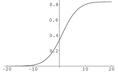

In order to support this numerical results let us study the equations (5a)-(5b) neglecting high order derivatives. This reduces the original equations to the following system (see (2a)-(2b))
| (11a) | |||
| (11b) |
Equations (11a)-(11b) could be seen as describing a mechanical system with the following potential
| (12) |
We will call potential obtained in such a way an effective mechanical potential. Note that
| (13) |
this reflects the fact that interacting terms contain second order derivatives and thus contribute to the kinetic term. We have this effect of potential-flipping only if and (we have this in our model since ), i.e. the effective “masses” are positive.
The described construction of an effective mechanical potential provide good intuition about the existence of rolling-type solutions. Indeed the shape of (Fig.1) points (at least for the case ) to the existence of kink-type solutions for the reduced system (11a)-(11b) and this usually a good sign for the original nonlocal system to have a rolling-type solution AJ; VolYa. The direct proof of existence of rolling-type solutions for our system might be rather nontrivial. Indeed the properties of the integral kernel (10) does not allow us to use the same approach as was used in VSVYaV.
Although the iterative procedure (9) demonstrates a good numerical convergence for it rapidly diverges for where the initial functions where taken to be “stepping” between the corresponding vacua
| (14) |
It is left unclear whether kink-type solution exists even for the reduced system (11a)-(11b) for this value of . Our numerical investigations show that the arch at the bottom of the potential for this case (see Fig.1, part right) prevents the trajectory started from one endpoint (14) to reach the second.
III Stress Tensor
Let us compute a stress tensor for the model and present it in the form with the separated terms corresponding to open and closed string.
We use the definition of a stress tensor from general relativity
| (15) |
We make the action (1) invariant under space-time transformations by including metric in the action
| (16) |
where the D’Alamber operator is covariant
While performing a variation of the action (16) according to (15) we will have to deal with the following expressions
| (17) |
and
| (18) |
here and below the index denotes derivation with respect to .
Let us now consider these expressions in more detail Yang; AJ. Using the following equality
we compute
| (19) |
Now for the expression (17) we obtain
| (20) |
Now let us consider the expression (18). First let us rewrite it in the following form
Using (19) and the equality Yang
we obtain
| (21) |
Now using (20) and (21) we are able to compute the stress tensor of the system
| (22) |
where the part corresponding to the open string tachyon is
and the part corresponding to the closed string tachyon is given by
where we used the equations of motion. We see that the terms of the stress tensor corresponding to open and closed strings are separated. This allows us to study the energy flow from open to closed strings.
IV Energy and Pressure Dynamics
The energy of the system is defined in terms of the stress tensor (22)
| (23) |
As it was shown in the previous section it is possible to separate the terms of the stress tensor corresponding to open and closed strings. Thus the energy of the system (23) could also be written as a sum of energies of open and closed strings.
For spatially homogeneous configurations the energy takes the form
| (24) |
where the term corresponding to open string is given by
and the term corresponding to closed string is
here and below .

One can immediately see that this energy conserves
using the identity AJ
| (25) |
we get
or simplifying
now using the equation of motion (4b) we get
We see that the time derivative of the energy is zero on the equations of motion and thus the total energy is conserved. We also see that on infinities the energy is zero and thus or at all times. The energy flow from open to closed string for the solution described in the section II is presented on Fig.3. We see that the energy contained in the open string tachyon dissipates to the closed string tachyon that could be interpreted as a transformation of the unstable D-brane’s energy to the energy of closed string Oh.
Let us now investigate the pressure of the system 0207107; Yang; AJ. The pressure is defined in terms of the stress tensor as
| (26) |

Since we consider spatially homogeneous configurations we will omit the vector index . The pressure dynamics is given by
| (27) |
The pressure dynamics is presented on Fig.4. Since the total energy is zero and the fields are constant at infinities we see from (27) that the pressure vanishes as . The pressure contains two positive terms with only second-order derivatives of and and two negative terms with high-order derivatives of and . These terms are presented separately on Fig.5. We see that there is a nontrivial compensation of the positive terms making the total pressure being negative.

Let us note that the form (27) is rather nontrivial from computational point of view. In particular we where able to present the last two terms in such a way that the first exponent is well defined in terms of the integral operator (6) for all while there is no such possibility for the second exponent in both terms – the Gaussian kernel diverges at . Although for near to we where able to use the series expansion (3) without loss of precision.
V Conclusion
In this paper a simplified model of the unstable D-brane decay in the open-closed string field theory was studied. We have computed a stress tensor of the system and presented it as a sum of two terms corresponding to open and closed strings. We have obtained the energy of the system and proved its convergence. The separation of energies of open and closed strings allowed us to study the energy flow from open to closed strings. We have considered a time-dependant solution interpolating between two vacua of the system for the case . We have showed that the energy of open string dissipates to the closed string. The question of existence of such interpolating solution for the case is left open. The next important step would be to generalize these results to the full level-truncated OCSFT and study the D-brane’s decay there.
Acknowledgements.
The authors are grateful to I.Ya. Aref’eva for attention and discussions. L.J. was financially supported by the grant RFBR-02-01-00695 and by Dynasty Foundation and International Center for Fundamental Physics in Moscow, Ya.V. was financially supported by the grants RFBR-02-01-01084 and RFBR-MAS-03-01-06466. All numerical computations in this work where performed using a C++ library developed by the authors, for visualization we have used the Mathematica system.References
- (1) A. Sen, Rolling Tachyon, JHEP 0204, 048 (2002), hep-th/0203211; A. Sen, Tachyon Matter, JHEP 0207, 065 (2002), hep-th/0203265; A. Sen, Field Theory of Tachyon Matter, Mod. Phys. Lett. A 17, 1797-1804 (2002), hep-th/0204143. A. Sen, Time evolution in open string theory, JHEP 0210, 003 (2002), hep-th/0207105.
- (2) N. Moeller and B. Zwiebach, Dynamics with infinitely many time derivatives and rolling tachyons, JHEP 0210, 034 (2002), hep-th/0207107.
- (3) J. Kluson, Time Dependent Solution in Open Bosonic String Field Theory, hep-th/0208028.
- (4) A. Sen, Time and tachyon, hep-th/0209122.
- (5) H. Yang, Stress tensors in p-adic string theory and truncated OSFT, JHEP 0211, 007 (2002), hep-th/0209197.
- (6) Yaroslav Volovich, Numerical Study of Nonlinear Equations with Infinite Number of Derivatives, J. Phys. A: Math. Gen. 36 (2003) 8685-8701, math-ph/0301028.
- (7) I.Ya. Aref’eva, L.V. Joukovskaya and A.S. Koshelev, Time Evolution in Superstring Field Theory on non-BPS brane. I. Rolling Tachyon and Energy-Momentum Conservation, JHEP 0309 (2003) 012, hep-th/0301137; I.Ya. Aref’eva, Rolling Tachyon in NSSFT, 35-th Ahrenshoop meeting, Fortschr. Phys., 51 (2003) 652; I.Ya. Aref’eva and L.V. Joukovskaya, Rolling Tachyon on non-BPS brane, Lectures given at the II Summer School in Modern Mathematical Physics, Kopaonik, Serbia, 1-12 Sept. 2002.
- (8) N. Lambert, H. Liu, J. Maldacena, Closed strings from decaying D-branes, hep-th/0303139.
- (9) M. Fujita, H. Hata, Time Dependent Solution in Cubic String Field Theory, JHEP 0305, 043 (2003), hep-th/0304163.
- (10) N. Moeller, M. Schnabl, Tachyon condensation in open-closed p-adic string theory, hep-th/0304213.
- (11)
A. Sen, Open and Closed Strings from Unstable D-branes,
hep-th/0305011. - (12) I.R. Klebanov, J. Maldacena, N. Seiberg, D-brane Decay in Two-Dimensional String Theory, JHEP 0307, 045 (2003), hep-th/0305159.
- (13) Y. Demasure, R.A. Janik, Backreaction and the rolling tachyon – an effective action point of view, hep-th/0305191.
- (14) V.S. Vladimirov, Ya.I. Volovich, Nonlinear Dynamics Equation in p-adic String Theory, Theor. Math. Phys., Vol.138, No.3, pp.297-309, (2004), math-ph/0306018.
- (15) K. Ohmori, Toward Open-Closed String Theoretical Description of Rolling Tachyon, Phys.Rev. D69 (2004) 026008, hep-th/0306096.
- (16) L. Brekke, P.G.O. Freund, M. Olson, E. Witten, Non-archimedian string dynamics, Nucl.Phys. B302 (1988) 365.
- (17) K. Ohmori, A Review on Tachyon Condensation in Open String Field Theories, hep-th/0102085.
- (18) I.Y. Arefeva, et al., Noncommutative field theories and (super)string field theories. In Campos do Jordao 2001, Particles and fields 1-163, hep-th/ 0111208
- (19) W. Taylor, Lectures on D-branes, tachyon condensation and string field theory, hep-th/0301094.
- (20) V.S. Vladimirov, I.V. Volovich, E.I. Zelenov, p-adic Analisis and Mathematical Physics, WSP, Singapore, 1994.
- (21) A.Yu. Khrennikov, -adic valued distributions in mathematical physics, Kluwer Acad. Publ., Dordrecht, 1994.
- (22) L. Brekke and P.G. Freund, P-Adic Numbers in Physics, Phys.Rept. 233, 1 (1993)