跳到论文正文
W Papers独立论文阅读器 arXiv:math-ph/0308005 论文正文 计算阅读时间 · 0%
引用这篇论文根据当前论文元数据生成,正式投稿前建议核对。


License: Assumed arXiv.org perpetual non-exclusive license
arXiv:math-ph/0308005v1 [math-ph] 05 Aug 2003

No Quantum Ergodicity for Star Graphs

G. Berkolaiko    J.P. Keating    B. Winn    Department of Mathematics, University of Strathclyde, Glasgow G1 1XH, UK.    School of Mathematics, University of Bristol, Bristol BS8 1TW, UK.
25th25^{\rm th} July, 2003
Abstract

We investigate statistical properties of the eigenfunctions of the Schrödinger operator on families of star graphs with incommensurate bond lengths. We show that these eigenfunctions are not quantum ergodic in the limit as the number of bonds tends to infinity by finding an observable for which the quantum matrix elements do not converge to the classical average. We further show that for a given fixed graph there are subsequences of eigenfunctions which localise on pairs of bonds. We describe how to construct such subsequences explicitly. These constructions are analogous to scars on short unstable periodic orbits.

1 Introduction

Let ψn\psi_{n} denote the wave-function corresponding to the nthn^{\rm th} energy level of a quantum system that has a Hamiltonian dynamical system as its classical limit. We are interested in these wave-functions in the n→∞n\to\infty limit, which corresponds to the semi-classical regime. Numerical and some theoretical evidence supports the hypothesis that their behaviour in this limit is determined by general properties of the underlying Hamiltonian such as, for example, time-reversibility, integrability and statistical properties of the flow (ergodicity, mixing, etc.). A deeper understanding of this is one of the goals of current research in quantum chaology.

When the classical Hamiltonian generates chaotic motion, the semi-classical eigenfunction hypothesis asserts that the wave-functions should equidistribute over the appropriate energy shell [Be1, V]. A physical explanation for this is that in the semi-classical limit the quantum system should mimic the behaviour of the classical system; if the classical motion is chaotic, then a typical trajectory ergodically explores the surface of constant energy in phase space. Another interpretation is that eigenstates are invariant under time evolution, so it is natural to associate them in the semi-classical limit with classical invariant sets. One such invariant set is the energy shell itself.

The Schnirelman theorem [S, CdV, Z, GL] states that for systems in which the Hamiltonian flow is ergodic the sequence of measures induced by ψn\psi_{n} converges to Liouville measure in the limit as n→∞n\to\infty along a subsequence of density one. This behaviour has been termed “quantum ergodicity”. Quantum ergodicity implies a weak version of the semi-classical eigenfunction hypothesis [BSS].

It is possible that quantum ergodic systems have subsequences of states for which the corresponding measures do not converge to Liouville measure (of course such subsequences have density zero). These subsequences, if they exist, are expected to be associated with other classical invariant sets, such as periodic orbits. The case where the limit of an exceptional subseqence is a singular measure supported on one-or-more isolated, unstable periodic orbits of the classical system is called “scarring”.

Scarred eigenstates were observed numerically by Heller [H], who proposed the first theoretical explanation for their existence, based on the semi-classical evolution of a wave-packet centred on a periodic orbit under linearised dynamics. Another important development was an understanding of the contribution to wave-functions from all periodic orbits [Bo, Be2] resulting in formulæ related to the semiclassical trace formula for the density of states. Later, the theory was extended to include non-linear effects [KH] and, more recently, situations where the orbit in question undergoes a bifurcation [KP]. A review of related works was given in [K1]. All of the above mentioned theories relate to scar effects in averages over a semiclassically increasing number of states. This may be thought of as a weakened form of scarring, because it is not clear that any one state in the averaging range causes the scar; the scars may be a collective effect. It is a much harder problem to show that a particular sequence of individual states is scarred. Currently, the only systems known rigorously to support scarring in this strong form are the cat maps [FNdB] which have non-generic spectral statistics caused by number-theoretical symmetries [Ke].

For quantum graphs [KS1] the wave-functions are the eigenfunctions of the (continuous) Laplace operator on the bonds with matching conditions at the vertices chosen to make the problem self-adjoint. There is evidence to suggest that the spectral statistics of large quantum graphs coincide with those of generic quantised, classically chaotic, systems [KS2, BSW1, BSW2, B] subject to mild conditions on the connectivity [T]. Although the classical dynamics on a graph are not Hamiltonian, they are ergodic and it might be expected that an analogue of the Schnirelman theorem should hold.

Graphs are a rich source of problems in quantum chaology and related fields. Recent works have considered: scattering problems [KS3, TM, KS4], the spacing distribution of eigenvalues [BG], nodal domain statistics [GSW], the Dirac operator on graphs [BH1, BH2], Brownian motion on graphs [CDM, D] and the important question of how to construct families of graphs with increasing numbers of bonds [PTZ].

Recently, authors have begun to investigate the wave-functions of quantum graphs. Kaplan [K2] studied eigenfunction statistics for ring-graphs using a combination of numerical techniques and analytical calculations of the short-time semiclassical behaviour of a wave-packet close to a 1-bond periodic orbit. The inverse participation ratio (a measure of localisation in a given state) was found to be well-described by this contribution, and shows deviation from the ergodically expected behaviour. Similar deviations were noticed for lattice-graphs. Remarkably, Schanz and Kottos [SK] observed that it would be impossible for the shortest orbits that are responsible for this enhanced localisation to support strong scarring. They wrote down an explicit criterion which must be satisfied by the energy of any strongly scarred state, and deduced asymptotics of the probability distribution of scarring strengths. In [KMW] a study was made of the eigenfunctions of a family of graphs known as star graphs (the name being derived from the connectivity of graphs in the family). The value distribution for the amplitude of eigenfunctions on a single bond of the graph, subject to an appropriate normalisation, was rigorously calculated in the limit as the number of bonds tends to infinity. In fact the normalisation implies that star graphs with a fixed, finite number of bonds are not quantum ergodic. However, this result leaves open the question of whether star graphs are quantum ergodic in the limit as the number of bonds tends to infinity. This is because one bond represents a vanishingly small fraction of a graph when the number of bonds becomes infinite, whereas quantum ergodicity is concerned with structures on macroscopic (classical) scales.

The results we present here extend the work in [KMW] on star graphs. We review the definition of a quantum star graph in section 2 below. We show that (see the following subsection for precise statements) quantum star graphs are not quantum ergodic in the limit as the number of bonds tends to infinity. We also show that for any given star graph there exist exceptional subsequences of eigenfunctions that become localised on pairs of bonds as n→∞n\to\infty. Orbits on a graph are simply itineraries of bonds, so this localisation is analogous to strong scarring on short period-2 orbits. Such orbits are unstable in the sense that there is an exponentially small probability of remaining on a given orbit. Our explicit construction supports the observation of Schanz and Kottos [SK] that star graphs support a large number of states scarred in such a way.

The spectral statistics of star graphs are different to those associated with the more general graphs described above [BK]. The fact that quantum star graphs are not quantum ergodic does not contradict the possibility of a quantum ergodicity theorem for graphs with general connectivity. It is known that the spectral statistics of quantum star graphs are the same as those associated with the family of Šeba billiards [Se, BBK], so-called “intermediate statistics”. There is evidence to suggest that the results we present on scarring can also be extended to Šeba billiards [BKW].

1.1 Main results

To investigate quantum ergodicity for large star graphs, we consider an observable that picks out a positive proportion of the graph. We consider a graph with α​v\alpha v bonds, where α,v∈ℕ\alpha,v\in{\mathbb{N}}, and the observable 𝐁=(Bi​(x))i=1α​v{\bf{B}}=(B_{i}(x))_{i=1}^{\alpha v} defined by

Bi:={1for i=1,…,v0for i=v+1,…,α​v.B_{i}:=\left\{\begin{array}[]{ll}1&\mbox{for $i=1,\ldots,v$}\\ 0&\mbox{for $i=v+1,\ldots,\alpha v$.}\end{array}\right. (1.1)

𝐁{\bf{B}} may be thought of as the indicator function of the first vv bonds. The classical average of 𝐁{\bf{B}} is approximately 1/α1/\alpha. We shall consider the limit v→∞v\to\infty.

Wave-functions on graphs have a component on each bond, so we shall use the notation

𝝍(n):=(ψi(n))i=1α​v{\boldsymbol{\psi}}^{(n)}:=(\psi_{i}^{(n)})_{i=1}^{\alpha v}

for the nthn^{\rm th} eigenstate. The inner product ⟨⋅|⋅⟩\langle\cdot|\cdot\rangle is defined in (2.8) below.

Each bond of the graph has a length, and the vector of bond lengths will be denoted 𝐋:=(Li)i=1α​v{\bf{L}}:=(L_{i})_{i=1}^{\alpha v}.

Theorem 1.1.

For each vv let the components of 𝐋{\bf{L}} be linearly independent over ℚ{\mathbb{Q}}. Then there exists a probability density pv​(η)p_{v}(\eta) such that for any continuous function hh,

limN→∞1N​∑n=1Nh⁡(⟨𝝍(n)|𝐁|𝝍(n)⟩)=∫−∞∞h⁡(η)​pv​(η)​𝑑η.\lim_{N\to\infty}\frac{1}{N}\sum_{n=1}^{N}h(\langle{\boldsymbol{\psi}}^{(n)}|{\bf{B}}|{\boldsymbol{\psi}}^{(n)}\rangle)=\int_{-\infty}^{\infty}h(\eta)p_{v}(\eta){\mathrm{d}}\eta. (1.2)

The density pv​(η)p_{v}(\eta) is supported on the interval [0,1][0,1].

Theorem 1.2.

For each vv let the bond lengths LjL_{j}, j=1,…,α​vj=1,\ldots,\alpha v lie in the range [L¯,L¯+Δ​L][\bar{L},\bar{L}+\Delta L] and be linearly independent over ℚ{\mathbb{Q}}. If v​Δ​L→0v\Delta L\to 0 as v→∞v\to\infty then there exists a probability distribution function F⁡(R)F(R) such that for any R∈(0,1)R\in(0,1),

limv→∞∫−∞Rpv​(η)​𝑑η=F⁡(R)\lim_{v\to\infty}\int_{-\infty}^{R}p_{v}(\eta){\mathrm{d}}\eta=F(R) (1.3)

where

F⁡(R)=12−1π​α​ℜ​𝔢​∫−∞∞Pη​(ξ)​(arg⁡(τη​(ξ))−i​log⁡|τη​(ξ)|)​𝑑ξ|η=1/R−1,F(R)=\frac{1}{2}-\left.\frac{1}{\pi\alpha}{\mathfrak{Re}}\int_{-\infty}^{\infty}P_{\eta}(\xi)\left(\arg(\tau_{\eta}(\xi))-{\mathrm{i}}\log|\tau_{\eta}(\xi)|\right){\mathrm{d}}\xi\right|_{\eta=1/R-1}, (1.4)

and

Pη​(ξ)=\displaystyle P_{\eta}(\xi)= 1π​η​exp⁡(−i​π4+i​ξ24​η)+(α−1)π​exp⁡(i​π4−i​ξ24),\displaystyle\frac{1}{\sqrt{\pi\eta}}\exp\left(\frac{-{\mathrm{i}}\pi}{4}+\frac{{\mathrm{i}}\xi^{2}}{4\eta}\right)+\frac{(\alpha-1)}{\sqrt{\pi}}\exp\left(\frac{{\mathrm{i}}\pi}{4}-\frac{{\mathrm{i}}\xi^{2}}{4}\right),
τη​(ξ)=\displaystyle\tau_{\eta}(\xi)= 2π​η​exp⁡(i​π4+i​ξ24​η)+ξ​erf(e−iπ/4ξ2​η)\displaystyle\frac{2}{\sqrt{\pi}}\sqrt{\eta}\exp\left(\frac{{\mathrm{i}}\pi}{4}+\frac{{\mathrm{i}}\xi^{2}}{4\eta}\right)+\xi\mathop{\rm erf}\left(\frac{{\mathrm{e}}^{-{\mathrm{i}}\pi/4}\xi}{2\sqrt{\eta}}\right)
+2​(α−1)π​exp⁡(−i​π4−i​ξ24)+ξ⁡(α−1)​erf(ei​π/4​ξ2).\displaystyle+\frac{2(\alpha-1)}{\sqrt{\pi}}\exp\left(-\frac{{\mathrm{i}}\pi}{4}-\frac{{\mathrm{i}}\xi^{2}}{4}\right)+\xi(\alpha-1)\mathop{\rm erf}\left(\frac{{\mathrm{e}}^{{\mathrm{i}}\pi/4}\xi}{2}\right).

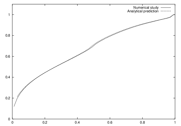
The function F⁡(R)F(R) is plotted in figure 1.

Remark 1.3.

If star graphs satisfied quantum ergodicity, then F⁡(R)F(R) would be the step-function

F⁡(R)={1,for R>1/α0,for R<1/αF(R)=\left\{\begin{array}[]{ll}1,&\mbox{for $R>1/\alpha$}\\ 0,&\mbox{for $R<1/\alpha$}\end{array}\right. (1.5)

for this observable.

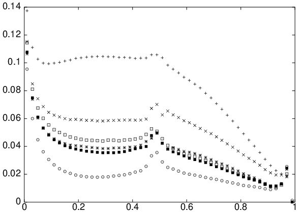
In figure 1 we compare the numerical data for the value distribution of ⟨𝝍(n)|𝐁|𝝍(n)⟩\langle{\boldsymbol{\psi}}^{(n)}|{\bf{B}}|{\boldsymbol{\psi}}^{(n)}\rangle for a star graph with 90 bonds with the v→∞v\to\infty analytical prediction F⁡(R)F(R). The difference between the actual distribution F⁡(R)F(R) and that which would be expected if the graph were quantum ergodic (remark 1.3) is clear. Figure 2 shows the difference between numerical data and F⁡(R)F(R) for increasing values of vv.

We we also show that for graphs with fixed number of bonds, there are subsequences of eigenfunctions that localise on two bonds.

Theorem 1.4.

Let the elements of 𝐋{\bf{L}} be linearly independent over ℚ{\mathbb{Q}}. Given any distinct two bonds, indexed by i1i_{1} and i2i_{2}, of a vv-bond star graph, there exists a subsequence (knr)⊆(kn)(k_{n_{r}})\subseteq(k_{n}) such that for any 𝐟=(fi)i=1v{\bf{f}}=(f_{i})_{i=1}^{v} smooth in each component,

limr→∞⟨𝝍(nr)|𝐟|𝝍(nr)⟩=1Li1+Li2​(∫0Li1fi1​(x)​𝑑x+∫0Li2fi2​(x)​𝑑x).\lim_{r\to\infty}\langle{\boldsymbol{\psi}}^{(n_{r})}|{\bf{f}}|{\boldsymbol{\psi}}^{(n_{r})}\rangle=\frac{1}{L_{i_{1}}+L_{i_{2}}}\left(\int_{0}^{L_{i_{1}}}f_{i_{1}}(x){\mathrm{d}}x+\int_{0}^{L_{i_{2}}}f_{i_{2}}(x){\mathrm{d}}x\right). (1.6)
Refer to caption
Figure 1: Comparing numerical data with the analytical prediction, F⁡(R)F(R). For this plot α=3\alpha=3 and in the numerical study, v=30v=30.
Refer to caption
Figure 2: Convergence to F⁡(R)F(R) for v=5(+),10(×),15(+×),20(⊡),25(■),30(⊙)v=5(+),10(\times),15(+\mspace{-14mu}\times),20(\boxdot),25(\blacksquare),30(\odot).

2 Quantum Star Graphs

A star graph11 1 sometimes referred to as a Hydra graph is a metric graph with bb vertices all connected only to one central vertex. Thus there are b+1b+1 vertices and bb bonds (figure 3). We shall denote by 𝐋∈ℝb{\bf{L}}\in{\mathbb{R}}^{b} the vector of bond lengths.

Refer to caption
Figure 3: A star graph with 5 bonds

We define the quantum star graph in the following way. Let ℋ\mathcal{H} denote the real Hilbert space

ℋ:=L2([0,L1])×⋯×L2([0,Lb])\mathcal{H}:=L^{2}([0,L_{1}])\times\cdots\times L^{2}([0,L_{b}]) (2.7)

with inner product

⟨𝐟|𝐠⟩:=∑j=1b∫0Ljfj​(x)​gj​(x)​𝑑x.\langle{\bf{f}}|{\bf{g}}\rangle:=\sum_{j=1}^{b}\int_{0}^{L_{j}}f_{j}(x)g_{j}(x){\mathrm{d}}{x}. (2.8)

Elements of ℋ\mathcal{H} are denoted 𝐟=(f1,…,fb){\bf{f}}=(f_{1},\ldots,f_{b}). Let ℱ⊆ℋ\mathcal{F}\subseteq\mathcal{H} be the subset of functions 𝐟{\bf{f}} which are twice-differentiable in each component and satisfy the conditions

fj​(0)=fi​(0)\displaystyle f_{j}(0)=f_{i}(0) =:\displaystyle=: f0,j,i=1,…,b\displaystyle f_{0},\qquad j,i=1,\ldots,b (2.9)
∑j=1bfj′​(0)\displaystyle\sum_{j=1}^{b}f_{j}^{\prime}(0) =\displaystyle= 1λ​f0\displaystyle\frac{1}{\lambda}f_{0} (2.10)
fj′​(Lj)\displaystyle f_{j}^{\prime}(L_{j}) =\displaystyle= 0,j=1,…,b.\displaystyle 0,\qquad j=1,\ldots,b. (2.11)

The parameter λ\lambda may be varied to give different boundary conditions at the central vertex of the graph. Henceforth we shall concentrate on the case 1/λ=01/\lambda=0, the so-called Neumann condition. The Laplace operator △\triangle on ℱ\mathcal{F} is defined by

△​𝐟:=(d2​f1d​x2,…,d2​fbd​x2).\triangle{\bf{f}}:=\left(\frac{{\mathrm{d}}^{2}f_{1}}{{\mathrm{d}}x^{2}},\ldots,\frac{{\mathrm{d}}^{2}{f_{b}}}{{\mathrm{d}}x^{2}}\right). (2.12)

△\triangle defined on ℱ\mathcal{F} is self-adjoint. Since the space on which the functions in ℱ\mathcal{F} are defined is compact, the operator △\triangle has a discrete spectrum of eigenvalues ([DS], Section XIII.4). i.e. the equation

−△​𝝍=k2​𝝍-\triangle{\boldsymbol{\psi}}=k^{2}{\boldsymbol{\psi}} (2.13)

has non-trivial solutions for k=k1,k2,…k=k_{1},k_{2},\ldots Such 𝝍{\boldsymbol{\psi}} are the wave-functions [KS1, KS2]. We shall use the notation that 𝝍(n):=(ψi(n)​(x))i=1b{\boldsymbol{\psi}}^{(n)}:=(\psi_{i}^{(n)}(x))_{i=1}^{b} is the wave-function corresponding to k=knk=k_{n}.

Solving (2.13) with boundary conditions (2.9)–(2.11), we find that the component of the nthn^{\rm th} normalised eigenfunction of the Laplace operator on the ithi^{\rm th} bond of a star graph is

ψi(n)(x)=Ai(n)coskn(x−Li)\psi_{i}^{(n)}(x)=A_{i}^{(n)}\cos k_{n}(x-L_{i}) (2.14)

where the amplitude is given by

Ai(n)=(2​sec2⁡kn​Li∑j=1bLj​sec2⁡kn​Lj)1/2A_{i}^{(n)}=\left(\frac{2\sec^{2}k_{n}L_{i}}{\sum_{j=1}^{b}L_{j}\sec^{2}{k_{n}L_{j}}}\right)^{1/2} (2.15)

and knk_{n} is the nthn^{\rm th} positive solution to

Z⁡(k,𝐋):=∑j=1btan⁡k​Lj=0.Z(k,{\bf{L}}):=\sum_{j=1}^{b}\tan kL_{j}=0. (2.16)

In sections 3–5 it will be convenient to take b=α​vb=\alpha v, where α∈ℕ\alpha\in{\mathbb{N}} is fixed. This is so that we can easily describe a fraction of the total number of bonds as the number of bonds becomes large (v→∞v\to\infty). In section 6 we shall take α=1\alpha=1 for notational convenience, since there we will only be concerned with fixed graphs.

3 Distribution of the observable 𝐁{\bf{B}}

In this section we prove the existence of a limit distribution for the diagonal matrix elements of 𝐁{\bf{B}} on star graphs with a fixed number, α​v\alpha v of bonds.

Lemma 3.1.

Consider a star graph with α​v\alpha v bonds with fixed lengths given by the vector 𝐋{\bf{L}}. Then for 𝐁{\bf{B}} defined by (1.1),

⟨𝝍(n)|𝐁|𝝍(n)⟩=∑i=1vLi​sec2⁡kn​Li∑j=1α​vLj​sec2⁡kn​Lj+O⁡(1kn)\langle{\boldsymbol{\psi}}^{(n)}|{\bf{B}}|{\boldsymbol{\psi}}^{(n)}\rangle=\frac{\sum_{i=1}^{v}L_{i}\sec^{2}{k_{n}L_{i}}}{\sum_{j=1}^{\alpha v}L_{j}\sec^{2}k_{n}L_{j}}+{\mathrm{O}}\left(\frac{1}{k_{n}}\right) (3.17)

where the error estimate is uniform in vv and Li⩾Lmin>0L_{i}\geqslant L_{\rm min}>0 for each ii.

Proof.XWe recall that

⟨𝝍(n)|𝐁|𝝍(n)⟩=∑j=1α​v∫0Lj|ψj(n)​(x)|2​Bj​(x)​𝑑x.\langle{\boldsymbol{\psi}}^{(n)}|{\bf{B}}|{\boldsymbol{\psi}}^{(n)}\rangle=\sum_{j=1}^{\alpha v}\int_{0}^{L_{j}}|\psi_{j}^{(n)}(x)|^{2}B_{j}(x){\mathrm{d}}x. (3.18)

Integrating (2.14) gives, for i=1,…,vi=1,\ldots,v,

∫0Li|ψi(n)(x)|2Bi(x)dx=1∑j=1α​vLj​sec2⁡kn​Lj(Lisec2knLi+1kntanknLi),\int_{0}^{L_{i}}|\psi_{i}^{(n)}(x)|^{2}B_{i}(x){\mathrm{d}}x=\frac{1}{\sum_{j=1}^{\alpha v}L_{j}\sec^{2}{k_{n}L_{j}}}\left(L_{i}\sec^{2}k_{n}L_{i}+\frac{1}{k_{n}}\tan k_{n}L_{i}\right), (3.19)

and for i⩾v+1i\geqslant v+1,

∫0Li|ψi(n)​(x)|2​Bi​(x)​𝑑x=0.\int_{0}^{L_{i}}|\psi_{i}^{(n)}(x)|^{2}B_{i}(x){\mathrm{d}}x=0. (3.20)

Thus

⟨𝝍(n)|𝐁|𝝍(n)⟩=∑i=1vLi​sec2⁡kn​Li∑j=1α​vLj​sec2⁡kn​Lj+Ekn\langle{\boldsymbol{\psi}}^{(n)}|{\bf{B}}|{\boldsymbol{\psi}}^{(n)}\rangle=\frac{\sum_{i=1}^{v}L_{i}\sec^{2}{k_{n}L_{i}}}{\sum_{j=1}^{\alpha v}L_{j}\sec^{2}k_{n}L_{j}}+\frac{E}{k_{n}} (3.21)

where

E=∑i=1vtan⁡kn​Li∑j=1α​vLj​sec2⁡kn​Lj.E=\frac{\sum_{i=1}^{v}\tan{k_{n}L_{i}}}{\sum_{j=1}^{\alpha v}L_{j}\sec^{2}k_{n}L_{j}}. (3.22)

Let Lmin:=minj⁡{Lj}L_{\rm min}:=\min_{j}\{L_{j}\}. Then

|E|\displaystyle|E| ⩽\displaystyle\leqslant ∑i=1v|tan⁡kn​Li|(α−1)​Lmin​v+Lmin​∑j=1vsec2⁡kn​Lj\displaystyle\frac{\sum_{i=1}^{v}|\tan{k_{n}L_{i}}|}{(\alpha-1)L_{\rm min}v+L_{\rm min}\sum_{j=1}^{v}\sec^{2}k_{n}L_{j}} (3.23)
⩽\displaystyle\leqslant (Lmin+(α−1)​v​Lmin∑i=1vsec2⁡kn​Lj)−1\displaystyle\left(L_{\rm min}+\frac{(\alpha-1)vL_{\rm min}}{\sum_{i=1}^{v}\sec^{2}{k_{n}L_{j}}}\right)^{-1} (3.24)

using the fact that |tan⁡θ|⩽sec2⁡θ|\tan\theta|\leqslant\sec^{2}\theta for any θ∈ℝ\theta\in{\mathbb{R}}. Hence E=O⁡(1)E={\mathrm{O}}(1) as n→∞n\to\infty uniformly in vv, Lmin>0L_{\rm min}>0. □\Box

Proof of theorem 1.1.X By lemma 3.1,

h⁡(⟨𝝍(n)|𝐁|𝝍(n)⟩)=h⁡(∑i=1vLi​sec2⁡xi∑j=1α​vLj​sec2⁡xj)+Enh(\langle{\boldsymbol{\psi}}^{(n)}|{\bf{B}}|{\boldsymbol{\psi}}^{(n)}\rangle)=h\left(\frac{\sum_{i=1}^{v}L_{i}\sec^{2}{x_{i}}}{\sum_{j=1}^{\alpha v}L_{j}\sec^{2}x_{j}}\right)+E_{n} (3.25)

where En=o⁡(1)E_{n}={\mathrm{o}}(1) as n→∞n\to\infty since hh is uniformly continuous on [0,1][0,1]. Hence

1N​∑n=1NEn→0as N→∞.\frac{1}{N}\sum_{n=1}^{N}E_{n}\to 0\quad\mbox{as $N\to\infty$.} (3.26)

Therefore

limN→∞1N​∑n=1Nh⁡(⟨𝝍(n)|𝐁|𝝍(n)⟩)=limN→∞1N​∑n=1Nh⁡(∑i=1vLi​sec2⁡kn​Li∑j=1α​vLj​sec2⁡kn​Lj).\lim_{N\to\infty}\frac{1}{N}\sum_{n=1}^{N}h(\langle{\boldsymbol{\psi}}^{(n)}|{\bf{B}}|{\boldsymbol{\psi}}^{(n)}\rangle)=\lim_{N\to\infty}\frac{1}{N}\sum_{n=1}^{N}h\left(\frac{\sum_{i=1}^{v}L_{i}\sec^{2}{k_{n}L_{i}}}{\sum_{j=1}^{\alpha v}L_{j}\sec^{2}k_{n}L_{j}}\right). (3.27)

According to Barra and Gaspard, there is an absolutely continuous measure ν⁡(𝝃)\nu({\boldsymbol{\xi}}) such that for piecewise continuous functions, f:Σ→ℝf:\Sigma\to{\mathbb{R}},

limN→∞1N​∑n=1Nf⁡(kn​𝐋)=∫Σf⁡(𝝃)​𝑑ν​(𝝃)\lim_{N\to\infty}\frac{1}{N}\sum_{n=1}^{N}f(k_{n}{\bf{L}})=\int_{\Sigma}f({\boldsymbol{\xi}}){\mathrm{d}}\nu({\boldsymbol{\xi}})

where Σ\Sigma is the surface embedded in the α​v\alpha v dimensional torus with side π\pi, defined by

tan⁡x1+⋯+tan⁡xα​v=0.\tan x_{1}+\cdots+\tan x_{\alpha v}=0.

𝝃{\boldsymbol{\xi}} is a set of α​v−1\alpha v-1 coordinates which parameterise Σ\Sigma. To avoid repetition, we refer the reader to [BG], [KMW] for more detail about this result and its application to similar problems.

Let

f⁡(𝐱)=h⁡(∑i=1vLi​sec2⁡xi∑j=1α​vLj​sec2⁡xj)f({\bf{x}})=h\left(\frac{\sum_{i=1}^{v}L_{i}\sec^{2}{x_{i}}}{\sum_{j=1}^{\alpha v}L_{j}\sec^{2}x_{j}}\right) (3.28)

we can define pv​(η)p_{v}(\eta) by

∫Σf⁡(𝝃)​𝑑ν​(𝝃)=:∫−∞∞h⁡(η)​pv​(η)​𝑑η.\int_{\Sigma}f({\boldsymbol{\xi}}){\mathrm{d}}\nu({\boldsymbol{\xi}})=:\int_{-\infty}^{\infty}h(\eta)p_{v}(\eta){\mathrm{d}}\eta. (3.29)

Since 0⩽⟨𝝍(n)|𝐁|𝝍(n)⟩⩽10\leqslant\langle{\boldsymbol{\psi}}^{(n)}|{\bf{B}}|{\boldsymbol{\psi}}^{(n)}\rangle\leqslant 1, it follows that pv​(η)p_{v}(\eta) is supported on [0,1][0,1]. □\Box

4 The large graph limit

Let η∈ℝ\eta\in{\mathbb{R}} and define

Xη​(n):=1v2​∑j=v+1α​vLj​sec2⁡kn​Lj−ηv2​∑i=1vLi​sec2⁡kn​LiX_{\eta}(n):=\frac{1}{v^{2}}\sum_{j=v+1}^{\alpha v}L_{j}\sec^{2}k_{n}L_{j}-\frac{\eta}{v^{2}}\sum_{i=1}^{v}L_{i}\sec^{2}k_{n}L_{i} (4.30)

for n=1,2,…n=1,2,\ldots\; The key result of this section is the following.

Proposition 4.1.

For each vv, there exists a probability density function fXη,vf_{X_{\eta},v} such that

limN→∞1N​#​{n∈{1,…,N}:Xη​(n)<S}=∫−∞SfXη,v​(σ)​𝑑σ.\lim_{N\to\infty}\frac{1}{N}\#\left\{n\in\{1,\ldots,N\}:X_{\eta}(n)<S\right\}=\int_{-\infty}^{S}f_{X_{\eta},v}(\sigma){\mathrm{d}}\sigma. (4.31)

Furthermore, for each S∈ℝS\in{\mathbb{R}},

∫−∞SfXη,v​(σ)​𝑑σ→∫−∞SfXη​(σ)​𝑑σ\int_{-\infty}^{S}f_{X_{\eta},v}(\sigma){\mathrm{d}}\sigma\to\int_{-\infty}^{S}f_{X_{\eta}}(\sigma){\mathrm{d}}\sigma

as v→∞v\to\infty, provided that v​Δ​L→0v\Delta L\to 0 in this limit, where

fXη​(σ)=−14​α​π​ℜ​𝔢​∫−∞∞Pη​(ξ)​e3​i​π/4​τη​(ξ)(−σ)3/2​w​(e3​i​π/4​τη​(ξ)2​−σ)​𝑑ξ.f_{X_{\eta}}(\sigma)=\frac{-1}{4\alpha\sqrt{\pi}}{\mathfrak{Re}}\int_{-\infty}^{\infty}P_{\eta}(\xi)\frac{{\mathrm{e}}^{3{\mathrm{i}}\pi/4}\tau_{\eta}(\xi)}{(-\sigma)^{3/2}}w\left(\frac{{\mathrm{e}}^{3{\mathrm{i}}\pi/4}\tau_{\eta}(\xi)}{2\sqrt{-\sigma}}\right){\mathrm{d}}\xi.

The functions PηP_{\eta} and τη\tau_{\eta} are defined by (4.43) and (4.44) below, and w⁡(z):=e−z2​erfc(−i​z)w(z):={\mathrm{e}}^{-z^{2}}\mathop{\rm erfc}(-{\mathrm{i}}z).

Proof.XThe existence of the N→∞N\to\infty limiting density, fXη,vf_{X_{\eta},v} is a consequence of the result of Barra and Gaspard [BG]. The proof is entirely analogous to the proof of theorem 1.1.

We turn our attention to the v→∞v\to\infty limit of this density. With nn a random variable uniformly distributed on the set {1,…,N}\{1,\ldots,N\} for some N∈ℕN\in{\mathbb{N}}, the characteristic function for this random variable Xη​(n)X_{\eta}(n) is

ev,N​(β):=𝔼⁡(ei​β​Xη)=1N​∑n=1Nf⁡(kn​𝐋)+O⁡(v​Δ​L)e_{v,N}(\beta):={\mathbb{E}}({\mathrm{e}}^{{\mathrm{i}}\beta X_{\eta}})=\frac{1}{N}\sum_{n=1}^{N}f(k_{n}{\bf{L}})+{\mathrm{O}}(v\Delta L)

where f:[0,π]v→ℂf:[0,\pi]^{v}\to{\mathbb{C}} is defined to be

f⁡(𝐱):=exp⁡(i​βv2​(∑j=v+1α​vsec2⁡xj−η​∑i=1vsec2⁡xi)).f({\bf{x}}):=\exp\left(\frac{{\mathrm{i}}\beta}{v^{2}}\left(\sum_{j=v+1}^{\alpha v}\sec^{2}x_{j}-\eta\sum_{i=1}^{v}\sec^{2}x_{i}\right)\right).

Following the argument of [KMW] we can write

limN→∞\displaystyle\lim_{N\to\infty} 1N​∑n=1Nf⁡(kn​𝐋)\displaystyle\frac{1}{N}\sum_{n=1}^{N}f(k_{n}{\bf{L}})
=12​α​v21πα​v∫−∞∞∫0π⋯∫0π(∑j=1α​vsec2xj)f(𝐱)exp(i​ζv∑j=1α​vtanxj)dα​v𝐱dζ.\displaystyle=\frac{1}{2\alpha v^{2}}\frac{1}{\pi^{\alpha v}}\int_{-\infty}^{\infty}\int_{0}^{\pi}\!\cdots\!\int_{0}^{\pi}\left(\sum_{j=1}^{\alpha v}\sec^{2}x_{j}\right)f({\bf{x}})\exp\left(\frac{{\mathrm{i}}\zeta}{v}\sum_{j=1}^{\alpha v}\tan x_{j}\right){\mathrm{d}}^{\alpha v}{\bf{x}}{\mathrm{d}}\zeta.

Denoting this limit for each fixed v,βv,\beta by ev​(β)e_{v}(\beta), we can write

ev​(β)=12​α​v​∫−∞∞I1​I2v−1​I3α​v−v+(α−1)​I4​I2v​I3α​v−v−1​𝑑ζe_{v}(\beta)=\frac{1}{2\alpha v}\int_{-\infty}^{\infty}I_{1}I_{2}^{v-1}I_{3}^{\alpha v-v}+(\alpha-1)I_{4}I_{2}^{v}I_{3}^{\alpha v-v-1}{\mathrm{d}}\zeta (4.32)

where the integrals I1,…,I4I_{1},\ldots,I_{4} are:-

I1\displaystyle I_{1} :⁣=\displaystyle:= 1π​∫0πsec2⁡x​exp⁡(i​ζv​tan⁡x−i​β​ηv2​sec2⁡x)​𝑑x,\displaystyle\frac{1}{\pi}\int_{0}^{\pi}\sec^{2}x\exp\left(\frac{{\mathrm{i}}\zeta}{v}\tan x-\frac{{\mathrm{i}}\beta\eta}{v^{2}}\sec^{2}x\right){\mathrm{d}}x, (4.33)
I2\displaystyle I_{2} :⁣=\displaystyle:= 1π​∫0πexp⁡(i​ζv​tan⁡x−i​β​ηv2​sec2⁡x)​𝑑x,\displaystyle\frac{1}{\pi}\int_{0}^{\pi}\exp\left(\frac{{\mathrm{i}}\zeta}{v}\tan x-\frac{{\mathrm{i}}\beta\eta}{v^{2}}\sec^{2}x\right){\mathrm{d}}x, (4.34)
I3\displaystyle I_{3} :⁣=\displaystyle:= 1π​∫0πexp⁡(i​ζv​tan⁡x+i​βv2​sec2⁡x)​𝑑x,\displaystyle\frac{1}{\pi}\int_{0}^{\pi}\exp\left(\frac{{\mathrm{i}}\zeta}{v}\tan x+\frac{{\mathrm{i}}\beta}{v^{2}}\sec^{2}x\right){\mathrm{d}}x, (4.35)
I4\displaystyle I_{4} :⁣=\displaystyle:= 1π​∫0πsec2⁡x​exp⁡(i​ζv​tan⁡x+i​βv2​sec2⁡x)​𝑑x.\displaystyle\frac{1}{\pi}\int_{0}^{\pi}\sec^{2}x\exp\left(\frac{{\mathrm{i}}\zeta}{v}\tan x+\frac{{\mathrm{i}}\beta}{v^{2}}\sec^{2}x\right){\mathrm{d}}x. (4.36)

An integral similar to (4.32) was tackled in [KMW]. We quote here the relevant results, mutatis mutandis. Asymptotic analysis of the integrals in (4.33–4.36) gives

I1=vπ​β​η​exp⁡(−i​π4+i​ζ24​β​η)+O⁡(1)as v→∞I_{1}=\frac{v}{\sqrt{\pi\beta\eta}}\exp\left(-\frac{{\mathrm{i}}\pi}{4}+\frac{{\mathrm{i}}\zeta^{2}}{4\beta\eta}\right)+{\mathrm{O}}(1)\quad\mbox{as $v\to\infty$} (4.37)

and

I4=vπ​β​exp⁡(i​π4−i​ζ24​β)+O⁡(1)as v→∞.I_{4}=\frac{v}{\sqrt{\pi\beta}}\exp\left(\frac{{\mathrm{i}}\pi}{4}-\frac{{\mathrm{i}}\zeta^{2}}{4\beta}\right)+{\mathrm{O}}(1)\quad\mbox{as $v\to\infty$}. (4.38)

For I2I_{2} and I3I_{3} we consider separately the cases −v<ζ<v-\sqrt{v}<\zeta<\sqrt{v} and |ζ|>v|\zeta|>\sqrt{v}. For −v<ζ<v-\sqrt{v}<\zeta<\sqrt{v},

I2v=exp⁡(−2π​β​η​exp⁡(i​π4+i​ζ24​β​η)−ζ​erf(e−iπ/4ζ2​β​η))​(1+O⁡(1+ζ2v))I_{2}^{v}=\exp\left(-\frac{2}{\sqrt{\pi}}\sqrt{\beta\eta}\exp\left(\frac{{\mathrm{i}}\pi}{4}+\frac{{\mathrm{i}}\zeta^{2}}{4\beta\eta}\right)-\zeta\mathop{\rm erf}\left(\frac{{\mathrm{e}}^{-{\mathrm{i}}\pi/4}\zeta}{2\sqrt{\beta\eta}}\right)\right)\left(1+{\mathrm{O}}\left(\frac{1+\zeta^{2}}{v}\right)\right) (4.39)

and

I3(α−1)​v=exp(−2​(α−1)πβexp(−i​π4−i​ζ24​β)−ζ(α−1)erf\displaystyle I_{3}^{(\alpha-1)v}=\exp\left(-\frac{2(\alpha-1)}{\sqrt{\pi}}\sqrt{\beta}\exp\left(-\frac{{\mathrm{i}}\pi}{4}-\frac{{\mathrm{i}}\zeta^{2}}{4\beta}\right)-\zeta(\alpha-1)\right.\mathop{\rm erf} OPEN(ei​π/4​ζ2​β))\displaystyle\left.\left(\frac{{\mathrm{e}}^{{\mathrm{i}}\pi/4}\zeta}{2\sqrt{\beta}}\right)\right) (4.40)
×(1+O⁡(1+ζ2v)),\displaystyle\times\left(1+{\mathrm{O}}\left(\frac{1+\zeta^{2}}{v}\right)\right),

both error estimates are as v→∞v\to\infty. For |ζ|>v|\zeta|>\sqrt{v},

|I2|⩽β​ηv​π​(β​ηv2+ζ2β​η)−1+O⁡(ζ−3)|I_{2}|\leqslant\frac{\sqrt{\beta\eta}}{v\pi}\left(\frac{\beta\eta}{v^{2}}+\frac{\zeta^{2}}{\beta\eta}\right)^{-1}+{\mathrm{O}}(\zeta^{-3}) (4.41)

as ζ→∞\zeta\to\infty, and

|I3|⩽βv​π​(βv2+ζ2β)−1+O⁡(ζ−3).|I_{3}|\leqslant\frac{\sqrt{\beta}}{v\pi}\left(\frac{\beta}{v^{2}}+\frac{\zeta^{2}}{\beta}\right)^{-1}+{\mathrm{O}}(\zeta^{-3}). (4.42)

Using these estimates, we can find an expression for the limit of ev​(β)e_{v}(\beta) as v→∞v\to\infty,

e⁡(β):=limv→∞ev​(β)\displaystyle e(\beta):=\lim_{v\to\infty}e_{v}(\beta) =12​α​∫−∞∞1β​Pη​(ζβ)​exp⁡(−β​τη​(ζβ))​𝑑ζ\displaystyle=\frac{1}{2\alpha}\int_{-\infty}^{\infty}\frac{1}{\sqrt{\beta}}P_{\eta}\left(\frac{\zeta}{\sqrt{\beta}}\right)\exp\left(-\sqrt{\beta}\tau_{\eta}\left(\frac{\zeta}{\sqrt{\beta}}\right)\right){\mathrm{d}}\zeta
=∫−∞∞Pη​(ξ)​exp⁡(−β​τη​(ξ))​𝑑ξ.\displaystyle=\int_{-\infty}^{\infty}P_{\eta}(\xi)\exp\left(-\sqrt{\beta}\tau_{\eta}(\xi)\right){\mathrm{d}}\xi.

For ease of notation, we have introduced

Pη​(ξ):=1π​η​exp⁡(−i​π4+i​ξ24​η)+(α−1)π​exp⁡(i​π4−i​ξ24)P_{\eta}(\xi):=\frac{1}{\sqrt{\pi\eta}}\exp\left(\frac{-{\mathrm{i}}\pi}{4}+\frac{{\mathrm{i}}\xi^{2}}{4\eta}\right)+\frac{(\alpha-1)}{\sqrt{\pi}}\exp\left(\frac{{\mathrm{i}}\pi}{4}-\frac{{\mathrm{i}}\xi^{2}}{4}\right) (4.43)

and

τη​(ξ):=\displaystyle\tau_{\eta}(\xi):= 2π​η​exp⁡(i​π4+i​ξ24​η)+ξ​erf(e−iπ/4ξ2​η)\displaystyle\frac{2}{\sqrt{\pi}}\sqrt{\eta}\exp\left(\frac{{\mathrm{i}}\pi}{4}+\frac{{\mathrm{i}}\xi^{2}}{4\eta}\right)+\xi\mathop{\rm erf}\left(\frac{{\mathrm{e}}^{-{\mathrm{i}}\pi/4}\xi}{2\sqrt{\eta}}\right)
+2​(α−1)π​exp⁡(−i​π4−i​ξ24)+ξ⁡(α−1)​erf(ei​π/4​ξ2).\displaystyle+\frac{2(\alpha-1)}{\sqrt{\pi}}\exp\left(-\frac{{\mathrm{i}}\pi}{4}-\frac{{\mathrm{i}}\xi^{2}}{4}\right)+\xi(\alpha-1)\mathop{\rm erf}\left(\frac{{\mathrm{e}}^{{\mathrm{i}}\pi/4}\xi}{2}\right). (4.44)

In the above, wherever β\sqrt{\beta} occurs for β<0\beta<0, this should be understood to mean ±i​−β\pm{\mathrm{i}}\sqrt{-\beta} where the sign is taken in such a way that

e⁡(−β)=e⁡(β)¯,e(-\beta)=\overline{e(\beta)},

the usual condition for the characteristic function of a probability density. This can always be done. We also note that e⁡(0)=1e(0)=1 which is consistent with e⁡(β)e(\beta) being the characteristic function of a probability distribution. e⁡(β)e(\beta) is continuous at β=0\beta=0 since the defining integral is uniformly convergent in β\beta (see lemma A.3 below). Thus the limiting density, fXηf_{X_{\eta}} exists and is given by

fXη​(σ)=12​π​∫−∞∞12​α​∫−∞∞Pη​(ξ)​exp⁡(−β​τη​(ξ)−i​σ​β)​𝑑ξ​𝑑β,f_{X_{\eta}}(\sigma)=\frac{1}{2\pi}\int_{-\infty}^{\infty}\frac{1}{2\alpha}\int_{-\infty}^{\infty}P_{\eta}(\xi)\exp(-\sqrt{\beta}\tau_{\eta}(\xi)-{\mathrm{i}}\sigma\beta){\mathrm{d}}\xi{\mathrm{d}}\beta, (4.45)

where we have made the substitution ξ=ζ/β\xi=\zeta/\sqrt{\beta}. We here switch the order of integration. This is a non-trivial operation since both integrals are improper. However in this case we can rigorously justify the manoeuvre. Justification is provided in appendix A, proposition A.8.

fXη​(σ)\displaystyle f_{X_{\eta}}(\sigma) =\displaystyle= 12​π​α​ℜ​𝔢​∫−∞∞Pη​(ξ)​∫0∞exp⁡(−β​τη​(ξ)−i​σ​β)​𝑑β​𝑑ξ\displaystyle\frac{1}{2\pi\alpha}{\mathfrak{Re}}\int_{-\infty}^{\infty}P_{\eta}(\xi)\int_{0}^{\infty}\exp(-\sqrt{\beta}\tau_{\eta}(\xi)-{\mathrm{i}}\sigma\beta){\mathrm{d}}\beta\;{\mathrm{d}}\xi (4.46)
=\displaystyle= 12​π​α​ℜ​𝔢​∫−∞∞Pη​(ξ)​(1i​σ−π2​e3​i​π/4​τη​(ξ)(−σ)3/2​w​(e3​i​π/4​τη​(ξ)2​−σ))​𝑑ξ.\displaystyle\frac{1}{2\pi\alpha}{\mathfrak{Re}}\int_{-\infty}^{\infty}P_{\eta}(\xi)\left(\frac{1}{{\mathrm{i}}\sigma}-\frac{\sqrt{\pi}}{2}\frac{{\mathrm{e}}^{3{\mathrm{i}}\pi/4}\tau_{\eta}(\xi)}{(-\sigma)^{3/2}}w\left(\frac{{\mathrm{e}}^{3{\mathrm{i}}\pi/4}\tau_{\eta}(\xi)}{2\sqrt{-\sigma}}\right)\right){\mathrm{d}}\xi.

To evaluate the final integration we have used the following result (a variant of formula 3.462.5 in [GR]),

∫0∞exp⁡(−a​x−b​x)​𝑑x=1a−π2​ba3/2​w​(i​b2​a1/2).\int_{0}^{\infty}\exp(-ax-b\sqrt{x}){\mathrm{d}}x=\frac{1}{a}-\frac{\sqrt{\pi}}{2}\frac{b}{a^{3/2}}w\left(\frac{{\mathrm{i}}b}{2a^{1/2}}\right). (4.47)

To conclude we observe that since

∫−∞∞Pη​(ξ)​𝑑ξ=2​α∈ℝ\int_{-\infty}^{\infty}P_{\eta}(\xi){\mathrm{d}}\xi=2\alpha\in{\mathbb{R}}

the first term in (4.46) vanishes as it has zero real part. □\Box

Some properties of w⁡(z)w(z) are discussed in [AS] chapter 7. We shall use the following

Lemma 4.2.

The function w⁡(z)w(z) has the asymptotic expansion

w⁡(z)∼iπ​∑m=0∞(2​m)!4m​m!​z2​m+1w(z)\sim\frac{{\mathrm{i}}}{\sqrt{\pi}}\sum_{m=0}^{\infty}\frac{(2m)!}{4^{m}m!z^{2m+1}} (4.48)

as z→∞z\to\infty, valid for −π4<arg⁡z<5​π4\displaystyle\frac{-\pi}{4}<\arg z<\frac{5\pi}{4}.

Proof.XThis follows from the asymptotic expansion of erfc\mathop{\rm erfc},

π​z​ez2​erfc(z)∼∑m=0∞(2​m)!(4​z2)m​m!,\sqrt{\pi}z{\mathrm{e}}^{z^{2}}\mathop{\rm erfc}(z)\sim\sum_{m=0}^{\infty}\frac{(2m)!}{(4z^{2})^{m}m!},

as z→∞z\to\infty, |arg⁡z|<3​π/4|\arg z|<3\pi/4, taken from [AS] (formula 7.1.23; see also [BlHa] exercise 3.11). The series for ww comes from making the substitution z↦−i​zz\mapsto-{\mathrm{i}}z. □\Box

Since erfc\mathop{\rm erfc} and ww are analytic functions, they are bounded in the domain of validity of their asymptotic expansions quoted in lemma 4.2.

Proposition 4.3.

Let z∈ℂz\in{\mathbb{C}} and −π/4<argz<5π/4-\pi/4<\arg z<5\pi/4. Then

∫0Rz​w​(z​p)​𝑑p=π2−arg⁡(z)π+iπ​log⁡|z|+i​CR+O⁡(1|z|2​R2)\int_{0}^{R}zw(zp){\mathrm{d}}p=\frac{\sqrt{\pi}}{2}-\frac{\arg(z)}{\sqrt{\pi}}+\frac{{\mathrm{i}}}{\sqrt{\pi}}\log|z|+{{\mathrm{i}}}C_{R}+{\mathrm{O}}\left(\frac{1}{|z|^{2}R^{2}}\right) (4.49)

where CR∈ℝC_{R}\in{\mathbb{R}} is independent of zz, but may depend on RR.

Proof.XWrite z=|z|​ei​φz=|z|{\mathrm{e}}^{{\mathrm{i}}\varphi} where φ=arg⁡z\varphi=\arg z. Then

∫0Rz​w​(z​p)​𝑑p=∫0|z|​Rei​φ​w​(ei​φ​p)​𝑑p\int_{0}^{R}zw(zp){\mathrm{d}}p=\int_{0}^{|z|R}{\mathrm{e}}^{{\mathrm{i}}\varphi}w({\mathrm{e}}^{{\mathrm{i}}\varphi}p){\mathrm{d}}p (4.50)

via p↦p/|z|p\mapsto p/|z|. Using Cauchy’s theorem,

∫0|z|​Rei​φ​w​(ei​φ​p)​𝑑p=∫γ1w⁡(t)​𝑑t=∫γ2w⁡(t)​𝑑t+∫γRw⁡(t)​𝑑t.\int_{0}^{|z|R}{\mathrm{e}}^{{\mathrm{i}}\varphi}w({\mathrm{e}}^{{\mathrm{i}}\varphi}p){\mathrm{d}}p=\int_{\gamma_{1}}w(t){\mathrm{d}}t=\int_{\gamma_{2}}w(t){\mathrm{d}}t+\int_{\gamma_{R}}w(t){\mathrm{d}}t. (4.51)

The contours γ1,γ2\gamma_{1},\gamma_{2} and γR\gamma_{R} in the complex tt-plane are illustrated in figure 4.

Figure 4: The contours γ1\gamma_{1}, γ2\gamma_{2} and γR\gamma_{R}.

On γ2\gamma_{2},

∫γ2w⁡(t)​𝑑t=\displaystyle\int_{\gamma_{2}}w(t){\mathrm{d}}t= ∫0|z|​Rw⁡(x)​𝑑x\displaystyle\int_{0}^{|z|R}w(x){\mathrm{d}}x
=\displaystyle= ∫01w⁡(x)​𝑑x+∫1|z|​R(w⁡(x)−iπ​x)​𝑑x+∫1|z|​Riπ​x​𝑑x\displaystyle\int_{0}^{1}w(x){\mathrm{d}}x+\int_{1}^{|z|R}\left(w(x)-\frac{{\mathrm{i}}}{\sqrt{\pi}x}\right){\mathrm{d}}x+\int_{1}^{|z|R}\frac{{\mathrm{i}}}{\sqrt{\pi}x}{\mathrm{d}}x
=\displaystyle= ∫01w⁡(x)​𝑑x+∫1∞(w⁡(x)−iπ​x)​𝑑x\displaystyle\int_{0}^{1}w(x){\mathrm{d}}x+\int_{1}^{\infty}\left(w(x)-\frac{{\mathrm{i}}}{\sqrt{\pi}x}\right){\mathrm{d}}x
−∫|z|​R∞(w(x)−iπ​x)dx+∫1|z|​Riπ​xdx\displaystyle-\int_{|z|R}^{\infty}\left(w(x)-\frac{{\mathrm{i}}}{\sqrt{\pi}x}\right){\mathrm{d}}x+\int_{1}^{|z|R}\frac{{\mathrm{i}}}{\sqrt{\pi}x}{\mathrm{d}}x
=\displaystyle= ∫0∞e−x2​𝑑x+i×const−∫|z|​R∞(w⁡(x)−iπ​x)​𝑑x+∫1|z|​Riπ​x​𝑑x,\displaystyle\int_{0}^{\infty}{\mathrm{e}}^{-x^{2}}{\mathrm{d}}x+{\mathrm{i}}\times\mbox{const}-\int_{|z|R}^{\infty}\left(w(x)-\frac{{\mathrm{i}}}{\sqrt{\pi}x}\right){\mathrm{d}}x+\int_{1}^{|z|R}\frac{{\mathrm{i}}}{\sqrt{\pi}x}{\mathrm{d}}x,

using w⁡(z)=e−x2​(1+i​erfiz)w(z)={\mathrm{e}}^{-x^{2}}(1+{\mathrm{i}}\mathop{\rm erf{}i}z) to separate the real and imaginary contributions. The imaginary part goes into the constant CRC_{R}, the value of which is not important since we shall always be considering only the real part of resulting expressions. By the use of lemma 4.2,

∫γ2w⁡(t)​𝑑t=π2+i×const+iπ​(log⁡R+log⁡|z|)+O⁡(1|z|2​R2)\int_{\gamma_{2}}w(t){\mathrm{d}}t=\frac{\sqrt{\pi}}{2}+{\mathrm{i}}\times\mbox{const}+\frac{{\mathrm{i}}}{\sqrt{\pi}}(\log R+\log|z|)+{\mathrm{O}}\left(\frac{1}{|z|^{2}R^{2}}\right) (4.52)

as R→∞R\to\infty uniformly for |z|⩾c|z|\geqslant c for some cc.

On γR\gamma_{R},

∫γRf⁡(t)​𝑑t\displaystyle\int_{\gamma_{R}}f(t){\mathrm{d}}t =\displaystyle= ∫0φi​|z|​R​ei​θ​w​(|z|​R​ei​θ)​𝑑θ\displaystyle\int_{0}^{\varphi}{\mathrm{i}}|z|R{\mathrm{e}}^{{\mathrm{i}}\theta}w(|z|R{\mathrm{e}}^{{\mathrm{i}}\theta}){\mathrm{d}}\theta (4.53)
=\displaystyle= ∫0φi​|z|​R​ei​θ​(−1π​i|z|R​ei​θ+O⁡(1|z|3​R3))by lemma 4.2\displaystyle\int_{0}^{\varphi}{\mathrm{i}}|z|R{\mathrm{e}}^{{\mathrm{i}}\theta}\left(\frac{-1}{\sqrt{\pi}{\mathrm{i}}|z|R{\mathrm{e}}^{{\mathrm{i}}\theta}}+{\mathrm{O}}\left(\frac{1}{|z|^{3}R^{3}}\right)\right)\quad\mbox{by lemma \ref{lem:w}}
=\displaystyle= −φπ+O⁡(1|z|2​R2).\displaystyle\frac{-\varphi}{\sqrt{\pi}}+{\mathrm{O}}\left(\frac{1}{|z|^{2}R^{2}}\right).

Combining (4.52) and (4.53) gives (4.49). □\Box

The following lemma from probability theory will also be useful.

Lemma 4.4.

Let U,VU,V be random variables, then

ℙ⁡(UV<η)=∫−∞0fXη​(σ)​𝑑σ{\mathbb{P}}\left(\frac{U}{V}<\eta\right)=\int_{-\infty}^{0}f_{X_{\eta}}(\sigma){\mathrm{d}}\sigma

where fXηf_{X_{\eta}} is the probability density function of the random variable Xη:=U−η​VX_{\eta}:=U-\eta V.

Proof.XThis follows immediately from the fact that

ℙ⁡(UV<η)=ℙ⁡(U−η​V<0).{\mathbb{P}}\left(\frac{U}{V}<\eta\right)={\mathbb{P}}(U-\eta V<0).

□\Box

5 Proof of theorem 1.2

We first observe that

∑i=1vLi​sec2⁡kn​Li∑j=1α​vLj​sec2⁡kn​Lj=(1+∑j=v+1α​vLj​sec2⁡kn​Lj∑1=1vLi​sec2⁡kn​Li)−1,\frac{\sum_{i=1}^{v}L_{i}\sec^{2}{k_{n}L_{i}}}{\sum_{j=1}^{\alpha v}L_{j}\sec^{2}k_{n}L_{j}}=\left(1+\frac{\sum_{j=v+1}^{\alpha v}L_{j}\sec^{2}{k_{n}L_{j}}}{\sum_{1=1}^{v}L_{i}\sec^{2}k_{n}L_{i}}\right)^{-1}, (5.54)

so we can concentrate on finding the probability distribution, F~​(η)\tilde{F}(\eta), of

∑j=v+1α​vLj​sec2⁡kn​Lj∑1=1vLi​sec2⁡kn​Li\frac{\sum_{j=v+1}^{\alpha v}L_{j}\sec^{2}{k_{n}L_{j}}}{\sum_{1=1}^{v}L_{i}\sec^{2}k_{n}L_{i}}

as v→∞v\to\infty. This will be then related to the distribution in which we are interested by a simple transformation (see equation (5.57) below). In light of lemma 4.4, F~​(η)\tilde{F}(\eta) is given by

F~​(η)=∫−∞0fXη​(σ)​𝑑σ\tilde{F}(\eta)=\int_{-\infty}^{0}f_{X_{\eta}}(\sigma){\mathrm{d}}\sigma

with fXηf_{X_{\eta}} found in proposition 4.1. It is more instructive to take the range of integration from −R2-R^{2} to 00, with a view to taking the limit R→∞R\to\infty later,

∫−R20fXη​(σ)​𝑑σ=−1π​α​ℜ​𝔢​∫−∞∞∫−R20Pη​(ξ)​e3​π​i/4​τη​(ξ)4​(−σ)3/2​w​(e3​π​i/4​τη​(ξ)−σ)​𝑑σ​𝑑ξ.\int_{-R^{2}}^{0}f_{X_{\eta}}(\sigma){\mathrm{d}}\sigma=\frac{-1}{\sqrt{\pi}\alpha}{\mathfrak{Re}}\int_{-\infty}^{\infty}\int_{-R^{2}}^{0}P_{\eta}(\xi)\frac{{\mathrm{e}}^{3\pi{\mathrm{i}}/4}\tau_{\eta}(\xi)}{4(-\sigma)^{3/2}}w\left(\frac{{\mathrm{e}}^{3\pi{\mathrm{i}}/4}\tau_{\eta}(\xi)}{\sqrt{-\sigma}}\right){\mathrm{d}}\sigma{\mathrm{d}}\xi. (5.55)

The ξ\xi-integral is uniformly convergent by lemma B.1, so we have legitimately switched the order of integration. We can then write

∫−R20fXη​(σ)​𝑑σ=\displaystyle\int_{-R^{2}}^{0}f_{X_{\eta}}(\sigma){\mathrm{d}}\sigma= −1α​π​ℜ​𝔢​∫−∞∞∫−∞0Pη​(ξ)​e3​π​i/4​τη​(ξ)4​(−σ)3/2​w​(e3​π​i/4​τη​(ξ)−σ)​𝑑σ​𝑑ξ\displaystyle\frac{-1}{\alpha\sqrt{\pi}}{\mathfrak{Re}}\int_{-\infty}^{\infty}\int_{-\infty}^{0}P_{\eta}(\xi)\frac{{\mathrm{e}}^{3\pi{\mathrm{i}}/4}\tau_{\eta}(\xi)}{4(-\sigma)^{3/2}}w\left(\frac{{\mathrm{e}}^{3\pi{\mathrm{i}}/4}\tau_{\eta}(\xi)}{\sqrt{-\sigma}}\right){\mathrm{d}}\sigma{\mathrm{d}}\xi
−−1π​αℜ𝔢∫−∞∞∫−∞−R2Pη(ξ)e3​π​i/4​τη​(ξ)4​(−σ)3/2w(e3​π​i/4​τη​(ξ)−σ)dσdξ.\displaystyle-\frac{-1}{\sqrt{\pi}\alpha}{\mathfrak{Re}}\int_{-\infty}^{\infty}\int_{-\infty}^{-R^{2}}P_{\eta}(\xi)\frac{{\mathrm{e}}^{3\pi{\mathrm{i}}/4}\tau_{\eta}(\xi)}{4(-\sigma)^{3/2}}w\left(\frac{{\mathrm{e}}^{3\pi{\mathrm{i}}/4}\tau_{\eta}(\xi)}{\sqrt{-\sigma}}\right){\mathrm{d}}\sigma{\mathrm{d}}\xi.

The second term vanishes as R→∞R\to\infty, as shown in proposition B.2. Making the substitution (−σ)−1/2=2p(-\sigma)^{-1/2}=2p, leads to

F~​(η)=−1π​α​ℜ​𝔢​∫−∞∞∫0∞Pη​(ξ)​e3​π​i/4​τη​(ξ)​w​(e3​π​i/4​τη​(ξ)​p)​𝑑p​𝑑ξ.\tilde{F}(\eta)=\frac{-1}{\sqrt{\pi}{\alpha}}{\mathfrak{Re}}\int_{-\infty}^{\infty}\int_{0}^{\infty}P_{\eta}(\xi){\mathrm{e}}^{3\pi{\mathrm{i}}/4}\tau_{\eta}(\xi)w({\mathrm{e}}^{3\pi{\mathrm{i}}/4}\tau_{\eta}(\xi)p){\mathrm{d}}p{\mathrm{d}}\xi.

We can apply proposition 4.3 with z=e3​i​π/4​τη​(ξ)z={\mathrm{e}}^{3{\mathrm{i}}\pi/4}\tau_{\eta}(\xi). We can integrate ξ\xi out of the error term provided by this proposition since

∫−∞∞1τη​(ξ)2​𝑑ξ<∞.\int_{-\infty}^{\infty}\frac{1}{\tau_{\eta}(\xi)^{2}}{\mathrm{d}}\xi<\infty.

We get, finally,

F~​(η)\displaystyle\tilde{F}(\eta) =\displaystyle= −1α​π​ℜ​𝔢​∫−∞∞Pη​(ξ)​(π2−arg⁡(e3​i​π/4​τη​(ξ))π+i​log⁡|τη​(ξ)|π)​𝑑ξ\displaystyle\frac{-1}{\alpha\sqrt{\pi}}{\mathfrak{Re}}\int_{-\infty}^{\infty}P_{\eta}(\xi)\left(\frac{\sqrt{\pi}}{2}-\frac{\arg({\mathrm{e}}^{3{\mathrm{i}}\pi/4}\tau_{\eta}(\xi))}{\sqrt{\pi}}+{\mathrm{i}}\frac{\log|\tau_{\eta}(\xi)|}{\sqrt{\pi}}\right){\mathrm{d}}\xi (5.56)
=\displaystyle= 12+1π​α​ℜ​𝔢​∫−∞∞Pη​(ξ)​(arg⁡(τη​(ξ))−i​log⁡|τη​(ξ)|)​𝑑ξ.\displaystyle\frac{1}{2}+\frac{1}{\pi\alpha}{\mathfrak{Re}}\int_{-\infty}^{\infty}P_{\eta}(\xi)\left(\arg(\tau_{\eta}(\xi))-{\mathrm{i}}\log|\tau_{\eta}(\xi)|\right){\mathrm{d}}\xi.

This is related to F⁡(η)F(\eta) by

F​(η)=1−F~​(1η−1).F(\eta)=1-\tilde{F}\left(\frac{1}{\eta}-1\right). (5.57)

□\Box

6 Scarred states on finite star graphs

We recall that theorem 1.4 is concerned with the quantity ⟨𝝍(n)|𝐟|𝝍(n)⟩\langle{\boldsymbol{\psi}}^{(n)}|{\bf{f}}|{\boldsymbol{\psi}}^{(n)}\rangle which can be written as

⟨𝝍(n)|𝐟|𝝍(n)⟩=∑i=1v∫0Li|ψi(n)​(x)|2​fi​(x)​𝑑x.\langle{\boldsymbol{\psi}}^{(n)}|{\bf{f}}|{\boldsymbol{\psi}}^{(n)}\rangle=\sum_{i=1}^{v}\int_{0}^{L_{i}}|\psi_{i}^{(n)}(x)|^{2}f_{i}(x){\mathrm{d}}x.

Now using (2.14) and the identity cos2⁡θ=1/2+(1/2)​cos⁡2​θ\cos^{2}\theta=1/2+(1/2)\cos 2\theta yields

⟨𝝍(n)|𝐟|𝝍(n)⟩=∑i=1vAi(n)22​(∫0Lifi​(x)​𝑑x+∫0Licos⁡2​kn​(x−Li)​fi​(x)​𝑑x).\langle{\boldsymbol{\psi}}^{(n)}|{\bf{f}}|{\boldsymbol{\psi}}^{(n)}\rangle=\sum_{i=1}^{v}\frac{{A_{i}^{(n)}}^{2}}{2}\left(\int_{0}^{L_{i}}f_{i}(x){\mathrm{d}}x+\int_{0}^{L_{i}}\cos 2k_{n}(x-L_{i})f_{i}(x){\mathrm{d}}x\right). (6.58)

Since we are interested in a subsequence knr→∞k_{n_{r}}\to\infty, we may hope that the second integrals do not survive. Thus our prime concern are the prefactors

Ai(n)2=2​sec2⁡kn​Li∑j=1vLj​sec2⁡kn​Lj.{A_{i}^{(n)}}^{2}=\frac{2\sec^{2}{k_{n}L_{i}}}{\sum_{j=1}^{v}L_{j}\sec^{2}{k_{n}L_{j}}}.

and to prove the theorem we need to find knk_{n} such that the prefactors are small for all ii other than (without loss of generality) 11 and 22.

To do this we study the poles of the function Z⁡(k,𝐋)Z(k,{\bf{L}}). Let

pn,i:=πLi​(12+n).p_{n,i}:=\frac{\pi}{L_{i}}\left(\frac{1}{2}+n\right).

Then |tan⁡p​Li|→∞|\tan pL_{i}|\to\infty and sec⁡p​Li→∞\sec pL_{i}\to\infty as p→pn,ip\to p_{n,i}.

Since the function Z⁡(k,𝐋)Z(k,{\bf{L}}) is an increasing function of kk, between any two poles there is a zero. We will use this important feature to “trap” zeros knrk_{n_{r}} of Z⁡(k,𝐋)Z(k,{\bf{L}}) between pairs of nearby poles pn,1p_{n,1} and pm,2p_{m,2}, also requiring that all other poles are far away (see Fig. 5). The implications will be that as r→∞r\to\infty,

sec2⁡knr​Li≫sec2⁡knr​Lj with ​i=1,2​ and ​j>2,\sec^{2}{k_{n_{r}}L_{i}}\gg\sec^{2}{k_{n_{r}}L_{j}}\qquad\mbox{ with }i=1,2\mbox{ and }j>2,

and

sec2⁡knr​L1∼sec2⁡knr​L2,\sec^{2}k_{n_{r}}L_{1}\sim\sec^{2}k_{n_{r}}L_{2},

ensuring that (1.6) holds.

To make the above arguments rigorous we need the following propositions.

Proposition 6.1.

Let the elements of 𝐋{\bf{L}} be linearly independent over ℚ{\mathbb{Q}}. Let 1<v∗<v1<v^{\ast}<v for v⩾3v\geqslant 3. Given ε>0\varepsilon>0 there exist infinitely many n∈ℕn\in{\mathbb{N}} such that

  • •

    for each i=2,…,v∗i=2,\ldots,v^{\ast} there exists m∈ℕm\in{\mathbb{N}} satisfying

    |pm,i−pn,1|⩽ε/2|p_{m,i}-p_{n,1}|\leqslant\varepsilon/2 (6.59)
  • •

    for all i=v∗+1,…,vi=v^{\ast}+1,\ldots,v and for all m∈ℕm\in{\mathbb{N}}

    |pm,i−pn,1|⩾π2​Li−ε/2.|p_{m,i}-p_{n,1}|\geqslant\frac{\pi}{2L_{i}}-\varepsilon/2. (6.60)

Proof.XThe idea behind the proof is that for linearly independent elements of 𝐋{\bf{L}} the poles p⋅,ip_{\cdot,i} for different ii behave like independent random variables, therefore every permitted pole configuration happens infinitely often. To substantiate this claim we express the nearest-pole distances as the states of an ergodic dynamical system.

For n∈ℕn\in{\mathbb{N}} and i=2,…,v∗i=2,\ldots,v^{\ast}, let δn,i\delta_{n,i} denote the distance between pn,1p_{n,1} and the closest pole of tan⁡k​Li\tan kL_{i};

δn,i:=pn,1−pm,i,\delta_{n,i}:=p_{n,1}-p_{m,i},

where mm is such that

|pm,i−pn,1|=minm⁡{|pm,i−pn,1|}.|p_{m,i}-p_{n,1}|=\min_{m}\{|p_{m,i}-p_{n,1}|\}.

Since the poles of tan⁡k​Li\tan kL_{i} are π/Li\pi/L_{i}-periodic, we have

δn,i+π2​Li\displaystyle\delta_{n,i}+\frac{\pi}{2L_{i}} =\displaystyle= pn,1−p0,i+π2​Limod​πLi\displaystyle p_{n,1}-p_{0,i}+\frac{\pi}{2L_{i}}\quad{\rm mod}\;\frac{\pi}{L_{i}} (6.61)
=\displaystyle= π2​L1+πL1​nmod​πLi.\displaystyle\frac{\pi}{2L_{1}}+\frac{\pi}{L_{1}}n\quad{\rm mod}\;\frac{\pi}{L_{i}}. (6.62)

Let ℓm,i\ell_{m,i} denote the mthm^{\rm th} zero of tan⁡k​Li\tan kL_{i}. We note that (6.60) is implied by the condition that

|ℓm,i−pn,1|⩽ε/2|\ell_{m,i}-p_{n,1}|\leqslant\varepsilon/2

for some m∈ℕm\in{\mathbb{N}}. For i=v∗+1,…,vi=v^{\ast}+1,\ldots,v, define ηn,i\eta_{n,i} to be the distance between pn,1p_{n,1} and the closest zero of tan⁡k​Li\tan kL_{i}. Similarly to (6.62)

ηn,i+π2​Li=π2​(1L1+1Li)+πL1​nmod​πLi.\eta_{n,i}+\frac{\pi}{2L_{i}}=\frac{\pi}{2}\left(\frac{1}{L_{1}}+\frac{1}{L_{i}}\right)+\frac{\pi}{L_{1}}n\quad{\rm mod}\;\frac{\pi}{L_{i}}. (6.63)

From (6.62) and (6.63), δn,i\delta_{n,i} and ηn,i\eta_{n,i} satisfy the recurrence

{δn+1,i=δn,i+πL1mod​πLii=2,…,v∗ηn+1,i=ηn,i+πL1mod​πLii=v∗+1,…,v\left\{\begin{array}[]{rcll}\delta_{n+1,i}&=&\delta_{n,i}+\frac{\pi}{L_{1}}\quad{\rm mod}\;\frac{\pi}{L_{i}}&\quad\mbox{$i=2,\ldots,v^{\ast}$}\\ \eta_{n+1,i}&=&\eta_{n,i}+\frac{\pi}{L_{1}}\quad{\rm mod}\;\frac{\pi}{L_{i}}&\quad\mbox{$i=v^{\ast}+1,\ldots,v$}\end{array}\right. (6.64)

Since the bond lengths are not rationally related, the dynamical system (6.64) is equivalent to an irrational translation on a torus. In this case, Weyl’s equidistribution result [W] applies, and any subset of the torus with positive Lebesgue measure is visited infinitely many times. The volume of the area in δ−η\delta-\eta space defined by

−ε/2<δn,i,ηn,i<ε/2-\varepsilon/2<\delta_{n,i},\eta_{n,i}<\varepsilon/2 (6.65)

is non-zero and so there are infinitely many nn for which (6.65), and therefore (6.59-6.60), are satisfied. □\Box

The interpretation of proposition 6.1 is that we can find situations on the real line where v∗v^{\ast} poles of the functions tan⁡k​Li\tan{kL_{i}} are bunched together and the remaining v−v∗v-v^{\ast} poles are not close to these bunched poles (see figure 5).

Figure 5: Poles pn,ip_{n,i} and nodes ℓn,i\ell_{n,i} on the real line. Different symbols correspond to different values of ii (the circle corresponds to pn,1p_{n,1}). Filled symbols correspond to the poles, empty symbols to the nodes. In this example v=5v=5 and v∗=2v^{\ast}=2.
Proposition 6.2.

Under the conditions of proposition 6.1 there is a subsequence (knr)⊆(kn)(k_{n_{r}})\subseteq(k_{n}) for which

sec2⁡knr​Li\displaystyle\sec^{2}{k_{n_{r}}L_{i}} →\displaystyle\to ∞for ​i=1,…,v∗\displaystyle\infty\qquad\mbox{for }i=1,\ldots,v^{\ast}
sec2⁡knr​Li\displaystyle\sec^{2}{k_{n_{r}}L_{i}} →\displaystyle\to 1for ​i=v∗+1,…,v\displaystyle 1\qquad\mbox{for }i=v^{\ast}+1,\ldots,v

as r→∞r\to\infty.

Proof.XLet (εr)(\varepsilon_{r}) be a sequence satisfying εr→0\varepsilon_{r}\to 0 as r→∞r\to\infty. We choose knrk_{n_{r}} as follows.

Applying proposition 6.1 with ε=εr\varepsilon=\varepsilon_{r} yields a set of v∗v^{\ast} poles of Z⁡(k,𝐋)Z(k,{\bf{L}}) inside a region with width εr\varepsilon_{r}. Since there is a zero of Z⁡(k,𝐋)Z(k,{\bf{L}}) between any two poles of Z⁡(k,𝐋)Z(k,{\bf{L}}), we can find v∗−1v^{\ast}-1 zeros in this region. Set knrk_{n_{r}} to be one of these zeros.

From proposition 6.1 we have

|knr−pm,i|\displaystyle|k_{n_{r}}-p_{m,i}| ⩽\displaystyle\leqslant εrfor all ​i=1,…,v∗​ and some ​m=m⁡(r,i)\displaystyle\varepsilon_{r}\qquad\mbox{for all }i=1,\ldots,v^{\ast}\mbox{ and some }m=m(r,i)
|knr−ℓm,i|\displaystyle|k_{n_{r}}-\ell_{m,i}| ⩽\displaystyle\leqslant εrfor all ​i=v∗+1,…,v​ and some ​m=m⁡(r,i).\displaystyle\varepsilon_{r}\qquad\mbox{for all }i=v^{\ast}+1,\ldots,v\mbox{ and some }m=m(r,i).

Since sec2⁡Li​pm,i=∞\sec^{2}L_{i}p_{m,i}=\infty, sec2⁡Li​ℓm,i=1\sec^{2}L_{i}\ell_{m,i}=1 and sec⁡θ\sec\theta is a periodic function, the statement of the proposition follows trivially. □\Box

Corollary 6.3.

If v∗=2v^{\ast}=2 in proposition 6.2 then we additionally have

limr→∞sec2⁡knr​L1sec2⁡knr​L2=1.\lim_{r\to\infty}\frac{\sec^{2}{k_{n_{r}}L_{1}}}{\sec^{2}{k_{n_{r}}L_{2}}}=1.

Proof.XWe recall that since knrk_{n_{r}} is an eigenvalue, Z⁡(knr,𝐋)=0Z(k_{n_{r}},{\bf{L}})=0, and hence

tan⁡knr​L1=−tan⁡knr​L2−tan⁡knr​L3−⋯−tan⁡knr​Lv.\tan{k_{n_{r}}L_{1}}=-\tan{k_{n_{r}}L_{2}}-\tan{k_{n_{r}}L_{3}}-\cdots-\tan{k_{n_{r}}L_{v}}. (6.66)

On the other hand, by proposition 6.2, tan⁡knr​Li\tan k_{n_{r}}L_{i} remains bounded for i>2i>2 and tends to infinity for i=1,2i=1,2. Dividing (6.66) through by tan⁡knr​L2\tan{k_{n_{r}}L_{2}} we obtain

limr→∞tan⁡knr​L1tan⁡knr​L2=−1.\lim_{r\to\infty}\frac{\tan{k_{n_{r}}L_{1}}}{\tan{k_{n_{r}}L_{2}}}=-1.

Further observations that sin2⁡knr​Li→1\sin^{2}{k_{n_{r}}L_{i}}\to 1 for i=1,2i=1,2 and sec2⁡θ=tan2⁡θ/sin2⁡θ\sec^{2}\theta=\tan^{2}\theta/\sin^{2}\theta conclude the proof. □\Box

Lemma 6.4.

Let f:[0,L]→ℝf:[0,L]\to{\mathbb{R}} be continuously differentiable. Then

limk→∞∫0Lcos⁡(k​x)​f​(x)​𝑑x=0.\lim_{k\to\infty}\int_{0}^{L}\cos(kx)f(x){\mathrm{d}}x=0.

Proof.XIntegration by parts yields

∫0Lcos⁡(k​x)​f​(x)​𝑑x=1k​(sin⁡(k​L)​f​(L)−∫0Lsin⁡(k​x)​f′​(x)​𝑑x)\int_{0}^{L}\cos(kx)f(x){\mathrm{d}}x=\frac{1}{k}\left(\sin(kL)f(L)-\int_{0}^{L}\sin(kx)f^{\prime}(x){\mathrm{d}}x\right)

and the statement follows immediately from the boundedness of ff and its derivative. □\Box

Proof of theorem 1.4.X Without loss of generality, we can assume that i1=1i_{1}=1 and i2=2i_{2}=2. We take the subsequence whose existence is guaranteed by proposition 6.2 with v∗=2v^{\ast}=2. By corollary 6.3,

limr→∞Ai(nr)2=2​(∑j=1vLj​limr→∞sec2⁡knr​Ljsec2⁡knr​Li)−1={2​(L1+L2)−1 if ​i=1,20 otherwise.\lim_{r\to\infty}{A_{i}^{(n_{r})}}^{2}=2\left(\sum_{j=1}^{v}L_{j}\lim_{r\to\infty}\frac{\sec^{2}{k_{n_{r}}L_{j}}}{\sec^{2}{k_{n_{r}}L_{i}}}\right)^{-1}=\left\{\begin{array}[]{lr}2(L_{1}+L_{2})^{-1}&\mbox{ if }i=1,2\\ 0&\mbox{ otherwise}.\end{array}\right.

We use lemma 6.4 to get rid of the second integrals in (6.58) and conclude

limr→∞⟨𝝍(nr)|𝐟|𝝍(nr)⟩=1L1+L2​(∫0L1f1​(x)​𝑑x+∫0L2f2​(x)​𝑑x).\lim_{r\to\infty}\langle{\boldsymbol{\psi}}^{(n_{r})}|{\bf{f}}|{\boldsymbol{\psi}}^{(n_{r})}\rangle=\frac{1}{L_{1}+L_{2}}\left(\int_{0}^{L_{1}}f_{1}(x){\mathrm{d}}x+\int_{0}^{L_{2}}f_{2}(x){\mathrm{d}}x\right).

□\Box

Acknowledgements: GB is grateful to the University of Bristol for hospitality during visits while part of this research was carried out. BW wishes to thank the University of Strathclyde for hospitality.

BW has been financially supported by an EPSRC studentship (Award Number 0080052X).

We gratefully acknowledge the support of the European Commission under the Research Training Network (Mathematical Aspects of Quantum Chaos) HPRN-CT-2000-00103 of the IHP Programme.

Appendix A Appendix: The order of integration in (4.45)

In this appendix we deal with some technical issues regarding the exchange of order of integration in (4.45).

We first consider some asymptotics of τη​(ξ)\tau_{\eta}(\xi).

Lemma A.1.

For ξ∈ℝ\xi\in{\mathbb{R}},

τη​(ξ)=α​|ξ|+Oη​(ξ−2)\tau_{\eta}(\xi)=\alpha|\xi|+{\mathrm{O}}_{\eta}(\xi^{-2})

as |ξ|→∞|\xi|\to\infty, where the error estimate depends on η\eta.

Proof.XWe first note that τη\tau_{\eta} is an even function, so we may assume ξ>0\xi>0, and the result for ξ<0\xi<0 will follow by symmetry. We can write τη​(ξ)\tau_{\eta}(\xi) as

τη​(ξ)=η​t⁡(ξη)¯+(α−1)​t​(ξ)\tau_{\eta}(\xi)=\sqrt{\eta}\overline{t\left(\frac{\xi}{\sqrt{\eta}}\right)}+(\alpha-1)t(\xi)

where

t⁡(ξ):=2π​exp⁡(−i​π4−i​ξ24)+ξ​erf(ei​π/4​ξ2).t(\xi):=\frac{2}{\sqrt{\pi}}\exp\left(-\frac{{\mathrm{i}}\pi}{4}-\frac{{\mathrm{i}}\xi^{2}}{4}\right)+\xi\mathop{\rm erf}\left(\frac{{\mathrm{e}}^{{\mathrm{i}}\pi/4}\xi}{2}\right). (A.67)

We expand the error function asymptotically,

erf(ei​π/4​ξ2)\displaystyle\mathop{\rm erf}\left(\frac{{\mathrm{e}}^{{\mathrm{i}}\pi/4}\xi}{2}\right) =1−erfc(ei​π/4​ξ2)\displaystyle=1-\mathop{\rm erfc}\left(\frac{{\mathrm{e}}^{{\mathrm{i}}\pi/4}\xi}{2}\right)
=1−2ξ​π​exp⁡(−i​ξ24−i​π4)+O⁡(ξ−3)\displaystyle=1-\frac{2}{\xi\sqrt{\pi}}\exp\left(-\frac{{\mathrm{i}}\xi^{2}}{4}-\frac{{\mathrm{i}}\pi}{4}\right)+{\mathrm{O}}(\xi^{-3}) (A.68)

as ξ→∞\xi\to\infty. Substituting (A.68) into (A.67) gives

t⁡(ξ)=ξ+O⁡(ξ−2),as ξ→∞,t(\xi)=\xi+{\mathrm{O}}(\xi^{-2}),\qquad\mbox{as $\xi\to\infty$,} (A.69)

and the lemma follows. □\Box

Lemma A.2.

For ξ>0\xi>0, ℜ​𝔢​d​τηd​ξ⩾0\displaystyle{\mathfrak{Re}}\;\frac{{\mathrm{d}}\tau_{\eta}}{{\mathrm{d}}\xi}\geqslant 0 and for all ξ∈ℝ\xi\in{\mathbb{R}}, there exists τ∗>0\tau^{\ast}>0 such that

ℜ​𝔢​τη​(ξ)⩾τ∗.{\mathfrak{Re}}\;\tau_{\eta}(\xi)\geqslant\tau^{\ast}.

Proof.XBy differentiation,

d​td​ξ\displaystyle\frac{{\mathrm{d}}t}{{\mathrm{d}}\xi} =erf(ei​π/4​ξ2)\displaystyle=\mathop{\rm erf}\left(\frac{{\mathrm{e}}^{{\mathrm{i}}\pi/4}\xi}{2}\right)
=2π​ei​π/4​∫0ξ/2e−i​r2​𝑑r.\displaystyle=\frac{2}{\sqrt{\pi}}{\mathrm{e}}^{{\mathrm{i}}\pi/4}\int_{0}^{\xi/2}{\mathrm{e}}^{-{\mathrm{i}}r^{2}}{\mathrm{d}}r.

We see that

ℜ​𝔢​d​td​ξ=2π​∫0ξ/2cos⁡(r2−π4)​𝑑r⩾0.{\mathfrak{Re}}\;\frac{{\mathrm{d}}t}{{\mathrm{d}}\xi}=\frac{2}{\sqrt{\pi}}\int_{0}^{\xi/2}\cos\left(r^{2}-\frac{\pi}{4}\right){\mathrm{d}}r\geqslant 0.

Thus,

ℜ​𝔢​d​τηd​ξ=ℜ​𝔢​t′​(ξη)+(α−1)​ℜ​𝔢​t′​(ξ)⩾0.{\mathfrak{Re}}\;\frac{{\mathrm{d}}\tau_{\eta}}{{\mathrm{d}}\xi}={\mathfrak{Re}}\;t^{\prime}\left(\frac{\xi}{\sqrt{\eta}}\right)+(\alpha-1){\mathfrak{Re}}\;t^{\prime}(\xi)\geqslant 0.

Hence it follows that ℜ​𝔢​τη​(ξ)⩾ℜ​𝔢​τη​(0)=2​(η+α−1)/π=:τ∗{\mathfrak{Re}}\>\tau_{\eta}(\xi)\geqslant{\mathfrak{Re}}\>\tau_{\eta}(0)=\sqrt{2}(\sqrt{\eta}+\alpha-1)/\sqrt{\pi}=:\tau^{\ast}. □\Box

Lemma A.3.

The integral

∫0∞Pη​(ξ)​exp⁡(−β​τη​(ξ))​𝑑ξ\int_{0}^{\infty}P_{\eta}(\xi)\exp(-\sqrt{\beta}\tau_{\eta}(\xi)){\mathrm{d}}\xi

is uniformly convergent for β∈[0,β0]\beta\in[0,\beta_{0}] for all β0>0\beta_{0}>0.

Proof.XBy making the substitution ν=ξ2\nu=\xi^{2} we can consider the uniform convergence of

∫∞Pη​(ν)​exp⁡(−β​τη​(ν))​d​νν.\int^{\infty}P_{\eta}(\sqrt{\nu})\exp(-\sqrt{\beta}\tau_{\eta}(\sqrt{\nu}))\frac{{\mathrm{d}}\nu}{\sqrt{\nu}}.

Let

f⁡(ν,β)\displaystyle f(\nu,\beta) :=1ν1/4​exp⁡(−β​ℜ​𝔢​τη​(ν)),\displaystyle:=\frac{1}{\nu^{1/4}}\exp(-\sqrt{\beta}{\mathfrak{Re}}\>\tau_{\eta}(\sqrt{\nu})),
ϕ⁡(ν,β)\displaystyle\phi(\nu,\beta) :=Pη​(ν)ν1/4​exp⁡(−β​i​ℑ​𝔪​τη​(ν)).\displaystyle:=\frac{P_{\eta}(\sqrt{\nu})}{\nu^{1/4}}\exp(-\sqrt{\beta}{\mathrm{i}}{\mathfrak{Im}}\>\tau_{\eta}(\sqrt{\nu})).

By lemma A.1, ℑ​𝔪​τη​(ν)=O⁡(ν−1){\mathfrak{Im}}\;\tau_{\eta}(\sqrt{\nu})={\mathrm{O}}(\nu^{-1}) as ν→∞\nu\to\infty (We drop the η\eta-dependence since we are concerned here only with fixed η\eta). So

exp⁡(−β​i​ℑ​𝔪​τη​(ν))=1+O⁡(ν−1)\exp(-\sqrt{\beta}{\mathrm{i}}{\mathfrak{Im}}\;\tau_{\eta}(\sqrt{\nu}))=1+{\mathrm{O}}(\nu^{-1}) (A.70)

uniformly for β∈[0,β0]\beta\in[0,\beta_{0}]. This means that

∫∞ϕ⁡(ν,β)​𝑑ν\int^{\infty}\phi(\nu,\beta){\mathrm{d}}\nu

converges uniformly. i.e. given any ε>0\varepsilon>0 there exists ν1\nu_{1} such that for any ν2>ν1\nu_{2}>\nu_{1},

|∫ν1ν2ϕ⁡(ν,β)​𝑑ν|<ε\left|\int_{\nu_{1}}^{\nu_{2}}\phi(\nu,\beta){\mathrm{d}}\nu\right|<\varepsilon

for all β∈[0,β0]\beta\in[0,\beta_{0}]. f⁡(ν,β)f(\nu,\beta) is differentiable in ν\nu, and decreasing, so that

∂f∂ν⩽0.\frac{\partial f}{\partial\nu}\leqslant 0.

If we let ψ⁡(ν,β):=∫ν1νϕ⁡(ν′,β)​d​ν′\psi(\nu,\beta):=\int_{\nu_{1}}^{\nu}\phi(\nu^{\prime},\beta){\mathrm{d}}\nu^{\prime} then integrating by parts gives

∫ν1ν2f⁡(ν,β)​ϕ​(ν,β)​𝑑ν\displaystyle\int_{\nu_{1}}^{\nu_{2}}f(\nu,\beta)\phi(\nu,\beta){\mathrm{d}}\nu =f⁡(ν2,β)​ψ​(ν2,β)−∫ν1ν2∂f∂ν​(ν,β)​ψ​(ν,β)​𝑑ν\displaystyle=f(\nu_{2},\beta)\psi(\nu_{2},\beta)-\int_{\nu_{1}}^{\nu_{2}}\frac{\partial f}{\partial\nu}(\nu,\beta)\psi(\nu,\beta){\mathrm{d}}\nu
⩽f⁡(ν2,β)​ε−ε​∫ν1ν2∂f∂ν​𝑑ν\displaystyle\leqslant f(\nu_{2},\beta)\varepsilon-\varepsilon\int_{\nu_{1}}^{\nu_{2}}\frac{\partial f}{\partial\nu}{\mathrm{d}}\nu
=ε​f​(ν1,β),\displaystyle=\varepsilon f(\nu_{1},\beta),

where we have used the mean value theorem for integrals. If additionally, ν1>1\nu_{1}>1 then f⁡(ν1,β)<1f(\nu_{1},\beta)<1 and we are done. □\Box

Corollary A.4.
∫0∞∫01Pη​(ξ)​e−β​τη​(ξ)−i​σ​β​𝑑β​𝑑ξ=∫01∫0∞Pη​(ξ)​e−β​τη​(ξ)−i​σ​β​𝑑ξ​𝑑β\int_{0}^{\infty}\int_{0}^{1}P_{\eta}(\xi){\mathrm{e}}^{-\sqrt{\beta}\tau_{\eta}(\xi)-{\mathrm{i}}\sigma\beta}{\mathrm{d}}\beta{\mathrm{d}}\xi=\int_{0}^{1}\int_{0}^{\infty}P_{\eta}(\xi){\mathrm{e}}^{-\sqrt{\beta}\tau_{\eta}(\xi)-{\mathrm{i}}\sigma\beta}{\mathrm{d}}\xi{\mathrm{d}}\beta (A.71)

Proof.XThis follows immediately from lemma A.3, see, for example, §11.55.II of [St]. □\Box

Lemma A.5.

The integral

∫1∞exp⁡(−β​τη​(ξ)−i​σ​β)​𝑑β\int_{1}^{\infty}\exp(-\sqrt{\beta}\tau_{\eta}(\xi)-{\mathrm{i}}\sigma\beta){\mathrm{d}}\beta

is uniformly convergent for ξ∈[0,ξ0]\xi\in[0,\xi_{0}] for all ξ0>0\xi_{0}>0.

Proof.XWe, in fact, prove the stronger statement that the integral in question is uniformly convergent for all ξ>0\xi>0. Taking M⁡(β):=e−τ∗​βM(\beta):={\mathrm{e}}^{-\tau^{\ast}\sqrt{\beta}},

|exp⁡(−β​τη​(ξ)−i​σ​β)|⩽M⁡(β)|\exp(-\sqrt{\beta}\tau_{\eta}(\xi)-{\mathrm{i}}\sigma\beta)|\leqslant M(\beta)

and the integral is uniformly convergent by the Weierstrass MM-test. □\Box

Lemma A.6.

The iterated integral

∫0∞∫1R2Pη​(ξ)​e−β​τη​(ξ)−i​σ​β​𝑑β​𝑑ξ\int_{0}^{\infty}\int_{1}^{R^{2}}P_{\eta}(\xi){\mathrm{e}}^{-\sqrt{\beta}\tau_{\eta}(\xi)-{\mathrm{i}}\sigma\beta}{\mathrm{d}}\beta{\mathrm{d}}\xi (A.72)

converges uniformly for R>1R>1.

Proof.XWe shall first consider the case where σ<0\sigma<0. A lengthy calculation gives

∫1R2e−β​τη​(ξ)−i​σ​β​𝑑β=\displaystyle\int_{1}^{R^{2}}{\mathrm{e}}^{-\sqrt{\beta}\tau_{\eta}(\xi)-{\mathrm{i}}\sigma\beta}{\mathrm{d}}\beta= 1i​σ​e−i​σ−τη​(ξ)−1i​σ​e−i​R2​σ−R​τη​(ξ)\displaystyle\frac{1}{{\mathrm{i}}\sigma}{\mathrm{e}}^{-{\mathrm{i}}\sigma-\tau_{\eta}(\xi)}-\frac{1}{{\mathrm{i}}\sigma}{\mathrm{e}}^{-{\mathrm{i}}R^{2}\sigma-R\tau_{\eta}(\xi)}
−π​τη​(ξ)2e−3πi/4(−σ)3/2exp(τη​(ξ)24​i​σ)[erfc(e−iπ/4−σ+τη​(ξ)​ei​π/42​−σ)\displaystyle-\frac{\sqrt{\pi}\tau_{\eta}(\xi)}{2{\mathrm{e}}^{-3\pi{\mathrm{i}}/4}(-\sigma)^{3/2}}\exp\left(\frac{\tau_{\eta}(\xi)^{2}}{4{\mathrm{i}}\sigma}\right)\left[\mathop{\rm erfc}\left({\mathrm{e}}^{-{\mathrm{i}}\pi/4}\sqrt{-\sigma}+\frac{\tau_{\eta}(\xi){\mathrm{e}}^{{\mathrm{i}}\pi/4}}{2\sqrt{-\sigma}}\right)\right.
−erfc(Re−iπ/4−σ+τη​(ξ)​ei​π/42​−σ)].\displaystyle\quad-\left.\mathop{\rm erfc}\left(R{\mathrm{e}}^{-{\mathrm{i}}\pi/4}\sqrt{-\sigma}+\frac{\tau_{\eta}(\xi){\mathrm{e}}^{{\mathrm{i}}\pi/4}}{2\sqrt{-\sigma}}\right)\right].

By Lemma A.1, τη​(ξ)∼α​ξ\tau_{\eta}(\xi)\sim\alpha\xi as ξ→∞\xi\to\infty, so

∫0∞Pη​(ξ)​e−i​R2​σ−R​τη​(ξ)​𝑑ξ\int_{0}^{\infty}P_{\eta}(\xi){\mathrm{e}}^{-{\mathrm{i}}R^{2}\sigma-R\tau_{\eta}(\xi)}{\mathrm{d}}\xi

is uniformly convergent for R>1R>1 by the Wierstrass MM-test with M⁡(ξ):=C​e−τη​(ξ)M(\xi):=C{\mathrm{e}}^{-\tau_{\eta}(\xi)} for some constant CC which does not depend on ξ\xi.

We can write

exp⁡(−i​τη​(ξ)24​σ)\displaystyle\exp\left(\frac{-{\mathrm{i}}\tau_{\eta}(\xi)^{2}}{4\sigma}\right) erfc(Re−iπ/4−σ+τη​(ξ)​ei​π/42​−σ)\displaystyle\mathop{\rm erfc}\left(R{\mathrm{e}}^{-{\mathrm{i}}\pi/4}\sqrt{-\sigma}+\frac{\tau_{\eta}(\xi){\mathrm{e}}^{{\mathrm{i}}\pi/4}}{2\sqrt{-\sigma}}\right)
=exp⁡(−R2​i​σ−R​τη​(ξ))​w​(R​ei​π/4​−σ+τη​(ξ)​e3​π​i/42​−σ)\displaystyle=\exp\left(-R^{2}{\mathrm{i}}\sigma-R\tau_{\eta}(\xi)\right)w\left(R{\mathrm{e}}^{{\mathrm{i}}\pi/4}\sqrt{-\sigma}+\frac{\tau_{\eta}(\xi){\mathrm{e}}^{3\pi{\mathrm{i}}/4}}{2\sqrt{-\sigma}}\right)

and since w⁡(z)=O⁡(z−1)w(z)={\mathrm{O}}(z^{-1}) as z→∞z\to\infty and |τη​(ξ)|⩾τ∗|\tau_{\eta}(\xi)|\geqslant\tau^{\ast},

w⁡(R​ei​π/4​−σ+τη​(ξ)​e3​π​i/42​−σ)=O⁡(1)w\left(R{\mathrm{e}}^{{\mathrm{i}}\pi/4}\sqrt{-\sigma}+\frac{\tau_{\eta}(\xi){\mathrm{e}}^{3\pi{\mathrm{i}}/4}}{2\sqrt{-\sigma}}\right)={\mathrm{O}}(1)

as ξ→∞\xi\to\infty, uniformly for R>1R>1. Since |exp⁡(−R​τη​(ξ))|⩽exp⁡(−τη​(ξ))|\exp(-R\tau_{\eta}(\xi))|\leqslant\exp(-\tau_{\eta}(\xi)) we see that the convergence of

∫0∞Pη(ξ)τη(ξ)exp(−i​τη​(ξ)24​σ)erfc(Re−iπ/4−σ+τη​(ξ)​ei​π/42​−σ)dξ\int_{0}^{\infty}P_{\eta}(\xi)\tau_{\eta}(\xi)\exp\left(\frac{-{\mathrm{i}}\tau_{\eta}(\xi)^{2}}{4\sigma}\right)\mathop{\rm erfc}\left(R{\mathrm{e}}^{-{\mathrm{i}}\pi/4}\sqrt{-\sigma}+\frac{\tau_{\eta}(\xi){\mathrm{e}}^{{\mathrm{i}}\pi/4}}{2\sqrt{-\sigma}}\right){\mathrm{d}}\xi

is uniform for R>1R>1, by the Wierstrass MM-test.

In the case σ=0\sigma=0 we have the simpler integral

∫1R2exp⁡(−β​τη​(ξ))​𝑑β=\displaystyle\int_{1}^{R^{2}}\exp(-\sqrt{\beta}\tau_{\eta}(\xi)){\mathrm{d}}\beta= 2τη​(ξ)2​(τη​(ξ)​(e−τη​(ξ)−R​e−R​τη​(ξ))CLOSE\displaystyle\frac{2}{\tau_{\eta}(\xi)^{2}}\left(\tau_{\eta}(\xi)\left({\mathrm{e}}^{-\tau_{\eta}(\xi)}-R{\mathrm{e}}^{-R\tau_{\eta}(\xi)}\right)\right.
OPEN+(e−τη​(ξ)−e−R​τη​(ξ))).\displaystyle+\left.\left({\mathrm{e}}^{-\tau_{\eta}(\xi)}-{\mathrm{e}}^{-R\tau_{\eta}(\xi)}\right)\right).

The integral with respect to ξ\xi then converges uniformly by the Wierstrass MM-test, since

|exp⁡(−R​τη​(ξ))|⩽exp⁡(−ℜ​𝔢​τη​(ξ))|\exp(-R\tau_{\eta}(\xi))|\leqslant\exp(-{\mathfrak{Re}}\;\tau_{\eta}(\xi))

and

|R​exp⁡(−R​τη​(ξ))|⩽2τ∗​e​exp⁡(−12​ℜ​𝔢​τη​(ξ))|R\exp(-R\tau_{\eta}(\xi))|\leqslant\frac{2}{\tau^{\ast}{\mathrm{e}}}\exp(-\textstyle\frac{1}{2}{\mathfrak{Re}}\;\tau_{\eta}(\xi))

for R>1R>1. □\Box

The following theorem from §11.55.III of [St] describes criteria which permit the interchange of order of two improper integrals.

Theorem A.7.

Let f⁡(x,α)f(x,\alpha) be continuous in α1⩽α⩽α2\alpha_{1}\leqslant\alpha\leqslant\alpha_{2} and c⩽x⩽dc\leqslant x\leqslant d, where both α2\alpha_{2} and dd may be arbitrarily large, and;

i)∫c∞f⁡(x,α)​𝑑xbe uniformly convergent for α∈[α1,α2],ii)∫α1∞f⁡(x,α)​𝑑αbe uniformly convergent for x∈[c,d],iii)∫c∞∫α1Rf⁡(x,α)​𝑑α​𝑑xbe uniformly convergent for R∈[α1,∞].\begin{array}[]{rll}\mbox{i)}&\displaystyle\int_{c}^{\infty}f(x,\alpha){\mathrm{d}}x&\mbox{be uniformly convergent for $\alpha\in[\alpha_{1},\alpha_{2}]$,}\\ \mbox{ii)}&\displaystyle\int_{\alpha_{1}}^{\infty}f(x,\alpha){\mathrm{d}}\alpha&\mbox{be uniformly convergent for $x\in[c,d]$,}\\ \mbox{iii)}&\displaystyle\int_{c}^{\infty}\int_{\alpha_{1}}^{R}f(x,\alpha){\mathrm{d}}\alpha{\mathrm{d}}x&\mbox{be uniformly convergent for $R\in[\alpha_{1},\infty]$.}\end{array}

then

∫α1∞∫c∞f⁡(x,α)​𝑑x​𝑑α=∫c∞∫α1∞f⁡(x,α)​𝑑α​𝑑x.\int_{\alpha_{1}}^{\infty}\int_{c}^{\infty}f(x,\alpha){\mathrm{d}}x{\mathrm{d}}\alpha=\int_{c}^{\infty}\int_{\alpha_{1}}^{\infty}f(x,\alpha){\mathrm{d}}\alpha{\mathrm{d}}x.

Applying theorem A.7 to the integral in (4.45) allows us to conclude the following.

Proposition A.8.
∫0∞∫0∞Pη​(ξ)​exp⁡(−β​τη​(ξ)−i​σ​β)​𝑑ξ​𝑑β=∫0∞∫0∞Pη​(ξ)​exp⁡(−β​τη​(ξ)−i​σ​β)​𝑑β​𝑑ξ.\int_{0}^{\infty}\int_{0}^{\infty}P_{\eta}(\xi)\exp(-\sqrt{\beta}\tau_{\eta}(\xi)-{\mathrm{i}}\sigma\beta){\mathrm{d}}\xi{\mathrm{d}}\beta=\int_{0}^{\infty}\int_{0}^{\infty}P_{\eta}(\xi)\exp(-\sqrt{\beta}\tau_{\eta}(\xi)-{\mathrm{i}}\sigma\beta){\mathrm{d}}\beta{\mathrm{d}}\xi.

Proof.XThis follows from theorem A.7 with lemmas A.3, A.5 and A.6, together with corollary A.4. □\Box

Appendix B Appendix: Simplification of (5.55)

We here consider some technical points that arise in section 5.

Lemma B.1.

The integral

ℜ​𝔢​∫0∞Pη​(ξ)​(e3​i​π/4​τη​(ξ)2​(−σ)3/2​w​(e3​i​π/4​τη​(ξ)2​−σ))​𝑑ξ{\mathfrak{Re}}\int_{0}^{\infty}P_{\eta}(\xi)\left(\frac{{\mathrm{e}}^{3{\mathrm{i}}\pi/4}\tau_{\eta}(\xi)}{2(-\sigma)^{3/2}}w\left(\frac{{\mathrm{e}}^{3{\mathrm{i}}\pi/4}\tau_{\eta}(\xi)}{2\sqrt{-\sigma}}\right)\right){\mathrm{d}}\xi (B.73)

is uniformly convergent for σ∈[−R2,0]\sigma\in[-R^{2},0] for any R>0R>0.

Proof.XExpanding the ww function, using lemma 4.2,

e3​π​i/4​τη​(ξ)2​(−σ)3/2​w​(e3​i​π/4​τη​(ξ)2​−σ)=1i​σ+O⁡(1τη​(ξ)2)\frac{{\mathrm{e}}^{3\pi{\mathrm{i}}/4}\tau_{\eta}(\xi)}{2(-\sigma)^{3/2}}w\left(\frac{{\mathrm{e}}^{3{\mathrm{i}}\pi/4}\tau_{\eta}(\xi)}{2\sqrt{-\sigma}}\right)=\frac{1}{{\mathrm{i}}\sigma}+{\mathrm{O}}\left(\frac{1}{\tau_{\eta}(\xi)^{2}}\right)

as ξ→∞\xi\to\infty where the implied constant is independent of σ∈[−R,0]\sigma\in[-R,0]. Since ∫0∞Pη​(ξ)​𝑑ξ=α\int_{0}^{\infty}P_{\eta}(\xi){\mathrm{d}}\xi=\alpha the leading order term in the expansion of (B.73) has zero real part, and the integral of the remainder converges since τη​(ξ)−2∼(α​ξ)−2\tau_{\eta}(\xi)^{-2}\sim(\alpha\xi)^{-2} as ξ→∞\xi\to\infty. □\Box

Proposition B.2.

We have

limR→∞∫0∞∫−∞−R2Pη​(ξ)​(e3​i​π/4​τη​(ξ)2​(−σ)3/2​w​(e3​i​π/4​τη​(ξ)2​−σ))​𝑑σ​𝑑ξ=0.\lim_{R\to\infty}\int_{0}^{\infty}\int_{-\infty}^{-R^{2}}P_{\eta}(\xi)\left(\frac{{\mathrm{e}}^{3{\mathrm{i}}\pi/4}\tau_{\eta}(\xi)}{2(-\sigma)^{3/2}}w\left(\frac{{\mathrm{e}}^{3{\mathrm{i}}\pi/4}\tau_{\eta}(\xi)}{2\sqrt{-\sigma}}\right)\right){\mathrm{d}}\sigma{\mathrm{d}}\xi=0.

Proof.XWe make the substitution 2p=(−σ)−1/22p=(-\sigma)^{-1/2} to give

∫−∞−R2e3​i​π/4​τη​(ξ)2​(−σ)3/2​w​(e3​i​π/4​τη​(ξ)2​−σ)​𝑑σ\displaystyle\int_{-\infty}^{-R^{2}}\frac{{\mathrm{e}}^{3{\mathrm{i}}\pi/4}\tau_{\eta}(\xi)}{2(-\sigma)^{3/2}}w\left(\frac{{\mathrm{e}}^{3{\mathrm{i}}\pi/4}\tau_{\eta}(\xi)}{2\sqrt{-\sigma}}\right){\mathrm{d}}\sigma =∫01/2​R2​e3​i​π/4​τη​(ξ)​w​(e3​i​π/4​τη​(ξ)​p)​𝑑p\displaystyle=\int_{0}^{1/2R}2{\mathrm{e}}^{3{\mathrm{i}}\pi/4}\tau_{\eta}(\xi)w({\mathrm{e}}^{3{\mathrm{i}}\pi/4}\tau_{\eta}(\xi)p){\mathrm{d}}p
=∫γξ,R2​w​(t)​𝑑t\displaystyle=\int_{\gamma_{\xi,R}}2w(t){\mathrm{d}}t

where t∈ℂt\in{\mathbb{C}} follows the contour γξ,R\gamma_{\xi,R} connecting 0 to e3​i​π/4​τη​(ξ)2​R\displaystyle\frac{{\mathrm{e}}^{3{\mathrm{i}}\pi/4}\tau_{\eta}(\xi)}{2R}. Since ww is an analytic function, we can write

∫−∞−R2e3​i​π/4​τη​(ξ)2​(−σ)3/2​w​(e3​i​π/4​τη​(ξ)2​−σ)​𝑑σ=2​W​(e3​i​π/4​τη​(ξ)2​R)\int_{-\infty}^{-R^{2}}\frac{{\mathrm{e}}^{3{\mathrm{i}}\pi/4}\tau_{\eta}(\xi)}{2(-\sigma)^{3/2}}w\left(\frac{{\mathrm{e}}^{3{\mathrm{i}}\pi/4}\tau_{\eta}(\xi)}{2\sqrt{-\sigma}}\right){\mathrm{d}}\sigma=2W\left(\frac{{\mathrm{e}}^{3{\mathrm{i}}\pi/4}\tau_{\eta}(\xi)}{2R}\right)

where WW is the antiderivative of ww satisfying

d​Wd​z=w⁡(z)andW⁡(0)=0.\frac{{\mathrm{d}}W}{{\mathrm{d}}z}=w(z)\qquad\mbox{and}\qquad W(0)=0.

By making the substitution ξ↦R​ξ\xi\mapsto R\xi, we see that

∫0∞Pη​(ξ)​W​(e3​i​π/4​τη​(ξ)2​R)​𝑑ν=\displaystyle\int_{0}^{\infty}P_{\eta}({\xi})W\left(\frac{{\mathrm{e}}^{3{\mathrm{i}}\pi/4}\tau_{\eta}({\xi})}{2R}\right){{\mathrm{d}}\nu}= R2​∫01Pη​(R​ν)​W​(e3​i​π/4​τη​(R​ν)2​R)​d​νν\displaystyle\frac{R}{2}\int_{0}^{1}P_{\eta}(R\sqrt{\nu})W\left(\frac{{\mathrm{e}}^{3{\mathrm{i}}\pi/4}\tau_{\eta}(R\sqrt{\nu})}{2R}\right)\frac{{\mathrm{d}}\nu}{\sqrt{\nu}}
+R∫1∞Pη(Rξ)W(e3​i​π/4​τη​(R​ξ)2​R)dξ\displaystyle+R\int_{1}^{\infty}P_{\eta}(R\xi)W\left(\frac{{\mathrm{e}}^{3{\mathrm{i}}\pi/4}\tau_{\eta}(R\xi)}{2R}\right){\mathrm{d}}\xi (B.74)

where we have, additionally, split the range of integration into two regimes and the first integral made the substitution ν=ξ2\nu=\xi^{2}. For the first integral in (B.74) we consider

∫01R2​exp⁡(i​π4−i​R2​ν4)​W​(e3​i​π/4​τη​(R​ν)2​R)​d​νν\int_{0}^{1}\frac{R}{2}\exp\left(\frac{{\mathrm{i}}\pi}{4}-\frac{{\mathrm{i}}R^{2}\nu}{4}\right)W\left(\frac{{\mathrm{e}}^{3{\mathrm{i}}\pi/4}\tau_{\eta}(R\sqrt{\nu})}{2R}\right)\frac{{\mathrm{d}}\nu}{\sqrt{\nu}}

which comes from the first term of Pη​(R​ν)P_{\eta}(R\sqrt{\nu}). The second term of PηP_{\eta} can be handled in the same way. Differentiating,

dd​ν​[W⁡(e3​i​π/4​τη​(R​ν)2​R)]=e3​i​π/44​ν​w​(e3​i​π/4​τη​(R​ν)2​R)​τη′​(R​ν).\frac{{\mathrm{d}}}{{\mathrm{d}}\nu}\left[W\left(\frac{{\mathrm{e}}^{3{\mathrm{i}}\pi/4}\tau_{\eta}(R\sqrt{\nu})}{2R}\right)\right]=\frac{{\mathrm{e}}^{3{\mathrm{i}}\pi/4}}{4\sqrt{\nu}}w\left(\frac{{\mathrm{e}}^{3{\mathrm{i}}\pi/4}\tau_{\eta}(R\sqrt{\nu})}{2R}\right)\tau_{\eta}^{\prime}(R\sqrt{\nu}). (B.75)

Since d​τηd​ξ\displaystyle\frac{{\mathrm{d}}\tau_{\eta}}{{\mathrm{d}}\xi} is bounded for ξ∈ℝ\xi\in{\mathbb{R}}, we deduce from (B.75) that there exists a constant KK independent of RR such that

|dd​ν​[W⁡(e3​i​π/4​τη​(R​ν)2​R)]|⩽Kν.\left|\frac{{\mathrm{d}}}{{\mathrm{d}}\nu}\left[W\left(\frac{{\mathrm{e}}^{3{\mathrm{i}}\pi/4}\tau_{\eta}(R\sqrt{\nu})}{2R}\right)\right]\right|\leqslant\frac{K}{\sqrt{\nu}}. (B.76)

Let

ψ(ν):=−πerfc(R​ei​π/4​ν2)\psi(\nu):={-\sqrt{\pi}}\mathop{\rm erfc}\left(\frac{R{\mathrm{e}}^{{\mathrm{i}}\pi/4}\sqrt{\nu}}{2}\right)

which satisfies

d​ψd​ν=R2​ν​exp⁡(i​π4−i​R2​ν4).\frac{{\mathrm{d}}\psi}{{\mathrm{d}}\nu}=\frac{R}{2\sqrt{\nu}}\exp\left(\frac{{\mathrm{i}}\pi}{4}-\frac{{\mathrm{i}}R^{2}\nu}{4}\right).

We can then use integration by parts,

∫01R2\displaystyle\int_{0}^{1}\frac{R}{2} exp⁡(i​π4−i​R2​ν4)​W​(e3​i​π/4​τη​(R​ν)2​R)​d​νν\displaystyle\exp\left(\frac{{\mathrm{i}}\pi}{4}-\frac{{\mathrm{i}}R^{2}\nu}{4}\right)W\left(\frac{{\mathrm{e}}^{3{\mathrm{i}}\pi/4}\tau_{\eta}(R\sqrt{\nu})}{2R}\right)\frac{{\mathrm{d}}\nu}{\sqrt{\nu}} (B.77)
=[ψ⁡(ν)​W​(e3​i​π/4​τη​(R​ν)2​R)]01−∫01ψ⁡(ν)​dd​ν​[W⁡(e3​i​π/4​τη​(R​ν)2​R)]​𝑑ν\displaystyle=\left[\psi(\nu)W\left(\frac{{\mathrm{e}}^{3{\mathrm{i}}\pi/4}\tau_{\eta}(R\sqrt{\nu})}{2R}\right)\right]_{0}^{1}-\int_{0}^{1}\psi(\nu)\frac{{\mathrm{d}}}{{\mathrm{d}}\nu}\left[W\left(\frac{{\mathrm{e}}^{3{\mathrm{i}}\pi/4}\tau_{\eta}(R\sqrt{\nu})}{2R}\right)\right]{\mathrm{d}}\nu
→0\displaystyle\to 0 (B.78)

as R→∞R\to\infty, since

W⁡(e3​i​π/4​τη​(0)2​R)→0W\left(\frac{{\mathrm{e}}^{3{\mathrm{i}}\pi/4}\tau_{\eta}(0)}{2R}\right)\to 0

and

erfc(R​ei​π/42)→0\mathop{\rm erfc}\left(\frac{R{\mathrm{e}}^{{\mathrm{i}}\pi/4}}{2}\right)\to 0

and the fact that the final integral in (B.78) converges uniformly by (B.76).

For the second integral in (B.74) we apply Taylor’s theorem and lemma A.1 to get

W⁡(e3​i​π/4​τη​(R​ξ)2​R)=W⁡(e3​i​π/4​α​ξ2)+O⁡(1R3​ξ2).W\left(\frac{{\mathrm{e}}^{3{\mathrm{i}}\pi/4}\tau_{\eta}(R\xi)}{2R}\right)=W\left(\frac{{\mathrm{e}}^{3{\mathrm{i}}\pi/4}\alpha\xi}{2}\right)+{\mathrm{O}}\left(\frac{1}{R^{3}\xi^{2}}\right).

This gives

R​∫1∞Pη​(R​ξ)​W​(e3​i​π/4​τη​(R​ξ)2​R)​𝑑ξ=R​∫1∞Pη​(R​ξ)​W​(e3​i​π/4​α​ξ2)​𝑑ξ+O⁡(R−2)R\int_{1}^{\infty}P_{\eta}(R\xi)W\left(\frac{{\mathrm{e}}^{3{\mathrm{i}}\pi/4}\tau_{\eta}(R\xi)}{2R}\right){\mathrm{d}}\xi=R\int_{1}^{\infty}P_{\eta}(R\xi)W\left(\frac{{\mathrm{e}}^{3{\mathrm{i}}\pi/4}\alpha\xi}{2}\right){\mathrm{d}}\xi+{\mathrm{O}}(R^{-2})

as R→∞R\to\infty. The integral which remains is of a form for which the asymptotic series may be derived by the method of repeated integration-by-parts [BlHa] to see that this contribution also vanishes in the limit R→∞R\to\infty. □\Box

References

  • [AS] Abramowitz M and Stegun I A 1965 Handbook of mathematical functions (Dover)
  • [BSS] Bäcker A, Schubert R and Sifter P 1998 Rate of quantum ergodicity in Euclidean billiards Phys. Rev. E 57 5425–5447, erratum ibid. 58 5192
  • [BG] Barra F and Gaspard P 2000 On the level spacing distribution in quantum graphs J. Stat. Phys. 101 283–319
  • [B] Berkolaiko G Form factor for large quantum graphs: evaluating orbits with time-reversal preprint available at arXiv:nlin.CD/0305009
  • [BBK] Berkolaiko G, Bogomolny E B and Keating J P 2001 Star graphs and Šeba billiards J. Phys. A 34 335–350
  • [BK] Berkolaiko G and Keating J P 1999 Two-point spectral correlations for star graphs J. Phys. A 32 7827–7841
  • [BSW1] Berkolaiko G, Schanz H and Whitney R S 2002 Leading off-diagonal correction to the form factor of large graphs Phys. Rev. Lett. 82 art. no. 104101
  • [BSW2] Berkolaiko G, Schanz H and Whitney R S 2003 Form factor for a family of quantum graphs: An expansion to third order J. Phys. A 36 8373–8392
  • [BKW] Berkolaiko G, Keating J P and Winn B Intermediate wave-function statistics preprint available at arXiv:nlin.CD/0304034
  • [Be1] Berry M V 1977 Regular and irregular semiclassical wavefunctions J. Phys. A 10 2083–2091
  • [Be2] Berry M V 1989 Quantum scars of classical closed orbits in phase space Proc. Roy. Soc. Lond. A 423 219–231
  • [BlHa] Bleistein N and Handlesman R A 1986 Asymptotic expansions of integrals (Dover)
  • [Bo] Bogomolny E B 1988 Smoothed wave functions of chaotic quantum systems Physica D 31 169–189
  • [BH1] Bolte J and Harrison J 2003 Spectral statistics for the Dirac operator on graphs J. Phys. A 36 2747–2769
  • [BH2] Bolte J and Harrison J 2003 The spin contribution to the form factor of quantum graphs J. Phys. A 36 L433–L440
  • [CdV] Colin de Verdière Y 1985 Ergodicité et fonctions propres du Laplacien Commun. Math. Phys 102 497–502
  • [CDM] Comtet A, Desbois J and Majumdar S N 2002 The local time distribution of a particle diffusing on a graph J. Phys. A 35 687–694
  • [D] Desbois J 2002 Occupation times distribution for Brownian motion on graphs J. Phys. A 35 673–678
  • [DS] Dunford N and Schwartz J T 1963 Linear Operators Part II: Spectral Theory (Interscience Publishers)
  • [FNdB] Faure F, Nonnenmacher S and de Bièvre S Scarred eigenstates for quantum cat maps of minimal periods preprint available at arXiv:nlin.CD/0207060
  • [GL] Gérard P and Leichtnam E 1993 Ergodic properties of the eigenfunctions for the Dirichlet problem Duke Math. J. 71 559–607
  • [GR] Gradshteyn I S and Ryzhik I M 1965 Tables of integrals, series, and products (Academic Press)
  • [GSW] Gnutzmann S, Smilansky U and Weber J Nodal domains on quantum graphs preprint available at arXiv:nlin.CD/0305020
  • [H] Heller E J 1984 Bound-state eigenfunctions of classically chaotic Hamiltonian systems: scars of periodic orbits Phys. Rev. Lett. 53 1515–1518
  • [K1] Kaplan L 1999 Scars in quantum chaotic wavefunctions Nonlinearity 12 R1–R40
  • [K2] Kaplan L 2001 Eigenstate structure in graphs and disordered lattices Phys. Rev. E 64 art. no. 036225
  • [KH] Kaplan L and Heller E J 1998 Linear and nonlinear theory of eigenfunction scars Ann. Phys. 264 171–206
  • [Ke] Keating J P 1991 The cat maps: quantum mechanics and classical motion Nonlinearity 4 309–341
  • [KMW] Keating J P, Marklof J and Winn B Value distribution of the eigenfunctions and spectral determinants of quantum star graphs. To appear in Commun. Math. Phys. Preprint available at arXiv:math-ph/0210060
  • [KP] Keating J P and Prado S D 2001 Orbit bifurcations and the scarring of wavefunctions Proc. Roy. Soc. Lond. A 457 1855–1872
  • [KS1] Kottos T and Smilansky U 1997 Quantum Chaos on graphs Phys. Rev. Lett. 79 4794–4797
  • [KS2] Kottos T and Smilansky U 1999 Periodic orbit theory and spectral statistics for quantum graphs Ann. Phys. 274 76–124
  • [KS3] Kottos T and Smilansky U 2000 Chaotic scattering on graphs Phys. Rev. Lett. 85 968–971
  • [KS4] Kottos T and Smilansky U 2003 Quantum graphs: a simple model for chaotic scattering J. Phys. A 36 3501–3524
  • [PTZ] Pakoński P, Tanner G and Życzkowski K 2003 Families of line-graphs and their quantization J. Stat. Phys. 111 1331–1351
  • [S] Schnirelmann A 1974 Ergodic properties of eigenfuncions Usp. Math. Nauk. 29 181–182
  • [St] Stewart C A 1940 Advanced Calculus (Methuen)
  • [Se] Šeba P 1990 Wave chaos in singular quantum billiards Phys. Rev. Lett. 64 1855–1858
  • [SK] Schanz H and Kottos T 2003 Scars on quantum networks ignore the Lyapunov exponent Phys. Rev. Lett. 90 art. no. 234101
  • [T] Tanner G 2001 Unitary stochastic matrix ensembles and spectral statistics J. Phys. A 34 369–383
  • [TM] Texier C and Montambaux G 2001 Scattering theory on graphs J. Phys. A 34 10307–10326
  • [V] Voros A 1979 Semi-classical ergodicity of quantum eigenstates in the Wigner representation, in Stochastic behaviour in classical and quantum Hamiltonian systems (Springer-Verlag) pp. 326–333
  • [W] Weyl H 1916 Über die Gleichverteilung von Zahlen mod. Eins Math. Ann. 77 313–352
  • [Z] Zelditch S 1987 Uniform distribution of the eigenfunctions on compact hyperbolic surfaces Duke Math. J. 55 919–941