Information Loss in Coarse Graining of Polymer Configurations via Contact Matrices

The use of coarse grained descriptions is essential for systems with many degrees of freedom. The choice of the coarse grained variables is dictated by the nature of the system and by the questions of interest. One is then interested in the amount of information lost in the coarse graining, at least in some statistical sense [2].

In this paper we shall study this question for simple models of polymers, large molecules consisting of a linear sequence of $N$ monomer units. A reduced description of this system can be based [7, 11, 14, 15] on associating to each polymer configuration a connectivity or contact matrix ${\cal C}$, such that ${\cal C}_{ij}=1$ or $0$ depending on whether the distance between the position of the $i$-th and $j$-th monomer, $\omega(i)$ and $\omega(j)$, is smaller or bigger than a certain specified value $a$,

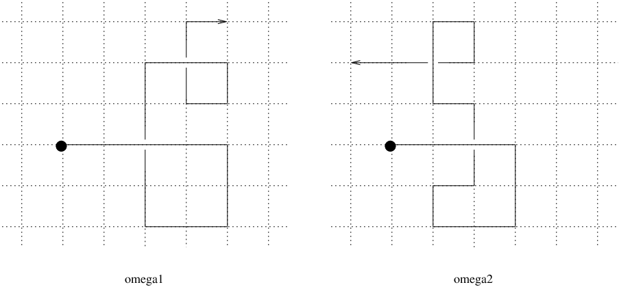
This coarse grained (see Figure 1)

representation of the structure of proteins is often used for numerical studies of protein folding. The very minimalist nature of this representation permits a rapid first search for a protein’s native structure in terms of its contact matrix. In fact, knowledge of the contact matrix can predict many features of the vibrational spectra of certain proteins [1, 5]. This makes it important to have information about the relation between the space of contact matrices and that of the proteins they represent.

To answer the question of how much information about a polymer is retained by its contact matrix, we consider an idealized version of the geometrical structure of a polymer in which the monomers occupy sites on the $n$-dimensional lattice $\mathbb{Z}^{n}$, and consecutive monomers are on nearest neighbor lattice sites.

We compare the Shannon entropy after coarse graining, $S_{C}(N)$, with the Shannon entropy without coarse graining $S(N)$. To quantify the loss of information in the coarse graining we consider $\delta_{N}=S_{C}/S$. We prove, for SRW on $\mathbb{Z}^{2}$, that $\delta_{N}$ goes to one as $N$ becomes large, showing that the relative loss of information $(S-S_{C})/S$ vanishes. This is a consequence of the recurrence of SRW on $\mathbb{Z}^{2}$. Moreover we provide some bounds on finite size corrections (see (3.1b)). On the other hand, for SRW in $\mathbb{Z}^{n}$, $n\geq 3$, and for SAW in $\mathbb{Z}^{n}$, $n\geq 2$, $\delta_{N}$ remains strictly less than one, which means that the loss of information due to the coarse graining becomes substantial (see (3.2b) and Theorem 3.3).

We also consider the problem addressed already in [14], i.e. how the number of different physical contact matrices $W(N)$ depends on the polymer length $N$. It was shown there analytically that $W(N)$ increases exponentially in $N$, and numerically that the growth exponent $\gamma_{N}$ is strictly less than the growth exponent for the total number of SAW. In our work we give a rigorous proof of this (see Theorem 3.3). We also consider the same problem for SRW. Surprisingly, the growth exponent for the contact matrices is now the same as for the number of SRW in all dimensions. The reason for this is that the probability distribution of the number of distinct visited sites (divided by $N$) has a left tail which does not decay exponentially fast in $N$. To conclude, we provide lower bounds on $\gamma_{N}$, relevant to the finite size behaviour (see (3.1a) and (3.2a)).

The outline of the rest of the paper is as follows. In section 2 we introduce the model, the relevant quantities and the studied examples. The main results are presented and briefly discussed in section 3. Sections 4, 5, and 6 are devoted to the proof of the main results.

We define more precisely the quantities and the examples which will be studied. $\Omega_{N}$ is the set of all polymers containing $N+1$ monomers, where the configuration of such a polymer is specified by $\omega_{N}=(\omega(0),\omega(1),...,\omega(N))$ with $\omega(0)\equiv 0$ and $\omega(i+1)-\omega(i)=\pm e_{\alpha}$, where $e_{\alpha}$ is one of the unit directions on $\mathbb{Z}^{n}$, $\alpha=1,...,n$. Let there be given some probability distribution $\mathbb{P}(\omega)$ on $\Omega$. (We shall drop the subscript $N$ whenever possible.) The contact matrices $\mathbf{C}=\{{\cal C}(\omega)\}_{\omega\in\Omega}$ partition $\Omega$ into sets $\Omega_{C}=\{\omega:{\cal C}(\omega)=C\}$, with

the number of configurations $\omega\in\Omega_{C}$. The probability of $\omega$ being in $\Omega_{C}$ is then

To measure the information lost in the coarse-graining we may compare the Shannon entropy $S_{C}$ of the coarse grained measure $\mathbb{P}(C)$ with the fine grained entropy $S$,

We then have

where

with

is the conditional probability of $\omega$ given that it is in $\Omega_{C}$. We can thus think of $\hat{S}_{C}$ as the average “conditional entropy” relative to ${\cal C}$. Since $\hat{S}_{C}\geq 0$ we clearly have $S_{C}\leq S$, and $S-S_{C}$ is then a measure of information lost in the coarse graining [2]. The question is how much. In particular we may ask how does

behave as $N\to\infty$.

Before answering this question we note that

where $\bar{S}_{C}$ is the entropy of the distribution $\bar{\mathbb{P}}(C)$ which assigns equal weight to all $C\in\mathbf{C}$, i.e. $\bar{\mathbb{P}}(C)=W(N)^{-1}$, with $W(N)\equiv|{\bf C}|$ the total number of different coarse grained components, i.e. contact matrices. We may then also define

and by (2.8)

The last inequality is obtained by replacing $\mathbb{P}(C)$ by $\bar{\mathbb{P}}(C)$ in (2.4)-(2.6) and using that the corresponding $\hat{S}_{C}$ is positive.

So far everything is completely general. We shall now specialize to the case where all permissible configurations $\omega$, i.e. all those for which $\mathbb{P}(\omega)\neq 0$, have the same probability. Then

where $\mathbb{E}$ is the expectation value with respect to the relevant uniform distribution.

The examples we shall consider here are:

1) The weights are those of simple symmetric random walks (SRW) on $\mathbb{Z}^{n}$, i.e. $|\Omega|=(2n)^{N}$ and $\mathbb{P}(\omega)=(2n)^{-N}$ for all $\omega$.

2) The polymers behave like self avoiding walks (SAW) on $\mathbb{Z}^{n}$, i.e. the configuration space $\Omega$ consists of all $\omega$ s.t. $\omega(i)\neq\omega(j)$ for $i\neq j$, and $\mathbb{P}(\omega)=|\Omega|^{-1}$, where $|\Omega|\sim\mu_{SAW}^{N}$ is the number of SAW on $\mathbb{Z}^{n}$ of length $N$. SAW model the steric exclusion effects of the monomers and are frequently used as a model for polymers [4, 9].

3) The chains behave like bond self avoiding walks (BAW) on $\mathbb{Z}^{n}$ in which case $\Omega$ consists of all $\omega$ such that the pair $[\omega(i),\omega(i+1)]\neq[\omega(j),\omega(j\pm 1)]$ for $i\neq j$, and $\mathbb{P}(\omega)=|\Omega|^{-1}$, $|\Omega|\sim\mu_{BAW}^{N}$, the number of BAW [12].

Note that for uniform distributions $S$ is just the logarithm of the total number of configurations, i.e. $S=\ln|\Omega|$, so $\gamma_{N}$ is just the ratio of the logarithms of the numbers of contact matrices and random walks.

The behavior of $\gamma_{N}$ was studied in [14] for the case of SAW, with

(The inequality can in fact be made an equality here since $1$ is the minimal distance between $\omega(i)$ and $\omega(j)$ for $i\neq j$.) Numerical studies [14] for $n=2$ indicated that $\gamma_{N}$ remains strictly less than $1$ in the limit $N\to\infty$. It is then natural to ask whether the same is true for the SRW when we again define ${\cal C}_{ij}(\omega)=1$ when $\omega(i)$ and $\omega(j)$ are as close as they can be, i.e. when $a$ in (1.1) is set equal to zero

Note that for this case $W(N)$ satisfies

Since for SRW $\gamma_{N}=\frac{\ln W(N)}{N\ln(2n)}$ it follows from (2.14) that $\gamma_{N}$ is monotone non-decreasing in $N$ and thus that $\lim_{N\to\infty}\gamma_{N}$ exists: remember $\gamma_{N}\leq 1$.

In the present work we prove some results about $\delta_{N}$ and $\gamma_{N}$ for all the above examples. (Some of these generalize readily to other uniform distributions.)

We are indebted to Harry Kesten for the key idea in the proof of Theorem 3.3 for SAW. The extension to BAW is straightforward.

Intuitively we expect that the larger the number of intersections, the more information is contained in the contact matrices. It is therefore not surprising that for recurrent RW, such as SRW in $n=2$, both $\gamma_{N}$ and $\delta_{N}$ would go to $1$. (For the degenerate case $n=1$ there are, for all the cases, just twice as many random walks as contact matrices corresponding to whether the first step is to the right or the left.) One expects however that for RW which have a strong tendency to spread out such as SAW in $n\geq 2$, and SRW in $n\geq 3$ the contact matrices lose too much information. This is indeed reflected in $\delta_{N}<1$ for SAW in $n\geq 2$, and SRW in $n\geq 3$. The same is true for $\gamma_{N}$ for SAW. Surprisingly however $\gamma_{N}\to 1$ for SRW in all dimensions. The reason for this, as we shall see, is that the probability that an SRW of length $N$ in $\mathbb{Z}^{n}$ visits $R_{N}\leq\epsilon N$ distinct sites goes to zero slower than exponentially when $N\to\infty$ for any fixed $\epsilon>0$.

The outline of the rest of the paper is as follows. In section 4 we first present some general inequalities and then prove the results about $\gamma_{N}$ for SRW. In section 5 we give some bounds on the degeneracy of SRW and then prove the results about $\delta_{N}$ for SRW. In section 6 we prove Theorem 3.3 for SAW and BAW.

Using Jensen’s inequality on the average over $\Omega_{C}$, gives

Writing now

we obtain¹¹ 1 The right side of (4.3) is the maximum of the entropy over all measures, $\mu(\omega)$ such that $\mu({\cal C})=\mathbb{P}({\cal C})$.

which yields

We next give an upper bound for the degeneracy of the contact matrices defined in (2.13). This is the key to our results for SRW. Note that for the examples considered here, the first inequality in (4.4) is indeed an equality.

Define the range $R_{N}$ of a SRW with length $N$ to be the number of distinct sites visited by the walk.

There exists also an upper bound on $\gamma_{N}$ which depends on the decrease of $\mathbb{P}(R_{N}/N<\varepsilon)$.

The contact matrix of $\omega$ is now defined by (2.12).

Let us consider the case of SAW. We introduce some notation: we consider a cube $D=\{x\in\mathbb{Z}^{n}\textrm{ s.t. }c_{i}\leq x^{(i)}\leq c_{i}+b,1\leq i\leq n\}$ for some $c=(c_{1},\ldots,c_{n})\in\mathbb{Z}^{n}$ with its boundary $\partial{D}=\{x\in\mathbb{Z}^{n}\textrm{ s.t. }x^{(i)}=c_{i}+b\textrm{ or }x^{(i)}=c_{i},1\leq i\leq n\}$. A path $P$ is a SAW of finite length, say $k$, starting at the origin, i.e. $P=\{X_{i}(P),0\leq i\leq k\}$ with $X_{0}(P)=0$.

We consider only paths such that there exists a cube $D$ with $X_{0}(P)=0$ and $X_{k}(P)$ two of its vertices and $X_{j}(P)\in D$ for all $0\leq j\leq k$. We say that $(P,D)$ occurs at the $r^{th}$ step $\omega$ if
1. $X_{r+j}(\omega)-X_{r}(\omega)=X_{j}(P)$ for all $j=0,\ldots,k$ and
2. $\omega$ does not occupy any other points of $D$.
$\chi_{N}(j,(P,D))$ is the number of $\omega\in\Omega_{N}$ such that $(P,D)$ occurs at most at $j$ steps.

It is known that $|\Omega_{N}|\simeq\mu_{SAW}^{N}$ with $\mu_{SAW}>0$.

References

• [1] I. Bahar, A.R. Atilgan, and B. Erman, Folding Des. 2, 173 (1997).
• [2] P. Billingsley, Ergodic Theory and Information, New York, Wiley ed. (1965).
• [3] P.L. Ferrari, Contact matrices for random walks, EPFL-Lausanne diploma thesis.
• [4] K.F. Freed, Polymers as self-avoiding walks, Ann. Probab. 9, 837–556 (1981).
• [5] T. Haliloglu, I. Bahar, and B. Erman, Gaussian Dynamics of Folded Proteins, Phys. Rev. Lett. 79, 3090–3093 (1997).
• [6] Y. Hamana and H. Kesten, A large deviation result for the range of random walk and for the Wiener sausage, Probab. Theory Relat. Fields, 120 (2), 183–208 (2001).
• [7] T.F. Havel, G.M. Crippen, and I.D. Kuntz, Biopolymers, 18, 73 (1979).
• [8] H. Kesten, On the Number of Self-Avoiding Walks, J. Math. Phys. 4, 960 (1963).
• [9] K.F. Lau and K.A. Dill, Macromolecules 22, 3986 (1989).
• [10] J.-F. Le Gall, Commun. Math. Phys. 104, 471–507 (1986); J.-F. Le Gall, Commun. Math. Phys. 104, 509–528 (1986).
• [11] S. Lifson and C. Sander, Nature (London), 282, 109 (1979).
• [12] N. Madras and G. Slade, The Self-Avoiding Walk, Probability and Its Applications, Birkäuser Boston ed. (1996).
• [13] Th. M. Nieuwenhuizen, Trapping and Lifshitz Tails in Random Media, Self-Attracting Polymers and the Number of Distinct Sites Visited: A Renormalized Instanton Approach in Three Dimensions, Phys. Rev. Lett. 62 (4), 357–360 (1989).
• [14] M. Vendruscolo, B. Subramanian, I. Kanter, E. Domany, and J.L. Lebowitz, Statistical Properties of Contact Maps, Phys. Rev. E, 59, 977–984 (1999).
• [15] M. Vendruscolo, E. Kussell, and E. Domany, Folding Des. 2, 295 (1997).
• [16] F. van Wijland, S. Caser, and H.J. Hilhorst, Topology of the support of the two-dimensional random walk, J. Phys. A 30, 507 (1997).
• [17] F. van Wijland and H.J. Hilhorst, Universal Fluctuations in the Support of the Random Walk, J. Stat. Phys. 89, 119 (1997).
• [18] F. van Wijland, Thèse, Université de Paris-Sud, U.F.R. Scientifique d’Orsay (1998).