Analytical calculation of the solid angle defined by a cylindrical detector and a point cosine source with orthogonal axes

M. J. Prata Email: mjprata@sapo.pt Address: Instituto Tecnológico e Nuclear (ITN), Sacavém, Portugal Thanks: Supported by Fundação para a Ciência e Tecnologia (Programa Praxis XXI - BD/15808/98)

Abstract

We derive analytical expressions for the solid angle subtended by a right circular cylinder at a point source with cosine angular distribution in the case where the source and the cylinder axes are mutually orthogonal.

Keywords:

solid angle, point cosine source, cylindrical detector, cylinder

1 Introduction

The calculation of the solid angle subtended by a cylindrical detector at a point source is of common interest in nuclear science. The case of an isotropic source has been extensively studied, but, to the best of our knowledge, no work has been published considering a point cosine source. Such source could arise as the second term in a Legendre expansion of a general source or, to take a well known example, as one of the terms in the Fermi expression $\ \Phi(\mu)=1+\sqrt{3}\mu$ . This expression holds for the angular distribution of low energy neutrons leaking from a variety of scattering materials and, if suitably modified ( $\Phi(\mu)=1+A\mu$ ), can also be used in the case of lithium hydride (Verbinski, 1967). The scattering of neutrons from hydrogen nuclei considered at rest is also described by a cosine distribution (Ott, 1989).

In this work the situation of a point cosine source defined with respect to some axis and a right circular cylinder with axis orthogonal to that of the source is considered. Under this restriction we present the analytical calculation of the solid angle subtended at the source positioned at an arbitrary location. Sample graphics of the expressions obtained are presented.

2 Solid Angle Calculation

Let the unit vector $\mathbf{k}$ define the source direction. The source distribution $f(\mathbf{\Omega})$ giving the probability $f(\mathbf{\Omega})d\Omega$ of emission around the direction of the unit vector $\mathbf{\Omega}$ is defined by

f(\mathbf{\Omega})=\left\{\begin{array}[c]{cc}\frac{\mathbf{k}\cdot\mathbf{\Omega}}{\pi}&,\mathbf{k}\cdot\mathbf{\Omega\geq 0}\\ 0&,\mathbf{k}\cdot\mathbf{\Omega<0}\end{array}\right.~.

(1)

The distribution is normalized so that

\iint\limits_{all\,directions}f(\mathbf{\Omega})d\Omega=1~.

(2)

The solid angle ( $\Omega$ ) is given by

\Omega=\iint\limits_{\begin{subarray}{c}directions\\ hitting\,detector\end{subarray}}f(\mathbf{\Omega})d\Omega~.

(3)

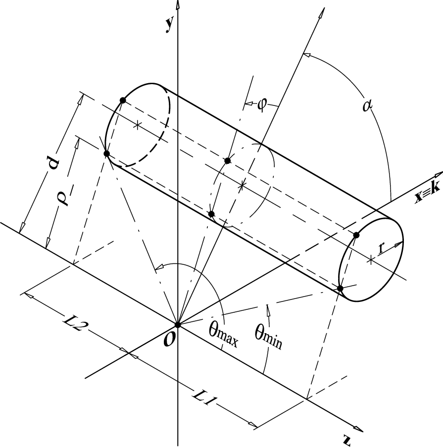
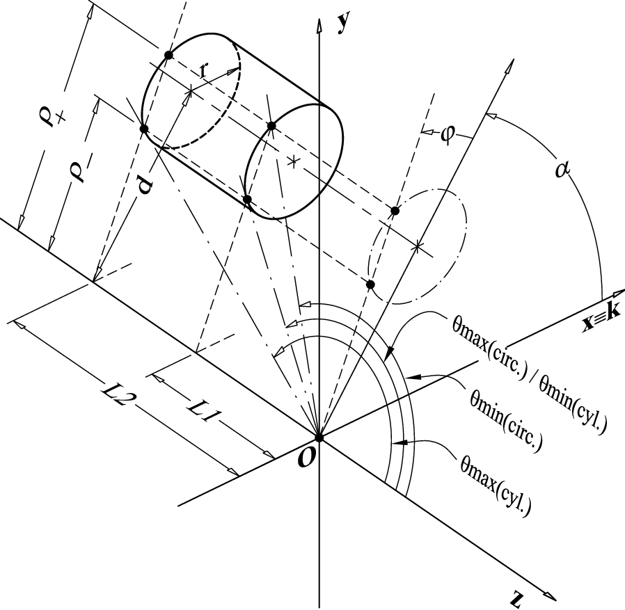
The origin of the coordinate system is chosen to coincide with the point source, the $x$ axis aligned with $\mathbf{k}$ and the $z$ axis parallel to the cylinder axis. In figs. 1 to 3 we show the three cases to be considered and introduce some of the notation used. Generally the solid angle is a sum of two terms, the one subtended by the cylindrical surface ( $\Omega_{cyl}$ ) and the other by either of the end circles ( $\Omega_{circ}$ ). In case (i) one has $\Omega\equiv\Omega_{cyl}$ , in case (ii) $\Omega\equiv\Omega_{cyl}+\Omega_{circ}$ and in case (iii), $\Omega\equiv\Omega_{circ}$ . In the various cases $L_{1}$ , $L_{2}$ , $d$ and $r$ are all positive. From the symmetry of the problem, the solid angle is an even function of $\alpha$ and in the following we will thus consider $\alpha\geq 0$ . In cases (i) and (ii) one has $d\geq r$ and, in case (iii), $r>d$ . With the notation used there results that

\mathbf{k}\cdot\mathbf{\Omega}=\cos(\alpha+\varphi)\sin(\theta)

(4)

where $\theta$ is the polar angle from the z axis and $\varphi$ is the azimuthal angle in the $xy$ plane as measured from an axis through the origin and intersecting the detector axis. Hence

\Omega=\frac{1}{\pi}\int\limits_{\varphi_{\min}}^{\varphi_{\max}}\int\limits_{\theta_{\min}}^{\theta_{\max}}\cos(\alpha+\varphi)\sin^{2}(\theta)d\theta d\varphi

(5)

where the limiting angles have yet to be determined.

Refer to caption — Figure 1: Geometry in Case (i)

2.1 Integration limits

Because the source only emits into the hemisphere corresponding to $x\geq 0$ , the range of variation of $\varphi$ depends on the value of $\alpha$ , as explained in figs. 4 to 7, where the the hashed area shows the illuminated part of the detector. Introducing

\varphi_{0}=\arcsin\left(r/d\right)~,

(6)

there results

\alpha_{1}=\pi/2-\varphi_{0}

(7)

and

\alpha_{c}=\pi/2+\varphi_{0}~.

(8)

The limits for $\varphi$ are then given in table 1.

Table 1: Integration limits for

\varphi

Case	$\alpha\,$ range	$\varphi_{\min}$	$\varphi_{\max}$
	$0\leq\alpha<\alpha_{1}$	$-\varphi_{0}$	$\varphi_{0}$
(i) or (ii)	$\alpha_{1}\leq\alpha<\alpha_{c}$	$-\varphi_{0}$	$\pi/2-\alpha$
	$\alpha_{c}\leq\alpha\leq\pi$	$\Omega=0$
(iii)	$0\leq\alpha\leq\pi$	$-\pi/2-\alpha$	$\pi/2-\alpha$

The limits for $\theta$ can be expressed in terms of $\rho_{{}_{-}}(\varphi)$ and $\rho_{+}(\varphi)$ that were introduced in the pictures and are given by

\rho\pm(\varphi)=d\cos(\varphi)\pm\sqrt{r^{2}-(d\sin(\varphi))^{2}}~.

(9)

The limits for $\theta$ are summarized in table 2.

Table 2: Integration limits for

\theta

Case	$\Omega_{cyl}$ or $\Omega_{circ}$	$\theta_{\min}$	$\theta_{\max}$
(i)	$\Omega_{cyl}$	$\pi/2-\arctan(\frac{L_{1}}{\rho_{-}})$	$\pi/2+\arctan(\frac{L_{2}}{\rho_{-}})$
(ii)	$\Omega_{cyl}$	$\pi/2+\arctan(\frac{L_{1}}{\rho_{-}})$	$\pi/2+\arctan(\frac{L_{2}}{\rho_{-}})$
(ii)	$\Omega_{circ}$	$\pi/2+\arctan(\frac{L_{1}}{\rho_{+}})$	$\pi/2+\arctan(\frac{L_{1}}{\rho_{-}})$
(iii)	$\Omega_{circ}$	$\pi/2+\arctan(\frac{L_{1}}{\rho_{+}})$	$\pi$

2.2 Integration

Let us define

f_{1}(L,d,r,\alpha,\varphi)\equiv f_{1}(\varphi)=\frac{1}{2\pi}\int\cos(\alpha+\varphi)\left[\arctan\left(\frac{L}{\rho_{{}_{-}}}\right)+\frac{L\,\rho_{{}_{-}}}{L^{2}+\rho_{{}_{-}}^{2}}\right]d\varphi

(10)

and

f_{2}(L,d,r,\alpha,\varphi)\equiv f_{2}(\varphi)=\frac{1}{2\pi}\int\cos(\alpha+\varphi)\left[\arctan\left(\frac{L}{\rho_{+}}\right)+\frac{L\,\rho_{+}}{L^{2}+\rho_{{}_{+}}^{2}}\right]d\varphi

(11)

Then, performing the first integration in the rhs of eq. 5, where $\theta_{\min}$ and $\theta_{\max}$ are given in table 2, yields in each case:

case (i)

\Omega=\Omega_{cyl}=\left[f_{1}(L_{1},d,r,\alpha,\varphi)+f_{1}(L_{2},d,r,\alpha,\varphi)\right]_{\varphi_{\min}}^{\varphi_{\max}}~,

(12)

case (ii)

\Omega_{cyl}=\left[f_{1}(L_{2},d,r,\alpha,\varphi)-f_{1}(L_{1},d,r,\alpha,\varphi)\right]_{\varphi_{\min}}^{\varphi_{\max}}~,

(13)

\Omega_{circ}=\left[f_{1}(L_{1},d,r,\alpha,\varphi)-f_{2}(L_{1},d,r,\alpha,\varphi)\right]_{\varphi_{\min}}^{\varphi_{\max}}~,

(14)

\Omega=\Omega_{cyl}+\Omega_{circ}=\left[f_{1}(L_{2},d,r,\alpha,\varphi)-f_{2}(L_{1},d,r,\alpha,\varphi)\right]_{\varphi_{\min}}^{\varphi_{\max}}~,

(15)

case (iii)

	$\displaystyle\Omega$	$\displaystyle=\Omega_{circ}=\frac{1}{4}\int_{\varphi_{\min}}^{\varphi_{\max}}\mathbf{\cos}(\alpha+\varphi)d\varphi-f_{2}(L_{1},d,r,\alpha,\varphi)\|_{\varphi_{\min}}^{\varphi_{\max}}~,$		(16)
		$\displaystyle=\frac{1}{2}-f_{2}(L_{1},d,r,\alpha,\varphi)\|_{\varphi_{\min}}^{\varphi_{\max}}~.$		(17)

Eq. 17 is obtained from eq. 16 by integration of the 1st term using the values from table 1.

Using again the limits from table 1, eqs. 12 to 15 and 17 can be rewritten as

case (i)

\Omega=\Omega_{cyl}=F_{1}(L_{1},d,r,\alpha)+F_{1}(L_{2},d,r,\alpha)~,

(18)

case (ii)

\Omega_{cyl}=F_{1}(L_{2},d,r,\alpha)-F_{1}(L_{1},d,r,\alpha)~,

(19)

\Omega_{circ}=F_{1}(L_{1},d,r,\alpha)-F_{2}(L_{1},d,r,\alpha)~,

(20)

\Omega=\Omega_{cyl}+\Omega_{circ}=F_{1}(L_{2},d,r,\alpha)-F_{2}(L_{1},d,r,\alpha)~,

(21)

case (iii)

\Omega=\Omega_{circ}=F_{3}(L_{1},d,r,\alpha)~,

(22)

where the integrals $F_{i}\;(i=1..3)$ are defined in table 3.

Table 3: Definition of the integrals

F_{i}

Integral	$\alpha\,$ range	Value	$\varphi_{\min}$	$\varphi_{\max}$
	$0\leq\alpha<\alpha_{1}$	$f_{i}(L,d,r,\alpha,\varphi)\|_{\varphi_{\min}}^{\varphi_{\max}}$	$-\varphi_{0}$	$\varphi_{0}$
$F_{i}$ $(i=1,2)$	$\alpha_{1}\leq\alpha<\alpha_{c}$	$f_{i}(L,d,r,\alpha,\varphi)\|_{\varphi_{\min}}^{\varphi_{\max}}$	$-\varphi_{0}$	$\pi/2-\alpha$
	$\alpha_{c}\leq\alpha\leq\pi$	$0$	-	-
$F_{3}$	$0\leq\alpha\leq\pi$	$1/2-f_{2}(L,d,r,\alpha,\varphi)\|_{\varphi_{\min}}^{\varphi_{\max}}$	$-\pi/2-\alpha$	$\pi/2-\alpha$

2.2.1 Calculation of $F_{1}$

Integrating by parts the 1st term in the rhs of eq. 10,

	$\displaystyle\int\cos(\alpha+\varphi)\arctan\left(\frac{L}{\rho_{{}_{-}}}\right)d\varphi=\sin(\alpha+\varphi)\arctan\left(\frac{L}{\rho_{{}_{-}}}\right)$
	$\displaystyle+\int\sin(\alpha+\varphi)\frac{L}{L^{2}+\rho_{{}_{-}}^{2}}\frac{d\sin(\varphi)\rho_{{}_{-}}}{\sqrt{r^{2}-\left[d\sin(\varphi)\right]^{2}}}d\varphi$		(23)

Substituting eq. 23 in the rhs of eq. 10 yields, after some algebra,

f_{1}(\varphi)=\frac{1}{2\pi}\left[A_{10}+\cos(\alpha)A_{11}+\sin(\alpha)A_{12}\right]~,

(24)

where

A_{10}=\sin(\alpha+\varphi)\arctan\left(\frac{L}{\rho_{{}_{-}}}\right)~,

(25)

A_{11}=\int\frac{L\rho_{{}_{-}}}{L^{2}+\rho_{{}_{-}}^{2}}\left(\cos(\varphi)+\frac{d\sin^{2}(\varphi)}{\sqrt{r^{2}-\left[d\sin(\varphi)\right]^{2}}}\right)d\varphi

(26)

and

A_{12}=\int\frac{L\rho_{{}_{-}}}{L^{2}+\rho_{{}_{-}}^{2}}\left(\frac{\rho_{{}_{-}}\sin(\varphi)}{\sqrt{r^{2}-\left[d\sin(\varphi)\right]^{2}}}\right)d\varphi~.

(27)

Performing a change of integration variable to $\phi_{-}$ represented in fig. 8,

\phi_{-}=2\arctan\left(\frac{\rho_{{}_{-}}\sin(\varphi)}{d+r-\rho_{{}_{-}}\cos(\varphi)}\right)~,

(28)

we find

A_{11}=Lr\int\frac{\cos(\phi_{-})}{L^{2}+\rho_{-}^{2}\left(\phi_{-}\right)}d\phi_{-}

(29)

and

A_{12}=Lr\int\frac{\sin(\phi_{-})}{L^{2}+\rho_{-}^{2}\left(\phi_{-}\right)}d\phi_{-}~,

(30)

where

\rho_{{}_{-}}(\phi_{-})=\sqrt{d^{2}+r^{2}-2dr\cos(\phi_{-})}~.

(31)

One then easily obtains

A_{11}=\frac{L}{2d}\left[\frac{2}{\sqrt{1-m^{2}}}\arctan\left(\sqrt{\frac{1+m}{1-m}}\tan\left(\frac{\phi_{-}}{2}\right)\right)-\phi_{-}\right]~,

(32)

where

m=\frac{2dr}{L^{2}+d^{2}+r^{2}}\;\;;~0<m<1

(33)

and

A_{12}=\frac{L}{2d}\log(L^{2}+\rho_{{}_{-}}^{2})~.

(34)

2.2.2 Evaluation of $F_{1}$ ( $d\neq r$ )

For $0\leq\alpha<\alpha_{1}$ the terms proportional to $\sin(\alpha)$ vanish and one gets

	$\displaystyle F_{1}(L,d,r,\alpha)=\frac{\cos(\alpha)}{\pi}\left[\frac{r}{d}\arctan\left(\frac{L}{\sqrt{d^{2}-r^{2}}}\right)\right.$
	$\displaystyle\left.+\frac{L}{d}\left(\frac{1}{\sqrt{1-m^{2}}}\arctan\left(\sqrt{\frac{1+m}{1-m}}\sqrt{\frac{d-r}{d+r}}\right)-\arctan\left(\sqrt{\frac{d-r}{d+r}}\right)\right)\right].$		(35)

For $\ \alpha_{1}\leq\alpha<\alpha_{c}$ , the expressions are less simple and we give each term in eq. 24 separately. Setting

	$\displaystyle\widetilde{\rho}_{-}$	$\displaystyle=\rho_{-}(\varphi_{\max})=\rho_{{}_{-}}\|_{\varphi=\pi/2-\alpha}$		(36)
		$\displaystyle=d\sin\left(\alpha\right)-\sqrt{r^{2}-\left[d\cos\left(\alpha\right)\right]^{2}}~,$		(37)

the first term can be written as

A_{10}|_{\varphi_{\min}}^{\varphi_{\max}}=\arctan\left(\frac{L}{\widetilde{\rho}_{-}}\right)-\arctan\left(\frac{L}{\sqrt{d^{2}-r^{2}}}\right)\sin(\alpha-\varphi_{0})~.

(38)

Defining

a_{1}=\tan\left[\frac{\phi_{-}}{2}\right]_{\varphi_{\min}}=-\sqrt{\frac{d-r}{d+r}}

(39)

and

b_{1}=\tan\left[\frac{\phi_{-}}{2}\right]_{\varphi_{\max}}=\frac{\cos\left(\alpha\right)\widetilde{\rho}_{-}}{r+d-\sin\left(\alpha\right)\widetilde{\rho}_{-}}~,

(40)

then

	$\displaystyle A_{11}\|_{\varphi_{\min}}^{\varphi_{\max}}=\frac{L}{2d}\left\{\frac{2}{\sqrt{1-m^{2}}}\left[\arctan\left(\sqrt{\frac{1+m}{1-m}}b_{1}\right)-\arctan\left(\sqrt{\frac{1+m}{1-m}}a_{1}\right)\right]\right.$
	$\displaystyle\left.-2\left[\arctan\left(b_{1}\right)-\arctan\left(a_{1}\right)\right]\right\}$		(41)

Finally, from $A_{12}$ results

A_{12}|_{\varphi_{\min}}^{\varphi_{\max}}=\frac{L}{2d}\log[\frac{L^{2}+\widetilde{\rho}_{-}^{2}}{L^{2}+d^{2}-r^{2}}]~.

(42)

Using eqs. 24, 38, 41 and 42, $F_{1}$ can be calculated in the case $\alpha_{1}\leq\alpha<\alpha_{c}$ , $d\neq r$ .

2.2.3 Evaluation of $F_{1}$ ( $d=r$ )

The value of $F_{1}$ when $d=r$ can be obtained from eq. 10 using the integration limits from table 3 or calculating the limit of the expressions obtained in 2.2.2, for $\alpha\geqslant\alpha_{1}$ . When $L\neq 0$ one obtains $F_{1}(L,r,r,\alpha)=(1+\cos\alpha)/4$ . Since $F_{1}=0$ for $L=0$ , $F_{1}$ is discontinuous when $r=d$ , $L\rightarrow 0$ .

2.2.4 Calculation of $F_{2}$

The calculation is very similar to that of $F_{1}$ . Integration by parts gives

	$\displaystyle\int\cos(\alpha+\varphi)\arctan\left(\frac{L}{\rho_{+}}\right)d\varphi=\sin(\alpha+\varphi)\arctan\left(\frac{L}{\rho_{+}}\right)$
	$\displaystyle-\int\sin(\alpha+\varphi)\frac{L}{L^{2}+\rho_{+}^{2}}\frac{d\sin(\varphi)\rho_{+}}{\sqrt{r^{2}-\left[d\sin(\varphi)\right]^{2}}}d\varphi~.$		(43)

Eq. 11 can then be rewritten as

f2(\varphi)=\frac{1}{2\pi}\left[A_{20}+\cos(\alpha)A_{21}+\sin(\alpha)A_{22}\right]~,

(44)

where

A_{20}=\sin(\alpha+\varphi)\arctan\left(\frac{L}{\rho_{+}}\right)~,

(45)

A_{21}=\int\frac{L\rho_{+}}{L^{2}+\rho_{+}^{2}}\left(\cos(\varphi)-\frac{d\sin^{2}(\varphi)}{\sqrt{r^{2}-\left[d\sin(\varphi)\right]^{2}}}\right)d\varphi

(46)

and

A_{22}=-\int\frac{L\rho_{+}}{L^{2}+\rho_{+}^{2}}\left(\frac{\rho_{+}\sin(\varphi)}{\sqrt{r^{2}-\left[d\sin(\varphi)\right]^{2}}}\right)d\varphi~.

(47)

The integration variable is now changed to $\phi_{+}$ (fig. 8)

\phi_{+}=2\arctan\left(\frac{\rho_{+}\sin(\varphi)}{r-d+\rho_{+}\cos(\varphi)}\right)

(48)

and the integrals are then expressed as

A_{21}=Lr\int\frac{\cos(\phi_{+})}{L^{2}+\rho_{+}^{2}\left(\phi_{+}\right)}d\phi_{+}~,

(49)

A_{22}=-Lr\int\frac{\sin(\phi_{+})}{L^{2}+\rho_{+}^{2}\left(\phi_{+}\right)}d\phi_{+}~,

(50)

where

\rho_{+}(\phi_{+})=\sqrt{d^{2}+r^{2}+2dr\cos(\phi_{+})}~.

(51)

The integration is straightforward resulting in

A_{21}=\frac{L}{2d}\left[\phi_{+}-\frac{2}{\sqrt{1-m^{2}}}\arctan\left(\sqrt{\frac{1-m}{1+m}}\tan\left(\frac{\phi_{+}}{2}\right)\right)\right]

(52)

and

A_{22}=\frac{L}{2d}\log(L^{2}+\rho_{+}^{2})~.

(53)

where $m$ is obtained from eq. 33.

2.2.5 Evaluation of $F_{2}$ ( $d\neq r$ )

For $0\leq\alpha<\alpha_{1}$ the terms proportional to $\sin(\alpha)$ again vanish giving

	$\displaystyle F_{2}(L,d,r,\alpha)=\frac{\cos(\alpha)}{\pi}\left[\frac{r}{d}\arctan\left(\frac{L}{\sqrt{d^{2}-r^{2}}}\right)\right.$
	$\displaystyle\left.-\frac{L}{d}\left(\frac{1}{\sqrt{1-m^{2}}}\arctan\left(\sqrt{\frac{1-m}{1+m}}\sqrt{\frac{d+r}{d-r}}\right)-\arctan\left(\sqrt{\frac{d+r}{d-r}}\right)\right)\right]~.$		(54)

It is interesting that using $\arctan(z)+\arctan(1/z)=\pi/2$ the expression can be recast as

F_{2}(L,d,r,\alpha)=F_{1}(L,d,r,\alpha)+\cos(\alpha)\,L/(2d)\,\left(1-1/\sqrt{1-m^{2}}\right)~.

(55)

For $\ \alpha_{1}\leq\alpha<\alpha_{c}$ , setting

	$\displaystyle\widetilde{\rho}_{+}$	$\displaystyle=\rho_{+}(\varphi_{\max})=\rho_{+}\|_{\varphi=\pi/2-\alpha}$		(56)
		$\displaystyle=d\sin\left(\alpha\right)+\sqrt{r^{2}-\left(d\cos\left(\alpha\right)\right)^{2}}~,$		(57)

the first term is determined from

A_{20}|_{\varphi_{\min}}^{\varphi_{\max}}=\arctan\left(\frac{L}{\widetilde{\rho}_{+}}\right)-\arctan\left(\frac{L}{\sqrt{d^{2}-r^{2}}}\right)\sin(\alpha-\varphi_{0})~.

(58)

Considering

	$\displaystyle a_{2}$	$\displaystyle=\tan\left[\frac{\phi_{+}}{2}\right]_{\varphi_{\min}}=-\sqrt{\frac{d+r}{d-r}}~,$		(59)
	$\displaystyle b_{2}$	$\displaystyle=\tan\left[\frac{\phi_{+}}{2}\right]_{\varphi_{\max}}=\frac{\cos\left(\alpha\right)\widetilde{\rho}_{+}}{r-d+\sin\left(\alpha\right)\widetilde{\rho}_{+}}~,$		(60)

gives

	$\displaystyle A_{21}\|_{\varphi_{\min}}^{\varphi_{\max}}=\frac{L}{2d}\left\{2\left[\arctan\left(b_{2}\right)-\arctan\left(a_{2}\right)\right]\right.$
	$\displaystyle\left.-\frac{2}{\sqrt{1-m^{2}}}\left[\arctan\left(\sqrt{\frac{1-m}{1+m}}b_{2}\right)-\arctan\left(\sqrt{\frac{1-m}{1+m}}a_{2}\right)\right]\right\}~.$		(61)

Finally, for $A_{22}$ the result is

A_{22}|_{\varphi_{\min}}^{\varphi_{\max}}=\frac{L}{2d}\log[\frac{L^{2}+\widetilde{\rho}_{+}^{2}}{L^{2}+d^{2}-r^{2}}]~,

(62)

which completes the evaluation of $F_{2}$ when $r\neq d$ .

2.2.6 Evaluation of $F_{2}$ ( $d=r$ )

Taking the limit of the expressions obtained in 2.2.5 when $L\neq 0$ , one obtains $F_{2}(L,r,r,\alpha=0)=1/2+L/(2r)(1-1/\sqrt{1-m^{2}})$ , $F_{2}(L,r,r,\alpha=\pi)=0$ and

	$\displaystyle F_{2}(L,r,r,\alpha)=(1+\cos\alpha)/4-1/(2\pi)\{\arctan\left[2(r/L)\sin\alpha\right]$
	$\displaystyle+\cos(\alpha)L/r\left(\alpha-\pi+1/\sqrt{1-m^{2}}\left(\pi/2+\arctan\left[\cot(\alpha)\sqrt{1-m}/\sqrt{1+m}\right]\right)\right)$
	$\displaystyle-\sin(\alpha)L/(2r)\log\left[1+4r^{2}\sin^{2}(\alpha)/L^{2}\right]\}~.$		(63)

for $sin(\alpha)\neq 0$ . A simple calculation shows that when $L\rightarrow 0$ , $F_{2}(L,r,r,\alpha)\rightarrow 0$ , regardless of $\alpha$ This is also true when $d\neq r$ , and $F_{2}$ is thus continuous when $L\rightarrow 0$ .

2.2.7 Calculation of $F_{3}$

From table 3,

F_{3}(L,d,r,\alpha)=1/2-f_{2}(L,d,r,\alpha,\varphi)|_{\varphi_{\min}}^{\varphi_{\max}}~.

(64)

The calculation of $f_{2}$ has already been done although the quantities involved ( $\phi_{+}$ , $\rho_{+}$ ) have a different graphical interpretation as shown in fig. 9. Eqs. 48 and 52 can still be used but some care is required as explained further on. From eqs. 64 and 44 follows that

F_{3}=\frac{1}{2\pi}\left[A_{30}+\cos(\alpha)A_{31}+\sin(\alpha)A_{32}\right]_{\varphi_{\min}}^{\varphi_{\max}}~,

(65)

where

$\displaystyle A_{30}$	$\displaystyle=\varphi-A_{20}~,$	(66)
$\displaystyle A_{31}$	$\displaystyle=-A_{21}~,$	(67)
$\displaystyle A_{32}$	$\displaystyle=-A_{22}$	(68)

and $A_{2i}$ , $(i=1..3)$ are determined from eqs. 45, 52 and 53.

2.2.8 Evaluation of $F_{3}$ ( $d\neq 0$ )

With $\varphi_{\max}$ and $\varphi_{\min}$ chosen from table 1

	$\displaystyle\rho_{+}(\varphi_{\max})$	$\displaystyle=\widetilde{\rho}_{+}~,$		(69)
	$\displaystyle\rho_{+}(\varphi_{\min})$	$\displaystyle=-\widetilde{\rho}_{-}~,$		(70)

where $\widetilde{\rho}_{-}$ and $\widetilde{\rho}_{+}$ are found from eqs. 37 and 57. To calculate $A_{31}|_{\varphi_{\min}}^{\varphi_{\max}}$ the quantities

a_{3}=\tan\left[\frac{\phi_{+}}{2}\right]_{\varphi_{\min}}=\frac{\cos\left(\alpha\right)\widetilde{\rho}_{-}}{r-d+\sin\left(\alpha\right)\widetilde{\rho}_{-}}

(71)

and

b_{3}=\tan\left[\frac{\phi_{+}}{2}\right]_{\varphi_{\max}}=\frac{\cos\left(\alpha\right)\widetilde{\rho}_{+}}{r-d+\sin\left(\alpha\right)\widetilde{\rho}_{+}}

(72)

will be useful. $A_{30}$ is given by

A_{30}|_{\varphi_{\min}}^{\varphi_{\max}}=\pi-\left[\arctan\left(L/\widetilde{\rho}_{+}\right)-\arctan\left(L/\widetilde{\rho}_{-}\right)\right]~.

(73)

Using eq. 90 from the appendix results in

A_{30}|_{\varphi_{\min}}^{\varphi_{\max}}=\pi-2\arctan\left(1/z\right)~,

(74)

where

z=\frac{r^{2}-d^{2}-L^{2}+\sqrt{\left(r^{2}-d^{2}-L^{2}\right)^{2}+4L^{2}(r^{2}-\left[d\cos(\alpha)\right]^{2})}}{2L\sqrt{r^{2}-\left[d\cos(\alpha)\right]^{2}}}~.

(75)

Then, applying $\arctan\left(z\right)+\arctan\left(1/z\right)=\pi/2$ yields

A_{30}|_{\varphi_{\min}}^{\varphi_{\max}}=2\arctan\left(z\right)~.

(76)

Some care is required to obtain $A_{31}$ . From fig. 9 is clear that as $\alpha\rightarrow$ $\pi/2$ then $\phi_{+}\left(\varphi_{\min}\right)$ $\rightarrow-\pi$ and that $-\pi<\phi_{+}\left(\varphi_{\min}\right)<-3\pi/2$ for $\alpha>$ $\pi/2$ . Therefore $a_{3}=\tan\left[\phi_{+}(\varphi_{\min})/2\right]$ is not continuous as $\alpha$ goes through $\pi/2$ . The discontinuity also appears in the rhs of eq. 48 when $\varphi$ decreases to less than $-\pi$ . From eqs. 67 and 52 its obvious that both terms in $A_{31}$ will be discontinuous. The integral, of course, must be continuous and a proper expression can be provided by noticing that while

z\neq\arctan\left[\tan(z)\right]\;;-\pi<z<-\pi/2~,

(77)

one has

z=-\pi/2-\arctan\left[1/\tan\left(z\right)\right]\;;-\pi<z<0~.

(78)

Thus, to evaluate $A_{31}$ , the substitutions

\arctan(a_{3})\rightarrow-\pi/2-\arctan(1/a_{3})~,

(79)

\arctan\left(\sqrt{\frac{1-m}{1+m}}a_{3}\right)\rightarrow-\pi/2-\arctan\left[1/\left(\sqrt{\frac{1-m}{1+m}}a_{3}\right)\right]~,

(80)

are used and it is found that

A_{31}|_{\varphi_{\min}}^{\varphi_{\max}}=-\frac{L}{2d}\left\{2\left[\pi/2+\Delta t_{1}\right]-\frac{2}{\sqrt{1-m^{2}}}\left[\pi/2+\Delta t_{2}\right]\right\}~,

(81)

where

\Delta t_{1}=\arctan(b_{3})+\arctan(1/a_{3})~,

(82)

\Delta t_{2}=\arctan(\sqrt{\frac{1-m}{1+m}}b_{3})+\arctan(\sqrt{\frac{1+m}{1-m}}/a_{3})~.

(83)

The sum of arctangents can be cast as a single one using eq. 90 from the appendix and after some algebra one gets

\Delta t_{1}=2\arctan\left[d\cos\left(\alpha\right)/\left(r+E\right)\right]~,

(84)

\Delta t_{2}=2\arctan\left[\left\{Gd\cos\left(\alpha\right)\right\}/\left\{EH+r\sqrt{H^{2}-\left[2Ld\cos\left(\alpha\right)\right]^{2}}\right\}\right]~,

(85)

where

E=\sqrt{r^{2}-\left[d\cos(\alpha)\right]^{2}}~,

(86)

G=L^{2}+d^{2}-r^{2}

(87)

and

H=\sqrt{\left[L^{2}+\left(d+r\right)^{2}\right]\left[L^{2}+\left(d-r\right)^{2}\right]}~.

(88)

The remaining term is given by

A_{32}|_{\varphi_{\min}}^{\varphi_{\max}}=-\frac{L}{2d}\log\left(\frac{L^{2}+\widetilde{\rho}_{+}^{2}}{L^{2}+\widetilde{\rho}_{-}^{2}}\right)~.

(89)

2.2.9 Evaluation of $F_{3}$ ( $d=0$ )

Calculation of the limit of the expressions obtained in 2.2.8 yields $F_{3}(L,d=0,r,\alpha)=1/2-(\arctan\left[L/r\right]+Lr/\left(L^{2}+r^{2}\right))$ . In the same way one can show that $F_{3}(L\rightarrow 0,d<r,r,\alpha)=1/2$ regardless of $d$ , $r$ and $\alpha$ . Altough $F_{3}$ is only needed for $d<r$ , it is worth mentioning that $\underset{L\rightarrow 0}{\lim}(\underset{d\rightarrow r-}{\lim}F_{3}(L,d,r,\alpha))=1/4(1+\cos\alpha)$ .

3 Sample graphics and discussion

To illustrate the behavior with respect to $\alpha$ we consider a cylinder of lenght 10 and radius 1. In figs. 10, 11 and 12 are shown examples of cases (i),(ii) and (iii), respectively. As argued before, $\Omega$ is an even function of $\alpha$ in all cases. In cases (i) and (ii), for $0\leq\left|\alpha\right|<\pi/2-\arcsin(r/d)$ , the solid angle is simply proportional to $cos(\alpha)$ ; for $\left|\alpha\right|>\pi/2+\arcsin(r/d)$ , $\Omega=0$ . In between, the dependence on $\alpha$ is more complicated because a fraction of the cylinder is not illuminated by the source, but $\Omega(\alpha)$ obviously decreases as $\left|\alpha\right|$ increases. The transition region is large for $d\approx r$ ( $d<r$ ) and becomes increasingly narrower as $d$ increases. For $d\gg r$ , the region essentially vanishes so that $\Omega\varpropto cos(\alpha)$ when $\left|\alpha\right|\lessapprox\pi/2$ and $\Omega=0$ when $\left|\alpha\right|\gtrapprox\pi/2$ . It is intuitive that in case (i), $\Omega$ decreases when distance $d$ increases and all other parameters are held constant. This is not necessarily true for case (ii), because source and cylinder are in a skew geometry. Considering two distances $d_{1}<d_{2}$ , one concludes from the preceding discussion that there is certainly some region for $\alpha$ where $\Omega(d_{2})=0$ and $\Omega(d_{1})>0$ so that $\Omega(d_{1})>\Omega(d_{2})$ . As $\left|\alpha\right|$ decreases to $0$ , this relation can be inverted, which happens for all distances shown in fig. 11. Since for very large $d$ , $\Omega$ is certainly a decreasing function of $d$ , there must be a maximum, for each $\alpha.$ This is illustrated in fig. 13, for $\alpha=0$ , $L_{1}=5$ and two cylinder lengths: 10 ( $L_{2}=15$ ) and 20 ( $L_{2}=25$ ). It is worth mentioning that in case (ii), apart form the $\alpha$ dependence, a similar behavior can be observed for an isotropic point source (i.e. a maximum when $d$ is changed and $L_{1}$ and $L_{2}$ kept constant). Case (iii) is exemplified in fig. 12. In this case ( $r>d$ ) the solid angle is defined only by one the end circles which is, in general, partially illuminated by the source. The exception happens when $d\longrightarrow r$ : for $\alpha=0$ the circle is fully illuminated where as for $\alpha=\pi$ it is totally obscured. When $d=0$ the source is aligned with the center of circle and $\Omega$ is then independent of $\alpha$ . As $d$ increases, for $L_{1}\neq 0$ , the dependence on $\alpha$ becomes stronger with a maximum when $\alpha=0$ . When $L_{1}=0$ (not shown in fig. 12), $\Omega=1/2$ , regardless of $\alpha$ or $d$ .

4 Conclusions and outlook

The solid angle defined by a point cosine source and a right circular cylinder with axis orthogonal to that of the source has been treated analitically. It has been shown that for $d>r$ and $0\leqslant\left|\alpha\right|<\pi/2-\arcsin(r/d)$ , the whole dependence on $\alpha$ is given by a $cos(\alpha)$ factor (eqs. 35 and 54). It is possible to obtain, in a similar fashion, analytical expressions in the case of a cosine source distributed on a wire paralell to the cylinder axis. A work where we report these results is in preparation.

I would like to thank João Prata for his thorough review of the manuscript.

Appendix A Sum of Arctans

To prove the identity

\arctan x\pm\arctan y=2\arctan\left[\left(x\pm y\right)/\left(1\mp xy+\sqrt{\left(x\pm y\right)^{2}+\left(1\mp xy\right)^{2}}\right)\right]

(90)

consider $h(x,y)=\arctan x\pm\arctan y$ and $g(x,y)=2\arctan\left[\left(x\pm y\right)/D\right]$ where

D=\left(1\mp xy+\sqrt{\left(x\pm y\right)^{2}+\left(1\mp xy\right)^{2}}\right)~.

Using $\tan(u\pm v)=\left[\tan(u)\pm\tan(v)\right]/\left[1\mp\tan(u)\tan(v)\right]$ , we find that $\tan\left(h\right)=\left(x\pm y\right)/\left(1\mp xy\right)$ . In a similar way, applying $\tan(2u)=2\tan(u)/\left[1-\tan^{2}(u)\right]$ , gives

	$\displaystyle\tan\left[g(x,y)\right]$	$\displaystyle=2\frac{\left(x\pm y\right)/D}{\left[D^{2}-\left(x\pm y\right)^{2}\right]/D^{2}}$
		$\displaystyle=\left(x\pm y\right)/\left(1\mp xy\right)~,$

where in the last step we used the fact that $\ D\neq 0$ . Since $\tan\left(h\right)=\tan\left(g\right)$ then $h-g=n\pi$ for some n. Taking $x=y=0$ results that $n=0$ and, because $h$ and $g$ are continuous, we conclude that eq. 90 holds for any $x$ and $y$ .

References

Ott, (1989) Ott, K.O., Bezella, W.A., 1989. Introductory Nuclear Reactor Statics. American Nuclear Society, La Grange Park, (p.170).
Verbinski, (1967) Verbinski, V.V., 1967. Angular Distributions of Low-Energy Neutrons Leaking from Various Scattering Materials. Nucl. Sci. Eng. 27, 67-69.

Analytical calculation of the solid angle defined by a cylindrical detector and a point cosine source with orthogonal axes

Abstract

Keywords:

1 Introduction

2 Solid Angle Calculation

2.1 Integration limits

2.2 Integration

2.2.1 Calculation of F1F_{1}

2.2.2 Evaluation of F1F_{1} (d≠rd\neq r)

2.2.3 Evaluation of F1F_{1} (d=rd=r)

2.2.4 Calculation of F2F_{2}

2.2.5 Evaluation of F2F_{2} (d≠rd\neq r)

2.2.6 Evaluation of F2F_{2} (d=rd=r)

2.2.7 Calculation of F3F_{3}

2.2.8 Evaluation of F3F_{3} (d≠0d\neq 0)

2.2.9 Evaluation of F3F_{3} (d=0d=0)

3 Sample graphics and discussion

4 Conclusions and outlook

Appendix A Sum of Arctans

References

2.2.1 Calculation of $F_{1}$

2.2.2 Evaluation of $F_{1}$ ( $d\neq r$ )

2.2.3 Evaluation of $F_{1}$ ( $d=r$ )

2.2.4 Calculation of $F_{2}$

2.2.5 Evaluation of $F_{2}$ ( $d\neq r$ )

2.2.6 Evaluation of $F_{2}$ ( $d=r$ )

2.2.7 Calculation of $F_{3}$

2.2.8 Evaluation of $F_{3}$ ( $d\neq 0$ )

2.2.9 Evaluation of $F_{3}$ ( $d=0$ )