Formation of singularities in Yang-Mills equations
Abstract
This is a survey of recent studies of singularity formation in solutions of spherically symmetric Yang-Mills equations in higher dimensions. The main attention is focused on five space dimensions because this case exhibits interesting similarities with Einstein’s equations in the physical dimension, in particular the dynamics at the threshold of singularity formation shares many features (such as universality, self-similarity, and scaling) with critical phenomena in gravitational collapse. The borderline case of four space dimensions is also analyzed and the formation of singularities is shown to be intimately tied to the existence of the instanton solution.
1 Introduction
One of the most interesting features of many nonlinear evolution equations is the spontaneous onset of singularities in solutions starting from perfectly smooth initial data. Such a phenomenon, usually called ”blowup”, has been a subject of intensive studies in many fields ranging from fluid dynamics to general relativity. Whether or not the blowup can occur for a given nonlinear evolution equation is the central mathematical question which, from the physical point of view, has a direct bearing on our understanding of the limits of validity of the corresponding model. Unfortunately, this is often a difficult question. Two famous examples for which the answer is not known are the Navier-Stokes equation and the Einstein equations. Once the existence of blowup is established for a particular equation, many further questions come up, such as: When and where does the blowup occur? What is the character of blowup and is it universal? Can a solution be continued past the singularity?
In this paper we consider these questions for the Yang-Mills (YM) equations in higher dimensions. In the physical dimensions, where the YM equations are the basic equations of gauge theories describing the weak and strong interactions of elementary particles, it is known that no singularities can form. This was shown by Eardley and Moncrief [1] who proved that solutions starting from smooth initial data remain smooth for all future times. The motivation for studying the YM equations in unphysical dimensions for is twofold (and unrelated to the latest fashion of doing physics in extra dimensions). From the mathematical point of view, it is the obvious thing to ask how the property of global regularity depends on the dimension of the underlying spacetime and whether singularities can form in dimensions for . However, there is also a less evident physical reason which is motivated by the hope that by understanding the problem of singularity formation for the YM equations one might get insight into the analogous, but much more difficult, problem in general relativity. From this viewpoint – in which the YM equations are considered as a toy model for the Einstein equations – it is essential that these two equations belong to the same criticality class. Let us recall that the criticality class is defined as the degree in the homogeneous scaling of energy under dilations . The classification of equations into subcritical (), critical (), and supercritical () is a basis of the heuristic meta-principle according to which subcritical equations are globally regular, while supercritical equations may develop singularities for some (large) initial data [2]. For the YM equations we have , while for the Einstein equations . Therefore, the YM equations in have the same criticality, , as the Einstein equations in the physical dimension. Another way of seeing this is to note that in the dimension of the YM coupling constant (in units) is the same as the dimension of the physical Newton’s constant .
For the reason just explained, the main body of this paper is focused on the lowest super-critical dimension . In Section 3 we show that in this case there exists a countable family of regular (by regularity we mean analyticity inside the future light cone) spherically symmetric self-similar solutions labelled by a nonnegative integer (a nodal number). Next, using linear stability analysis we show in Section 4 that the number of unstable modes around a given solution is equal to its nodal number. The role of self-similar solutions in the dynamical evolution is studied in Section 5, where we show that: i) the solution determines a universal asymptotics of singularity formation for solutions starting from generic ”large” initial data; ii) the solution plays the role of a critical solution sitting at the threshold of singularity formation. The latter is in many respects similar to the critical behaviour at the threshold of black hole formation in gravitational collapse. In both cases the threshold of singularity (or black hole) formation can be identified with the codimension-one stable manifold of a self-similar solution with exactly one unstable mode. These similarities are discussed in detail in Section 6.
We consider also the Cauchy problem for the YM equations in . Despite intensive studies of this borderline case, the problem of global existence is open. In Section 7 we describe numerical simulations which, in combination with analytic results, strongly suggest that large-energy solutions do blow up. We show that the process of singularity formation is due to concentration of energy and proceeds via adiabatic shrinking of the instanton solution. At the end, a recent attempt of determining the asymptotic rate of shrinking is sketched.
We remark that there are close parallels between YM equations in dimensions and wave maps in dimensions [3]. Indeed, many of the phenomena described here are mirrored for the equivariant wave maps into spheres in three [4, 5] and two [6] spatial dimensions.
Sections 5 and 7 of this survey are based on joint work with Z. Tabor [7]. The material of Sections 3 and 4 is new.
2 Setup
We consider Yang-Mills (YM) fields in dimensional Minkowski spacetime (in the following Latin and Greek indices take the values and respectively). The gauge potential is a one-form with values in the Lie algebra of a compact Lie group . In terms of the curvature the action is
| (1) |
where is the gauge coupling constant. Hereafter we set . The YM equations derived from (1) are
| (2) |
As written, this equation is underdetermined because of the gauge invariance
| (3) |
where is an arbitrary function with values in . In order to correctly formulate the Cauchy problem for equation (2), one must impose additional conditions which fix this gauge ambiguity. We shall not discuss this issue here because in the spherically symmetric ansatz, to which this paper is restricted, the gauge is fixed automatically.
For simplicity, we take here so the elements of can be considered as skew-symmetric matrices and the Lie bracket is the usual commutator. Assuming the spherically symmetric ansatz [8]
| (4) |
the YM equations reduce to the scalar semilinear wave equation for the magnetic potential
| (5) |
where is the radial Laplacian in dimensions. The central question for equation (5) is: can solutions starting from smooth initial data
| (6) |
become singular in future? As mentioned above, in the physical dimensions Eardley and Moncrief answered this question in the negative [1]. However, simple heuristic arguments indicate that the property of global regularity enjoyed by the YM equations in might break down in higher dimensions. In order to see why the global behaviour of solutions is expected to depend critically on the dimension , we recall two basic facts. The first fact is the conservation of (positive definite) energy
| (7) |
where the coefficient follows from the integration over the angles and taking the trace. The second fact is scale-invariance of the YM equations: if is a solution of (2), so is , or equivalently, if is a solution of (5), so is . Under this scaling the energy scales as , hence the YM equations are subcritical for , critical for , and supercritical for . In the subcritical case, shrinking of solutions to arbitrarily small scales costs infinite amount of energy, so it is forbidden by energy conservation. In other words, transfer of energy to arbitrarily high frequencies is impossible and consequently the Cauchy problem should be well posed in the energy norm. This important fact was proved in by Klainerman and Machedon [9], who thereby strengthened the result of Eardley and Moncrief. In the supercritical case, shrinking of solutions might be energetically favourable and consequently singularities are anticipated. In fact, we shall show below that singularities do form already in the lowest supercritical dimension . In the critical dimension the problem of singularity formation is more subtle because the scaling argument is inconclusive.
3 Self-similar solutions in
In order to set the stage for the discussion of singularity formation we first need to analyze in detail the structure of self-similar solutions of equation (5). As we shall see, these solutions play a key role in understanding the nature of blowup. By definition, self-similar solutions are invariant under dilations , hence they have the form
| (8) |
where a positive constant , clearly allowed by the time translation invariance, is introduced for later convenience. Note that for a self-similar solution we have
| (9) |
hence the solution becomes singular at the center when (there is no blowup in the first derivative because regularity demands that ). Thus, each self-similar solution provides an explicit example of a singularity developing in finite time from smooth initial data.
Substituting the ansatz (8) into (5) one obtains the ordinary differential equation
| (10) |
As explained in the introduction, because of the expected connections with the Einstein equations, we are mainly interested in the lowest super-critical dimension . In this case equation (10) reduces to
| (11) |
Although the similarity coordinate is natural in the discussion of singularity formation, it has a disadvantage of not covering the region , in particular it does not extend to the future light cone of the point . For this reason we define a new coordinate which covers the whole spacetime: the past and the future light cones are located at and , respectively; while the center corresponds to (for ) and (for ). In terms of equation (11) becomes
| (12) |
We first consider this equation inside the past light cone, that is for and impose the boundary conditions
| (13) |
which follow from the demand of smoothness at the endpoints. As we shall see below, once a solution to this boundary value problem is constructed, its extension beyond the past light cone can be easily done.
To show that equation (12) admits solutions satisfying (13) we shall employ a shooting technique. The main idea of this method is to replace the boundary value problem by the initial value problem with initial data imposed at one of the endpoints and then adjusting these data so that the solution hits the desired boundary value at the second endpoint. In the case at hand we shall shoot from towards infinity. Substituting a formal power series expansion about into (12) one finds the asymptotic behaviour
| (14) |
where is a free parameter determining uniquely the whole series. In the following a solution of equation (12) starting at with the asymptotic behaviour (14) will be called an -orbit. Without loss of generality we may assume that . We claim that there is a countable set of values for which the -orbits exist for all and have the desired asymptotics at infinity (such orbits will be called connecting). The proof consists of several steps.
Step 1 (Local existence). First, we need to show that -orbits do in fact exist, that is, the series (14) has a nonzero radius of convergence. Since the point is singular, this fact does not follow from standard theorems. Fortunately, in [10] Breitelohner, Forgács, and Maison have derived the following result concerning the behaviour of solutions of a system of ordinary differential equations near a singular point:
Theorem [BFM]. Consider a system of first order differential equations for functions and
| (15) |
where constants and integers and let be an open subset of such that the functions and are analytic in the neighbourhood of for all . Then there exists an -parameter family of solutions of the system (15) such that
| (16) |
where and are defined for all and are analytic in and .
We shall make use of this theorem to prove the local existence of -orbits. In order to put equation (12) into the form (16) we define the variables
| (17) |
and get
| (18) |
Since the function is analytic near for any and , according to the BFM theorem there exists a one-parameter family of local solutions such that
| (19) |
Transforming (19) back to the original variables we obtain the behaviour of -orbits.
Step 2 (A priori global behaviour). It follows immediately from (12) that for a solution cannot have a maximum (resp. minimum) for (resp. ). Thus, once the solution leaves the strip , it cannot reenter it (actually, such a solution becomes singular for a finite ). It is also clear that as long as the solution cannot go singular. To derive the asymptotics at infinity of -orbits that stay in the strip we shall make use of the following functional
| (20) |
For solutions of equation (12) we have
| (21) |
so is monotone increasing. Now, we shall show that solutions satisfying for all tend to as . To see this, first notice that for such solutions must be negative because if for some then is strictly positive for so the solution must leave the strip in finite time. Since and , it follows that has a nonpositive limit at infinity which in turn implies by (21) that and by (20) that exists. By L’Hôpital’s rule we have and using (12) again, we get that equals or . The latter is impossible because then is a global minimum contradicting the fact that increases. Thus, .
Step 3 (i) (Behaviour of -orbits for small ). Rescaling we get
| (22) |
As , the solutions of this equation tend uniformly on compact intervals to the solution of the limiting equation
| (23) |
with the same initial condition. This equation can be solved explicitly but for the purpose of the argument it suffices to notice that its solution, call it , is oscillating at infinity. Since up to an arbitrarily large if is sufficiently small, it follows that the number of zeros of the solution tends to infinity as .
(ii) (Behaviour of -orbits for large .) We rescale the variables, setting , to get
| (24) |
As , the solutions of this equation tend uniformly on compact intervals to the solution of the limiting equation . Thus, for large and therefore the -orbit crosses for a finite .
Step 4 (Shooting argument). We define the set
| (25) |
We know from Step 3 that the set is nonempty (because the -orbits with large belong to it) and bounded below (because the -orbits with small do not belong to it). Thus exists. The solution cannot cross the line at a finite because the same would be true for nearby solutions, violating the definition of . Thus, for all and hence, by Step 2, . This completes the proof of existence of the nodeless self-similar solution .
Next, let us consider the solution with for small . By the definition of there must be a point where this solution attains a positive local maximum and since no minima are possible for , it follows that there must be a point where . We shall show that provided that is sufficiently small. As argued above this would imply that the solution leaves the strip via . From (21) we have
| (26) |
In order to estimate the last integral note that for
| (27) |
so . Substituting this into (26) one gets
| (28) |
The right hand side of this inequality is equal to for so, by continuity, it remains strictly positive for near . By taking a sufficiently small we can have arbitrarily close to , hence which proves that -orbits with have exactly one zero. This means that the set increases up to some where it attains a positive local maximum and then decreases monotonically up to some where is nonempty. Let . By Step 3, exists and is strictly positive. Using the same argument as above we conclude that the -orbit must stay in the region for all , hence . This completes the proof of existence of the self-similar solution with exactly one zero.
The subsequent connecting orbits are obtained by induction. We conclude that there exists a countable family of self-similar solutions indexed by the integer which counts the number of zeros for .
Remark. Since the sequence is decreasing and bounded below by zero, it has a nonnegative limit . If , then the -orbit cannot leave the region for a finite (because the set of such orbits is clearly open) hence it must be a connecting orbit with some finite number of zeros. But this contradicts the fact that the number of zeros of -orbits increases with . Hence, . This implies that for any finite , goes to zero when .
We remark that the existence of the solution was first shown by Cazenave, Shatah, and Tahvildar-Zadeh [3] via a variational method.
The shooting technique is not only a powerful analytical tool; it is also an efficient numerical method of solving two-point boundary value problems. The numerical results produced by this method are shown in Table 1 and Figure 1.

|
Surprisingly, it turned out that (with very good accuracy). This was a hint that the solution has a simple closed form. Indeed, playing with the power series expansion (14) we found that
| (29) |
Below we show an amusing calculation by Maple which helped us in finding this formula.
restart;
with(DEtools):
with(numapprox):
ode:=(x^2-1)*diff(w(x),x$2)+3*w(x)*(1-w(x)^2)=0;
ic:=w(1)=0,D(w)(1)=5/4;
sol:=dsolve({ode,ic},w(x));
sol_formal:=rhs(dsolve({ode,ic},w(x),type=series));
pade_sol:=pade(sol_formal,x=1,[2,2]);
X
sol:=simplify(pade_sol);
subs(w(x)=sol,ode);
simplify(%);
So far our analysis of self-similar solutions was restricted to the interior of the past light cone of the singularity. To show that the solutions represent genuine naked singularities, we need to extend them to the future light cone, that is to . Fortunately, such an extension creates no problem because an -orbit shot backwards from cannot go singular before reaching . This follows immediately from (12) by observing that, in the interval , is concave down (resp. up) for (resp. ), hence remains bounded as . Moreover, the function is negative and decreasing near , thus exists which implies in turn that exists. Having that, the standard asymptotic analysis gives the following leading order behaviour for
| (30) |
The singular logarithmic term in (30) can be eliminated by fine-tuning the shooting parameter , however this is not expected to happen for the solutions because in their construction the freedom of adjusting was already used to tune away the singular behaviour for . We conclude that the self-similar solutions are at the future light cone and are analytic everywhere below it. The only (somewhat surprising) exception is the solution which is analytic in the entire spacetime.
4 Linear stability of self-similar solutions
In this section we study the linear stability of self-similar solutions . This analysis is essential in determining the role of self-similar solutions in dynamics. We restrict attention to the interior of the past light cone of the point and define the new time coordinate . Note that when , and the lines of constant are orthogonal to the rays of constant . In terms of and , equation (5) becomes (for )
| (31) |
Of course, this equation reduces to (12) if does not depend on . In order to determine the stability of self-similar solutions we seek solutions of (31) in the form . Neglecting the terms we obtain the linear evolution equation for the perturbation
| (32) |
Substituting into (32) we get the eigenvalue problem in the standard Sturm-Liouville form
| (33) |
where . Using the variable ranging from zero to infinity we transform (33) into the radial Schrödinger equation
| (34) |
The potential has a typical ”quantum mechanical” shape (see Figure 2) with the asymptotics
| (35) |
Note that the potential can be expressed in the form with , where the regular part is everywhere negative and as .

Both endpoints and are of the limit-point type, that is, exactly one solution near each point is square-integrable (admissible). Near the admissible solutions behave as . For and the admissible solutions behave as (recall that ). All belong to the continuous spectrum.
Let (resp. ) denote the th eigenfunction (resp. eigenvalue) about the solution . The numerically generated spectra are shown in Table 2.
|
We point out that although is not a genuine eigenvalue, it is distinguished from the strictly positive part of the continuous spectrum by the fact that the corresponding non-square-integrable pseudo-eigenfunction, called the zero mode, is subdominant at infinity. The existence of the zero mode is due to the time translation symmetry, or in other words, the freedom of shifting the blowup time in (8). To see this, consider the self-similar solution with a shifted blowup time , where . In terms of the original similarity variables and , we have
| (36) |
hence the perturbation generated by shifting the blowup time corresponds to and has the form
| (37) |
An alternative way of deriving this result is to take , which is (12) reexpressed in terms of , differentiate it and compare with (34).
Since by construction the solution has extrema, it follows from (37) that the zero mode has nodes. This implies, by the standard result from Sturm-Liouville theory, that the potential has exactly negative eigenvalues, in agreement with the numerical results shown in Table 2. We conclude that the self-similar solution has exactly unstable modes (apart from the unphysical zero mode). In particular, the fundamental solution is linearly stable, which makes it a candidate for the attractor.
The rest of this section is a digression concerning a striking regularity which an acute reader might have already noticed in Table 2. Namely, the third column of Table 2 indicates that for each the first eigenvalue below the continuous spectrum is equal to (with the numerical accuracy of ten decimal places)! This puzzling numerical fact is calling for an explanation. Clearly, it has something to do with the particular form of the nonlinearity since, for instance, the analogous problem for self-similar wave maps from dimensional Minkowski spacetime into the 3-sphere does not have this property [4]. We suspect that the problem has some hidden symmetry, yet we cannot exclude a possibility that the numerics is misleading and the eigenvalues are not precisely equal but their splitting is beyond the numerical resolution. Some insight into this puzzle can be gained by analyzing the limiting case . Recall that tends to zero for any as , hence the sequence of potentials has the following nonuniform limit
| (38) |
For the limiting potential the Schrödinger equation (34) can be solved exactly. The solution that is admissible at infinity (which as before is the limit-point) is given by the associated Legendre function of the first kind
| (39) |
Here is one of the roots of ; the second root gives the same solution because with real is real and .
As , the solution (39) behaves as
| (40) |
so it is always admissible, independently of . This means that is the limit-circle point and therefore in order to have a well-defined self-adjoint problem we need to impose an additional boundary condition. In the language of spectral theory such a condition is called a self-adjoint extension. The continuous part of the spectrum is the same for all self-adjoint extensions but the eigenvalues do depend on the choice. In our case the self-adjoint extension amounts to fixing - the phase of oscillations of the eigenfunctions for . The natural choice is to require that the eigenfunctions oscillate with the same phase as the zero mode, that is , or equivalently
| (41) |
Note that under this condition the following diagram commutes
Substituting (39) into (41) and using the asymptotic expansion (for real )
| (42) |
we obtain the quantization condition for the eigenvalues
| (43) |
This transcendental equation has infinitely many roots which for can be obtained only numerically (see the last row in Table 2). However, for the exact solution is because (accidentally?) , as can be readily verified using four times the identity . Thus, we showed that the least negative eigenvalue of the limiting potential is equal to . Although this analysis does not resolve the original puzzle why all are equal to , it shows at least that is the accumulation point of this sequence.
The asymptotic distribution of eigenvalues for can be derived from (43) by using the formula for the asymptotic behaviour of the gamma function for large
| (44) |
which yields
| (45) |
Applying this to (43) one gets
| (46) |
This formula was useful is providing an initial guess in the the numerical root finding procedure for equation (43) for large .
5 Singularities in
Having learned about self-similar solutions, we are now prepared to understand the results of numerical studies, first reported in [7], of the Cauchy problem for the YM equation in five space dimensions
| (47) |
The main goal of these studies was to determine the asymptotics of blowup. Our numerical simulations were based on finite difference methods combined with adaptive mesh refinement. The latter were instrumental in resolving the structure of singularities developing on vanishingly small scales. We stress that a priori analytical insight into the problem, in particular the knowledge of self-similar solutions was very helpful in interpreting the numerical results.
We solved equation (47) for a variety of initial conditions interpolating between small and large data. A typical example of such initial data is a Gaussian (ingoing or time-symmetric) of the form
| (48) |
with adjustable amplitude and fixed parameters and . The global behaviour of solutions is qualitatively the same for all families of initial data and depends critically on the amplitude (or any other parameter which controls the ”strength” of initial data). For small amplitudes the solutions disperse, that is the energy is radiated away to infinity and in any compact region the solution approaches the vacuum solution . This is in agreement with general theorems on global existence for small initial data [2]. Heuristically, this follows from the fact the for a small amplitude the nonlinearity is dominated by the dispersive effect of the linear wave operator. For large amplitudes we observe the development of two clearly separated regions: an outer region where the evolution is very slow and a rapidly evolving inner region where the solution attains a kink-like shape which shrinks in a self-similar manner to zero size in a finite time . The kink is, of course, nothing else but the self-similar solution 11 1 Throughout this section we use the similarity variable (rather than ) and abuse the notation by writing to denote . (see Figure 3).


We summarize these findings in the following conjecture:
Conjecture 1 (On blowup in ).
Solutions of equation (47) corresponding to sufficiently large initial data do blow up in finite time in the sense that diverges as for some . The universal asymptotic profile of blowup is given by the stable self-similar solution:
| (49) |
We think that the basic mechanism which is responsible for the observed asymptotic self-similarity of blowup can be viewed as the convergence to the lowest ”energy” configuration. To see this, let us rewrite (47) in terms of the similarity variable and the slow time to get
| (50) |
In this way the problem of blowup was converted into the problem of asymptotic behaviour of solutions for . The natural ”energy” functional associated with this problem is
| (51) |
has a minimum at the self-similar solution and saddle points with unstable directions at solutions with . Since the wave equation (50) contains a damping term reflecting an outward flux of energy through the past light cone of the singularity, we suspect (but cannot prove) that decreases with time. If so, it is natural to expect that solutions will tend asymptotically to the minimum of .
We already know that solutions with small data disperse and solutions with large data blow up. The question is what happens in between. Using bisection, we found that along each interpolating family of initial data there is a threshold value of the parameter, say the amplitude , below which the solutions disperse and above which a singularity is formed. The evolution of initial data near the threshold was found to go through a transient phase which is universal, i.e. the same for all families. This intermediate attractor was identified as the self-similar solution . Having gone through this transient phase, at the end the solutions leave the intermediate attractor towards dispersal or blowup. This behaviour is shown in Figure 4 for the time-symmetric initial data of the form (48).

The universality of the dynamics at the threshold of singularity formation can be understood heuristically as follows22 2 This heuristic picture of the dynamics near the threshold, borrowed from dynamical systems theory, has been first given in the context of Einstein’s equation – see Section 6 and [12].. As we showed above, the self-similar solution has exactly one unstable mode – in other words the stable manifold of this solution has codimension one and therefore generic one-parameter families of initial data do intersect it. The points of intersection correspond to critical initial data that converge asymptotically to . The marginally critical data, by continuity, initially remain close to the stable manifold and approach for intermediate times but eventually are repelled from its vicinity along the one-dimensional unstable manifold (see Figure 5).

According to this picture the universality of the nearly critical dynamics follows immediately from the fact that the same unstable mode dominates the evolution of all solutions. More precisely, the evolution of marginally critical solutions in the intermediate asymptotics can be approximated as
| (52) |
where is the single unstable mode with the eigenvalue . The small constant , which is the only vestige of the initial data, quantifies an admixture of the unstable mode – for precisely critical data . The time of departure from the intermediate attractor is determined by the time in which the unstable mode grows to a finite size, i.e., . Using and substituting , we get . Various scaling laws can be derived from this. For example, consider solutions with marginally sub-threshold amplitudes . For such solutions the energy density
| (53) |
initially grows at the center, attains a maximum at a certain time and then drops to zero. Substituting (52) into (53) we get that , and hence .
6 Connection with critical phenomena in gravitational collapse
The behaviour of solutions near the threshold of singularity formation described above shares many features with critical phenomena at the threshold of black hole formation in gravitational collapse. To explain these similarities, we now briefly recall the phenomenology and heuristics of the critical gravitational collapse. Consider a spherical shell of matter and let it collapse under its own weight. The dynamics of this process, modelled by Einstein’s equations, can be understood intuitively in terms of the competition between gravitational attraction and repulsive internal forces (due, for instance, to kinetic energy of matter or pressure). If the initial configuration is dilute, then the repulsive forces ”win” and the collapsing matter will rebound or implode through the center, and eventually will disperse. On the other hand, if the density of matter is sufficiently large, some fraction of the initial mass will form a black hole. Critical gravitational collapse occurs when the attracting and repulsive forces governing the dynamics of this process are almost in balance, or in other words, the initial configuration is near the threshold of black hole formation. The systematic studies of critical gravitational collapse were launched in the early nineties by the seminal paper by Choptuik [11] in which he investigated numerically the collapse of a self-gravitating massless scalar field.
Evolving initial data fine-tuned to the border between
no-black-hole and black-hole spacetimes, Choptuik found the
following unforseen phenomena near the threshold:
(i)
universality: all initial data which are near the black hole
threshold go through a universal transient period in their
evolution during which they approach a certain intermediate
attractor, before eventually dispersing or forming a black hole.
This universal intermediate attractor is usually referred to as
the critical solution.
(ii) discrete self-similarity: the
critical solution is discretely self-similar, that is it is
invariant under dilations by a certain fixed factor
called the echoing period.
(iii) black-hole mass scaling: for initial data that do form
black holes, the masses of black holes satisfy the power law
where is the distance
to the threshold and is a universal (i.e., the same for
all initial data) critical exponent.
Thus, by fine tuning to the threshold one can
make an arbitrarily tiny black hole. Put differently, there is no
mass gap at the transition between black-hole and no-black-hole
spacetimes.
What Choptuik found for the scalar field, has been later observed in many other models of gravitational collapse, although the symmetry of the critical solution itself was found to depend on the model: in some cases the critical solution is self-similar (continuously or discretely), while in other cases the critical solution is static (or periodic). In the latter case black hole formation turns on with finite mass. These two kinds of critical behaviour are referred to as the the type II or type I criticality, respectively, to emphasize the formal analogy with second and first order phase transitions in statistical physics. We refer the interested reader to [12] for an excellent review of the growing literature on critical gravitational collapse.
The present understanding of critical behaviour in gravitational collapse is based on the same phase space picture as in Figure 5, that is, it is associated with the existence of a critical solution with exactly one unstable mode. This picture leads to some quantitative predictions. In particular, in the case of type II critical collapse, an elementary dimensional analysis shows that the critical exponent in the power law is a reciprocal of the unstable eigenvalue of the critical solution.
By now, the similarities between type II critical gravitational collapse and the dynamics at the threshold of singularity formation in the YM equations should be evident. This analogy, together with similar results for wave maps in dimensions [5], [13], shows that the basic properties of critical collapse, such as universality, scaling, and self-similarity, first observed for Einstein’s equations, actually have nothing to do with gravity and seem to be robust properties of supercritical nonlinear wave equations. The obvious advantage of toy models, such as the one presented in this paper, is their simplicity which allowed to get a much better analytic grip on critical phenomena than in the case of Einstein’s equations; in particular, it was possible to prove existence of the critical solution. The only characteristic property of type II critical collapse which so far has not found in simpler models (besides, of course, the absence of black holes which are replaced by singularities) is discrete self-similarity of the critical solution. It would be very interesting to design a toy model which exhibits discrete self-similarity at the threshold for singularity formation because this could give us insight into the origin of this mysterious symmetry.
7 Singularities in
In this section we consider the Cauchy problem for the YM equation in four space dimensions
| (54) |
We begin by recalling some facts concerning equation (54) which are be important in understanding the dynamics of singularity formation. First, we note that, in contrast to , there are no smooth self-similar solution in . This follows from the fact that in dimensions the local solutions of equation (10) near the past light cone behave as , hence they are not smooth if is even (in particular, they are not differentiable in ). Although such singular self-similar solutions do exist, they cannot develop from smooth initial data and therefore they are not expected to participate in the dynamics.
Second, is the critical dimension in the sense that the energy (7) does not change under scaling. This means that, even though the model is scale invariant, a nontrivial finite energy static solution may exist33 3 Another way of seeing this is to notice that only in the YM coupling constant provides the scale of energy.. In fact, such a static solution is well known
| (55) |
This is the instanton in the four-dimensional euclidean YM theory. Of course, by reflection symmetry, is also the solution. Since the model is scale invariant, the solution generates an orbit of static solutions , where .
To analyze the linear stability of the instanton, we insert into (54) and linearize. In this way we get the eigenvalue problem (the radial Schrödinger equation)
| (56) |
This problem has a zero eigenvalue which follows from scale invariance. The corresponding eigenfunction (so called zero mode) is determined by the perturbation generated by scaling
| (57) |
Since the zero mode has no nodes, it follows by the standard result from Sturm-Liouville theory that there are no negative eigenvalues, and eo ipso no unstable modes around . Thus, the instanton is marginally stable. Note that the zero eigenvalue lies at the bottom of the continuous spectrum , hence there is no spectral gap in the problem.
After these preliminaries, we return to the discussion of the Cauchy problem for equation (54). For small energies the solutions disperse, in agreement with general theorems. For large energies, at first sight the global behaviour seems similar to the case – as before, near the center the solution attains the form of a kink which shrinks to zero size. However, this similarity is superficial because now the kink is not a self-similar solution (as no such solution exists). It turns out (see Figure 6) that the kink has the form of the scale-evolving instanton
| (58) |
where a scaling factor is a positive function which tends to zero as .


We summarize these findings in the following conjecture:
Conjecture 2 (On blowup in ).
Solutions of equation (54) with sufficiently large energy do blow up in finite time in the sense that diverges as for some . The universal asymptotic profile of blowup is given by the instanton. More precisely, there exists a positive function for such that
| (59) |
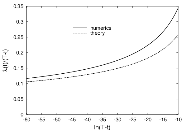
The key question which is left open in this conjecture is: what determines the evolution of the scaling factor ; in particular, what is the asymptotic behaviour of for ? Numerical evidence shown in Figure 7 suggests that the rate of blowup goes asymptotically to zero, that is ()
| (60) |
but it seems very hard to determine an exact asymptotics of from pure numerics44 4 This issue is also discussed by Linhart and Sadun in [14]..
Recently, an analytical approach to this problem has been suggested in [15]. Below we sketch the main idea of this approach. Let be a manifold of rescaled instantons (a one-dimensional center manifold). Assuming that a solution is in a neighbourhood of , we decompose it as
| (61) |
Here represents a small deviation of the solution from and is the collective coordinate on . To fix the splitting between these two parts we require that , where is the projection on . Plugging (61) into (54) we get ()
| (62) |
where is the linear perturbation operator about the instanton
| (63) |
and
| (64) |
It is clear from (62) that , hence for to decay to zero as , the rate of blowup must go to zero as well. We stress this point to emphasize that the linear evolution of , predicted for example by the geodesic approximation, is inconsistent with Conjecture 2. Next, by projecting equation (62) on and in the orthogonal direction, we get a coupled system consisting of a nonhomogeneous wave equation for and an ordinary differential equation for . Solving the first equation for and plugging the result into the second equation, we obtain in the lowest order the following modulation equation
| (65) |
From this we get the leading order asymptotics for
| (66) |
As shown in Figure 7 this result is in rough agreement with numerics. There are many possible sources of the apparent discrepancy. On the numerical side there are discretization errors, an error in estimating the blowup time, or errors in computing from the data. On the analytical side, there might be corrections to (66) coming from the bounded region expansion and, more importantly, from the far field behaviour55 5 The derivation of (65) is not quite straightforward because of the presence of infrared divergencies which need to be regularized.. Finally, and in our opinion most likely reason of discrepancy is that the solution shown in Figure 7 has not yet reached the truly asymptotic regime and consequently the higher order corrections to formula (66) are still significant.
The issue of blowup rate is closely related to the problem of energy concentration in the singularity. To explain this, we define the kinetic and the potential energies at time inside the past light cone of the singularity
| (67) |
Substituting (58) into (67) we obtain
| (68) |
Assuming (60), this implies that
| (69) |
Thus, the energy equal to the energy of the instanton gets concentrated in the singularity. This means that in the process of blowup the excess energy must be radiated away from the inner region as the solution converges to the instanton.
It is worth pointing out that the concentration of energy is a necessary condition for blowup in the critical dimension. To see this, suppose that the solution blows up at time T and assume for contradiction that . Then, by choosing a sufficiently small we can have arbitrarily small. This implies, by causality and global existence for small energy data, that the solution exists globally in time, contradicting the assumption. For radial equations of the type
| (70) |
a stronger result was proved by Struwe [16] who basically showed that if the solution of (70) blows up, then it must do so in the manner described in Conjecture 2. In this sense formation of singularities is intimately tied with the existence of a static solution.
Finally, we address briefly the issue of the threshold of singularity formation. Using the technique described in Section 5, along each interpolating family of initial data we can determine the critical point separating blowup from dispersal. However, in contrast to the case, we see no evidence for the existence of an intermediate attractor in the evolution of nearly critical data. This fact, together with a similar result for dimensional wave maps [6] suggests that in the critical dimension the transition between blowup and dispersal is not governed by any critical solution. We suspect that the evolution of precisely critical initial data still has the form (58) but the dynamics of the scaling factor is different than in (66). This belief is based on the fact that in the evolution of marginally critical initial data we can clearly distinguish a transient phase during which drops very quickly and then, either reaches a minimum and starts growing (in the case of dispersal), or keeps decreasing with the ”normal” rate (in the case of blowup).
8 Conclusions
There are two main lessons that we wanted to convey in this survey. The first lesson is that there are striking analogies between major evolution equations. In particular, the mechanism of blowup to a large extent is determined by the criticality class of the model. These analogies can be used to get insight into hard problems (such as singularity formation for Einstein’s equations) by studying toy models which belong to the same criticality class. This approach is in the spirit of general philosophy expressed by David Hilbert in his famous lecture delivered before the International Congress of Mathematicians at Paris in 1900 [17]: ”In dealing with mathematical problems, specialization plays, as I believe, a still more important part than generalization. Perhaps in most cases where we seek in vain the answer to a question, the cause of the failure lies in the fact that problems simpler and easier than the one in hand have been either not at all or incompletely solved. All depends, then, on finding out these easier problems, and on solving them by means of devices as perfect as possible and of concepts capable of generalization.”
The second lesson is concerned with the interplay between numerical and analytical techniques. Accurate and reliable numerical simulation of singular behaviour is difficult and hard to assess. In order to keep track of a singularity developing on exceedingly small spatio-temporal scales, one needs sophisticated techniques such as adaptive mesh refinement. For these techniques the convergence and error analysis are lacking so extreme care is needed to make sure that the computed singularities are not numerical artifacts. For this reason, in order to feel confident about numerics it is important to have some analytical information, like existence of self-similar solutions. Without a theory, simulations alone do not provide ample evidence for the existence of a singularity. We believe that the interaction between numerical and analytical techniques, illustrated here by the studies of blowup, will become more and more important in future as we begin to attack more difficult problems.
Acknowledgment. I am grateful to Michael Sigal and Yu. N. Ovchinnikov for permission to announce here the results of yet unpublished joint work. I thank Zbislaw Tabor for providing me with data for Figure 7. I acknowledge the hospitality of the Albert Einstein Institute for Gravitational Physics in Golm and the Erwin Schrödinger Institute for Mathematical Physics in Vienna, where parts of this paper were produced.
References
- [1] D. Eardley and V. Moncrief, Commun. Math. Phys. 83, 171 (1982).
- [2] S. Klainerman, in: Progress in Nonlinear Differential Equations and Their Applications, vol.29 (Birkhäuser, 1997).
- [3] T. Cazenave, J. Shatah, and A. Shadi Tahvildar-Zadeh, Ann. Inst. Henri Poincare 68, 315 (1998).
- [4] P. Bizoń, Commun. Math. Phys. 215, 45 (2000).
- [5] P. Bizoń, T. Chmaj, and Z. Tabor, Nonlinearity 13, 1411 (2000).
- [6] P. Bizoń, T. Chmaj, and Z. Tabor, Nonlinearity 14, 1041 (2001).
- [7] P. Bizoń and Z. Tabor, Phys. Rev. D64, 121701 (2001).
- [8] O. Dumitrascu, Stud. Cerc. Mat. 34(4), 329 (1982).
- [9] S. Klainerman and M. Machedon, Ann. Math. 142, 39 (1995).
- [10] P. Breitenlohner, P. Forgács, and D. Maison, Commun. Math. Phys. 163, 141 (1994).
- [11] M. W. Choptuik, Phys. Rev. Lett. 70 , 9 (1993).
- [12] C. Gundlach, Living Rev. Relativity 2(4) (1999).
- [13] S. L. Liebling, E. Hirschmann, and J. Isenberg, J.Math.Phys. 41, 5691 (2000).
- [14] J. M. Linhart and L. A. Sadun, Nonlinearity 15, 219 (2002).
- [15] P. Bizoń, Yu. N. Ovchinnikov, and I. M. Sigal, in preparation.
- [16] M. Struwe, preprint (2000), to appear in Comm. Pure Appl. Math.
- [17] D. Hilbert, reprinted in: Bull. Amer. Math. Soc. 37, 407 (2000).