Gerbes, covariant derivatives, -form lattice gauge theory, and the Yang-Baxter equation
Abstract
In -form lattice gauge theory, the fluctuating variables live on -dimensional cells and interact around -dimensional cells. It has been argued that the continuum version of this model should be described by -gerbes. However, only connections and curvatures for gerbes are understood, not covariant derivatives. Using the lattice analogy, an alternative definition of gerbes is proposed: sections are functions , were is the base point and is the surface element. In this purely local formalism, there is a natural covariant derivative. The Yang-Baxter equation, and more generally the simplex equations, arise as zero-curvature conditions. The action of algebras of vector fields and gerbe gauge transformations, and their abelian extensions, are described.
1 Introduction
Gerbes have recently attracted considerable attention. Apart from being of intrinsic mathematical interest [9, 10, 15], they appear in Hamiltonian quantization [12] and in brane models [11, 29]. There also seem to be close ties between gerbes and n-category theory [5, 13]
My interest in this subject arose when I tried to understand lattice integrable statistical models. As is well known, the quantum Yang-Baxter equation (QYBE) is a sufficient (and in practise necessary) condition integrability in two dimensions [6]. The analogous sufficient condition in three dimensions is Zamolodchikov’s tetrahedron equation [4, 8, 7, 28], and in dimensions it is the so-called -simplex equation. Unfortunately, very few solutions to the tetrahedron equation are known, and those that are known do not depend on any temperature-like parameters.
Long ago I observed a striking similarity between the QYBE and the zero-curvature condition in lattice gauge theory. This lead me to formulate a statistical model where the fluctuating variables live on plaquettes rather than links [18]. In section 2 this model is reviewed, and a serious flaw is corrected: it is necessary to assign several variables to each plaquette. An important feature of this model is that the gauge-invariant holonomy is given by two-dimensional “Wilson surfaces”. The generalization to higher-dimensional models is now obvious: the variables live on -cells and there is holonomy associated to -dimensional “Wilson submanifolds”.
The continuum limit of this kind of model is -form electromagnetism in the abelian case, and in general it is a gauge theory on loop space. The first such model was probably written down by Freund and Nepomechie [14], but already a few years before had Polyakov noted that ordinary gauge theory can be formulated as a sigma model in loop space [25, 26]. This immediately suggests that continuum integrability in higher dimensions is best understood in terms of flat connections on gerbes, which is closely related to BF theory [1].
Whereas a theory of connections on abelian gerbes has been around for a few years [15, 19], the situation for non-abelian gerbes is very tentative. Various suggestions, whose mutual relations are unclear to me, can be found in [2, 3, 9, 20]. What does not seem right, neither from the loop space approach or from lattice gauge theory, is the appearence of a hierarchy of connections. Another problem with the gerbe and BF approaches is that there seems to be no natural covariant derivative. This is a serious drawback since the main interest in connections is their relation to parallel transport. The standard approach to gerbes is reviewed in Section 3.
To remedy these problems, I suggest an alternative definition of gerbes in Section 4. The main idea is that a gerbe section is a function not only of the spacetime point , but also a function of the direction . A gerbe section is a functional on loops over , the local information about which is encoded in the point and the direction of the loop passing through . The generalization to higher gerbes is obvious, and in fact we mainly formulate the results for -gerbes. In this way, a manifestly local tensor calculus is developed, which should be useful for explicit calculations. We construct covariant derivatives, connections and curvatures and check that all constructions are invariant both under infinitesimal spacetime diffeomorphisms and under gerbe gauge transformations.
Flatness of the gerbe connection gives rise to the classical Yang-Baxter equation in a particular gauge, which again indicates relevance for higher-dimensional integrability. Finally, it is shown how -form electromagnetism can be recovered in the abelian case. The language developed in the present paper is thus appropriate for the non-abelian generalization of -form electromagnetism, which is known to be impossible using ordinary bundles [27].
2 A generalization of lattice gauge theory
Recall that in ordinary lattice gauge theory [16], the amplitude for parallel transport along a link from to is the matrix
| (2.1) |
where is the lattice spacing and is the :th component of the gauge potential. Here is a point on an -dimensional hypercubic lattice and denotes a unit vector in the :th direction. If a particle is transported along a link and then back again, nothing has happened, so we associate the matrix with the same link with the opposite orientation. The curvature is given by the holonomy around a plaquette, which is the smallest loop that can be constructed.
| (2.2) |
The action reads
| (2.3) |
We see that in the limit that the lattice spacing , this becomes the Yang-Mills action, at least formally. There is a gauge symmetry associated to each vertex; the transformation
| (2.4) |
leaves the action (2.3) invariant. The gauge invariant observables are Wilson loops, i.e. the product of matrices around a closed loop.
Instead of putting matrices on links, it is natural to put four-index quantites on plaquettes. Associate a vector space to each link, and an element to a plaquette in the -plane. is in fact an element acting on , where is the number of dimensions, but it acts as the identity except on the :th and :th factors. We can interpret as the amplitude for parallel transport of a string element across the plaquette.

In fact, and this is something which I missed in [18], two independent variables are needed for each plaquette. can be interpreted as the amplitude for parallel transport of a string element across the NE diagonal, as illustrated in Figure 1. It is then clear that four such amplitudes are needed, one each for the four different directed diagonals. However, only two amplitudes are independent, since and .

To every triangulated surface , we can associate a holonomy by contracting indices associated to links were two plaquettes are glued together. This holonomy is the amplitude for transport of a string across the surface. As we see in Figure 2, there is a natural notion of associativity. Since we now have a vector space associated to each link on the boundary of the Wilson surface,
| (2.5) |
The curvature is the infinitesimal holonomy associated to each elementary cube. E.g., for a cube in the -direction one has
| (2.6) | |||
and the action reads
| (2.7) |
The eight terms corresponds to the cube’s eight directed diagonals. Just as the two terms in ordinary lattice gauge theory can be interpreted as parallel transport of a particle around the plaquette, in the clockwise and counter-clockwise directions, the eight terms here rotate a string piece around the cube’s diagonals.
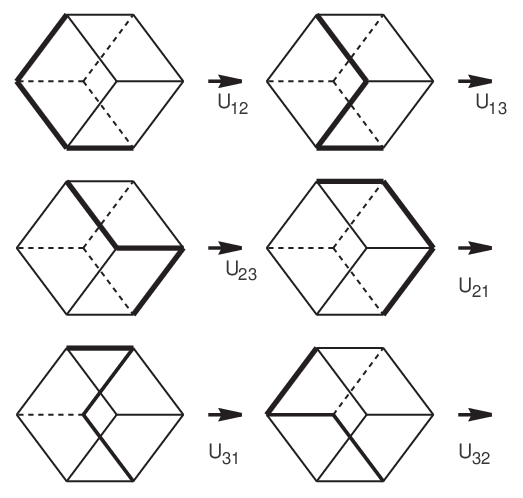
There is a gauge symmetry associated to each link; the transformation
| (2.8) |
leaves the action invariant. The gauge invariant observables are closed Wilson surfaces, i.e. the product of four-index objects around a closed, two-dimensional surface. The natural continuum formulations of this model are in terms of loop or membrane variables (non-zero and zero curvature, respectively). Locality is not manifest in these formulations, but it is clear on the lattice that the model is perfectly local; the action is a sum over elementary cubes.

The zero-curvature condition is quite interesting. In the spatially homogeneous case (objects depend on orientation but not on location), zero 1-curvature becomes , i.e. and commute. Vanishing -curvature becomes
| (2.9) |
which is the Yang-Baxter equation, of paramount importance to the theory of integrable lattice models in two dimensions. The standard illustration of the Yang-Baxter equation is the equality of two cube halves, as shown in Figure 4.
It is immediate how to generalize this model to -Yang Mills theory on the lattice. The zero -curvature condition is known as the -simplex equation. It is sufficient to construct integrable lattice models in dimensions, but unfortunately no interesting solutions to it are known. More precisely, some solutions are known, but one needs a continuum of solutions depending on variables like temperature or magnetic field to be able to compute critical exponents.
3 Gerbes
3.1 Bundles
Let us first review the definition of an ordinary line bundle over an -dimensional manifold . Start with a good cover of . Each neighborhood looks like , and on the overlaps we define transition functions with values in . We can illustrate each neighborhood by a and the overlap, or rather the transition function, as an arrow between bullets:
The transition functions must satisfy the consistency conditions
which can be illustrated by the following diagrams
i.e. going round a triangle results in the unit operator. These conditions make into a Cech cocycle in .
Two manifolds and are equivalent if there exist functions on such that
| (3.11) |
corresponding to the picture
This is already very reminiscent of a lattice gauge theory with neighborhoods playing the role of points and transition functions the role of amplitudes, and the equivalence relation is recognized as a gauge transformation.
3.2 Gerbes
A gerbe (more precisely, 1-gerbe) is a generalizion of a bundle. On every triple overlap we define a function , which can be illustrated by the oriented triangle
The transition functions satisfy
| (3.12) |
and the cocycle condition on quadruple overlaps
| (3.13) |
This condition corresponds to a tetrahedron diagram. Two gerbes and are equivalent if there are functions living on double overlaps (i.e. the edges of the triangle), such that
| (3.14) |
These conditions make into a Cech cocycle in . Again there is striking resemblance with the lattice 2-gauge theory I described: the transition function lives on a plaquette, there is a gauge invariance living on the link, and a curvature associated to a -dimensional cell. The main difference is that two-form lattice gauge theory involves square plaquettes whereas the gerbe picture gives rise to triangles.
It is now straightforward to extend the definitions to -gerbes in terms of functions living on -fold overlaps and satisfying cocycle conditions on -fold overlaps. In particular, bundles = 0-gerbes and gerbes = 1-gerbes.
3.3 Connections on abelian bundles
Define a one-form on and a global two-form by
Two bundles and with connections and are equivalent if with equivalence (3.14) and
| (3.18) |
3.4 Connections on abelian gerbes
Define a one-form on , a two-form on and a global three-form .
Two gerbes and with gerbe-connections , and , are equivalent if and
Note the trade-off between overlap and spacetime indices (form degree).
3.5 Connection on non-abelian gerbes
The treatment of abelian gerbes seems rather well established. However, if one wants to identify the Yang-Baxter equation with a flatness condition for gerbe connection, one must consider non-abelian gerbes; the Yang-Baxter equation is not very interesting if is abelian.
Mackaay [20] defines local one-forms , valued in the Lie algebra of , such that
| (3.25) |
Two gerbes , and , with connections , , and , , are equivalent if there exists such that
| (3.26) |
3.6 Local expressions for gerbe connections and curvatures
Locally, a bundle connection is a -valued one-form and the curvature is a -valued two-form , where . The Bianchi identity reads .
Attal [3] introduces the following data11 1 Attal uses different letters. to describe a gerbe connection: a -valued one-form (connection) and an -valued two-form (curving), whose curvatures are given by a -valued two-form and a -valued three-form , where
| (3.27) | |||||
The Bianchi identity
| (3.28) |
follows from and the Jacobi identity.
However, this formulation seems unsuitable to describe the generalized lattice model in Section 2, for several reasons.
- •
A hierarchy of connections arises in the continuum description but only the top -form connection appears on the lattice.
- •
The modified curvature is the usual curvature of the one-form connection .
- •
There is no natural covariant derivative.
- •
There seems to be no natural place for the Yang-Baxter equation.
With these problems in mind, I propose an alternative local formulation of gerbes in the next section.
4 Gerbes in local coordinates
4.1 Symmetries
Locally, the gerbe coordinates are , where , is a point in the underlying space , and , is a -dimensional surface element. We have . For definiteness, we will mainly consider the case in the sequel, but all formulas are readily generalized to arbitrary , and later the case will receive special attention. Introduce derivatives and , satisfying the Heisenberg algebra
| (4.29) |
Let be a vector field acting on the base space . The algebra of vector fields , i.e. the algebra of infinitesimal diffeomorphisms, can be realized as
where both
| (4.31) |
and satisfy :
| (4.32) |
Let be the generators of a finite-dimensional Lie algebra with structure constants , i.e.
| (4.33) |
Then generates an algebra of gerbe gauge transformations, which we call the gerbe gauge algebra and denote by . Note that depends on both the base point and the surface element , but only depends on . The brackets in read
| (4.34) | |||||
Observe the second term in the middle equation, which is absent for ordinary gauge transformations. The Lie derivatives () and satisfy the same algebra:
| (4.35) | |||||
provided that .
4.2 Sections and connections
A gerbe section corresponds locally to a tensor field valued in a module. If the action is given by and the action by , then carries the following representation of :
Here and henceforth we suppress arguments, and keep in mind that all fields and functions (, , etc) depend on , except vector fields which only depend on . It follows immediately from () that the derivative transforms as
Now define the covariant derivative
| (4.38) |
which is covariant only w.r.t. , and
| (4.39) |
which is covariant w.r.t. all of . The connections and (which both depend on both and ) transform as
| (4.41) | |||||
The consistency of these transformation laws follow immediately because both the covariant derivative and the ordinary derivative transform consistently, and hence so does their difference.
For brevity, we sometimes write , , and . The associated curvature is
| (4.42) |
where
| (4.43) | |||||
Note that the derivative of need covariantization because it is a (-valued) function of both and :
| (4.44) |
Apart from the ordinary derivative w.r.t. , we must also convariantize the gerbe derivative . From
| (4.45) | |||||
we see that transforms under as a tensor with two extra indices, but the action needs compensation. Introduce
| (4.46) |
It follows that
| (4.47) |
The associated curvature is
| (4.48) |
One can also define the “cross curvature” .
4.3 Rescaling invariance
We can use the covariant gerbe derivative to impose invariance under surface rescalings. One immediately checks that and transform in the same way under . Therefore we can consistently impose the constraint
| (4.49) |
for any constant .
Alternatively, we may consider invariance under rescalings of the surface elements as a symmetry. Consider gerbe sections which are invariant under transformations of the form . Moreover, we let rescalings depend on the base point , so infinitesimally for some function . The rescaling satisfies
| (4.50) | |||||
in addition to the brackets in (4.34). Eq. (4.35) is supplemented by
| (4.51) | |||||
In the parlance of constrained systems, generates a gauge symmetry. The constraint is first class, which together with the gauge condition (4.49) becomes a second class constraint.
Introduce two generators and , satisfying the algebra
| (4.52) | |||||
Then it turns out that the rescalings can be realized as
| (4.53) |
To prove that (4.53) indeed furnishes a realization of the rescaling algebra, it is useful to introduce the abbreviations
| (4.54) |
It is clear that
and that we can rewrite (4.53) as
| (4.56) |
4.4 A special gauge choice
Assume that we require
| (4.57) |
where . In coordinate-free notation is a -valued three-form. This choice is obviously not preserved by , but we may hope that it preserved by the subalgebra generated by ’s of the form
| (4.58) |
The transformation law () becomes
| (4.59) |
where
| (4.60) |
A sufficient condition for this to hold is clearly
| (4.61) |
In coordinate-free notation, this reads , where is the contraction of the two-form and the two-vector . The associated curvature can now be written
| (4.62) |
where is totally anti-symmetric in spacetime indices and
| (4.63) |
In coordinate-free notation, the four-form transforms as under .
However, the consistency of (4.57) requires not only (4.61), but it also relies on the assumption that the gauge choice (4.58) defines a subalgebra. One checks that the commutator of two fields of the form (4.58),
| (4.64) |
is in general not of the same form unless . Hence the choice (4.57) is not invariant even under the subalgebra (4.58) of if is non-abelian.
4.5 Gerbe holonomy
Let be a closed three-dimensional manifold with local coordinates , where . We have thus choosen a foliation of . Now regard as a submanifold , with the embedding given by coordinate functions . The surface element becomes on
| (4.65) |
If is abelian, we define the holonomy
| (4.66) |
One checks that is invariant under the gerbe gauge algebra:
since the integral vanishes. Diffeomorphism invariance is also clear.
If we make the special gauge choice (4.57), the holonomy becomes
| (4.68) | |||||
since
| (4.69) |
for some constant . The holonomy (4.68) is invariant under the restricted set of gauge transformations (4.58), because
| (4.70) |
and the boundary by assumption.
Let us now turn to the case non-abelian. In the ordinary one-form gauge theory case, the exponential of the integral must be replaced by the path-ordered integral:
| (4.71) |
where is some curve. This formal expression is most intuitively defined in the lattice approximation. In particular, satisfies the relation , where is the concatenation of and .
Analogously, we now define the surface-ordered integral
| (4.72) |
by its lattice regularization. In particular, takes values in the space , which should be thought of as the continuum analogue of (2.5). The size of the space (a continuum tensor product) makes the expression (4.72) merely formal, in contrast to the manifestly well-defined local expressions like (4.38) and (4.43).
4.6 Gerbe Yang-Mills theory
In this subsection we assume that there is a preserved constant (and thus flat) metric with inverse , and hence that diffeomorphism invariance is broken down to Poincaré invariance. This means that , so we can ignore the difference between the covariant derivatives and (4.38), (4.39).
The natural gerbe generalization of the pure Yang-Mills action is
| (4.73) |
which leads to the Yang-Mills equations
| (4.74) |
In particular, if we assume that the connection is of the form (4.57), we recover the equations of motion of -form electromagnetism in the abelian case:
| (4.75) |
The gerbe equations (4.74) are thus the natural non-abelian generalization of -form electromagnetism.
4.7 The classical Yang-Baxter equation
In the previous subsections all formulas were specialized to the case , but the analogous formulas for arbitrary are readily deduced. We here set , so the line coordinate becomes a one-vector. If we make the gauge choice analogous to (4.57), so the connection is given by a two-form , the curvature three-form becomes
| (4.76) |
This gauge choice is of course completely non-invariant.
Let be spatially homogeneous, i.e. it does not depend on at all, so the first term above vanishes. Moreover, consider the special point in three dimensions. The zero-curvature condition then exlicitly becomes
This is recognized as the classical Yang-Baxter equation (CYBE). That this equation arises in the continuum formulation is hardly surprising since we have seen that the QYBE appears on the lattice.
As is well known, the CYBE is an equation on the triple space , where is a vector space associated to a link, and acts non-trivially on only: , etc. The simplest class of solutions are the trigonometric ones of the form
| (4.78) |
where are the generators of and we have contracted indices using the Killing metric on . Note that the solution depends on additional, “spectral” parameters. If we collect these into a vector we may write
| (4.79) |
etc.
Returning to , vanishing of the curvature four-form (4.63), , becomes in the spatially homogeneous case and at the point :
This is the infinitesimal form of Zamolodchikov’s tetrahedron equation [4, 8, 7, 28]. It is an equation in the space , such that acts trivially on all spaces except .
The classical tetrahedron equation () has a rather disquiting property. Of the six terms, the only one that is non-trivial on all factors except is . Therefore, this expression can in fact not act non-trivially on all of , but it rather consists of terms that act on four spaces only. The natural ansatz is , where is a solution of the Yang-Baxter equation. I am not aware of any genuine solutions to ().
The generalization to higher order is obvious.
4.8 Abelian extensions
Upon quantization, we expect the gerbe gauge algebra to acquire an abelian extension. To construct representations of such extensions following [17], we introduce a one-dimensional closed curve , , where , and expand all fields in a Taylor around :
| (4.81) |
where and , all , () are multi-indices of length and , respectively. Moreover,
| (4.82) |
and similar for .
After introducing canonical momenta for , and and normal ordering, we obtain Fock representations of the following algebra:
| (4.83) | |||||
where is the Killing metric in and
Equation (4.83) is the gerbe analogue of the Virasoro and affine Kac-Moody algebras, and the abelian charges , and can be computed with the methods of [17].
5 Conclusion
In this paper I have developed a local continuum formulation of the -form lattice gauge theory in Section 2. Holonomy is an integral over -dimensional Wilson submanifolds, as in (2.5) and (4.72), making this theory closely related to -gerbes. However, there are some advantages compared to other formulations:
- •
A natural covariant derivative exists.
- •
There is only a -form connection, not a hierarchy of connections.
- •
The relation to integrability, i.e. the quantum and classical Yang-Baxter equations, is clear.
The main advantage compared to formulations in loop space is manifest locality, which should facilitate explicit calculations.
References
- [1] O. Alvarez, L. A. Ferreira and J. Sànchez Guillén, A new approach to integrable theories in any dimension, hep-th/9710147 (1997).
- [2] R. Attal, Two-dimensional parallel transport: combinatorics and functoriality, math-ph/010505 (2001).
- [3] R. Attal, Combinatorics of non-abelian gerbes with connection and curvature, math-ph/0203056 (2002).
- [4] V. V. Bazhanov and Yu. G. Stroganov, Nucl. Phys. B230 [FS10] (1984) 435.
- [5] J. C. Baez and J. Dolan, Higher-dimensional algebra and topological quantum field theory, J. Math. Phys 36 (1995) 11.
- [6] R. J. Baxter, Exactly solved models in statistical mechanics, Academic Press, London (1982).
- [7] R. J. Baxter and P. J. Forrester, Is the Zamolodchikov model critical?, J. Phys. A 18 (1986) 1483–1497.
- [8] R. J. Baxter, On Zamolodchikov’s solution of the tetrahedron equations, Comm. Math. Phys. 88 (1983) 185–205.
- [9] L. Breen and W. Messing, Differential geometry of gerbes, math.AG/0106083 (2001).
- [10] J.-L. Brylinski, Loop spaces, characteristic classes and geometric quantization, Prog. in Math. vol. 107, Birkhäuser, Boston (1993).
- [11] M. I. Caicedo, I. Martin and A. Restuccia, Gerbes and duality, hep-th/0205002 (2002).
- [12] A. L. Carey, J. Mickelsson and M. K. Murray, Bundle gerbes applied to quantum field theory, hep-th/9711133 (1997).
- [13] D. Freed, Higher algebraic structures and quantization, Comm. Math. Phys. 159 (1994) 343–398.
- [14] P. G. O. Freund and R. Nepomechie, Nucl. Phys. B199 (1982) 482.
- [15] N. Hitchin, Lectures on special Lagrangian submanifolds, math.DG/9907034 (1999).
- [16] J. Kogut, An introduction to lattice gauge theory and spin systems, Rev. Mod. Phys. 51 (1979) 659–713.
- [17] T. A. Larsson, Extended diffeomorphism algebras and trajectories in jet space. Commun. Math. Phys. 214 (2000) 469–491.
- [18] T. A. Larsson, -cell gauge theories, manifold space and multi-dimensional integrability, Mod Phys Lett A 5 (1990) 255–264.
- [19] M. Mackaay and R. Picken, Holonomy and parallel transport for abelian gerbes, math.DG/0007053 (2001).
- [20] M. Mackaay, A note on the holonomy of connetions in twisted bundles, math.DG/0106019 (2001).
- [21] R. Nepomechie, Nuclear Physics B212 (1983) 310.
- [22] P. Orland, Physics Letters 122B (1983) 78.
- [23] P. Orland in Gauge Theory on Lattice: 1984, Proceedings of the Argonne Ntional Laboratory Workshop, National Technical Information Service, Springfield, VA, USA (1984), page 305.
- [24] P. Orland, Imperial College preprint, July 1984. http://ccdb3fs.kek.jp/cgi-bin/img_index?8408054
- [25] A. M. Polyakov, Phys. Lett. 82B (1979) 247; Nucl. Phys. B164 (1979) 171.
- [26] A. M. Polyakov, Gauge fields and strings, Harwood, Chur (1987).
- [27] C. Teitelboim, Phys. Lett. 167B (1986) 63.
- [28] A. B. Zamolodchikov, Tetrahedron equations and the relativistic S-matrix of straight-strings in 2+1-dimensions, Comm. Math. Phys. 79 (1981) 489 – 505.
- [29] Y. Zunger, p-Gerbes and Extended Objects in String Theory, hep-th/0002074 (2000)