Instantaneous frequency and amplitude identification using wavelets: Application to glass structure

J.D. Harrop, S.N. Taraskin, and S.R. Elliott Affiliation: Department of Chemistry, University of Cambridge, Cambridge CB2 1EW, UK.

15 February 2002

Abstract

This paper describes a method for extracting rapidly varying, superimposed amplitude- and frequency-modulated signal components. The method is based upon the continuous wavelet transform (CWT) and uses a new wavelet which is a modification to the well-known Morlet wavelet to allow analysis at high resolution. In order to interpret the CWT of a signal correctly, an approximate analytic expression for the CWT of an oscillatory signal is examined via a stationary-phase approximation. This analysis is specialized for the new wavelet and the results are used to construct expressions for the amplitude and frequency modulations of the components in a signal from the transform of the signal. The method is tested on a representative, variable-frequency signal as an example before being applied to a function of interest in our subject area - a structural correlation function of a disordered material - which immediately reveals previously undetected features.

pacs

61.43.Bn, 61.43.Fg, 02.30.Nw, 02.70.Hm

I Introduction

Although the first example of a wavelet basis dates back to 1910 Haar 1910, it was not until the early 1980’s, with the work of Goupillaud, Morlet and Grossmann Goupillaud et al. 1984 in seismic geophysics, that the wavelet transform (WT) became a popular tool for the analysis of signals with non-periodic characteristics, termed non-stationary signals van den Berg 1999.

The WT allows a signal to be examined in both the time- and frequency-domains simultaneously. The WT as a time-frequency method has replaced the conventional Fourier transform (FT) in many practical applications. The WT has been successfully applied in many areas of physics van den Berg 1999 including astrophysics, seismic geophysics, turbulence and quantum mechanics, as well as many other fields including image processing, biological signal analysis, genomic DNA analysis, speech recognition, computer graphics and multifractal analysis.

The term WT is conventionally used to refer to a broad selection of transformation methods and algorithms. In all cases, the essence of a WT is to expand the input function in terms of oscillations which are localized in both time and frequency.

Different applications of the WT have different requirements. Image compression, for example, often uses the discrete WT (DWT) to transform data to a new, orthogonal basis set where the data are hopefully presented in a more redundant form Prasad and Iyengar 1997. Other applications, particularly signal analysis Silverman and Vassilicos 2000, use the CWT, sacrificing orthogonality for extra precision in the identification of features in a signal.

The principal aim of this paper is to present the WT in a form well suited to the analysis of one-dimensional signals whose frequency components have rapidly varying frequency and amplitude modulations. In order to achieve this aim, we introduce a new ‘tunable’, complex wavelet. This wavelet is based upon the well-known Morlet wavelet Goupillaud et al. 1984 but is better suited to high-resolution analysis. The features of the WT using the proposed wavelet are understood through an asymptotic stationary-phase approximation to the integral expression of the WT specialized to the new wavelet. We demonstrate the properties of the WT using two example functions, a mathematical function and the other a realistic physical model function.

We are interested in exploiting the complex WT in the analysis of structural correlation functions which describe the atomic structure of disordered materials. As these correlation functions have different spatial regimes, they may be classed as non-stationary signals. Despite the overwhelming success of the WT in other fields, we are aware of only one other paper on this application of the WT. In that application, Ding et al. Ding et al. 1998 studied an experimentally observed correlation function of vitreous silica using the Mexican Hat wavelet. We improve upon this single, prior application in three significant ways, namely the use of the complex WT, a ‘tunable’ wavelet and the method of interpreting the resulting transforms.

We then analyze the reduced radial distribution function (RRDF) of a structural model of a one-component glass with pronounced icosahedral local order Dzugutov 1993. The resulting WT clearly shows the existence of different frequency components in the RRDF and their exponential decay. These features were not clearly detectable by earlier methods (c.f. Ref. Ding et al. 1998).

In Sec. II we review the mathematical framework of the wavelet transform and discuss some mother wavelet functions before modifying an existing wavelet for our purposes. In Sec. III.1 we consider the WT of a general oscillatory signal using the new wavelet. The results are then used to interpret the wavelet transforms of a variable-frequency example function in Sec. III.2 and of the RRDF in Sec. III.3. Concluding remarks can be found in Sec. IV.

II Formulation

The underlying WT used in this paper can be completely described as a one-dimensional complex, continuous WT using wavelets of constant shape Daubechies 1992. We begin by examining the formulation of this WT in terms of an integral transform, before examining the choice of mother wavelet function.

For simplicity we use time-frequency terminology, considering the signal to be an input function of time, $f(t)$ . The CWT is an integral transformation which expands an input function $f(t)$ in terms of a complete set of basis functions $\xi(t;a,b)$ . These basis functions are all the same shape as they are defined in terms of dilation by $a$ and translation by $b$ of a mother wavelet function $\psi(t)$ :

\xi(t;a,b)=|a|^{-1}\psi\!\left(\frac{t-b}{a}\right),

(1)

with $a,b\in\mathbb{R}$ and $a\neq 0$ .

The CWT $F(a,b)$ is defined as the inner product:

F(a,b)=\left\langle\xi|f\right\rangle\equiv|a|^{-1}\int_{-\infty}^{\infty}\psi^{*}\!\left(\frac{t-b}{a}\right)\,f(t)\,dt.

(2)

The original formulation of the CWT Goupillaud et al. 1984 used a prefactor $|a|^{-\frac{1}{2}}$ to give a normalization to unity, $\left\langle\xi|\xi\right\rangle=1$ ). We choose an alternative prefactor $|a|^{-1}$ (giving $\left\langle\xi|\xi\right\rangle=|a|^{-1}$ ) after Delprat et al. Delprat et al. 1991. As we shall see, this formulation of the CWT allows for simple frequency identification by examining the maxima in the modulus of the CWT with respect to the scale $a$ .

In order to understand the CWT, it is useful to relate it to the FT. The FT has a non-localized, plane-wave basis set and, therefore, has a single transform parameter - the frequency $\omega$ . In contrast, the basis set of the CWT contains localized oscillations characterised by two transform parameters - the scale (or dilation) $a$ and the translation (or position) $b$ . It is this critical difference which makes the CWT preferable for the analysis of non-stationary signals.

We are free to choose a functional form for $\psi(t)$ , subject to some constraints. Some of these constraints are forced upon us whereas others arise from the practical usefulness of the resulting transform.

In order to recover a function from its wavelet transform via the resolution of the identity Daubechies 1992, $\psi(t)$ must satisfy an admissibility condition. Although we do not make direct use of the resolution of the identity in this paper, we require that our choice of $\psi(t)$ satisfies this condition to ensure that all information about the signal is retained by the transform. The admissibility condition is essentially that the FT, $\hat{\psi}(\omega)=\left\langle e^{i\omega t}|\psi\right\rangle$ , satisfies the relation $\hat{\psi}(0)=0$ , equivalent to requiring that the mother wavelet and, hence, the basis wavelets, have a mean of zero.

Beyond simply satisfying the admissibility condition, it is practically useful to create mother wavelet functions which mimic features of interest in the signal. In the case of time-frequency analysis, mother wavelet functions are chosen which represent localized sinusoidal oscillations. The resulting wavelet transforms can then be used to extract instantaneous measures of frequency and amplitude. The uncertainty principle dictates that the product $\Delta t\Delta\omega$ of the time and frequency uncertainties of such wavelets has a lower bound. It is no surprise, therefore, that this class of mother wavelet functions are typically based upon Gaussians. However, it is still possible to trade temporal precision for frequency precision by altering the number of oscillations in the envelope of the mother wavelet.

The simplest such wavelet is the “Mexican Hat” wavelet which mimics a single oscillation and is commonly used in signal analysis. The functional form of this wavelet is the second derivative of a Gaussian. This wavelet offers good localisation in the time domain whilst retaining admissibility. However, this wavelet has two major drawbacks for general signal analysis: (i) useful information can only be extracted from the WT at discrete intervals where the wavelets are in phase with the signal, and (ii) the time-frequency resolution is fixed.

The former drawback has been overcome by the invention of complex wavelets which mimic localized plane waves. The WT can be computed separately for the real and imaginary parts, yielding a complex scalar field, $F(a,b)$ , where the modulus and argument of $F$ represent the amplitude and phase of the signal, respectively.

The latter drawback has been overcome by the invention of tunable wavelets which include an additional parameter to the mother wavelet function controlling the number of oscillations in the envelope.

Goupillaud, Morlet and Grossman overcame these problems simultaneously with the invention of a modulated Gaussian wavelet, now known as the “Morlet” wavelet Goupillaud et al. 1984. This wavelet has a parameter, $\sigma$ , which controls the number of oscillations in the envelope, allowing time and frequency uncertainties to be traded. Thus the Morlet wavelet can be expressed as:

\displaystyle\psi_{\textrm{M}}(t;\sigma)

\displaystyle=

\displaystyle\pi^{-\frac{1}{4}}c_{\textrm{M}}(\sigma)\,e^{-\frac{1}{2}t^{2}}\left(e^{i\sigma t}-\kappa(\sigma)\right),

(3)

where $c_{\textrm{M}}(\sigma)=(1-2e^{-\frac{1}{4}\sigma^{2}}\kappa(\sigma)+\kappa^{2}(\sigma))^{-1/2}$ and the parameter $\kappa(\sigma)$ allows the admissibility condition to be satisfied.

The FT of this wavelet is:

\displaystyle\hat{\psi}_{\textrm{M}}(\omega;\sigma)

\displaystyle=

\displaystyle\pi^{-\frac{1}{4}}c_{\textrm{M}}(\sigma)\left(e^{-\frac{1}{2}\left(\omega-\sigma\right)^{2}}-\kappa(\sigma)\,e^{-\frac{1}{2}\omega^{2}}\right).

(4)

From Eq. (4) it is clear that the admissibility condition $\hat{\psi}_{\textrm{M}}(0;\sigma)=0$ implies that $\kappa(\sigma)=e^{-\frac{1}{2}\sigma^{2}}.$

Many previous applications of the Morlet wavelet have been concerned with signals containing slowly varying frequency and amplitude components for which large values of $\sigma$ ( $\geq 5$ ) are applicable and $\kappa(\sigma)$ ( $\leq 10^{-6}$ ) is negligible Goupillaud et al. 1984.

However, we are interested in applying this type of analysis to signals which contain rapidly varying frequencies and amplitudes. In this case, the ability to use small values of $\sigma$ becomes important as we wish to maximize the temporal resolution by minimizing $\sigma$ whilst still being able to separate the various frequency components in the signal and, consequently, $\kappa(\sigma)$ is no longer negligible.

Although the Morlet wavelet is admissible at small $\sigma$ , the temporal localization is unsatisfactory (see Fig. 1); namely, $|\psi_{\textrm{M}}|^{2}$ undergoes a transition from mono-modality to bimodality (a single ridge at large $\sigma$ splits into two symmetric ridges for small $\sigma$ ). The wavelet transform of a signal performed using a wavelet which has a bimodal envelope results in the signal being localized about two different positions (see Fig. 2). This produces unwanted artefacts in the resulting instantaneous frequency and amplitude measurements (shown later in Figs. 10 and 11).

Refer to caption — Figure 1: Envelope $|\psi_{\textrm{M}}|^{2}$ of the Morlet wavelet $\psi_{\textrm{M}}(t;\sigma)$ (Eq. 3) showing the unwanted transition from mono-modal to bimodal behaviour at small $\sigma$ ( $<1.79785$ ).

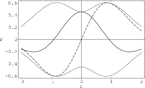
Therefore we remedy this drawback by modifying the Morlet wavelet to produce a new wavelet, $\psi(t;\sigma)$ , such that $|\psi|^{2}$ has a single, global maximum for all $\sigma$ . For the new wavelet we choose to replace the single, normalization constant $c_{\textrm{M}}(\sigma)$ in the Morlet wavelet with two new parameters $p(\sigma)$ and $q(\sigma)$ determined by two conditions: (i) total normalization of the wavelet to unity, and (ii) equal contributions to the normalization from the real and imaginary parts. The new wavelet has the following functional form:

	$\displaystyle\psi(t;\sigma)$	$\displaystyle=\,\pi^{-\frac{1}{4}}e^{-\frac{1}{2}t^{2}}\!\!\!$	$\displaystyle\left[p(\sigma)\left(\cos(\sigma t)-\kappa(\sigma)\right)\right.$		(5)
			$\displaystyle\left.+\,i\,q(\sigma)\sin(\sigma t)\right],$		(5)

where $p(\sigma)$ and $q(\sigma)$ are given by:


$\displaystyle p(\sigma)$	$\displaystyle=$	$\displaystyle\left(1-e^{-\sigma^{2}}\right)^{-\frac{1}{2}},$	(6a)
$\displaystyle q(\sigma)$	$\displaystyle=$	$\displaystyle\left(1+3e^{-\sigma^{2}}-4e^{-\frac{3}{4}\sigma^{2}}\right)^{-\frac{1}{2}}.$	(6b)

The Fourier transform of this wavelet is:

	$\displaystyle\hat{\psi}(\omega;\sigma)$	$\displaystyle=$	$\displaystyle\frac{1}{2}e^{-\frac{1}{2}\left(\sigma+\omega\right)^{2}}\left(e^{\sigma\omega}-1\right)$		(7)
			$\displaystyle\times\left[\left(e^{\sigma\omega}-1\right)p(\sigma)+\left(e^{\sigma\omega}+1\right)q(\sigma)\right].$		(7)

It is worthwhile noting that the real part of this new wavelet recovers the functional form of the Mexican Hat wavelet in the limit $\sigma\rightarrow 0$ :

\textrm{Re}\left[\psi(t;0)\right]=\sqrt{\frac{2}{3}}\pi^{-\frac{1}{4}}e^{-\frac{1}{2}t^{2}}(t^{2}-1).

Thus the new wavelet allows a complete transition from very high temporal localization, $\sigma\rightarrow 0$ (the Mexican Hat wavelet), to maximum frequency localization, $\sigma\rightarrow\infty$ (plane wave). Even in the limit of minimal $\sigma$ , $|\psi|^{2}$ remains mono-modal (see Figs. 3 and 4). Thus we have improved upon the temporal localisation of the Morlet wavelet.

We have also checked that, using the new wavelet, the original signal can be recovered by the resolution of the identity operator.

III Analysis

III.1 Instantaneous Frequency and Amplitude

In this section we demonstrate how the new wavelet may be used to extract instantaneous frequencies and amplitudes from a signal via the CWT. The following analysis is based upon the stationary-phase approach of Delprat et al. Delprat et al. 1991 but is specialized to the new wavelet.

The wavelet transform $F(a,b)$ at a given scale $a$ and translation $b$ is given by the integral (Eq. 2) of a rapidly oscillating integrand. This integral may be rewritten in the form:

\displaystyle F(a,b)

\displaystyle\equiv

\displaystyle\frac{1}{2}\int_{-\infty}^{\infty}e^{i\Phi(t;a,b)+\ln A(t;a,b)}\,dt,

(8)

where:


$\displaystyle A(t;a,b)$	$\displaystyle=$	$\displaystyle A_{f}(t)\,A_{\xi}\!\left(t;a,b\right)$	(9a)
$\displaystyle\Phi(t;a,b)$	$\displaystyle=$	$\displaystyle\phi_{f}(t)-\phi_{\xi}\!\left(t;a,b\right)$	(9b)

with $f(t)=\textrm{Re}[A_{f}(t)e^{i\phi_{f}(t)}]$ and $\xi(t;a,b)=A_{\xi}(t;a,b)e^{i\phi_{\xi}(t;a,b)}$ .

In order to take the integral in the stationary-phase approximation, we first approximate $A_{\xi}$ by a Gaussian. From Eq. 1 we have $A_{\xi}^{2}(t;a,b)=a^{-2}A_{\psi}^{2}((t-b)/a)$ , where $A_{\psi}^{2}$ is taken to be a normalized Gaussian whose variance $\sigma_{\psi}(\sigma)$ is equal to the variance of $|\psi|^{2}$ , giving:

A^{2}_{\xi}\!\left(t;a,b\right)\simeq|a|^{-2}\frac{1}{\sqrt{2\pi}\sigma_{\psi}}\exp\!\left[-\frac{1}{2\sigma_{\psi}^{2}}\left(\frac{t-b}{a}\right)^{2}\right],

(10)

where the variance $\sigma_{\psi}(\sigma)$ can be found analytically:

	$\displaystyle\sigma_{\psi}^{2}(\sigma)=$		$\displaystyle\frac{1}{4}\sqrt{\pi}\left[q^{2}\left(\left(2\sigma^{2}-1\right)e^{-\sigma^{2}}+1\right)\right.$		(11)
			$\displaystyle+\left.p^{2}\left(\left(3-2\sigma^{2}\right)e^{-\sigma^{2}}-2e^{-\frac{3}{4}\sigma^{2}}\left(2-\sigma^{2}\right)\right)\right].$		(11)

The approximate envelope, $A_{\psi}^{2}$ , tends to the true envelope, $|\psi|^{2}$ (see Fig. 5).

We assume (without loss of generality Delprat et al. 1991) that there is a single point of stationary phase for the integrand in Eq. (8) at $t=t_{s}(a,b)$ . Under the conventional asymptotic approximation:

\left|\frac{\partial\phi_{f}}{\partial t}\right|\gg\left|\frac{1}{A}\frac{\partial A_{f}}{\partial t}\right|,

(12)

we expand $\Phi(t)$ around the stationary point $t_{s}$ assuming $\Phi^{\prime\prime}(t_{s})\neq 0$ and substitute the approximate expression for $A_{\xi}$ from Eq. (10) into the integral, which can then be taken. This gives an approximate expression for the squared modulus of the CWT using the new wavelet:

	$\displaystyle\left\|F(a,b)\right\|^{2}$	$\displaystyle\simeq$	$\displaystyle\sqrt{\frac{\pi}{2}}\sigma_{\psi}A_{f}^{2}(t_{s})\left(1+4a^{4}\sigma_{\psi}^{4}\Phi^{\prime\prime}(t_{s})^{2}\right)^{-\frac{1}{2}}$		(13)
			$\displaystyle\times\exp\!\left[-\frac{a^{2}\sigma_{\psi}^{2}\Phi^{\prime\prime}(t_{s})^{2}(t_{s}-b)^{2}}{1+4a^{4}\sigma_{\psi}^{4}\Phi^{\prime\prime}(t_{s})^{2}}\right].$		(13)

Further, assuming the frequency of the mother wavelet to be constant ( $\phi_{\psi}^{\prime\prime}(t)=0$ ) and the frequency variation of the signal to be slow in the region of interest (i.e. $|\Phi^{\prime\prime}(t_{s})|a^{2}\sigma_{\psi}^{2}\ll 1$ ) then:

\left|F(a,b)\right|^{2}\simeq\sqrt{\frac{\pi}{2}}\sigma_{\psi}A_{f}^{2}(t_{s})e^{-a^{2}\sigma_{\psi}^{2}\Phi^{\prime\prime}(t_{s})^{2}(t_{s}-b)^{2}}.

(14)

For a monochromatic signal (i.e. a signal which contains only a single frequency at any given position), there is a scale $a_{r}(b)$ at any given $b$ which corresponds to a basis wavelet centred at $b$ whose frequency $\phi_{\xi}^{\prime}(b;a_{r}(b),b)$ is equal to the local frequency of $f(t)$ . The scale $a_{r}(b)$ of this wavelet identifies the instantaneous frequency of the signal and may be found as the solution of the equation $\Phi^{\prime}(b;a_{r}(b),b)=0$ . From the definition of the points of stationary phase ( $\Phi^{\prime}(t_{s}(a,b);a,b)=0$ ), this corresponds to $t_{s}(a_{r}(b),b)=b$ , an alternative equation which can be used to find $a_{r}(b)$ . With the choice of normalization used in Eq. (1), it is clear that these points maximize the expression for the squared modulus of the CWT with respect to $a$ as obtained by the stationary-phase approximation, Eq. (14).

As the CWT is a linear operation, superimposed frequency components are manifested as different scales $a_{r}^{(i)}(b)$ which locally maximize $|F|$ (assuming sufficiently large $\sigma$ to resolve the peaks). The curves formed by the points $a_{r}^{(i)}(b),b$ are known as the “ridges” of the transform Delprat et al. 1991. The trajectory of each ridge can be used to extract the amplitude and frequency modulations of the corresponding signal components.

An approximate expression for the instantaneous amplitude, $A_{f}(t)$ , of a signal component can be obtained by rewriting the stationary-phase approximation to the squared modulus of the WT (Eq. 14) on the ridge, $|F(a_{r}^{(i)}(b),b)|^{2}\simeq\sqrt{\pi/2}\,\sigma_{\psi}A_{f}^{(i)}(b)^{2}$ , in terms of $A_{f}(t)$ :

A_{f}^{(i)}(t)\simeq\left(\frac{1}{2}\pi\sigma_{\psi}^{2}\right)^{-\frac{1}{4}}\left|F(a_{r}^{(i)}(t),t)\right|.

(15)

There are two different well-known approximations to the instantaneous frequency $\phi_{f}^{\prime}(t)/2\pi$ . As each has relative merits, we consider both.

The simplest approximation to the instantaneous frequency is the rate of change of the phase of the CWT with respect to $b$ , evaluated at $a_{r}(b),b$ :

\nu_{f}^{(i)}(t)\simeq\frac{1}{2\pi}\left|\left[\frac{\partial}{\partial b}\textrm{Arg}[F(a_{r}^{(i)}(b),b)]\right]_{b=t}\right|.

(16)

The derivation for this expression using the new wavelet is identical to that of the Morlet wavelet given by Delprat et al. Delprat et al. 1991.

The other approximation to the instantaneous frequency uses the equality of the frequency of the signal and of the wavelet on a ridge to create an expression for the frequency of the signal as a function of the scale $a_{r}(b)$ on the ridge and the frequency of the mother wavelet, $\omega_{\psi}(\sigma)$ :

\nu_{f}^{(i)}(t)\simeq\frac{\omega_{\psi}}{2\pi}\left|a_{r}^{(i)}(t)\right|^{-1}.

(17)

Conventionally, $\omega_{\psi}$ is taken to be the underlying modulating frequency, $\sigma$ , of the mother wavelet function. However, this is a poor approximation at small $\sigma$ . Therefore, the obvious definition of $\omega_{\psi}$ is the modal average (position of the highest peak) in the Fourier power spectrum $|\hat{\psi}|^{2}$ . Unfortunately, this expression for $\omega_{\psi}$ cannot be found analytically. However, even at small $\sigma$ , the spectrum $|\hat{\psi}|^{2}$ is nearly symmetric about the main peak (see Fig. 6). Therefore, the mean average is always a good approximation to the modal average (see Fig. 7) and, unlike the mode, the mean can be found analytically:

\displaystyle\omega_{\psi}(\sigma)

\displaystyle=

\displaystyle\sqrt{\pi}\sigma\,p(\sigma)\,q(\sigma)\left(1-e^{-\frac{3}{4}\sigma^{2}}\right).

(18)

Using this expression for $\omega_{\psi}$ in conjunction with the relationship between scale and frequency in Eq. (17), a CWT may be plotted as a function $|F(\omega_{\psi}/2\pi\nu,t)|$ of time and frequency.

Delprat et al. Delprat et al. 1991 proposed that the phase-based instantaneous frequency, Eq. (16), is more accurate than the modulus-based measurement, Eq. (17), and suggested an iterative algorithm for extracting signal components. Carmona et al. have since shown that the modulus-based measurement is extremely resiliant to noise Carmona et al. 1997 and have suggested numerous methods for extracting signal components using this approach Carmona et al. 1999.

Thus the instantaneous frequencies and amplitudes of components in a signal may be found from the CWT at the points where $|F(a,b)|$ is locally maximized with respect to $a$ . These maxima can be identified numerically from a set of samples of $F(a,b)$ generated by discrete approximation to the integral expression for the CWT, Eq. (2). Once found, the maxima may be interpreted using the approximate analytic results given above.

III.2 Example Function

The method described in the previous section is most easily clarified by the following examples. First, we choose to apply the method to the simple, variable-frequency function (see Fig. 8):

f(t)=\sin\!\left(t^{2}\right).

(19)

The FT $\hat{f}(\omega)=\frac{1}{2}\left(\cos\!\left(\frac{1}{4}\omega^{2}\right)-\sin\!\left(\frac{1}{4}\omega^{2}\right)\right)$ conveys little useful information about the original function.

However, the modulus of the WT does convey useful information, particularly when plotted as a function of frequency instead of scale (see Fig. 9) as this highlights the linearly changing local frequency of $f(t)$ (given by $\nu_{f}=|\partial/\partial t\,\phi_{f}|/2\pi$ ) as a function of $t$ .

The CWT of $f(t)$ contains a single, ‘V’ shaped ridge at $a_{r}(b)$ . This ridge reflects both the frequency modulation of $f(t)$ (see Fig. 10) and the amplitude modulation (see Fig. 11). In all cases, the results show fluctuations linked with the phase $\phi_{f}$ of the signal. However, compared to the Morlet wavelet, the new wavelet produces much smaller fluctuations in all results.

III.3 Reduced Radial Distribution Function

We now apply the method described in Sec. 3.1 to a function of practical interest. We choose to study the RRDF $d(r)$ of a model glass structure.

The RRDF analyzed in this paper is taken from a structural model of the icosahedral (IC) glass Dzugutov 1993 created in a classical molecular-dynamics simulation Simdyankin et al. 2000. We calculate the transform as detailed in Sec. 2 and perform the analysis as discussed in Sec. 3 in order to study the components of $d(r)$ . The function $d(r)$ is considered to be zero outside the range $0<r<L/2$ , where $L/2\simeq 25$ is half the side of the cubic simulation super-cell which contains $108,000$ atoms.

The RRDF, $d(r)$ , is defined in terms of the atomic density $\rho(r)$ as:

d(r)=4\pi r\left(\rho(r)-\rho_{0}\right),

(20)

where $\rho_{0}$ is the average atomic density Elliott 1990. This is shown in Fig. 12a for the IC glass. Reduced Lennard-Jones units (r.u.) are used for length with the mean nearest-neighbour separation being $1.15\pm 0.05$ r.u.. The damped extended-range density fluctuations are clearly visible, extending beyond $10$ r.u. (see the inset in Fig. 12a).

From the Fourier power spectrum of $d(r)$ (shown in Fig. 12b), it is clear that $d(r)$ contains many components with different frequencies. The highest peak in $|\hat{d}|^{2}$ occurs at the frequency $\nu_{d}=1.08\pm 0.01$ . This peak has non-zero width implying that the real-space fluctuation in $d(r)$ corresponding to this peak has a spatially varying amplitude but we cannot deduce a functional form from this alone.

Plotting the modulus $|F_{d}(a,b)|$ of the CWT using different envelope widths, shown as a function of $r$ and $\nu$ ( $\equiv 2\pi k$ ) in Fig. 13, allows $d(r)$ to be examined in the time-frequency plane. Using small $\sigma$ results in high spatial resolution but poor frequency resolution and the ridges are smeared together (see Fig. 13a). Larger values of $\sigma$ separate the ridges at the cost of decreasing the spatial resolution (see Fig. 13b). Unlike the example function from the previous section, $d(r)$ contains several components with different frequencies which, particularly when using large $\sigma$ , manifest themselves as separate ridges in the WT. In this paper we consider only the prominent ridge at $\nu\simeq\nu_{d}$ but the same analysis can be applied to the ridges seen at other frequencies.

The ridge along $\nu\simeq\nu_{d}$ shows that the prominent frequency component identified from the Fourier power spectrum of $d(r)$ is particularly strong around $r=0$ but decays away with greater $r$ . This trajectory of the ridge can then be used to extract the instantaneous frequencies and amplitudes of this component in $d(r)$ .

The instantaneous frequency found using $\sigma=3$ (see Fig. 14) remains constant over a large range of $r$ . As expected, the scale at which this ridge occurs in the CWT of $d(r)$ corresponds to the position of the prominent peak in the Fourier power spectrum of $d(r)$ .

The amplitudes of components in an RRDF are expected to tend to zero in the limit $r\rightarrow\infty$ for a disordered material due to the absence of long-range order. The instantaneous amplitude $A_{d}(r)$ of the dominant ridge extracted from the CWT using the new wavelet, Eq. (5), is shown plotted on a logarithmic scale in Fig. 15. The amplitude is clearly seen to decay exponentially in the region $2<r<18$ . The reason for the exponential form of this decay (also observed by Ding et al. Ding et al. 1998 for silica glass) is not yet known.

The method used by Ding et al. Ding et al. 1998 could not reproduce the frequency modulation of the damped density fluctuations in $d(r)$ and their observed amplitude modulation contained only six points which were noted to decay approximately exponentially. In comparison, our method reproduces true, instantaneous frequencies (analogous to frequencies obtained by Fourier analysis), showing the frequency modulation of individual density fluctuations in $d(r)$ , and the amplitude modulations of these variable-frequency components, as a continuum of points. This gives much more compelling evidence for the exponential decay first observed by Ding et al. Ding et al. 1998. In addition, we can detect a significant deviation from the exponential decay of $A_{d}(r)$ at large $r$ (see Fig. 15). This may either be due to statistical noise from the finite nature of the simulation or due to the use of periodic boundary conditions in the model producing effective long-range order. The precise reason needs further investigation.

IV Conclusions

We have identified the complex, continuous wavelet transform using wavelets of constant shape Daubechies 1992 as a method well suited to the time-frequency analysis of one-dimensional functions. For our target application, namely the analysis of functions with components which have rapidly varying frequency and amplitude modulations, we have illustrated an important shortcoming of the existing Morlet wavelet Goupillaud et al. 1984, explained the origin of this shortcoming and proposed a new wavelet which overcomes the problem. In addition, we have specialized an existing method Delprat et al. 1991 for extracting instantaneous frequency and amplitude measurements from signals to the new wavelet.

Two example functions have been analysed using the new wavelet and new method of analysis. The first, a simple variable-frequency function, illustrates the significant improvement of the new wavelet over the Morlet wavelet and gives numerical evidence that our method of analysis is accurate. The second is a real-world example of a direct-space atomic correlation function of a glass which highlights the advantages of the method over the conventional Fourier transform and greatly improves upon the single, previous wavelet analysis of such a function by Ding et al. Ding et al. 1998.

We have successfully used the WT to analyze the reduced radial distribution function (RRDF) of a model glass and can immediately identify previously undetected features. The dominant component in the RRDF (the damped extended-range density fluctuations) has a period which rapidly settles to a constant value. Other components with different frequencies are present in the RRDF. These oscillations all have approximately exponentially decaying real-space amplitudes.

References

Haar (1910) A. Haar, Math. Ann. 69, 331 (1910).
Goupillaud et al. (1984) P. Goupillaud, A. Grossmann, and J. Morlet, Geoexploration 23, 85 (1984).
van den Berg (1999) J. van den Berg, Wavelets in Physics (Cambridge University Press, Cambridge, England, 1999).
Prasad and Iyengar (1997) L. Prasad and S. S. Iyengar, Wavelet Analysis with applications to Image Processing (CRC Press, Boca Raton, FL, USA, 1997).
Silverman and Vassilicos (2000) B. W. Silverman and J. C. Vassilicos, Wavelets: the key to intermittent information? (Oxford University Press, Oxford, England, 2000).
Ding et al. (1998) Y. Ding, T. Nanba, and Y. Miura, Phys. Rev. B 58, 14279 (1998).
Dzugutov (1993) M. Dzugutov, J. Non-Cryst. Sol. 156, 173 (1993).
Daubechies (1992) I. Daubechies, Ten Lectures on Wavelets (Society for Industrial and Applied Mathematics, Philadelphia, USA, 1992).
Delprat et al. (1991) N. Delprat, B. Escudié, P. Guillemain, R. Kronland-Martinet, P. Tchamitchian, and B. Torrésani, IEEE Trans. Inf. Th. 38, 644 (1991).
Carmona et al. (1997) R. Carmona, W. L. Hwang, and B. Torresani, IEEE Trans. Sig. Proc. 45, 2586 (1997).
Carmona et al. (1999) R. Carmona, W. L. Hwang, and B. Torresani, IEEE Trans. Sig. Proc. 47, 480 (1999).
Simdyankin et al. (2000) S. I. Simdyankin, S. N. Taraskin, M. Dzugutov, and S. R. Elliott, Phys. Rev. B 62, 3223 (2000).
Elliott (1990) S. R. Elliott, Physics of Amorphous Materials 2nd edn. (Longman, London, England, 1990).