Geometric Phases of the Uhlmann and Sjöqvist et al Types for -Orbits of -Level Gibbsian Density Matrices
Abstract
We accept the implicit challenge of A. Uhlmann in his 1994 paper, “Parallel Lifts and Holonomy along Density Operators: Computable Examples Using -Orbits,” by, in fact, computing the holonomy invariants for rotations of certain -level Gibbsian density matrices (). From these we derive, by the tracing operation, the associated geometric phases and visibilities, which we analyze and display. We then proceed analogously, implementing the alternative methodology presented by E. Sjöqvist et al in their letter, “Geometric Phases for Mixed States in Interferometry” (Phys. Rev. Lett. 85, 2845 [2000]). For the Uhlmann case, we are able to also compute several higher-order holonomy invariants. We compare the various geometric phases and visibilities for different values of , and also directly compare the two forms of analysis. By setting one parameter () in the Uhlmann analysis to zero, we find that the so-reduced form of the first-order holonomy invariant is simply equal to times the holonomy invariant in the Sjöqvist et al method. Additional phenomena of interest are reported too.
pacs
PACS Numbers 03.65.Vf, 05.30.-d, 05.70.-aI Introduction
In a recent paper, Sjöqvist et al [1] provided “a new formalism of the geometric phase for mixed states in the experimental context of quantum interferometry”. Only in passing, did these authors note that “Uhlmann was probably the first to address the issue of mixed state holonomy, but as a purely mathematical problem”.
Interested in possible (previously uninvestigated) relationships between the work of Sjöqvist et al [1] and that of Uhlmann [2, 3], the present author compared the two approaches in terms of two spin- scenarios [4]. In the first of these, the spin- systems undergo unitary evolution along geodesic triangles [2], while in the second the unitary evolution takes place along circular paths [3]. In[3], Uhlmann had also proposed an additional scenario, which was (initially) left unanalyzed in [4]. It involves “the Gibbsian states of the form”,
| (1) |
which fill for a given value of a 2-sphere called if runs through all directions in 3-space. Now, for the starting point of the unitary evolution, one sets , while is chosen as rotational axis. The curve of state evolution is given by
| (2) |
and the associated parallel lift of this curve with initial value is
| (3) |
where
| (4) |
It is possible to regard as a rotation with angle
| (5) |
and rotation axis
| (6) |
The holonomy invariant can then be written as
| (7) |
(All the preceding equations are directly adopted from [2].)
In this paper, to begin, we compute the trace of this invariant (7) for all . We plot the arguments of these traces, that is the corresponding geometric phases (), in Figs. 1 - 10 (sec. II), and their absolute values, that is the visibilities (), in Figs. 11 - 20 (sec. III). (For , the results are equivalent to the first (non-Gibbsian) set of models in [2], which was compared with the analyses of Sjöqvist et al [1] in [4].) Let us note that the value corresponds to the fully mixed (classical) state, while correspond to pure states.
In sec. IV, we compare certain aspects of these results across the ten distinct values of . All the various results up to this point can be considered as first-order in nature. In sec. V, on the other hand, we compute certain higher-order invariants. In secs. VI-VIII, we perform analyses precisely analogous to those in secs. II-IV, but now in terms not of the approach of Uhlmann to mixed state holonomy, but that of Sjöqvist et al [1]. In our final analytical section (sec. IX), before the summary (sec. X), we directly compare results obtained by the two different procedures.
II Uhlmann geometric phases for Gibbsian -level systems ()


III Uhlmann visibilities for Gibbsian -level systems ()


IV Comparisons across Gibbsian -level systems of Uhlmann geometric phases and visibilities
In the spin- case (Figs. 1 and 11), we have that the geometric phase is the arctangent of , taking into account which quadrant the point lies in, where
| (8) |
Also, the visibility in this spin- case is given by
| (9) |
where
| (10) |
and is as defined in (5). The comparable results in the spin-1 case (Figs. 2 and 12) are similarly based on
| (11) |
and
| (12) |
One feature distinguishing the (strikingly similar) visibility plots (Figs. 11 - 20) from one another is that as increases, decreases at the (boundary) point . For instance this value is .871618 in Fig. 11 and .498776 in Fig. 15.
In Fig. 21, we plot () versus , holding fixed at 1. Curves for lower-dimensional Gibbsian systems here strictly dominate those for higher-dimensional systems. (As increases, however, above certain thresholds for , this simple monotonic behavior vanishes [cf. Fig. 24].)

In Fig. 22, we “reverse” this scenario, now holding fixed at and letting vary over [0,5]. The monotonicity of the ten curves is completely analogous to that in Fig. 21, with curves for lower dominating those for higher .

In Fig. 23, we hold at 2 and plot the visibilities for the ten spin scenarios. Again, as in Figs. 21 and 22, curves for lower values of dominate those for higher values.

While in Fig. 21 the inverse temperature parameter was fixed at 1, in Fig. 24, it is held at 2. Now the same simple monotonicity with observed in the preceding three figures, holds below . However, it is lost at higher values of , with the curves for the higher spin states oscillating from - to at lower values of than do the curves for some of the lower spin states.

In Fig. 25, in which is fixed at , similar behavior to that observed in Fig. 24 takes place. Below , the simple monotonicity with holds, then the curves begin to jump from - to with the curves for higher jumping first.

In Fig. 26, holding , we plot the various visibilities over the range . At , the values of monotonically decline from to .

V Higher-order Uhlmann holonomy invariants
V.1 Traces of powers of Uhlmann holonomy invariants
All the analyses above have been conducted on the basis of the trace of the holonomy invariant (7). In addition, however, the traces of the higher powers of (7) are also invariants [5, eq. (102)] (all reducing, however, for pure states, to simple powers of the “Berry phase” [5, eq. (112.5)]) (cf. [6]). In Fig. 27, we show the argument of the second power of the holonomy invariant for the spin- case (), which we express in the form of the arctangent of , taking into account which quadrant the point ( lies in, where
| (13) |
The corresponding absolute value (Fig. 28) is the square root of
| (14) |
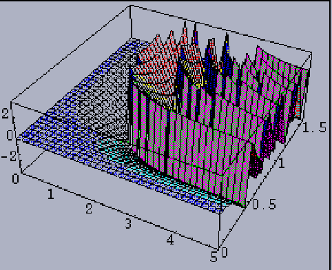
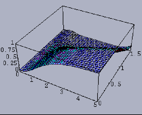
(In some of the later [computationally-intensive] figures in this section, it proved essentially necessary to omit the [otherwise obvious] axes labels, due to some quite distinct peculiarities of the graphics facilities for the local installation of MATHEMATICA on the more powerful workstations.)




V.2 Cross-comparisons of Uhlmann holonomy invariants


V.3 Eigenvalues of Uhlmann holonomy invariant for
To supplement our consideration above of the traces of various powers of the Uhlmann holonomy invariant (7), here we examine the eigenvalues themselves. (Both these traces and eigenvalues are themselves invariants, of course.) In Figs. 59 and 60 are shown the arguments of the dominant and subordinate eigenvalues of the holonomy invariant (7) for the case , and in Figs. 61 and 62, the corresponding absolute values.


In Figs. 63 and 64, we plot the arguments of the dominant and subordinate eigenvalues of the holonomy invariant (7) for the case and in Figs. 65 and 67, the absolute values of the two corresponding eigenvalues. The argument of the intermediate (in absolute value) one of the three eigenvalues appears to always be identically zero, that is, this intermediate eigenvalue is real (Fig. 66). It also appears numerically, on the basis of further analyses we have conducted, that this result is generalizable to the proposition that for odd , the central/most intermediate one (that is, the -th) of the eigenvalues is real. (Also, the centrally located diagonal entry of the holonomy invariant for odd appears to be real, in general.)


In Figs. 68-71, we show the arguments of the eigenvalues of the Uhlmann holonomy invariant (7) in the case . (The case proved more intractable in nature.) The third eigenvalue is simply real. In Figs. 72, 73, 75, 76 are shown the corresponding absolute values. In Fig. 74 is shown the value of the (real) intermediate eigenvalue.


VI Sjöqvist et al geometric phases for Gibbsian -level systems ()
In the approach of Sjóqvist et al [1] every pure state that diagonalizes the initial density matrix is parallel transported separately. By weighting the associated holonomy of each such pure state by the corresponding eigenvalues, we obtain the measure proposed in [1] “in the experimental context of quantum interferometry”. Since it is essentially trivial to obtain the pure states that diagonalize the initial (diagonal) -level Gibbsian density matrix and the associated eigenvalues, and since Uhlmann has presented the holonomy invariant (the trace of which is the Berry phase)
| (15) |
for the circular evolution of pure states, we can directly compute the Sjöqvist et al geometric phase () and visibility () for the -level Gibbsian density matrices. These are presented in Figs 77 to 86 and Figs. 87 to 96. The trace of the weighted (by the eigenvalues) sum of the holonomy invariants (15) for is
| (16) |
while for , it is
| (17) |
for ,
| (18) |
and for ,
| (19) |


VII Sjöqvist et al visibilities for Gibbsian -level systems ()


VIII Comparisons across Gibbsian -level systems of Sjöqvist et al geometric phases and visibilities
In Figs. 97-101, we display the direct counterparts of Figs. 21-25, but now based on the methodology [1] of Sjöqvist et al rather than Uhlmann. (We omit the counterpart of Fig. 26 because it appears to consist of essentially noise.)


IX Direct comparisons of Uhlmann and Sjöqvist et al results
In Fig. 102, we plot for the ratio of the Sjöqvist et al geometric phase (Fig. 81) to the Uhlmann geometric phase (Fig. 5), and in Fig. 103, the corresponding ratio for . In the next two figures (Figs. 104 and 105), we show the ratios of the associated visibililities.


X Summary
We have reported an in-depth study here of two different methodologies for determining geometric phases for mixed states [1, 2]. The analysis has been framed in terms of rotations (-orbits) of -level Gibbsian systems, as originally proposed by Uhlmann [3].
There are, of course, many features in these results. One of these is that the Sjöqvist et al geometric phases (sec. VI) appear to be less sensitive to the inverse temperature parameter () than do the Uhlmann geometric phases (sec. II).
In particular, we have found (sec. IV) that as the number of levels of the Gibbsian density matrices increases (in the sample we have studied) from to 11, the Uhlmann methodology often yields simple monotonic behavior. On the other hand, this seems to be largely absent using the Sjöqvist et al methodology (sec. VIII), which appears among other things to be sensitive to the bosonic (odd ) or fermionic (even ) character of the system under consideration,
It is certainly important to note that if one sets the parameter — given in (4) — equal to zero in the approach of Uhlmann (sec. I), the resulting holonomy invariant (7) is simply equal to times the holonomy invariant of Sjöqvist et al [1, eq. (15)]. This would appear to help to explain the added complexity of the plots of the Uhlmann geometric phases (sec. II) vis-á-vis those of the Sjöqvist et al plots (sec. VI).
We have found compelling numerical evidence that for odd the central (-th) of the eigenvalues (ordered in terms of absolute value) of the Uhlmann holonomy invariant (7) is always a real number (sec. V.3). (By the fundamental theorem of algebra, for odd , one of the eigenvalues must of course be real — since complex roots come in conjugate pairs — but clearly not necessarily the centrally located eigenvalue.) Also, the -entry of the Uhlmann holonomy invariant (7) is itself real, for odd . In terms of absolute values, the diagonal entries of the invariant (7) appear to be always monotonically decreasing from the (upper left) (1,1)-entry to the (lower right) ()-entry. (We note that the angular momentum operator — entering in our equations (2), (4) and (15) — itself has declining [real] diagonal entries, that is, .)
Acknowledgements.
I would like to express appreciation to the Institute for Theoretical Physics for computational support in this research.References
- [1] E. Sjöqvist, A. K. Pati, A. Ekert, J. S. Anandan, M. Ericsson, D. K. L. Oi and V. Vedral, Phys. Rev. Lett. 85, 2845 (2000).
- [2] A. Uhlmann, in Nonlinear, Dissipative, Irreversible Quantum Systems, edited by H.-D. Doebner, V. K. Dobrev and P. Nattermann, (Clausthal, 1994).
- [3] A. Uhlmann, in Symmetries in Science VI, edited by B. Gruber, (Plenum, New York, 1993), p. 741.
- [4] P. B. Slater, e-print, math-ph/0111014.
- [5] J. Dittmann and A. Uhlmann, J. Math. Phys. 40, 3246-67 (1999).
- [6] R. Jackiw, Intl. J. Mod. Phys. A 3, 285-297 (1989).