Some properties for the low-lying spectrum of the ferromagnetic, quantum XXZ spin system
By
Shannon L. Starr
B.A. University of California, Berkeley 1996
DISSERTATION
Submitted in partial satisfaction of the requirements for the degree of
DOCTOR OF PHILOSOPHY
in
MATHEMATICS
in the
OFFICE OF GRADUATE STUDIES
of the
UNIVERSITY OF CALIFORNIA
DAVIS
Approved:
Committee in Charge
2001
ACKNOWLEDGEMENTS
I wish to thank my advisor, Bruno Nachtergaele, who has been exceptionally patient and generous with his time. He has shared many ideas with me, as well as introduced me to the fascinating subject of quantum spin systems. Without him, none of this research would have been done. I would like to thank my other first collaborators, Pierluigi Contucci and Oscar Bolina, who also helped me to understand the XXZ model. I would like to thank Professors Janko Gravner, Albert Schwartz and Craig Tracy. All of them have been my teachers, and all have helped me get out of some tight spots in my research. I would like to thank Professors Kuperberg and Khovanov for taking time to teach me many things that I should know. I would like to thank Wolfgang Spitzer, for being a fellow researcher, as well as a teacher on many occasions. I would like to thank my friends in the math department for creating a stimulating environment, which seems to get better all the time. I would like to thank my family, which is too large to mention by name. They have always supported my education, and given me much needed reality checks. I especially thank: my sister Amy, for being my connection to the real world; my brother Jason, for being my connection to his world; my mother Susan, for loving me with no strings attached; and Carmeliza for so much, including putting up with my problems, without ever burdening me with hers. I would also like to thank Robyn, Heath and the Navasca family, who I think of as part of my own family. Finally I would like to thank the members of the band “Tool”, whose music has been a source of inspiration during many late nights of study.
This material is based on work supported by the National Science Foundation under Grant No. DMS0070774.
Abstract
We consider several aspects of the XXZ quantum spin system. These aspects are: existence of a spectral gap above infinite-volume ground states for arbitrary spin-S XXZ chains; description of droplet ground states for the XXZ Hamiltonian with up-spin boundary conditions; and a constructive proof of nonexistence of spectral gap above interface ground states in dimensions two and higher.
In Chapter 1 we introduce the XXZ spin system, list some background. We also give a complete summary of the rest of the paper.
In Chapter 2, we review some known results, including : the existence of interface ground states of the quantum XXZ model in all dimensions and for all values of spin [2], [26]; completeness of this list for ground states in one dimension [49], [37]; quantum group symmetry for the spin-, spin chain [55]; existence and exact calculation of nonvanishing spectral gap above infinite-volume ground states for the infinite spin-, spin chain [36].
In Chapter 3, we extend the result of [36] by proving the existence of a nonzero spectral gap in one-dimension for spins higher than . We show that the gap depends on the magnetization, , of the ground state through an even, -periodic function, which is the filling factor for one-dimensional interfaces. We give numerical estimates for the gap, and observe that the gap is maximized at some value of anisotropy strictly the totally anisotropic Ising model and the isotropic model. Based on our numerical evidence we observe that the gap of a spin-S chain grows like linearly with S, and we conjecture that the rescaled gap converges to a fixed function of , in the classical limit.
In Chapter 4, we introduce two models a one-dimensional quantum spin droplet. The first is a linear XXZ spin chain with up-spin boundary fields, and a pinning field, which is an external, negative magnetic field at a single site in the interior of the spin chain. For special choices of the boundary field and pinning field strengths the model admits frustration free ground states, which describe a droplet of down-spins centered at the pinned site, on a background sea of up-spins. We analyze the interfaces between the domains of up-spins and down-spins. We show that in the limit that the droplet grows to ifninity, the right-interface is a convex combination of kink ground states with discrete Gaussian weights. After this, we consider the droplet Hamiltonian without pinning fields, which is a more realistic model. We show that it also admits droplet ground states, which may be expressed as a mixture of states obtained by tensoring an antikink state on the left half of the spin chain to a kink state on the right half. We also prove that there is a spectral gap above these droplet ground states. Our proof uses a method of “cutting” and “pasting” spin chains which is based on finding intervals where the spin are all up or all down. Finally, we prove that the amplitude for dispersion relation of droplet state energy versus momentum is decaying exponentially with the droplets’ size. I.e., the droplets have a mass which grows exponentially with their size.
In Chapter 5, we reprove a known result, that there can be no spectral gap above infinite-volume interface ground states of the XXZ Hamiltonian in dimensions two and higher [35], [50]. The original proof was based on the Goldstone theorem, which applies because the interface states break -symmetry. Using similar ideas, we construct explicit excitations, and develop rigorous upper-bounds for the spectral gap. We show that in the thermodynamic limit the decay of the spectral gap is at least as fast as , where is the linear size of the interface.. Our technique shows that excitations which minimize energy are spin waves, constrained to the quantum interface. In the course of our proof we develop an equivalence of ensembles (EOE) result to show that canonical and grand canonical ground states of the XXZ model are equivalent on small subvolume.
Chapter 1 Introduction
The main subject of this thesis is the quantum XXZ spin system, which is a quantum spin system with Hamiltonian
| (1.0.1) |
defined on the domain , where is the usual -norm, and is the spin matrix for spin in the coordinate direction at site . is a number between 1 and . This is a deformation of the usual isotropic Heisenberg model, for which . At one has the Ising spin system, instead. This is a ferromagnetic model because of the overall factor in front of the sum.
Spin is the most fundamental purely quantum phenomena. It is connected to the Pauli exclusion principle via the celebrated spin-statistics theorem, which says that all integer-spin particles are bosons and all integer-plus-a-half spin particles are fermions (c.f. [64]). Since its discovery, spin has been the key to understanding magnetism, and it plays a part in many modern theories such as the BCS theory for superconductivity. There are several different types of magnetism, the most well-known being ferromagnetism, antiferromagnetism, and ferrimagnetism. The first quantum model proposed for ferromagnetism was Heisenberg’s model, in which electrons are tightly bound to atoms of some regular crystal. For each atom, the unpaired valence electrons’ spins add by the usual quantum rules for addition of angular momentum, i.e. one takes the tensor product of for each electron. Due to the short range of magnetic fields, one makes the approximation that each atom interacts only with its nearest neighbors. The interaction term is . Since the interaction is -invariant, one can decompose the spin of each atom into its irreducible components, and the Hamiltonian will block diagonalize in such a way that the different irreducibles, for a single atom, are not coupled. Consequently, the lowest energy state will be a state such that at each atom the spin falls in only one of the irreducible representations, in this way one usually considers only the model where each atom of the crystal is equipped with a single irreducible representation of . (One should also consider the orbital angular momentum of the electrons, but as can be calculated by the Einstein-de Haas experiment, for most atoms this is negligible in comparison to spin angular momentum. Also, for many atoms, iron being one, the interaction is not a direct exchange as we have indicated, but the product of two antiferromagnetic exchanges with some other atom, such as oxygen, which results in an effective direct exchange.) The Heisenberg model is thus
where represents the sites for the various atoms. The most basic model is a homogeneous magnet, i.e. all coupling constants are equal to a constant. This way, one arrives at the XXX model, which is a special case of the XXZ model, obtained by setting . This model is often simply called the Heisenberg model. Although it is apparently quite simple, it does describe some magnets surprisingly well. It also has subtle features, for example it is a longstanding open problem to prove that the isotropic Heisenberg ferromagnet model has a phase transition in dimensions three and higher, and to prove long range order for the ground state of the spin- model in dimension two. It is important to note the difference between the isotropic and the anisotropic model, here. For the XXZ model Tom Kennedy proved, in 1985, [34] that the low-temperature equilibrium states possess long range order in dimension two and higher if any anisotropy is present, i.e. for all .
A seemingly more complicated model of magnetism would allow, instead of the -symmetric exchange , an anisotropic exchange of the form
It turns out that for certain purposes this is actually an easier model to study. It is certainly physically relevant, because some materials do have anisotropic exchanges. Also, by introducing the more general Hamiltonian, one can gain insight into the original Heisenberg model, for example by observing the dependence of ground states, or low excitations on . For example, in the model we will study in this paper, , while . This is called the XXZ model. It turns out that in all dimensions one can write down some of the ground states of such a model, and in one-dimension it has been proved that the known list is complete [49], [37]. For one dimension, one also knows the complete list of ground states of the isotropic model [37]. But the two models differ in that for the XXZ model a spectral gap exists above the one-dimensional ground states [36]; whereas, for the XXX model, one can obtain arbitrarily low-energy excitations of the ground state by introducing spin-waves, which continuously rotate a spin through over a long interval. But for the XXZ model, the anisotropy damps these spin waves, because there is a high energy cost for deviation of the spin from alignment with the -axis. Therefore the anisotropic exchange results in more stable ground states, and in fact one can obtain a theory of domain walls on the basis of this alone. For the XXX model, one must assume crystal defects and impurities or surface effects via boundary conditions to account for domain walls. For the XXZ model, in the thermodynamic limit, domain walls exist as stable ground states. Also, as mentioned before, some properties, such as long range order in three dimensions, are known to exist for the XXZ model with , and expected for the XXX model, but still have not been proved. It is a tantalizing thought that one might be able to prove this by taking , although the non-commutativity of the thermodynamic limit with the limit precludes any obvious implementation of this idea.
The XXZ chain has been much studied in the field of exactly solvable models. The Heisenberg model was proposed by Heisenberg in 1929. In 1931, Hans Bethe proposed a method of solution which, in principle, solves not only of the XXX model, but also the XXZ model. Later, with the advent of the variational Yang-Yang equation, the Bethe ansatz was put on solid mathematical ground; however the proof is only valid for the antiferromagnet. Since its inception, the Bethe ansatz has become an industry of its own; c.f. the excellent text by Korepin, Bogoliubov, Izergin [41]. In general the XYZ chain
has been shown to be equivalent to a zero field, eight-vertex model by Baxter; c.f. [10]. The XXZ model is equivalent to a six-vertex model, also known as an ice-type model. Such models were solved by Lieb [44, 45, 46], who used properties of the XXZ model in his solution. Alcaraz et.al. [1] used the XXZ chain with imaginary boundary fields to determine critical exponents of the Ashkin-Teller and Potts models. More recently, Greg Kuperberg used the six-vertex model, and in particular a result of Korepin and Izergin, in his proof of the alternating sign matrix conjecture [42]. Even more recently, the number of ASM’s has shown up in the coefficients of eigenstates of the XXZ model for special values of , and has led to new conjectures [58], [9].
Having mentioned only a few of the many interesting results associated to the Bethe ansatz and the exact solvability of the XXZ model, we make clear that our results are entirely independent of the Bethe ansatz. There are two basic reasons for this. The first is that the solutions of the Bethe ansatz have been shown to be complete only for , i.e. th XXX model, by Babbit and Thomas [65], [6]. Despite efforts by Babbit and Gutkin [5], [27] to prove the analog for the XXZ model, their results are not complete, and only address excitations which are perturbations of the translation-invariant state . The subject of our work are non-translation invariant kink ground states. It seems that a rigorous result regarding the Bethe ansatz for excitations of kink ground states would be extremely difficult, due to the fact that a kink ground state has both an infinite number of up-spins and an infinite number of down-spins. The second reason for choosing not to use the Bethe ansatz is that the results of this thesis are not tenable by the Bethe ansatz, in any case. Even putting questions of rigor aside, the Bethe ansatz ceases to be a viable method for the XXZ chain with spin , or spin systems on lattices in dimensions . There are some integrable spin chains with spin greater than , for example those worked out by Babujian and Tsvelik [7], but the XXZ model for higher spin is not one of these. This rules out two of the results of this paper: a proof of non-vanishing spectral gap for spin chains with spin , and an upper-bound on the rate of vanishing for the spectral gap above interface states in dimensions two and higher. Our third result, is a quantum model spin droplets, as ground states of the XXZ model with positive boundary fields. We give approximate formulas for the entire list of ground states, in the limit that the number of down-spins becomes infinite. Our results remain valid for states with infinitely many down-spins and infinitely many up-spins, and therefore extracting useful information from the Bethe ansatz is almost certainly impossible.
For our purposes, more useful than the supposed complete solvability of the XXZ model, is the existence of a quantum group symmetry. In comparison to many of the results surrounding the Bethe ansatz, the quantum group symmetry was discovered fairly recently, it was first set down concretely for the XXZ model by Pasquier and Saleur in 1989 [55]. Originally discovered by Woronowicz [68, 67, 69, 70] a quantum group is a smooth deformation of a Lie group in the category of Hopf algebras, or in the version of Drinfel’d [20] and Jimbo [30] a smooth deformation of the universal enveloping algebra of a Lie algebra in the category of Hopf algebras. A quantum group possesses module structures which are very similar to those of Lie groups and Lie algebras. In particular there is a product, a coproduct, an identity, a coidentity, and an antipode. However, for quantum groups, neither the product or coproduct is generally commutative. The coproduct allows one to make a representation on the tensor product of any two representations. This is important for quantum spin chains, because the Hilbert space is naturally expressed as a large tensor product of two-dimensional irreps of . It turns out that the two-dimensional representations of the quantum group , for real values of , are equivalent to the two-dimensional irreps of (c.f. [32]). Thus, there is a natural representation on any ordered spin-, spin chain. The fundamental result of Pasquier and Saleur, and later Alcaraz, Salinas and Wreszinski, [2], was that for a particular value of , namely a solution of , the XXZ chain with special “kink” boundary conditions
actually commutes with the entire representation. This gives a system of commuting variables, and it stands that one can compute the eigenvalues of , by first finding the invariant subspaces of . At this level, the tool of the quantum group symmetry is exactly the same as the symmetry is for the XXX model. Moreover, there are analogous results, such as the ordering-of-energy levels result by Lieb and Mattis [48], which is apparently also true in the framework of -symmetric Hamiltonians. A notable use of the quantum group symmetry is Koma and Nachtergaele’s proof of the existence of a spectral gap above the infinite-volume ground state [36]. One drawback of the quantum group approach is that it cannot be extended to the infinite-volume Hamiltonian. I.e. at the present time there is no rigorously defined representation of on the algebra of quasilocal observables which commutes with the kink Hamiltonian. In fact by a work of Fannes, Nachtergaele and Werner [23], no such representation can exist. Still, there is enticing algebraic (as opposed to rigorous analytic), work by Jimbo and Miwa [29], which indicates that in the thermodynamic limit the antiferromagnet possesses a symmetry of the quantum affine algebra . For rigorous analytic results, the symmetry of the finite-volume spin chains is the most that is available, but is often quite useful.
There are several reasons for studying the XXZ ferromagnet, as opposed to say studying the antiferromagnet. The first, is that ferromagnets are abundant in nature, so there is hope of developing a theory with real physical significance. For some efforts in the direction of physical applications of the XXZ ferromagnet, see [39], [40]. We note that in terms of the most obvious physical features of the theory, more is already proved for the antiferromagnet than the ferromagnet, such as long range order in dimensions two and higher [33], owing to reflection positivity. For our type of analysis, the ferromagnet is more natural to study, since the kink states have a simple asymptotic structure, and the interface is exponentially localized. By avoiding the Bethe ansatz, we seek to provide direct physical arguments to explain the low-lying spectrum. Along these lines, more rigorous results have been proved for the ferromagnet (such as the complete list of ground states and existence of a spectral gap in one-dimension). Finally, for finite volumes, more is known about the ground states of the ferromagnet than the antiferromagnet. Even for the XXX model, there is no simple formula for th ground state of the antiferromagnet, the best that is available is the ordering of energy-levels result of Lieb and Mattis [48]. In contrast, for any choice of anisotropy , any spin , and in any dimension, one can write down the ground state of the ferromagnetic XXZ model. Thus the ferromagnetic model is more amenable to rigorous research, at least for a beginner. It would be an interesting point of further research to see what one can prove along the lines of spectral gaps, etc., for the antiferromagnet, but one which we leave open for now.
The outline of the thesis is as follows: In Chapter 2, we introduce some preliminaries about the XXZ spin chain. In chapter 3, we generalize a result on the existence of a spectral gap for the infinite-volume 1-d spin system, which had been proved for spin-, but which we show to be true for all spin , as well. In chapter 4, we present two models for spin droplets, with the property that the ground states have a domain of down spins surrounded on the left and the right by domains of up-spins (contrasted to the kink state which has just down-spins to the left and up-spins to the right). We show that in the limit that the size of the droplet goes to infinity, the ground states have a very simple form, and also possess a spectral gap above. In chapter 5, we reconsider an old theorem that the spectral gap above interface ground states must vanish in the infinite-volume limit in all dimensions greater than 1. We reprove the theorem, constructively, giving an upper-bound for the size of the gap which is of the order , where is the linear size of a plane parallel to the interface. We briefly summarize each of these chapters, now.
We begin in chapter 2 by stating some important facts, which are all already in the literature. First, we state a theorem due to Alcaraz, Salinas and Wreszinski [2] on the ground states for the ferromagnetic XXZ model in any dimension, and with any spin-S. They showed that with the kink boundary conditions one can write down a simple formula for the ground states. For spin- and in one-dimension, the formula is
| (1.0.2) |
To motivate the kink boundary conditions, we consider the classical (spin goes to infinity) model. After this detour, we return to the Alcaraz, Salinas & Wreszinski theorem, which we state in slightly more generality than its authors did, because we want to allow for graphs which are not subsets of . As far as proof goes, the generalization is trivial, but it is useful in Chapter 4, where one model for a droplet Hamiltonian is shown to be equivalent to a kink Hamiltonian on a different graph. The discovery of Alcaraz, Salinas and Wreszinski, and particularly the choice of kink boundary conditions, was motivated by the earlier discovery that the finite-volume XXZ Hamiltonian is actually invariant under the action of the quantum group . This was probably known at some level for some time in connection with the Bethe-ansatz solvability of the model, but was first stated concretely for the XXZ Hamiltonian, including the choice of boundary conditions for the quantum group symmetry, by Pasquier and Saleur in [55]. We give a brief introduction to quantum groups and in particular in chapter 2, immediately following the main theorem of Alcaraz, Salinas & Wreszinski. We demonstrate the main result of Pasquier and Saleur that the representation of commutes with the kink Hamiltonian.
After this, we give a brief review of the work of Gottstein and Werner, [26], which was done contemporaneously with and independently of [2]. Gottstein and Werner, like Alcaraz, Salinas & Wreszinski, determined the finite-volume ground states, though only for dimension-one and spin-. However, they did considerably more because they also discovered infinite-volume ground states. In fact they noted a key feature of both the finite- and infinite-volume ground states, which is that they are “frustration-free” meaning they minimize each of the translation invariant nearest-neighbor interactions, instead of simply minimizing the sum. This fact, which allows the definition of infinite volume ground states, also gives an explanation of why the same ground states work for dimensions greater than one and spins greater than (although Gottstein & Werner did not explicitly note the latter). In Gottstein and Werner’s work, in order to treat infinite-volume zero-energy (zero-energy = frustration-free) ground states, they constructed an entire theory of infinite-volume zero-energy states as states on the approximate inductive limit of finite-volume zero-energy observables. This theory is somewhat more complicated than the usual definition of states on the algebra of quasilocal observables, because whereas the local observable algebra always decomposes as for any , the same is not true of the local zero-energy observable algebra .
The Gottstein & Werner theory is a natural extension, and is most useful for the zero-energy observables with respect to the kink Hamiltonian. For this case, the approximate-inductive limit is shown to be a algebra, with a Hilbert-space representation for which the representations of all operators are normal. In fact even more is true, because the Hilbert space representation coincides with the GNS representation of all the infinite-volume kink ground states, and is also the Guichardet Hilbert space (synonymous with incomplete tensor product) of all quasilocal perturbations of the vector
| (1.0.3) |
Using their theory, Gottstein & Werner show that the complete list of infinite-volume, zero-energy ground states, w.r.t the kink interaction, consists of two translation invariant ground states defined by vectors and , as well as the infinite-volume kink states which they define
| (1.0.4) |
In later work, [49], Matsui showed that for the case , the zero energy ground states with respect to the kink and antikink interactions are the complete list of pure, infinite-volume ground-states. After this, Koma and Nachtergaele [37] gave a new proof of this fact; one which did not explicitly use the existence of a spectral gap above the ground states. In particular, their argument extends to the case , to show that the complete list of pure, infinite-volume ground states for the XXX model is the sphere of translation-invariant states.
In addition to giving the finishing argument for the complete list of ground states of the XXZ model, Koma and Nacthergaele also showed that there is a spectral gap above all the ground states [36] for the spin chain with spin equal to . In fact this work predates the complete list of ground states, they show that there is a spectral gap above all the zero-energy ground states, and the existence of the spectral gap was an implicit part of Matsui’s argument, though not Koma & Nachtergaele’s argument, for completeness of the ground states. Koma and Nachtergaele’s proof for the spectral gap is based upon showing that for finite-volumes the spectral gap is bounded in each sector of fixed magnetization, , uniformly in . In fact not only is the bound uniform, the spectral gap itself is a constant independent of . This remarkable fact owes to the quantum group symmetry. It is known that the ground states form the unique -dimensional irrep of in the tensor product . Koma and Nachtergaele prove a lemma which shows that the next lowest energy band is an -dimensional irrep. Therefore, the next lowest energy band intersects every sector, except , which are one-dimensional, hence exhausted by the ground state band. This shows that the gap is constant, independent of (for ), and it also shows that the band intersects the -dimensional sector for which ; i.e. the subspace of vectors with just one down-spin. It is a fact that in this sector, the Hamiltonian can be easily diagonalized by transfer matrix methods. In this way, Koma & Nachtergaele prove that for a finite-volume spin chain of length , the spectral gap is exactly equal to
They parlay the result for finite spin-chains into an equivalent result for infinite-volumes. For infinite-volumes the spectral gap above a particular ground state is defined in terms of the GNS representation as the smallest number for which
is valid for all strictly local observables . Koma & Nachtergaele show that the spectral gap above all the infinite-volume ground states is
Note that this does agrees with the known result that there is no spectral gap above the infinite-volume ground states for the XXX model.
In chapter 3 we generalize the result of Koma & Nachtergaele to show that for spins greater than , the spectral gap above any of the infinite-volume ground states is still nonvanishing. Unlike the original paper of Koma & Nachtergaele, we cannot exploit the quantum group symmetry, because it is nonexistent for spin-1 and higher. A related fact is that for spin-S, , the spectral gap ceases to be independent of for finite volumes. Instead one finds that for , the gap is approximately an even, -periodic function of . This is due to the dependence of the gap on the filling factor , which in the Ising limit, is the magnetization at the site separating all ’s to the left and all ’s to the right. One can show that the spectral gap for sectors with , is bounded below, uniformly in , and therefore that the gap above all the kink ground states is nonzero. Unlike Koma & Nachtergaele, the proof is existential, instead of constructive. Essentially, we use exponential localization of the interface to reduce the problem of low-energy perturbations to an equivalent problem in finite dimensions, where we know a spectral gap exists. The spectral gap exists in finite dimensions because the spectrum is discrete, but in the proof we do not demonstrate explicit bounds for the finite-dimensional spectral gap. This is the main difference between our result and the original result of Koma & Nachtergaele, since they give very clear lower bounds on the spectral gap in finite-dimensions. One can also bound from below the spectral gap above the translation-invariant ground states, by other, easier techniques. True to the lack of quantum-group symmetry, the gap above the translation-invariant ground states is quite different than the gap above the kink ground states. The gap above the translation-invariant ground states is , for all spins S. However, at least for the Ising limit, the gap of the kink ground states is exactly 1. For , the kink state gap is always lower than the translation-invariant gap (this is obvious because the kink states have large domains which look essentially translation-invariant, so that any low-energy perturbation to the translation-invariant ground states would also work for the kink ground state), but both grow linearly with S.
Although our proof of the spectral gap is not constructive, there is an important inequality used, which lends itself to a numerical approximation of the gap for finite volumes. The inequality gives lower bounds for the spectral gap of the full kink Hamiltonian, which is a matrix, in terms of the spectral gap of a Hamiltonian of much reduced size. Specifically the reduced matrix has shape , where is the number of partitions of with at most parts of size each at most . Here , which is typically on the order of . The partition number can be bounded by . If one fixes S and lets grow, to approximate the thermodynamic limit, then the new system becomes much smaller than the original one as becomes large. The determination of the lower-bound matrix uses the theory of symmetric functions. Empirically, the lower bounds seem to converge quickly as , much faster than the rate of convergence for the exact value of the spectral gap, as can be determined by Lanczös iteration. From these numerical lower bounds one can deduce a startling feature of the spectral gap, which is that for the spectral gap is not maximized at , the Ising limit, but at some nontrivial value of . In other words, in the vicinity of the Ising limit, decreasing the anisotropy leads to more stable ground states. In fact, comparison with Lanczös iteration for the full Hamiltonian, as well as perturbation theory for the full Hamiltonian, shows this feature to be true for . This is entirely different than the situation for . From this, one may guess that there is a semi-classical behavior (in the limit ) for the low-lying spectrum, which is possibly quite different than the low-lying spectrum for the spin- model. We give additional numerical evidence for this, although we provide no analytical proof of this fact. A reasonable argument is currently in the works, but will be published later as a separate result.
In chapter 4, we present two models for droplet states in a quantum spin system, and derive the ground states for both. For the second model, which is the more realistic of the two, we also demonstrate a spectral gap above the ground states. For classical spin systems, such as the Ising spin system, droplet states have an important role. For the Ising model, a droplet state can be defined to be the equilibrium state for the model with all -boundary conditions, in the canonical ensemble with a fixed density , and temperature in the range , in the thermodynamic limit. The need for an upper bound on the temperature is apparent: if the temperature is too high then one will have a disordered phase where every spin is a Bernoulli random variable, independent of every other spin, and with identical mean values . Dobrushin, Kotecký and Shlosman showed [19], that if is in the correct range, then the equilibrium state is a sum of translates of states characterized by two domains, one nearly all up-spins, one nearly all down-spins, separated by a contour whose shape is given by the Wulff construction. Thus a droplet in the sense we defined before matches the physical meaning of a droplet, as observed in condensation of crystals, and described by the phenomenological Wulff construction. Other notable work on this area of research for classical spin systems is [12], [11], [57], [59]. In particular, in [59], it is shown how the droplet states help to understand dynamical properties of non-equilibrium states, which is quite interesting since non-equilibrium statistical mechanics is a relatively open field.
While the progress for the classical model is impressive, almost nothing is known about the same problem for the quantum model. I.e., can one derive states described by Wulff droplets in dimensions two and higher starting from a quantum interaction instead of a classical interaction? This question will probably be open for some time, since currently, it is not even known what are all the interface ground states of the quantum XXZ model, in dimensions two and higher. In fact, even for the interface ground states which have been determined, one does not have a proof of the stability properties (see [51] for more on the current state of the problem). What can be done is to obtain a model for a one-dimensional droplet. A one-dimensional droplet state should have a domain of down-spins on a background of up-spins. Unlike, for the classical model, even at zero-temperature, there are quantum fluctuations. Therefore, the interesting aspect of the problem is in determining the nature of the quantum interfaces between the three domains, of all up-spins to the far left, all down-spins in the middle, and all up-spins to the far right. In analogy with the Ising model, one expects to obtain droplet states for the canonical ensemble with a particular choice of density of down-spins, with either periodic boundary conditions (i.e. spin ring) or with a boundary field favoring up-spins. We consider a non-periodic spin chain with boundary field , which does favor up-spins at the edge, and we are later able to deduce the results for a periodic spin chain. The choice of magnitude for the boundary field is important since we know is the energy of a kink interface.
As with the classical case, even without periodic boundary conditions, there is a recovered translation symmetry in the thermodynamic limit. To break this symmetry, we consider a toy model of a droplet with a pinning field at some site in the center of the spin chain, which has the effect of pinning the droplet of down-spins to be centered at that site. This is a toy model because one should not require anything as unphysical as a pinning field (although one may interpret such a field as the effect of an impurity) to demonstrate droplet states. Also, with the correct choice of amplitude for the pinning field, namely the field equals , the model becomes nothing more than an antikink Hamiltonian glued to a kink Hamiltonian. For such a simple model, we can give an explicit formula for the ground state. Then the main challenge is to extract from this formula the behavior of the quantum interfaces at the two edges of the down-spin droplet. This is done straightforwardly using explicit formulae obtained in Section 2.6.
In chapter 4, following the toy model, we present a real model for the spin droplet, without the unphysical pinning field. For this model we are able to show that the translation symmetry is recovered, and that for large droplets, the ground states are approximately equal to the sum of states which are a tensor product of an antikink on the left with a kink on the right. This shows the quantum interfaces for a spin droplet are the same as for a kink or antikink state. We also demonstrate a spectral gap above these states. For our results, we need the size of the droplet to become large, but there is no requirement on the density of down-spins. It can range from zero to one, as long as the absolute number of down-spins is large enough. The main technique for the proof is to make use of the spectral gap result of [36]. If we can find a region with nearly all down-spins, then we can decompose the droplet spin chain
into a sum of an antikink and a kink spin chain, and a two-site droplet spin chain
Then, using the spectral gap result of Koma & Nachtergaele, we can show that any low-energy state must be close to an antikink on sites and a kink on sites . In order to find an interval of nearly all down-spins, we introduce a lemma, which we call Corollary 4.6.3, which shows that for the droplet Hamiltonian, and in fact for any Hamiltonian which is a finite perturbation of the XXZ Hamiltonian, in any long-enough finite energy state, there exists an interval, such that the restriction of the state to that interval is close to a convex combination of the two states and . To obtain an interval where the restriction of the state is just , we use an induction argument on the number of down-spins. Since we do not assume the number of down-spins is a positive fraction of the total number of sites, the induction argument is a little technical. It mainly relies upon exact calculations which can be performed for the kink and antikink states, to determine the probabilities of finding intervals of all up-spins or all down-spins. A corollary of our result, is that for periodic spin chains, one has the same form for ground states: namely a kink state tensored to an antikink states. Also, if one considers the GNS representation for the translation invariant all-up state, then one can decompose the Hilbert space into a direct sum of sectors of given finite magnetization. Our results imply that in sectors where is large but finite, the lowest-energy states also look like a linear combination of states which can be described as an semi-infinite antikink-state tensored to a semi-infinite kink state. A surprising feature is that droplets of a given size, at different locations interact very weakly. In fact two droplets with their centers displaced just one unit, have an interaction on the order of , where is the number of down-spins in the droplet. This weak interaction leads to a very flat dispersion relation for droplet energy versus momentum. In other words, the mass of the individual droplets grows exponentially with the number of down-spins comprising the droplet.
In chapter 5 we consider the spectral gap above the interface ground state in dimensions two and higher. These ground states are the natural extension of the kink ground states given by Alcaraz, Salinas & Wreszinski. However, the behavior of the excitation spectrum in dimensions greater than one is much different than in one dimension. Specifically, there is a continuous symmetry of the XXZ Hamiltonian, realized as global rotations about the -axis. This symmetry, as well as translation symmetry, is broken in the ground state due to phase-locking. Thus by the Goldstone theorem, as implemented by [43], there are gapless excitations in dimensions two and higher. This is the argument for the vanishing of the spectral gap in dimensions two and higher given by Koma and Nachtergaele [38], and later by Matsui [50]. One point of interest in this result is that one does not know whether the interface ground states are stable to small thermal fluctuations in dimensions two and higher. In contrast, in one-dimensional quantum spin systems the KMS state is unique [4]. Hence the translation symmetry of the Hamiltonian is not broken. This means the unique KMS state in each sector is the translation-invariant state, which shows that kink states are not stable to thermal fluctuations. The nonexistence of a spectral gap, proved by such general schemes as the Goldstone theorem, does not completely illuminate the nature of the low-energy excitations. Are such excitations localized in space? Is the gap vanishing with a rate that depends on the dimension? Is the shape of the interface significantly changed by these low-lying excitations? How do the excitations depend on the anisotropy and the sector number? These are some of the questions which we answer.
Chapter 5 is broken into two parts, corresponding to two papers. The first paper shows what type of variational states one would use to obtain lowest-energy excitations of an interface ground state in the grand-canonical ensemble. In the grand-canonical ensemble, one does not separate out subspaces corresponding to different numbers of down-spins, as is done in the canonical ensemble. By allowing states with a fluctuating number of down-spins, one can obtain simpler expressions for the ground states. Specifically, the ground states can be parametrized by a continuous, real parameter, , which we call the chemical potential. Defining (in -dimensions), the ground state is
| (1.0.5) |
Since this is a simple-tensor product state, it has many properties resembling a classical state, including “independence” of spins at different sites (i.e. statistical independence of the spin observbles at different sites with respect to this state). By perturbing a single site of the ground state to yield a spin orthogonal to the the original spin of that site, one can produce an orthogonal state. The number of such excitations equals the number of sites in the domain . We explicitly consider the perturbation
which does produce an orthogonal state due to the fact that the coefficients of the up and down spin at each site are real. By considering the Hamiltonian acting on such a perturbation, one discovers that can have a low energy, but only if obeys strict relations in the direction. Imposing these restrictions still leaves freedom in the definition of in one plane perpendicular to the -direction. Thus has one degree of freedom reduced, but in dimensions two and higher, this still leaves at least one additional degree of freedom. The plane perpendicular to the -direction is the plane of the interface, which we will call . If the portion of intersecting the plane has diameter , and if we assume varies continuously over this region like for some smooth function on a continuous domain, then the leading-order contribution to the energy of is given by
times a constant depending on . ( also enters the definition of through the relations for in the direction. The interface of the grand-canonical ground state is localized about the “plane” , and the restriction of in the direction has the effect that the perturbation is also localized about this plane.) The norm of the state is equal to
times a constant depending on . Thus, taking the Rayleigh quotient, one has the variational formula for the eigenvalue problem of the Laplace operator on the plane . This is not surprising since it tells us that the lowest excitation is a multidimensional analog of a spin-wave on the plane of the interface.
The second part of chapter 5 is devoted to the same problem in the canonical ensemble. In fact this is the more rigorous approach, since in this framework one can produce excitations which are not only orthogonal to one ground state, but to them all. (More precisely there is only one ground state per sector of total spin, so an excitation which is entirely in one sector and orthogonal to the one ground state in its sector is automatically orthogonal to all other ground states in other sectors. The difficulty with the canonical ensemble is that the ground states do not have the simple form of (1.0.5), and so it is not so trivial to construct a class of perturbations which are genuinely orthogonal. There are two steps which allow one to bypass this obstacle. The first step, which is trivial but important, is to use the variational inequality. If is the unique ground state in the sector with down-spins, then the energy of the spectral gap in this sector is
| (1.0.6) |
This allows us to bound the spectral gap by considering non-orthogonal perturbations of the ground state. The second step is to reduce the calculation of certain local observables with respect to the canonical ensemble to the calculation of the same observables in the grand-canonical ensemble. This is done by proving an equivalence-of-ensembles result. More specifically, for small subdomains , the restriction of the state to the observable algebra , is close to a grand-canonical ground state. This can be understood easily enough: although the number of total down-spins in the volume is a fixed number, the number of down-spins in any subvolume is varying. If the subvolume is small enough, then the distribution of down-spins becomes exponential, with Gaussian corrections of lower-order, by a usual central limit theorem argument. In fact, the relevant quantity to estimate turns out to be for all values of near . One can evaluate exactly for each , due to the factorization property of the state. Moreover the states form an exponential generating function for the canonical ground states. So, alternatively to the central limit theorem, one can use Hayman’s method (c.f. [66]) to determine the distribution of down-spins. This allows for a more refined version of equivalence of ensembles which is proved in the last two sections. As well as demonstrating explicit upper-bounds for the spectral gap, which shows that the gap vanishes at least (and probably at most) as fast as , we show how the spectral gap depends on the sector number . It turns out that the most fundamental effect is due to the partial filling factor of the interface plane, due to having particle number which is not a perfect multiple of the size of a plane. This is elucidated in the paper. Also, we show how the gap depends on the anisotropy parameter : it depends through two functions of which measure the first and second moments for particle number in the one-dimensional grand-canonical ensemble. This is the subject of the appendix. Our estimates are only valid for . However, we point out that for , even in one-dimension there are gapless excitations due to spin-waves, and for , the 11-interface is degenerate with all the other interfaces with the same global geometry and equal perimeter. Our arguments rely on nondegeneracy of ground states for finite volumes, as well the Koma & Nachtergaele spectral gap result above the kink states in one dimension, and so it is natural to only consider in the range .
Chapter 2 Preliminaries
2.1 Definitions
The quantum XXZ spin chain is a mathematical model for magnetism at the level of atoms or ions in a crystal. This is purely a spin system, consequently, no issues of charge of the atoms enter into the XXZ model. There is no kinetic energy for the atoms; in fact, the atoms are fixed at sites of a subset of a discrete lattice. For our purposes, the only lattices we consider in detail are the -dimensional integer lattices . Physicists call these simple cubic lattices. The most sensible parameter range for is . Our results, however, are of two types, those true for , and those which are true for all .
By we will usually mean a subset of . It is the collection of sites for our spin system. Unless otherwise specified, will be a finite set; i.e. . The configuration space for the spin of a single site is the Hilbert space , and the Hilbert space for the entire spin system is . The subscript simply indicates which spin the Hilbert space describes. carries an action of . More precisely, it is a -dimensional irreducible representation. This is natural in the quantum theory of spin. A good reference for quantization of angular momentum is [21], a good mathematical treatment of the representation theory of is [60]. What is most important for us is that there is a set of three operators , and defined with respect to a basis by
and
where
For us this is the most convenient way to specify the representation of . We also define the spin-vector .
With this notation, the one-dimensional spin-S XXZ Hamiltonian is defined as
We assume . The Hamiltonian is obviously Hermitian. It is easy to see that it is also nonnegative: Indeed,
where is the Casimir operator for the representation of on , and in particular has eigenvalues for each . The Casimir operators and are identically because and are spin-S irreducible representations of . This means that has minimum eigenvalue equal to 0, when . The minimum eigenvalue of is bounded below by , and . So, in fact, each of the summands in is nonnegative.
There are vectors which minimize each pair interaction simultaneously, namely and . Here we have adopted the notation
For , these two vectors are the only absolute ground states because they are the only vectors which maximize every pair , simultaneously, and also maximize each . They are the vacuum states for and , respectively, in the -dimensional irreducible subrepresentation of . These two states are ground states in the thermodynamic limit, . Or, more accurately, there are states , in , where is the set of quasi-local observables and is the space of continuous linear functionals on , given by for any , and these two states are ground states. For the general framework of states in a quantum spin system see [16] or [61]. By definition, a state is a ground state iff
for all . Since and , it is trivial to check that for any , with . Since
it is clear that are infinite-volume ground states. The states are also pure states, which is to say extremal elements of the convex set of all normalized states. This is apparent from the definitions. However, they are not the only pure, infinite-volume ground states. The first natural question which arises about this Hamiltonian is
-
1. What is the complete list of pure, infinite-volume ground states?
A complete solution to this problem was eventually found by Koma and Nachtergaele in reference [37], although to place the problem in its proper perspective one should consider a number of other results, most notably [2] and [26]. In order to motivate the treatment of the quantum problem it is instructive to consider the classical model. It is important to note, however, that this was not the original motivation behind exact results for the ferromagnetic model. Historically, the Bethe ansatz and the quantum group symmetry played a much more active role in leading to the formula for the ground state of the XXZ model.
2.2 The Classical XXZ Model
The purpose in examining the classical XXZ model is to give an intuition for the quantum model, the ultimate goal being to find all the infinite-volume ground states. It is typically the case that one can obtain infinite-volume ground states by considering a sequence of finite-volume Hamiltonians with the “correct” boundary terms added. This is the case for the XXZ model, as will be shown in the next sections. In this section we try to “guess” the correct boundary conditions, of course with the caveat that having read the original papers [55], [2], [26] and [37], we know beforehand what the correct boundary conditions are. We treat the case of finite anisotropy, , separate from the infinitely anisotropic, or so-called Ising limit.
2.2.1 Finite Anistropy
To obtain the classical model, one formally takes . Thus, one scales
and in the limit , obtains
where is a unit vector for each . Actually, it is not the Hamiltonian itself which is well-defined in the limit, but rather the partition function associated to the Hamiltonian: c.f. [47]. Still, one may define a nonnegative functional on the space of all sequences by
Although this may take the value infinity, it is always well-defined, since all the summands are nonnegative. In spherical coordinates
where and . Then
It is clear that the choice of which minimizes is for some . Thus every minimum-energy state of is a planar rotation. With this assumption, we have
In order to have a minimum-energy state, should be extremal with respect to every . Hence
Defining , and using the angle addition law for tangent, gives
| (2.2.1) |
If we make the ansatz that for some , then we observe that , so drops from the equations, and we are left just with the condition
Definition 2.2.1
For let be the unique solution of the quadratic equation , i.e. . For , and for , .
Hence there are two one-parameter classes of solutions to (2.2.1): the so-called kink solution or , and the so-called antikink solution or . It may be preferable to write the solutions in terms of the original coordinates . The fact that is fixed means that the kink and antikink solutions are planar waves:
| (2.2.2) |
Then the wave is specified just by the sequence . While there is no simple linear recurrence for the , there is the next best thing, a linear-fractional recurrence relation:
| (2.2.3) |
where is a special value defined by
| (2.2.4) |
For these solutions to be valid, we must require , i.e. we exclude the case , which corresponds to the Ising limit. In the isotropic limit, , , all the solutions are translation-invariant with for any vector on the two-sphere. For there are still two translation-invariant ground states corresponding to , all up-spins, or , all down-spins. For any other choice of , we observe the behavior,
![[Uncaptioned image]](0106024v1/kink.png)
![[Uncaptioned image]](0106024v1/antikink.png)
So the profiles for are schematically as in the figure above.
We can calculate the energy stored by the kink and antikink states. The energy of the interaction between site and is
Defining
we have
Completing the square, we have
It is a straightforward calculation to see that for the kink state
So the energy of each interaction is
There is no need to calculate each interaction energy as a function of and because, since , the sum is a telescoping sum:
Thus we see that all kink states have the same ground state energy, independent of the choice of . Similarly, the energy of the antikink states is also .
Even though the energy of the kink states is higher than the energy of the translation-invariant states, it should be noted that both are ground states. The reason is that the translation-invariant ground states, , and the kink states are mutually singular (have no absolutely continuous part w.r.t. one another). To see this it is sufficient to observe that they differ at infinity. Since we will be interested in analyzing kink states for finite chains and their approach to the thermodynamic limit, it is useful to define a new Hamiltonian which differs from by only boundary terms, such that the kink states are absolute ground states. Thanks to our previous analysis, we know exactly how to do this, namely, add to each interaction the term . Or, in terms of the original variable ,
| (2.2.5) |
Note that because of the telescoping sum, this is only a boundary field, i.e.
The significance of this change is not only that the kink states now have energy equal to the all up- and all down-spin states: It is that the kink states now minimize each pair interaction separately, instead of simply minimizing the sum of all pair interactions together. Such states are called frustration-free ground states signifying that they are not “frustrated” on any bond. They play a very significant role in the classification of ground states for the quantum XXZ model, as we will see shortly.
2.2.2 “Ising-type” states
We can treat the Ising limit in entirely the same manner as above, except that we must be careful whenever we use . It is simpler and more instructive to treat the Ising limit directly, since in most circumstances one gains intuition for the XXZ model from the Ising model, and not the other way around. The Ising Hamiltonian is
and we can replace the unit vector with just its third component which we rename simply . We point out that this is not the Ising model, since, among other things is allowed to vary continuously between and . In the quantum model with , the Ising limit really does correspond to the Ising system. For higher S, the Ising limit is not an Ising model because the configuration space has cardinality . It is also not obviously a clock model or Potts model. The simplest way to think of it is as a Ising spin-ladder model. The Hamiltonian above can be rewritten
It is clear that this model is ferromagnetic in the strictest sense, i.e. all spins prefer to be aligned as much as possible in the direction. One might then, precipitately, guess that the only ground states are . This is incorrect, it is possible to change the boundary conditions at infinity to force a domain wall. Namely, for finite volumes , by adding a boundary field which forces an up-spin on one boundary and a down-spin on the other. In fact our kink Hamiltonian is sufficient. The ground states are then kink states centered at any point ,
as well as the translation-invariant states .

In fact there are more ground states than these. Observing that can be written as a sum of nearest neighbor interactions
we see that it is possible to have a frustration-free ground state with one spin, say at site , in any orientation as long as all the spins to the left of are aligned along the south-pole and all the spins to the right are aligned along the north-pole. Thus we have a family of solutions , given by
Of course . Also, note that
for any sequence . However, neither nor is a quasilocal perturbation of any state in the span of , just as in the case . A pictorial interpretation of the ground state space for the different kink models is shown in Figure 2.1: For the isotropic (XXX) model, all ground states are translation-invariant, with any choice of unit vector for all sites; for the XXZ model with , there is a continuous family of points obtained by specifying the spin at, say, the origin, and then choosing every other spin to have the same angle and azimuthal angle . For the Ising model, the kink states are just what we have described above.
Also, with respect to the pair interaction , the states are all frustration-free. Of course, one can also define Ising limit analogues of antikink states, and the results are parallel (or rather antiparallel) to those for kink states.
2.2.3 Higher dimensions
For statistical models one can not often solve exactly for physical properties in one dimension; it is even more unlikely to solve a model in two dimensions; and it is almost never the case that one can find exact data rigorously in three dimensions and higher. However, for the XXZ model with certain domain wall-boundary fields, one can solve for the ground states in all dimensions. The reason this is possible is that the one-dimensional ground states defined by equation (2.2.2) and (2.2.3) are frustration-free ground states. As long as one can minimize the energy of each bond separately, it is possible to add extra bonds and sites to the one-dimensional model, as long as one makes sure that the state defined on the new site minimizes the energy of the new bond. Of course there are consistency conditions which must be satisfied, and for example if there is a non-simply-connected loop of oriented bonds, as occurs in a spin ring, then the ground state will not have a simple closed form. (One can retain something reminiscent of frustration-free ground states for a spin ring by choosing to be an th root of unity. Then it is possible to have a state such that its energy with repect to each bond is zero. However in this case , so that the XY-plane is the easy plane, and the Hamiltonian is no longer nonnegative. The “frustration-free” state one obtains is then not a ground state, it lies somewhere in the middle of the spectrum.)
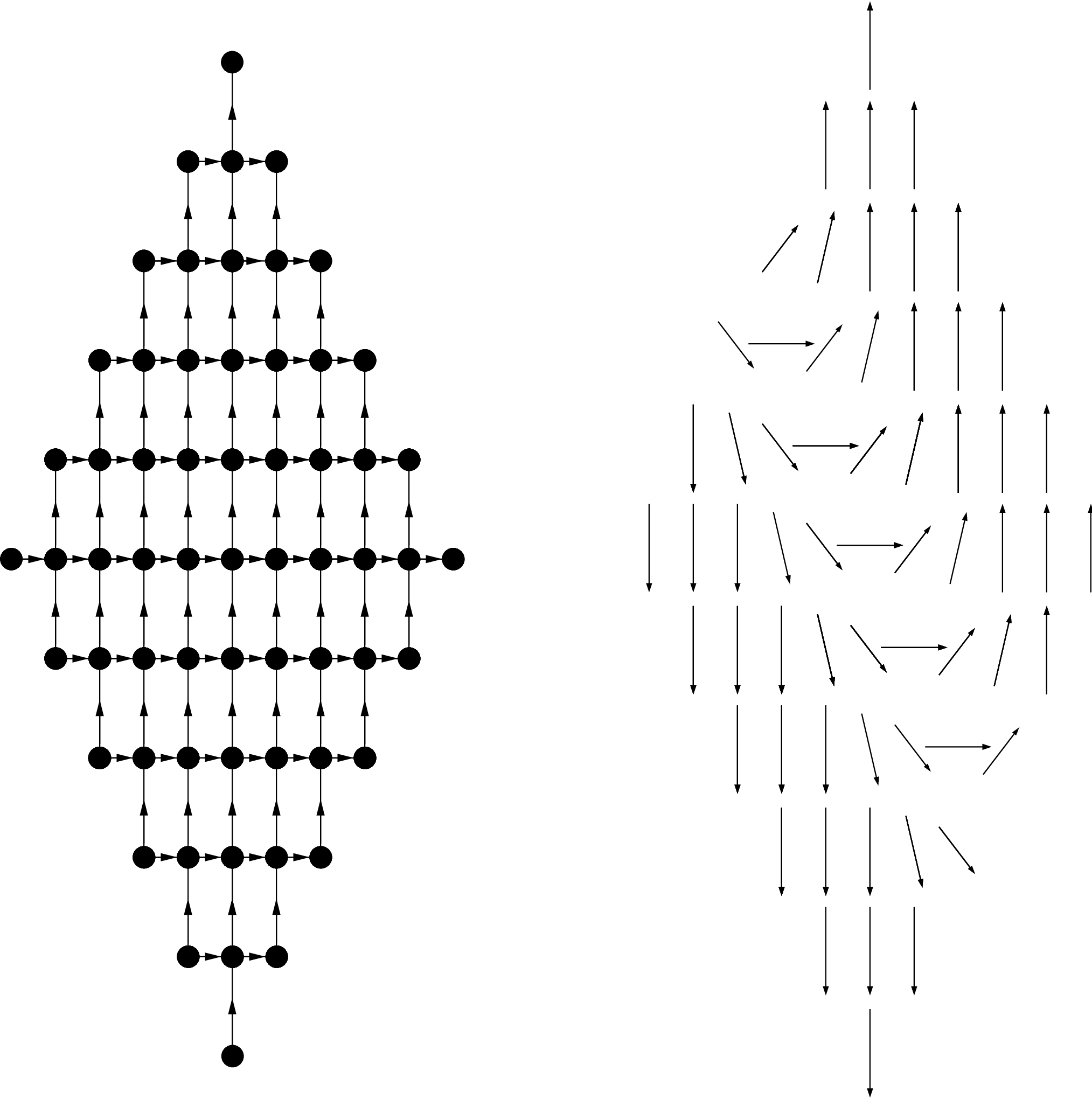
The specific condition for a frustration-free ground state of the classical system is the following. Suppose is a directed graph; so that a finite set, and a collection of ordered pairs of points from , which are usually called directed edges, but which we will call oriented bonds. We can then define the kink Hamiltonian on sequences by
One generally says that is connected if, for any pair , there is a finite sequence of points such that , and for all either or . We call such a sequence an unoriented path to distiguish it from the more common use of the word “path” wherein each must all be oriented bonds. We call the latter an oriented path. An oriented path is always also an unoriented path, but usually not vice-versa. For any two points , in a connected graph , there are typically many choices of unoriented paths. To construct a ground state for requires some consistency condition among all these unoriented paths. We define a height function to be a function with the property that
The consistency condition we require is that supports height functions, i.e. there exists some height function for . It is easy to see that if is connected and supports height functions, then any two height functions differ by a constant. It is also easy to see that if supports height functions then there is no closed, oriented path, i.e. no unoriented path such that and such that for each . In fact supports height functions iff for any closed, unoriented path, the path crosses the same number of oriented bonds going forward , , as it crosses going backward ,. With this characterization, it is obvious that if a directed graph supports a height function, then so does any subgraph. Similarly, the digraph supports height functions iff each of its maximal, connected subgraphs supports height functions.
With this terminology we have the following lemma
Lemma 2.2.2
(Classical XXZ model) If is connected and supports height functions, then for each real number satisfying there is a sequence with the property that
Moreover this sequence is uniquely determined by the number , up to scalar multiplication and a uniform rotation of every about the -axis by some angle . For , one has . For , any , and any height funtion , one can define the zero-energy state by equation (2.2.2) and
| (2.2.6) |
where is chosen to satisfy
Proof: To be a zero-energy state means that for every ,
This necessitates and
which in turn means
Clearly, if there exist and such that and for all , then for all oriented bonds , since . Conversely if for every oriented bond, then for any not necessarily an oriented bond, consideration of a connecting sequence leads us to the conclusion that and . Taking and for any , we have have the same condition as before. It can easily be seen that
So the lemma is proved once we observe that with fixed, the map
is a strictly decreasing, continuous map from onto .
This result is useful for example because one can make into a directed graph by defining
Then for any connected, finite subset , one can solve for the frustration-free ground states of . These ground states will have a -interface between down spins and up spins, because, up to adding a constant, the only choice for a height function is . A sketch of such an interface state for is shown in Figure 2.2.
There is a generalization of this technique which allows for different anistropies on bonds going in different directions. We delay this generalization to the spin- quantum model. We derive it there mostly because the formula for ground states of the XXZ model in dimensions higher than one is stated in [2] in just this generality.
2.3 The Quantum Kink Hamiltonian in Finite Volumes
For each choice of S, define the kink Hamiltonian
Note that we have placed the same boundary field as in the classical model, but scaled by S, so that every term in the Hamiltonian is homogeneous of degree . For , it is a simple calculation to verify
If then is the spin singlet, which is also the (unique up to scalar multiplication) antisymmetric tensor in . Thus, for ,
where is the transposition, and is the standard action defined by its image on simple tensors:
Thus, for the isotropic model, any ground state is invariant under the action of every nearest-neighbor transposition. Since the nearest-neighbor transpositions generate the entire symmetric group, this means the ground states of the isotropic model are exactly the symmetric tensors in the -fold tensor product. This is a standard result, which is related to the -invariance of the XXX Hamiltonian, because the subspace of symmetric tensors coincide with the heighest-weight, -dimensional, irreducible representation of in the tensor product .
2.3.1 Ground States
We will now state an important result of [2], which gives an analogue of the last paragraph for . The proof we provide is not exactly the same as the original proof of Alcaraz, Salinas and Wreszinski, or Gottstein and Werner [26]. This is mostly for pedagogical reasons. The discovery of ASW was originally related to the quantum group symmetry of the model, which was first explicitly pointed out in the paper [55]. Gottstein and Werner use generating functions to calculate the finite-volume ground states, which is fine, but one still needs a separate argument to show that all the ground states can be obtained in this way. We will take a different, but more direct, approach.
The result is analogous to Lemma 2.2.2, i.e. one can solve the model in all dimensions, provided there exists a height function for the directed graph of oriented bonds between nearest-neighbor pairs. In fact the formula from [2] is even more general, because it allows for different anisotropies in different directions. To put this in the framework of directed graphs that we already introduced, we need to expand our definitions slightly. Suppose is a finite set and are disjoint collections of ordered pairs from , which we will interpret as oriented bonds in different directions. Then, given numbers , we define the XXZ Hamiltonian with anisotropies by
We will say that is connected if is. We will call an unoriented path any sequence which is an unoriented path w.r.t. , and we define a generalized height function to be any function such that whenever . The existence of a generalized height function is equivalent to the property that any closed unoriented path traverses the same number of bonds of each type going forwards as going backwards:
One simple example of which supports generalized height functions is any finite subset of with the definitions . In this case, if is connected, then every generalized height function is defined by for some . Just as for height function, if is connected and supports generalized height functions, then all generalized height functions differ by a constant.
Theorem 2.3.1
(Alcaraz, Salinas, Wreszinski) If is a connected finite graph which supports a generalized height function , then for any choice , and S, the Hamiltonian
has a unique zero-energy state in every sector of total magnetization
Moreover, for a specified magnetization, the ground state is given by the simple formula
where , and each is the solution of .
Proof: We will first prove it for . In this case, we are guided by the argument at the beginning of the section which proves that the ground states of the XXX model are symmetric tensors. The key is to realize the ground states of the XXZ model as symmetric tensors, as well, but with a different choice of action of the symmetric group.
Let be the group of permutations of . The standard basis for is the set of all simple tensors of the form
where is a sequence of ’s and ’s. Let be the usual action defined by
We define a weight by
We define a new basis
and a new action by
With respect to the original basis,
Hence, if and if is the corresponding transpositon, then where acts on by
with and . Note that, restricting attention to and the representation of the two-element group , the symmetric tensors are
and the antisymmetric tensor is
Now we already know
from which it obviously follows that
Thus a state minimizes the interaction if and only if it is invariant under the action of . Hence a state is frustration-free, i.e. minimizes every interaction, if and only if it is invariant under every nearest-neighbor transposition. But it is well known that for a connected graph, , the nearest-neighbor transpositions generate the entire symmetric group . Hence, any state is frustration free iff it is invariant under the entire action of of . I.e. the frustration free states exactly coincide with the tensors which are symmetric with repsect to .
We know a formula for the symmetric states using the basis on which has the standard action:
This means that is defined in terms of the usual basis by
Mutliplying by a constant
one obtains the formula
This is the desired result for .

The result for higher spin systems follows by embedding any spin-S system with sites into a spin- spin system with sites. Specifically, define for be disjoint copies of . Let
For a single site , there is a natural way to identify with a subspace of , namely as the symmetric tensors. We define an action of on , wherein each copy acts by the usual permutation action on . Let be the projection onto the set of all vectors which are fixed by the entire action. Then by our previous consideration, this is precisely the projection onto . Then we see that
But also, the entire action of commutes with by the definitions of . (All bonds are allowed between any with for all and . Therefore, permuting the indices and does not change the sum.) Hence, also commutes with , and we see that the subspace of ground states of in is exactly equal to
But by its very definition as the symmetric tensors under the action of , one sees that the entire kernel of is contained in the range of . Hence the ground states of the spin-S model coincide with the ground states of . Writing these in terms of the natural basis for the spin-S representation gives
and this last formula is exactly what we want.
2.3.2 Quantum group symmetry
For this section we will consider only , and we will denote the representation of , instead as a representation of . The generators , , of the representation on actually define a representation of , not . But since is complex, we may as well consider the representations of . Indeed, it is most often more useful to work with the three operators which are the generators of the representation of , rather than the operators . Of course there is an obvious way to go back and forth, between complex representations of , and . But for now, we prefer .
A main feature of the isotropic (XXX) ferromagnet is that possesses a representation of , and moreover that this representation commutes with . By definition of our Hilbert space, each tensor factor is equipped with a representation of . There is then a canonical representation of on the tensor product , given by the generators
for . We reiterate that what we actually mean when we write is the operator
The reason we bring this up now is that we wish to examine for a moment the very basics of Lie algebra representations.
Defining to be the universal enveloping algebra, each representation of extends to a representation of . Moreover, there is a natural (unital) algebra structure on the tensor product , and the tensor product is most naturally a representation of this algebra. The way one passes from a module of to a module of (which is the same as a representation of ) is through the coproduct
(We are abusing notation since we use the symbol here for the coproduct, while elsewhere it refers to the anisotropy. Since the two uses of are so different, we trust the reader can tell which we mean from the context. In particular, for the rest of this section means coproduct: we use to parametrize anisotropy, here.) This is a homomorphism, as is checked through the calculation
The coproduct is coassociative, so that
is a commutative diagram, and the coproduct is even cocommutative so that , where is the switch-flip. By coassociativity, composing enough maps gives a well-defined algebra homomorphism as long as is an ordered set, and by cocommutativity, there is a well-defined homomorphism even if is not ordered. (This is a fundamental reason that one can analyze more easily than in dimensions higher than one.) The action of then gives the rule
as previously claimed.
The cocommutativity has the important consequence that since is invariant under the action of the permutation group generated by all the ’s, then for any , the subrepresentation
is a subspace of iff . Since the highest dimensional irrep equals for , we have a simple proof that the symmetric tensors comprise the highest dimensional irrep of in . This has the important consequence that the ground state space of is actually the highest dimmensional irrep of in . Another tell-tale sign of the coproduct is that by “forgetting” the coproduct we can obtain simple decomposition formulas. For example, the ground states of can be given by the formula
in which case one also has the identity
for any (where one interprets whenever is negative or greater than ).

Of course, since the XXX Hamiltonian commutes with the entire representation, not only is the ground state space equal to the highest dimensional irrep (as we have proved), but also every eigenspace for is a subrepresentation of , so that one can decompose into irreps of , such that each irrep is also an eigenspace of . We will now be able to interpret the symmetry in terms of computational evidence. We recall that a sector labelled by is the generalized eigenspace of the action of on with eigenvalue . We will call the sector . In terms of the sectors and eigenvectors of , we then have the following: In the sector , each eigenvector of is also an eigenvector of (the image of the Casimir operator of in ) with eigenvalue satisfying . If , then the raising operator maps the eigenvector to an eigenvector of with the same eigenvalue, but such that . Similarly if , then the lowering operator maps into an eigenvector with equal energy, and . What this means in terms of the spectrum, is that there are constant-energy bands sweeping through sectors with , corresponding to the irreducible representations in the Clebsch-Gordon decomposition of w.r.t. . This is clearly demonstrated in Figure 2.4.

The kink Hamiltonian for and is clearly not symmetric, which the interested reader may easily verify for himself. Therefore, it is something of a surprise that the distinctive structure of the spectrum which was just noted for the XXX model, whose explanation relied entirely on the symmetry, is still present in the kink Hamiltonian on a finite interval and for all . This is clearly demonstrated in Figure 2.5, where we have plotted the spectrum for a range of values between, and including, 1 and . We would obviously like an explanation for this. The answer is that while, for , the kink Hamiltonian is not invariant under the action of the universal enveloping algebra, , it is invariant under the action of the quantum universal enveloping algebra . In order for the last statement to make sense, we will now define , observing what are for us the most important features. This is not a comprehensive introduction to quantum groups. For that the reader is referred to the very clear reference [32]. This is the reference which we are copying.
A quantum group is defined as an abstraction of the structure of a Lie algebra. Given a Lie algebra one may form the universal enveloping algebra
Then is obviously a unital algebra, since it is the quotient of a unital algebra by a two-sided ideal . One defines a map , given by . Since the product on is associative, one is guaranteed that the following diagram commutes:
| (2.3.7) |
One also speaks of a map given by is mapped to the image of
which expresses the fact that the algebra is unital. Then
| (2.3.8) |
since the image of in the quotient is the left and right identity element. One can define a one-sided inverse of by taking the map given by for , and for any . This map is identically zero on so it factors through a homomorphism . Also, there is a map , which we have already define for , generated by , for any . One can check (in fact is encouraged to check) that the following diagrams commute
| (2.3.9) |
and
| (2.3.10) |
(Note that defining on determines uniquely on all of since is an algebra morphism. So, for example, from the fact that for any , we have that , for any , which forces , while as a second example
for any .) One can also check commutativity of the diagrams
which express the fact that the algebra structure given by and is compatible with the coalgebra structure given by and . Any linear space with linear maps , , and , satisfying equations (2.3.7)–(2.3.2) is called a bialgebra. There is one last piece of the puzzle before defining a Hopf algebra. Given two endomorphisms , we define the convolution , as the composition
(So for example, for , one has
while , and
for any .) An antipode of , if it exists, is by definition an endomorphism of , such that . (For , this means that and act as the identity on and annihilates for each .) One can check that the map which is an antihomorphism for any , and which is further determined by the rule for any , is an antipode. And the reader who is new to Hopf algebras is strongly encouraged to do so, at least by checking the value of the convolution on the elements , and . A Hopf algebra is by definition a bialgebra with an antipode .
Now our main example of a Lie algebra is . The Lie algebra of is a three-dimensional Lie algebra generated by , and , with
One definition of a quantum group is as a smooth deformation of – for some Lie algebra – in the category of Hopf algebras. The example which interests us is . We define to be the algebra generated by five elements , , , , and the relations
The parameter is allowed to be any nonzero complex number. For different from , and , one may reduce the number of generators by one by defining
and this is literally what one means by . However, it is important that is well-defined even for because then one finds
so that is really a deformation of . Of course, for , one already has a Hopf algebra structure on . For , one may define a Hopf algebra structure on by the definitions
and
although we will not verify this here.
It is a well-known result that for any complex number other than a root of unity the representation theory of is equivalent to the representation theory of . We paraphrase some definitions and theorems from Kassel: For any representation , and any nonzero one defines to be the eigenspace of with eigenvalue . If , then is called a weight, and is called a weight space. For any weight , a nonzero such that and is called a highest weight vector. For , and any , one may define an -dimensional module which is spanned by vectors with
where and
This is a simple module with highest weight vector of weight . Then, as proved in Kassel, one has the following results
Theorem 2.3.2
(Representation theory of ) Any finite-dimensional simple -module is isomorphic to for some choice of and . Any finite-dimensional -module is semisimple. One has
Denoting by , then for ,
We will now give some explicit representations of . Specifically, we will give a representation of on the vector space and show that is commutes with . For the purpose of the representation, we will not distinguish between the elements , , and and their images in . For concreteness let . Then
defines a representation. We define and instead of and as a matter of convention (because these are the operators which are defined in [36]). To prove that this is a representation we should check the relations. Evidently . Also,
Hence
which implies that
Finally, we calculate . Note that owing to the relations above . Let be the Heaviside function
Then
and
Note that if then
Thus
as required. One usually then defines the Casimir operator
with the result that on a irrep, the Casimir operator takes a constant value
Also, denoting the representation on by , , and , one can check by definition that for and ,
Note that in terms of the representation we have given it is easier to check that
In fact, this is obvious since
Next, we will show that the entire representation of commutes with . We already know that does. Hence and commute. Suppose , then
Hence
This is the ground state space. So the three-dimensional irrep corresponds to the ground state space. For the one-dimensional irrep, and must both annihilate everything. Thus we see that and do commute with for the case . Now we can use the coproduct and the fact that is a sum of translation-invariant, nearest-neighbor interactions to show that the entire representation of commutes with for every . Specifically, for any , and any , we have
Then obviously , and all commute with . And we have just shown that and commute with , because this is the case . So commutes with for every . A similar argument shows that commutes with every , as well. This symmetry explains the pictures of Figure 2.5, and gives a useful tool for comprehending the kink quantum spin system. We observe that we have not used the antipode, here, although it is an important feature of a Hopf algebra, since it allows one to do much more with the representation theory than one could do just with a bialgebra. (The antipode at the level of a Lie algebra is the same as the inverse at the level of the Lie Group . This is used, for example, to define a representation on given any representation on , by taking . In our case we did not need this piece of plethysm, just the fact that one could obtain a representation on , given representations on and .) Something else which will be useful later on is the Cartan automorphism on , which is an involution such that
This corresponds to the simulateneous reflection and spin-flip symmetry of the kink Hamiltonian. Either the reflection or the spin-flip symmetry alone takes the kink Hamiltonian to the antikink Hamiltonian. The fact that these two Hamiltonians are not equal is related to the fact that is not cocommutative.
2.4 The Infinite Volume Kink Hamiltonian
2.4.1 Zero-Energy Ground States
We return now to our original question, which is “What is the complete set of infinite volume ground states for the quantum XXZ model?” In [26], Gottstein and Werner realized that there are both finite and infinite-volume ground states which are actually frustration free. In fact, in finite volumes all ground states of the Hamiltonian with kink boundary conditions are frustration free.
For a finite volume ground state , being frustration free means that for all . Recall that for the infinite system a state is a bounded linear functional, , on the closed algebra of quasilocal observables . One observes that for any local observable , the derivation
is well-defined since the limit stabilizes (for ). A ground state is determined by the inequality
which must hold for all strictly local observables. This expresses the stability of a ground state to local perturbations. To be a zero energy ground state, must satisfy a more stringent condition. Specifically, if , where is a translation invariant pair interaction, ( is left translation, one unit,) then a zero-energy state is a state such that
for all . Of course being a zero energy state implies that is a ground state, because for any strictly local observable , restricted to the finite-dimensional algebra is a density matrix, in which case
where is the minimum eigenvalue of . Then
And, of course, the reverse is not necessarily true; i.e. it is generally false that all infinite-volume ground states are zero-energy. However in the case of the kink Hamiltonian, one may hope that it is true that the zero-energy ground states are the complete list of infinite-volume ground states, because all the finite-volume ground states are zero-energy. This turned out to be a correct prediction, on the part of Gottstein and Werner, although the proof, eventually given by [49] and [37] involved some real work beyond just the concept of zero-energy states.
The zero energy ground states give a nice intermediate step between the finite-volume ground states of the previous section, and the general infinite-volume ground states which one usually hopes to determine. It may be hoped that for some remaining open problems, such as all infinite-volume ground states of the XXZ chain in dimensions greater than one, that the zero-energy ground states would be a useful starting point. Gottstein and Werner found all the zero energy ground states for two spin chains, the XXZ and XXX, as well as connecting the notion of zero-energy ground states to some known results about Valence Bond Solid states. They did this by constructing a theory parallel to the usual theory of states on the quasilocal observable algebra, except now considering states on an algebra of zero-energy observables. For zero energy observables, one starts from the Hilbert subspace corresponding to the zero-energy vectors w.r.t. . The zero energy observables are then , the algebra of operators on . Note that the usual quasilocal observable algebra is defined as the inductive limit of local observable algebras , with the property that for , . This property is entirely due to the fact that , so that for one simply defines . But, for the zero-energy observables, it is not true that . E.g., although and are zero energy vectors of , is not a zero energy vector in . So, in order to define a zero-energy analog of the algebra of quasilocal observables, one needs a new inductive limit.
A first step in this process is the observation that the projection satsifies certain consistency conditions
| for all , and | ||||
| for all . |
This encodes the fact that for every finite volume the set of zero-energy states is nonempty, and that the restriction of a zero-energy state is a zero-energy state. For the case of a sum of translation-invariant, nearest-neighbor interactions, this is obvious because any restriction of a state on will clearly minimize every nearest neighbor interaction in (because it minimizes every nearest neighbor interaction in ). However these two simple assumptions are enough to guarantee that the set of infinite-volume zero-energy ground states is nonempty, which one can prove by weak- compactness. Gottstein and Werner use the notion of approximate inductive limits, which they review, in order to construct the Banach space of -convergent limits of local zero-energy observables, where
They then prove a theorem to show that , the space of zero-energy ground states on is isomorphic, via a direct construction to the space of ground states on the zero-energy observables. This means that a complete knowledge of the Hilbert spaces is sufficient to construct the zero-energy ground states, which are a priori defined in terms also of observables on the complementary Hilbert space . Unfortunately, the approximate inductive limit does not guarantee that is in fact a algebra, only that it is an order unit space. However, with the condition that for every -convergent nets , , the products is also -convergent, Gottstein and Werner prove that is a algebra.
Gottstein and Werner go on to consider Hilbert space representations of , analogous to the GNS construction. We will not repeat their results for the general case, but rather we state now the major application of their work, which is a Hilbert space representation of and the classification of for the special case of .
Theorem 2.4.1
(Gottstein & Werner)
As a convex set, the set of zero-energy states of the interaction is
isomorphic to the convex hull of the three quasi-equivalence classes:
(1) the set consisting only of the “all spins up” state
(2) the set consisting only of the “all spins down” state
(3) a set of “kink states”, which is isomorphic to the set of density matrices
on a separable Hilbert space. Each of these states converges in the
topology to (resp. ),
when shifted along the chain to right (resp. left) infinity.
We will not reproduce their proof. It is an analytic result, and it relies upon two important steps. The first is to realize that there is a simple formula for , a fact which can be traced straight back to the representation of on each , and particularly to the existence of the coproduct . The second is to examine the left and right asymptotics of any net of ground states, whose magnetic moments form a bounded net. This is the second statement of (3). In fact once this is known it is trivial to construct a Hilbert space representation of all kink states: it is simply the GNS Hilbert space of all quasilocal perturbations to the fiducial vector
Note that is not a ground state, nor a zero energy state. But there are many ground states, which can be labelled as the coefficients of the Laurent series
or directly by the definition
2.4.2 Complete List of Infinite-Volume Ground States
In [26], it was proved that all the zero-energy ground states are of the form given in the last section. But this does not asnwer the main question posed. It turns out, as was proved by Matsui in [49], and generalized (in particular, generalized to the XXX model, which was not possible with Matsui’s methods) by Koma and Nachtergaele in [37], that the zero-energy ground states are the complete list, not only for spin-, but for all spin. Of course, one must consider not just the kink interaction, but also the antikink interaction since these give the same Heisenberg dynamics on . Thus the translation invariant all up spins state , the translation invariant all down spins state , the kink states, and the antikink states, are the complete list of ground states for the infinite-volume XXZ model. We do not reproduce their proofs; however, we observe that a proof can easily be inferred from the methods and arguments of Chapter 4. This is not surprising, since the main ideas used in Chapter 4 are adaptations of techniques introduced in [37].
2.5 Spectral Gap
The next natural question after determining all the infinite-volume ground states, is to determine what the low-lying excitation looks like. The most fundamental question along these lines, is whether or not there exists a nonvanishing spectral gap in the thermodynamic limit, or if the spectral gap does vanish, what is its rate of vanishing?

In [36], Koma and Nachtergaele also provided a definite answer to that question by showing that for the one-dimensional spin-, there is a gap for any , which persists in the thermodynamic limit. It is the subject of Chapter 3 to verify that the same is true if one replaces spin- by spin-S for all . For dimensions greater than one, it is known, on the basis of general principles, that the spectral gap must vanish in the thermodynamic limit. In Chapter 5 we derive upper bounds for the spectral gap in dimensions two and higher, which shows that the spectral gap generally vanishes at least as rapidly as , where is the diameter of for the spin system. However, before any extensions of the spectral gap can be understood, one must know the basic result of [36]. We include a full outline of [36] here for two reasons: First, their result is concrete, precise, and important; Second, the method of proof is easy, and illustrates several tools of quantum statistical mechanics well, including the transfer matrix method, and quantum group symmetry. For this reason, it is especially good for students new to the XXZ model to see that proof.
It is known generally that for , there is no spectral gap in the thermodynamic limit. To prove this, it suffices to consider excitations of the all-up-spin state, since the ground states of the isotropic model are all unitarily equivalent (c.f. [37]). In this case, one can restrict attention to the “spin-wave” excitations. Although literally we should consider a linear spin chain of length , it is mathematically simpler to consider a periodic spin chain. Then the spin waves are
where is in the reciprocal lattice . Then, defining the periodic spin chain
where is identified with , we have
The actual ground state in this sector corresponds to . But an orthogonal excitation obtained by taking gives an energy of roughly . So the spectral gap decays at least as fast as for this spin chain. We should actually be asking what is the spectral gap for the XXX model with free boundary conditions. Koma and Nachtergaele calculated this, as part of their exact calculation of the spectral gap for the XXZ chain (since XXX is a special case of XXZ). It turns out that the spectral gap is exactly the same as for the periodic chain, except that one can take instead of . (For the free boundary conditions one can put a spin wave with wavelength equal to instead of .)
For one can ask whether the same procedure will work to produce arbitrarily low-energy excitations of the unique ground state in the sector of one overturned spin. The answer is no. Physically speaking, the anisotropy damps any such spin wave, because there is an energy cost for not having the spin aligned nearly fully along the spin-up or spin-down position. At a quantitative level, one may actually diagonalize the kink Hamiltonian restricted to this sector by using the transfer matrix method. Koma and Nachtergaele begin their analysis of the spectral gap by doing just this. We reproduce their analysis, now. One defines for each , the vector . Then an arbitrary vector in the sector of one overturned spin is given by the formula
for some sequence . It is easy to compute
So if is an eigenvector of , say , then
These conditions can be rewritten
for , and
Combining these conditions, one has
| (2.5.23) |
The matrix is called the transfer matrix for obvious reasons. It has eigenvalues
and eigenvectors
In terms of these, equation (2.5.23) can be rewritten
where
Or, since and are independent vectors
In case none of and this means
and taking into account the value of and , this gives . Hence where . For , this leads to
One can show that then the algebraic equations expressing the eigenvector are nonsingular, so that these are actually eigenvalues. Along with the ground state energy, which is zero, this gives all eigenvalues for the sector . Note the lowest excited energy in this sector is greater than .
Koma and Nachtergaele do not include this analysis just to show that spin waves fail to have a lower energy than . It is , in fact the basis of the calculation of the spectral gap for all sectors, using the quantum group symmetry to extend the results. We observe that any -dimensional irreducible representation of in the tensor product must intersect the sector with one downspin. Thus, to extend the spectral gap in the sector to the entire Hilbert space , it would suffice to show that for every choice of magnetization, , the lowest excited state actually lies in an -dimensional irreducible representation. In that case the eigenvector corresponding to the lowest excited energy can be raised by (i.e. the quantum group raising operator ) to a state in the sector with one downspin. Since commutes with , this means that the raised vector has the same energy as the lowest excited energy in the sector of magentization . But, as we have shown the raised vector, which is an eigenvector in other than the ground state, must have energy at least equal to . The argument is reminiscent of the ordering-of-eigenvalues theorem of Lieb and Mattis [48], except that here it is applied to the ferromagnet instead of the antiferromagnet. Koma and Nachtergaele prove that the main hypothesis is true, i.e. for the XXZ spin chain, as well as for any other spin chain with a quantum group symmetry, satisfying certain conditions, the lowest excitations occur in the -dimensional irreps of .
Define
for each . Then they prove the following lemma
Lemma 2.5.1
Consider an invariant spin-S ferromagnetic spin chain of sites with a nearest neighbor Hamiltonian , and for which the space of all ground states of a finite chain of sites is the irreducible representation of maximal spin (), for . Let denote the spectral gap of and let be as defined. If
for all , , then
Note that if , then this gives exactly what we want. An induction proof on then shows that for every , the spectral gap in each sector is .
One should note that Lemma 2.5.1 leads to a natural conjectured generalization. One knows, by the classification of the finite-volume ground states and the quantum group symmetry, that the ground states of the kink Hamiltonian comprise the unique highest-dimensional (-dimensional) irrep of in . By the lemma, one also knows that the second lowest energy levels correspond to a -dimensional irrep. Suppose one defines for each , to be the lowest energy of any irrep of in . (Since acts as a multiple of the Casimir operator on each irrep, we can speak of the energy of an irrep.) We know that for any other . Based on numerical evidence (some of which is included in Figure 2.5), we conjecture that whenever . To my knowledge, this conjecture was first formulated by Wolfgang Spitzer.
Since the spectral gap is nonvanishing in the limit , it is natural to suppose that there is a nonzero spectral gap above the infinite-volume ground states, as well. Koma and Nachtergaele prove that this is true, as well. To understand the slight subtlety of this statement it helps to know the actual definition of the spectral gap for infinite-volume ground states. This definition is closely related to the definition of a ground state, which we recall is that
for all strictly local observables . This means that no local perturbation of can lower the energy. The locally perturbed state is obtained here as . If one has a GNS representation of a ground state as a vector with zero energy, then for any strictly local observable , one has . The reason for this is that
where
is also a strictly local observable (for a finite range interaction). In fact the subspace of vectors is a core for all powers of . This means that the orthogonal complement to the ground state space is spanned (in the sense that the closure of the span equals the desired subspace) by the vectors . The reason for this is that is self-adjoint and annihilates all ground states. Thus, the infinite volume analog of the definition
is the definition: is the spectral gap above the ground state iff is the smallest number making the following inequality true for all strictly local observables ,
Koma and Nachtergaele prove that for any of the infinite volume ground states (, , kink states and antikink states), the spectral gap is equal to . We omit their proof; however, see Section 3.4, the proof of Theorem 3.2.3, for essentially the same argument.
2.6 Exact Calculations for Ground States Properties in One Dimension
Several calculations for the XXZ model can be carried out exactly due to known algebraic identities. We put these in two categories: those which use basic hypergeometric functions, which are the -analogues of hypergeometric functions; and those which use Gaussian polynomials, which are the -analogues of binomial coefficients. The two cases are distinguished by the choice of the lattice . If is infinite, i.e. or , then basic hypergeomtric functions may apply. If fo some , then the best results are obtained with Gaussian polynomials. It seems that the hypergeometric functions give better, i.e. more algebraically succinct, results than the Gaussian polynomials, which makes sense because for infinite there are no boundary effects, so that one can take advantage of the discrete translation symmetry of the Hamiltonian. We will time, and again, use exact formulas for finite volumes in the subsequent chapters, but here we would like to state and prove some simple results for the infinit-volume ground states of the XXZ model. It is hoped that this type of calculation, which uses standard identities from the theory of basic hypergeometric functions, may serve as a model for future exact calculations.
We recall the formula for the ground states bi-infinite lattice, . These are vectors in the incomplete tensor product , where
We define . Then the ground states themselves are defined by
| (2.6.24) |
for , and , where is the spin flip which sends each to , and is reflection which interchanges and for every . It is easier to handle the generating function for the ground states, rather than the ground states themselves. We define
with the observation that
| (2.6.25) |
We now begin calculations based on such states.
2.6.1 Application of basic hypergeometric functions
The hypergeometric functions are defined by
where and are natural numbers, and is the shifted factorial
They are ubiquitous in mathematical physics. Basic hypergeometric functions are functions of whose coefficients, instead of being rational numbers, are rational functions of another indeterminate . One defines the -shifted factorial by
For , one may also define the -shifted factorial for :
from which one has the alternative definition
The basic hypergeometric functions are
The standard reference for basic hypergeometric functions is [25]. It contains the proofs of all the identities stated in this section.
The first thing we would like to do is find a formula for
where is defined by (2.6.24). It is certainly easier to calculate
In fact, one immediately has the formula
We wish to extract the formulae for the norm of the ground states from the formula for the norm of their generating function. We recall that , where is an isometry of the incomplete tensor product. Thus for all . This can also be seen from the generating function since
| (2.6.26) |
Since
this does indeed show that . In a similar vein,
Thus
| (2.6.27) |
which implies
This implies
This is remarkable because it gives us the formula for the normalizations modulo one constant . To actually calculate requires the first identity from the theory of basic hypergeometric functions.
The binomial theorem
is the most basic identity in the theory of hypergeometric series. It has the -analogue
which was proved independently by Cauchy, Heine, and others. If we let , then
We observe that , while
Thus we have
Replacing by and by and , we obtain
Since is the constant term in this series we have
This series may be evaluated with the second main identity.
One may recall the Gauss summation formula
Heine’s -analogue is the following
If we set and take then the right hand side of the equation above becomes , and since
left hand side becomes
This means
Replacing by , again, we find
and hence
| (2.6.28) |
The next natural question one would ask is what is the magnetic profile of ? In other words, for each , what is the expectation
By the rotational symmetry about the -axis, we know a priori that . What remains is to calculate . Once again the formula for the generating function is quite trivial. Since is a simple tensor product, it is easy to calculate
We observe that
Now from its formula, we see that
and
Using these relations with (2.6.26) and (2.6.27), we can derive
and
From this we determine
This means that it suffices to calculate for .
We observe
This implies
For future reference we repeat
| (2.6.29) |
From this formidable looking series we can extract a simple question: What is
By this we mean, is there a simple product formula which equals the sum above? As far as we know, this question is not answered in [25]. This is related to (2.6.29) by the fact that
So the calculation of this term is the same as our simplified question, with and . The second term in (2.6.29) is also obtained by setting .
The answer to our question is not given by Heine’s -analogue of the Gauss summation formula, which states
But, if we define
then by Heine’s formula,
This allows the continued-product formula
I.e.
(By a similar argument, if we let
then we have
for all . For the special case that is a positive integer, this leads to a terminating series
where
is the Gaussian polynomial also called -binomial coefficient. Of course we are interested in the case , which is not terminating.)
We now observe that
But by a very simple calculation one may verify
where we have put a second to remind ourselves that we have replaced by in the definition of . This means
From this one may determine
From this formula, one can see the exact behavior of the magnetic profile, and particularly that the interface is exponentially localized. I.e. the third component of spin approaches and as one moves to the right or left of the interface, exponentially fast and with rate .
Chapter 3 The spectral gap for the 1d, Spin-S model :
3.1 Acknowledgements
The results of this section are due to Bruno Nachtergaele, Tohru Koma, and myself. More specifically, the proof of the existence of a nontrivial gap was originally done entirely by Nachtergaele and Koma for the case of , which I then generalized to . The numerical analysis of the spectral gap, using the lower bounds obtained by Koma and Nachtergaele’s proof, was carried out by me under the direction of Bruno Nachtergaele. I will also present other numerical results in support of conjectures made by Bruno Nachtergaele and myself.
3.2 Introduction
The purpose of this chapter is to prove the existence of a spectral gap above the infinite-volume ground states for the ferromagnetic XXZ chain for every spin . If , the spin-S XXZ Hamiltonian on the finite chain is
The operators are the spin-S matrices acting on the site . For the case we are considering, which is a ferromagnetic model with spin alignment preferred along the third axis, . We define another parameter to be the solution to the equation with the restriction that . It has been shown that the correct finite volume Hamiltonians for determining behavior above the infinite-volume ground states have a boundary field, with opposite direction on the opposite endpoints of . Precisely, the finite volume Hamiltonian we will consider is
| (3.2.1) |
It is important to note that the boundary terms can be included in a nearest neighbor interaction
We gather here a few facts from Chapter 2, which we will need for our current arguments. We will denote the finite-volume ground states by
| (3.2.2) |
This is the unique ground state of the kink Hamiltonian which is simultaneously an eigenvector of with eigenvalue . For spin-, we denote the GNS vectors for the infinite-volume kink ground states as
| (3.2.3) |
where
In [37], it was shown that the zero-energy states introduced by Gottstein & Werner are the complete list of ground states for . More generally, the following theorem is proved for arbitrary :
Theorem 3.2.1
(Koma & Nachtergaele) For the spin-S XXZ ferromagnetic chain with the anisotropic coupling , the following statements are valid: There are two translationally invariant pure ground states, namely and . Any pure infinite-volume ground state that is not translation invariant is either a kink, or an antikink ground state, belonging to the set described in [26].
In [36] the spectral gap for the finite-volume kink ground states in the case was calculated exactly. This was then used to obtain the spectral gap above the infinite-volume ground states.
Proposition 3.2.2
(Koma & Nachtergaele) For the invariant spin- ferromagnetic XXZ chain with and , one has
Above any of the infinite-volume ground states the spectral gap is
We recall that this formula is specific to , because it relies on the -symmetry of the spin- model. The quantum group symmetry is absent for all other choices of S. More specifically, for spin-, it is proved that the spectral gap is a constant independent of the sector, except that the spectral gap doesn’t exist in the all up-spin or all down-spin sector because these are each one-dimensional. In contrast, for , the spectral gap will not be the same in all sectors; instead it depends on the “filling factor” of . This means the spectral gap is an even, -periodic function of the sector, for sectors with , in the limit that . There are some general techniques for estimating the spectral gap for quantum spin systems in [22], [53], [52], none of which depend on the quantum group symmetry. These techniques do not seem to be directy applicable to the XXZ model for , or at least not more directly applicable than the argument which we present here.
The main theorem for this chapter is the following:
Theorem 3.2.3
For any half-integer , and any , there exists a nonvanishing spectral gap above all the infinite-volume ground states of the spin-S ferromagnetic XXZ model. Moreover, above the translation-invariant ground states the gap is exactly .
The proof relies upon the existence of a gap for , and the explicit formulas for the infinite-volume kink states. Part of the proof is a result which says that the gap for the XXZ Hamiltonian is bounded below by the gap of a Hamiltonian on a much reduced state space. In Section 3.5, we use this technique to develop numerical recipes for estimating the spectral gap, and present the results for .
3.3 Spin Ladder Representation
We wish to reduce the problem of calculating the spectral gap for , to a form where we can make use of Proposition 3.2.2. The way we do this is by replacing the spin-S chain with a spin- ladder with legs. This will have the advantage that we obtain lower bounds by disregarding some of the interactions in the spin ladder. By neglecting these bonds, the resulting spin system ceases to be equivalent to a spin-S spin chain. So the spin ladder representation is a key part of the proof.
The state space for the spin-S XXZ Hamiltonian is , where is equipped with an irreducible representation of . The representation can be rewritten as the heighest-weight irreducible representation in the tensor product of two-dimensional representations . The subscript is just a placeholder. We denote
The following diagram should help with the definition:
We denote the projection of onto by . Alternatively, this is the symmetrization projection defined by its action on simple tensors
This simply indicates the well-known fact that the highest-weight irreducible representation in a tensor product of two-dimensional representations of is the subspace of symmetric tensors. The subscript refers to the order of the tensor factors. We define . (Since is a commuting family, the order of the product does not matter.) Then the Hamiltonian can be recovered as
| (3.3.4) |
This is not technically the same operator since the displayed operator has a larger domain, but it is identically zero on , which is the orthogonal complement of in . The state space should be thought of as a spin ladder with legs defined by the state space , . The Hamiltonian acts on each of the legs separately, but in the legs are coupled through the conjugation by . Each acts on the rung , and connects the states on different legs.
We define the operators
and . By equation (3.3.4), the ground states of are the subset of ground states of in the range of . We define this subspace as . Then the spectral gap for is defined as
which, in view of (3.3.4), is equivalent to the formula
(Note that since , iff .)
We define the subspace to be the kernel of . Since each is actually a spin- XXZ Hamiltonian acting on the sites , we can use (3.2.2) to obtain
We define . We also define . By Proposition 3.2.2, it is clear that . Then we have the following estimate for .
Lemma 3.3.1
For any state , there exist two states , and such that
Moreover, if , we have
Proof: If , then also because
for any . Since , it is clear that there exist , with . By Proposition 3.2.2,
Using Cauchy-Schwarz, we estimate
and so
which proves the lemma.
We define
Then an immediate corollary is
Corollary 3.3.2
.
We can define a reduced Hamiltonian
on the Hilbert space . Then the corollary says . What is important to note is that while the original state space, is -dimensional, and the spin ladder state space is -dimensional, the reduced state space is only -dimensional. In addition, the reduced Hamiltonian is not more difficult to calculate (as is often the case), in fact it is easier because the basis states for have a simple formula, and are close to classical configurations of the Ising model. These benefits are the motivation for the approximations of Section 3.5, as well as for Theorem 3.2.3.
An important fact for each of the operators introduced in this section, is that they all commute with the total third component of spin
We define to be the th sector, i.e. the eigenspace of with eigenvalue . Then we define , and as the intersection of with , and , respectively. Note that is the one-dimensional space spanned by . In terms of the embedding , equation (3.2.2) becomes
There is one more piece of notation before we proceed. Given any , we define
| (3.3.5) |
Then
where .
Proposition 3.3.3
Given any sequence of triples , such that:
- •
is a finite interval,
- •
, and
- •
,
the following is true
3.4 Proof
Proof: (of Proposition 3.3.3) The proof is by contradiction. Thus we assume the existence of a sequence satisfying the hypotheses of the proposition, and also such that
| (3.4.6) |
We also assume, for convenience that each is normalized. By taking an appropriate subsequence, we can replace the in the formula above with a , and we assume this is done. Our method of proof will be to show that under the hypotheses given, and if in such a way that , then we can construct a limit state from the states with the property that it is an infinite-volume ground state and also is orthogonal to every infinite-volume ground state, clearly a contradiction. But in order to prove this we must first show that .
Lemma 3.4.1
If is a sequence satisfying the hypotheses of the proposition, and also equation (3.4.6) (with replaced by ), then .
Proof: Let us suppose first that
| (3.4.7) |
independent of . Then we can map to a state for every . But is a finite-dimensional Hilbert space, and the intersection of the range of with is exactly by equation (3.3.4). So it is clear that is strictly smaller than the identity operator on . Thus the conditions of the proposition along with (3.4.7) contradict (3.4.6). Now, in the general case, if does not converge to , then there is some such that infinitely often, and by taking the appropriate subsequence, we again have a contradiction. Therefore, it must be that .
By taking an appropriate subsequence, we may assume that . We assume this is done.
Lemma 3.4.2
If is a sequence satisfying the hypotheses of the proposition, and also equation (3.4.6) (with replaced by ), then .
Proof: We first assume
| (3.4.8) |
independent of in order to prove a contradiction. The proof is similar to the previous lemma, and essentially follows from the fact that for a finite-dimensional vector space the spectral gap is always positive. But this time the finiteness comes from , not , and we need to demonstrate that the subspaces actually converge to a single finite-dimensional space .
By the previous lemma, we know that . By taking a unitary transformation, if necessary, we assume that , with . Then we can write
We define two new vectors
where is defined as the tensor product of over , and
It is trivial to check that converges in norm to , as . Indeed, from our definition
From this it follows that
for each such that . Note that this is a finite set of multiindices , specifically, the cardinality is . Thus
which implies that as for every finite (because the same is true for by hypothesis). But also,
as . So, since , we have
Since the subspace is finite-dimensional, and all the have norm 1, there is a limit point of the sequence . This vector satisfies , for every finite , and . But, since the intersection of with is , the existence of such a vector is impossible. Thus we have a contradicition. So, does not equal any finite number infinitely often, and this implies .
Corollary 3.4.3
With the hypotheses of the last lemma, .
Proof: Follows from the last lemma and simultaneous spin-flip/reflection symmetry of .
By choosing a subsequence, if necessary, we can assume and . Also, by taking an appropriate subsequence, we can assume that all are equivalent modulo , i.e. that for and a number independent of . By taking a unitary transformation, we can assume . Since , it follows ; since , it follows . Let be the vector . Then every can be written uniquely as
with . (Recall that is the sum of the parts of , not the -norm.)
We observe that, for any fixed with , the sequence is bounded-in-norm by 1. Thus we may choose a convergent subsequence . By the Cantor diagonal trick we can, in fact, choose a subsequence such that converges for every (since the set of is countable). We assume this is done from the outset, so that for all . By Fatou’s lemma . But there is no guarantee at the outset that the opposite inequality holds, i.e. that . Next we will show that the coefficients are small whenever any part of is too large. This will allow the opposite inequality, and more.
Lemma 3.4.4
Proof: The proof of this fact is the most technical part of the paper. By hypothesis,
For any finite , and large enough , . In that case
So for every finite , . Now, for any , define to be the sum of all those terms for which , and let . We observe that
| (3.4.9) |
and
But also
unless , and if , then
by Cauchy-Schwarz. Therefore,
where
It is understood that we only take the supremum over those for which is defined. Thus actually has an implicit dependence on . But we claim that has a bound, independent of .
Claim 3.4.5
where is a universal constant depending only on (not on S, , or ).
Proof: (of Claim) Suppose that is a vector in such that is well-defined. Then for some ,
because , and for some other ,
because . We can estimate upwards by
where only symmetrizes in the two legs , . Now, obviously,
So
And
The estimate of the right-hand-side of the last display is the type of calculation which may be carried out directly from the definition (3.2.2). For details of these types of calculations see, for example, [13]. If , then the first of the two factors above is bounded by a universal constant (depending only on ) times , and the second factor is bounded by the same universal constant times . Absorbing , which is at most , into the universal constant-squared, we have the result.
Now, if we let
and if we let and , then by equation (3.4.9), we have
Solving for , we see that lies between , where
If we let stand for , instead, then we can take (because ). In this case, , where
Since as , we have
But since was arbitrary, we can take , to obtain
The reverse inequality is trivial, so the lemma is proved.
Here is an important application of the previous lemma:
Corollary 3.4.6
.
Proof: For any , we can find an such that
Since the set of all in the sum is finite, we see that
as . Thus
which implies
Since was arbitrary, the corollary follows.
We now define a new sequence of vectors
as well as the vector
Here, by we mean the tensor product of all the , , where is given by (3.2.3). It is trivial to check that for any fixed ,
as . (It is a similar computation to that done in Lemma 3.4.2.) Thus, for any finite , we have
where putting the superscript means the same thing as before, namely truncating the terms to those involving only with . By the lemma
Then following the argument in Corollary 3.4.6,
By its definition, is a ground state for for every finite , because each is. Also, by hypothesis, for any ,
Since , it is true that for any finite . Then by equation (3.3.4), is a ground state of for every finite interval . By Theorem 3.2.1, is a ground state. Since it is pure it is , , some kink,, or some antikink. The densely defined operator
distinguishes the different cases, and in particular all the infinite-volume kink states are eigenvectors for , with eigenvalue equal to . Similarly, each is an eigenvector with eigenvalue equal to . From this we see that .
But by hypothesis,
Another easy calculation is the fact that
So, this implies , which is clearly a contradiction. Therefore the Proposition is proved.
Proof: (of Theorem 3.2.3) We will first prove that there is a nonzero gap above the infinite-volume kink ground states. The same will then hold for the infinite-volume antikink states by symmetry. The gap above the translation invariant states will be calculated exactly, using a different technique.
Let be the largest number such that
for all finite , and all . By Corollary 3.3.2 and Proposition 3.3.3, . Then we claim is a lower bound for the spectral gap above any of the kink states . To prove this, it suffices to show that for any kink state , and any local observable ,
| (3.4.10) |
(This means that is greater than on its range in the GNS Hilbert space of all excitations of , since the vectors , , are a core for and all its powers.)
We observe that since is a limit of a sum of nearest-neighbor interactions, defining , . Thus,
and
Now define , and . Then restricted to is a density matrix , where each and . By the definition of , . So
This is equivalent to (3.4.10).
This proves the existence of a positive spectral gap above the kink and antikink states, although the value of has not been calculated. For the translation-invariant ground states, the spectral gap can actually be calculated by standard techniques. First we obtain a lower bound. For this, suppose that , where is the all-up state in the Guichardet Hilbert space , and . Then, (the boundary-field term is irrelevant since is asymptotically at ),
Now is diagonal in the basis
(where with finite support), and the lowest eigenvalue, for any state other than , is , which occurs whenever for some . This shows that .
To obtain the reverse inequality, let be the state when . We observe that
Hence
Let . Then
So,
which shows that , as well.
We observe that is not the exact value of above the infinite-volume kink/antikink states. To see this, consider the Ising limit . Then
is a ground state, and
is an excitation, which is orthogonal to every ground state. But the energy of the excitation is not , it is only 1.
3.5 Numerical Approximation
The decomposition of the spin-S spin chain into a spin- spin ladder was done just to prove the existence of a nonvanishing spectral gap. However, in view of Lemma 3.3.1, we can obtain a lower bound for the spectral gap of , in terms of the spectral gap of a much-reduced system. This is useful from the point-of-view of a numerical method because, while is sparse, even as a sparse matrix its dimension grows so quickly as a function of and S that it poses serious memory problems even for a moderately large spin chain such as , . On the other hand, by the lemma we can obtain a lower bound for in terms of , where is the largest eigenvalue, less than 1, of the operator (notation, )
The calculation of is possible because of the fact that the subspace has dimension , which is much less than the original dimension of which is .
One may ask whether the determination of a lower bound for the spectral gap for finite systems really tells us something important about the infinite system. We believe it does, since our main theorem shows that the spectral gap for the infinite-volume Hamiltonian is the finite, non-zero limit of the spectral gap for the finite systems.
The purpose of the next few paragraphs is to express the operator in the notation of symmetric functions. This is done partially just to obtain formulas for the matrix entries, which can then be evaluated numerically. But also, by this method we use the symmetries present to identify a large kernel for within . We will see that the combinatorial formulas that we bring in are very relevant to the problem, and arise naturally from direct analysis. We begin by defining an orthonormal system for . A classical configuration would be specified by stating for exactly which pairs there is a down spin. From this point-of-view it is useful to define to be the set of all matrices such that for all and , and such that the total number of ’s is . Then we define the state
These states form an orthonormal basis for . E.g.,
For each matrix we define a length- vector of the row sums, and a length- vector of the column sums:
Then equations (3.2.2) and (3.3.5), can be written as
| (3.5.11) |
From this, we see that is zero unless , and
We define
with the result that
| (3.5.12) |
where . We will come back to this equation later, to see how it can be made even simpler.
We can also write
which helps us to deduce
Therefore, combining this with (3.5.11),
Since
we then see that
| (3.5.13) |
To further simplify equations (3.5.12) and (3.5.13), we observe that for any and , , where
Moreover, for each orbit of under the action of , there is a unique vector such that . For such a , one defines the monomial symmetric function (in our case we consider it just as a function of variables )
where means equivalent modulo the action of . We define to be the subset of consisting of those such that and . They are called the partitions. If are the partitions such that , modulo the action of on , then equation (3.5.12) can be rewritten as
| (3.5.14) |
and equation (3.5.13) can be written
| (3.5.15) |
It so happens that is difficult, or at least messy, to calculate, particularly when has many nonzero parts. In order to fix this difficulty, we bring in the elementary symmetric functions. For , define
where , and for define
These are the elementary symmetric functions (restricted to variables). Two important properties of the elementary symmetric functions are
| (3.5.16) | |||
| (3.5.17) |
The second formula involves the well-known Gaussian polynomials
Both of these formulas are proved in Richard Stanley’s book [62]. With these formulas, equation (3.5.14) can be rewritten as
| (3.5.18) |
This simple formula can also be determined by other means.
For the matrix elements, we still seem to be stuck with the calculation of . We can get around this by defining
It is easy to convince oneself that the matrix elements are also integers, because has the triangularity property that unless , where refers to dominance order. This fact is also proved in [62]. Since the inverse of an upper-triangular matrix with integer components is also upper-triangular with integer components, we see that is always an integer, and the integer is 0 unless . Then we see that
Along with the triangularity properties of
this last formula can be used to rewrite equation (3.5.15) as
| (3.5.19) |
This is compared with
| (3.5.20) |
which we already derived.
We observe the fact that only depends on the orbit of and w.r.t. the action of . We define the subspace
which has dimension
Then cokernel of intersects in the single-dimensional subspace spanned by the element
Then, from (3.5.20),
while, from (3.5.19)
Thus, computing the normalized matrix entries of , we have
| (3.5.21) |
where
One aspect of this formula is that a certain part of it is totally independent of the value of . We may define
so that
| (3.5.22) |
One advantage of is that it stabilizes under . I.e. if and are each large enough that , and are in as well as , then the value of agrees for both choices of or . Also, the numbers have a certain translation invariance. Specifically, adding one to each part of , and (i.e. , for , etc.) does not change the value of , for large enough. Also, the leading-order behavior in is easy to see, since
Define to be the set of all partitions of . If one fixes , and , then taking yields
This is only true for strictly less than 1. However, for such , this gives a lower bound for the finitely magnetized spin chain on the half-infinite lattice :
| (3.5.23) |
which is defined for all .
This is almost of the form of a perturbation series, were it not for the -shifted factorials appearing in the formula. In fact, there is a way to eliminate these last remnants of -combinatorics, but at the expense of exchanging the finite matrices listed above for infinite matrices. The way to do this is to take a sequence of spin chains with and , but such that for all and , and such that . This is natural, anyway because it is by this limit that one obtains a state on the bi-infinite spin chain . Define to be the set of “signed partitions” or in other words just all sequences of integers such that such that . If one takes for , then as , one can take , etc. Then one obtains
| (3.5.24) |
Note that is well-defined due to the translation-invariance of with respect to its arguments. The -shifted factorials all approach in the limit , so their ratio cancels out. Again, this is only the case for strictly less than 1.
In the last two paragraphs we have taken limits, without commenting on whether it is valid to do so. Nor will we provide any attempt at rigorous justification to these procedures. The reason for our laziness is this: the entire point of this analysis is to obtain a simple model from which we can extract lower-bounds, which requires numerical computation, for the original model, which is the XXZ spin chain. We were, and are, interested in obtaining data from these lower-bounds, which hopefully leads us to make conjectures about the original model. It may in fact be easier to prove the conjectures for the XXZ model directly, rather than for the lower-bounds. Some of the conjectures will be presented in section 3.7. We have already begun work on the proofs, and our results will be reported in a later paper. We don’t want to undercut the importance of the lower bound derived in this section. It has two important roles. One is that it is the best, i.e. most efficient, numerical tool we have for looking at the low spectrum of the XXZ spin chain for larger values of S, so far. The second is that it has an interesting definition in terms of representations of quantum groups. We present this now.
3.5.1 Interpretation in terms of representations of quantum groups
We observe the following interpretation for the spectrum of . We started by considering a spin ladder, which is really nothing more than an array of 2-dimensional irreps of , . Of course, the 2-dimensional representations of are identical to the 2-dimensional representation of . So we can also think of our spin ladder as an array of 2 dimensional representations of . We define two sets of projectors. For each , we define to be the projection onto the top-dimensional irrep in the representation . For each , we define to be the projection onto the top-dimensional irrep in the representation . Then we ask for the spectrum of the operator
There are eigenvectors with eigenvalue 1, which correspond to the ground states of the spin-chain, which can also be interpreted as the totally symmetric states with respect to some representation of the symmetric group . (See Section 2.3.1 for more details.) The operator can be block diagonalized according to the eigenvalues of , which is well-defined since the image of is the same whether we consider a representation of or . Then in each sector there is a unique next-highest eigenvalue, and we write this as . Here is the eigenvalue of which lies between and . The matrix defined in equation (3.5.24) corresponds to the limit of as with fixed. For the special case that , the question is entirely in terms of representations of , but we note that we expect that as with fixed . For other values of , this is not the anticipated behavior. For example, for and , we know that the answer is , regardless of . The gap, , of the original spin chain is related to by . An interesting limit is obtained by first taking , and then taking . This is the classical limit of the spectral gap in the infinite-volume model (thermodynamic limit).
3.6 Numerical data
We present the results of our numerical experiments, now. We begin by looking at the results of the lower bounds estimates. For these estimates we considered the rigorous lower bounds obtained by equation (3.5.22). More specifically, fixing a sector with, down spins, we looked at the highest two eigenvalues of the matrix determined by equation (3.5.22) in that sector. This can be related to the spectral gap of the XXZ spin chain for the finite volume by corollary 3.3.2. Since we expect the behavior to be nearly translation invariant for large enough (i.e. in the limit that we expect the system to be entirely translation invariant, taking the sector defined by should not change the gap), we only considered . Moreover, since we expect the system to be invariant under simultaneous spin-flip and reflection of the spin chain, we can map into . Therefore, we only conisdered . Also, for obvious reason we did not begin with , but with . See Figures 3.1, 3.2, 3.3. It appears from the figures that in the sectors determined by , as one takes , then approaches the functional form . In this case, one would have the lower bound for equal to . This means that the lower bound for the gap scales with S as S, and that . This curve is significant because it has its maximum at a point other than the Ising limit, specifically at , i.e. .


To verify some of the results we calculated the real spectral gap for the XXZ spin chain for some small values of S and using Lanczös iteration. See Figure 3.4. This should give a very accurate answer, i.e. the numerical error is very low. Unfortunately, the finite-size effects are more significant for the full XXZ spin chain than for the lower bound, which appears to converge very rapidly in . For example, the Lanczös results at are certainly not the same as for , because then we expect at . It is well-known that there are gapless excitations, spin-waves, for the isotropic model in infinite-volume.

3.6.1 Perturbation Series about Ising Limit
We wish to perform a perturbation analysis for the first excited energy in the small parameter about the Ising limit . We write
Before proceeding, we note that with our choice of normalizations, is symmetric about . The reason for this is that can be mapped unitarily to via conjugation by the unitary operator
Thus we expect that the spectral gap has always either a local maximum or a local minimum at the point . In order to find which one, we perform second-order perturbation theory. We ignore the questions of degeneracy of the excited state for the moment, i.e. we begin by assuming that the excited state is nondegenerate. In a sector with , and , the ground state of the Ising limit is . The first excited state is
which has energy . First order perturbation theory yields
which implies
But because is an eigenstate of every . So . This then implies that
It is straightforward to calculate
Similarly, it is easy to calculate
By second-order perturbation theory, we obtain
From our calculations, this gives
For , one can obtain the value of by the previous formula, substituting for . For and , there are two degenerate eigenvectors with first excited energy equal to . One can easily carry out the degenerate perturbation theory to obtain the second order correction to the spectral gap.
A short table of values for some small values of S is given:
The blank entry in , is due to the fact that the excited state is infinitely degenerate: It is
or
This is the only value of other than which is infinitely degenerate. In the Ising limit, the minimum gap occurs for . One can see from the table above that for and , the gap is concave up at . Thus, for finite volumes, the minimum gap attains its maximum value for some other than 0, i.e. in some neighborhood of the Ising limit, as one increases the anisotropy, , the spectral gap actually raises. The perturbation theory does not prove that in the thermodynamic limit the gap is still maximized at some value other than , since it is possible this maximum value becomes smaller and smaller as . However, one can carry the perturbation series to higher than second order. We have calculated the perturbation series to 14th order for . The results are plotted in Figure 3.5. Unfortunately the perturbation series does not have radius of convergence equal to 1. In fact the radius of convergence is apparently approximately . One can see from these pictures that the maximum gap appears to occur for , as well, and the maximum gap seems to grow as a linear function of S.

3.7 Conjectures
Based on the numerical evidence, we make the following conjectures.
Conjecture 3.7.1
Denoting the lower bound for the spectral gap by , scales linearly with S, and the functional dependence on is
We also have strong evidence that the true spectral gap scales with S and that there is some curve , with maximum strictly between and such that
3.8 Matlab and Mathematica Notebooks
Source code for these two scripts is available on the arXiv. [63]
Matlab Notebook for Lanczos Iteration
This program defines the XXZ Hamiltonian with special boundary fields
%Also called the "Kink" Hamiltonian
%It restricts to the sector specified by the number "downspins" of down spins
%Using the differential equation for the first excited state as a function of Delta^(-1):
%$ h(x,y) = - S^3_x S^3_y - \Delta^{-1} (S^1_x S^1_y + S^2_x S^2_y)
% + A(Delta) (S_x^3 - S_y^3) $
%$ \frac{\partial h}{\partial \Delta^{-1}} = - (S^1_x S^1_y + S^2_x S^2_y) \\
% + \frac{\partial A(\Delta)}{\partial \Delta^{-1}} (S_x^3 - S_y^3) $
% we solve the first excited energy level as a function of Delta^(-1).
%Performs a linear-solve method "bicg" : biconjugae gradient.
dq = 0.005 %Step-size for anisotropy parameter
L = 4; %Spin chain length
J = 3/2; %Spin-dimension
downspins = floor(J*L)-1; %Number of downspins : sector
N = 2*J+1 %Dimension of single-site Hilbert space
S3 = sparse(1:N,1:N,J-(0:2*J),N,N); %Spin-J, spin matrix about e3 axis
Splus = sparse(N,N); %Initialization of spin-raising operator
for j=0:(2*J-1)
Splus = Splus + sparse(2*J-j,2*J-j+1,sqrt((2*J-j)*(j+1)),N,N);
end
Sminus = transpose(Splus); %Spin-lowering operator
S1 = (Splus + Sminus)/2; %Spin matrix about e1 axis
S2 = (Splus - Sminus)/(2*i); %Spin matrix about e2 axis
%IsingNN = Ising Nearest neighbor interaction S3(x)*S3(x)
IsingNN = kron(S3,S3);
%HopNN = Spin-hopping interaction = Splus(x)*Sminu(x+1) + Sminus(x)*Splux(x+1)
HopNN = - kron(Splus,Sminus) - kron(Sminus,Splus);
%IsingH = Ising Hamiltonian
IsingH = sparse(N^L,N^L);
for x=1:(L-1)
IsingH = IsingH + kron(eye(N^(x-1)),kron(IsingNN,eye(N^(L-1-x))));
end
%HopH = Hopping Hamiltonian
HopH = sparse(N^L,N^L);
for x=1:(L-1)
HopH = HopH + kron(eye(N^(x-1)),kron(HopNN,eye(N^(L-1-x))));
end
%BdryH = Boundary-field terms
BdryH = kron(S3,eye(N^(L-1))) - kron(eye(N^(L-1)),S3);
%S3tot = total third-component of spin operator
S3tot = sparse(N^L,N^L);
for x=1:L,
S3tot = S3tot + kron(speye(N^(x-1)),kron(S3,speye(N^(L-x))));
end
%We now define the projection to the sector specified by
% S3tot = (J*L-downspins)
Proj = speye(N^L);
for n=0:(2*J*L)
if ne(n,downspins),
Proj = Proj*(S3tot - (J*L-n)*speye(N^L))/(n-downspins);
end;
end;
%Proj is the orthogonal projection onto sector with specified number
% of downspins. Next we want to define a projection from this subspace
% to a vector space of the same dimension.
%The command "find" finds the nonzero elements of Proj,
% which is just what we need.
[I,K] = find(Proj);
dim = length(I);
NewProj = sparse(I,1:dim,ones(dim,1),N^L,dim);
%We define new Hamiltonians which are conjugated by our projection
NewIsingH = transpose(NewProj)*IsingH*NewProj;
NewHopH = transpose(NewProj)*HopH*NewProj;
NewBdryH = transpose(NewProj)*BdryH*NewProj;
%We now find the first excited eigenstate of the Ising model
%IsingKinkH = Kink Hamiltonian in Ising limit
HKink = J^2*(L-1)*speye(dim) - NewIsingH - J*NewBdryH;
%We use Lanczos iteration via the command "eigs" to find the two smallest eigenvalues
%The matrix V has the eigenvectors, and D has the eigenvalues on its diagonal
[V,D] = eigs(HKink,2,’sm’);
%The first eigenvalue should be 0. The second is the energy gap, which we call E
E = D(2,2);
gs = sparse(chop(V(:,1),6));
psi = sparse(chop(V(:,2),6));
%We now solve the differential-eigenvalue problem to continue the
% first excited state to higher values of q
gaplist = [E];
for q=0:dq:(1-dq)
dHKink = -((q+dq)/(1+(q+dq)^2)-q/(1+q^2))*NewHopH ...
-J*((1-(q+dq)^2)/(1+(q+dq)^2) - (1-q^2)/(1+q^2))*NewBdryH;
dE = full(transpose(psi)*dHKink*psi);
dpsi = bicg((HKink-E*speye(dim)),(dE*speye(dim)-dHKink)*psi);
psi = sparse(chop((psi+dpsi),6));
psi = psi/norm(psi);
E = E + dE
HKink = HKink + dHKink;
gaplist = [gaplist,E];
end
Mathematica Notebook for Lower Bound
Norm returns the sum of the parts of the list. If the parts are all positive, as is usual for a partition, then this is equal to the L1-norm. However in our application, we consider ”signed parititions”, i.e. lists which may be positive or negative integers but with the property of being weakly decreasing.
Norm[List_] : Fold[Plus,0,List]
MinPar returns the minimum partition, with respect to reverse lexicographic order (rlo), subject to the conditions of having prescribed length and presecribed total sum. (I.e. prescribed ”norm”.) The minimum partition satisfying these conditions is as flat as possible.
Clear[MinPar];
MinPar[Length_,Number_]: Table[Quotient[Number,Length],{Length}]Sum[Table[KroneckerDelta[j-k],{j,1,Length}],{k,1,Mod[Number,Length]}]
OrdParList creates a list of partitions, ordered by lro. The length, i.e. number of parts, for the partitions is specified by Length. Number specifies the number the partitions are partitioning, i.e. the sum of the parts, and Card says how many partitions should be in the list. The algorithm is simple. One starts with the minimum partition using MinPar. At the next step it creates the next larger partition by 1) adding one to the last part which is strictly less than all the following parts; 2) fixing all the parts before that one; and 3) updating the remaining parts by creating the minimum partition with that many parts and with Number equal to their sum minus one.
OrdParList[Length_,Number_,Card_] : Module[{ParOrder ,LastPar,NewPar},
LastPar MinPar[Length,Number];
ParOrder{LastPar};
For[n1,nCard-1,n,
j Length-1;
While[LastPar[[j]]LastPar[[j-1]],jj-1];
NewParLastPar;
NewPar[[j]]LastPar[[j]]1;
NewPar[[Range[j1,Length]]]MinPar[Length-j,Norm[LastPar[[Range[j1,Length]]]]-1];
ParOrder Append[ParOrder,NewPar];
LastParNewPar];
ParOrder]
OrdParList2 is the same as OrdParList, but with the variables Length, Number and Card replaced by Depth, FFactor and L. Actually it is different because instead of finding an ordered partition list with a certain cardinality, it finds the ordered list of all partitions such that none of the parts is -L/2 and none of the parts is L/2.
OrdParList2[Depth_,FFactor_,L_] : Module[{ParOrder ,LastPar,NewPar},
LastPar MinPar[Depth,FFactor];
ParOrder{};
While[LastPar[[1]]Ceiling[L/2],
ParOrderAppend[ParOrder,LastPar];
jDepth-1;
While[LastPar[[j]]LastPar[[j-1]],jj-1];
NewParLastPar;
NewPar[[j]]LastPar[[j]]1;
NewPar[[Range[j1,Depth]]]MinPar[Depth-j,Norm[LastPar[[Range[j1,Depth]]]]-1];
LastParNewPar];
Select[ParOrder,#[[-1]]-Floor[L/2]&]]
LEQ checks whether Par1 is less than or equal to Par2 with respect to dominance order.
LEQ[Par1_,Par2_] : Module[{l,NewPar1,NewPar2,PSum1,PSum2},
l Max[Length[Par1],Length[Par2]];
NewPar1Join[Par1,Table[0,{l-Length[Par1]}]];
NewPar2Join[Par2,Table[0,{l-Length[Par2]}]];
PSum1FoldList[Plus,0,NewPar1];
PSum2FoldList[Plus,0,NewPar2];
Fold[And,11,Table[PSum1[[j]]PSum2[[j]],{j,1,l1}]]]
ParGraph is a Module which produces a graphic of the Young diagram of a partition.
ParGraph[Par_] :Module[{LLength[Par],n},
Grph{Line[{{0,0},{0,-L}}]};
For[n1,nL,n,
If[Par[[n]]0,NewGrph{Disk[{0,-n0.5},0.5]},
If[Par[[n]]0,NewGrph
Table[Disk[{j,-n0.5},0.5],{j,1,Par[[n]]}],
NewGrphTable[Disk[{j-1,-n0.5},0.5],{j,Par[[n]]1,0}]]];
GrphJoin[Grph,NewGrph]];
Grph]
ParSimplex produces a 3d simplex of partitions (Par1,Par2,Par3) satisfying Par1Par2Par3 w.r.t. dominance order.
ParSimplex[Length_,Number_,Card_] : Module[{ParOrder},
ParOrder OrdParList[Length,Number,Card];Flatten[Table[Table[Table[{Part[ParOrder,i],
Part[ParOrder,j],Part[ParOrder,k]},{k,j,Card}],{j,i,Card}],{i,1,Card}],2]]
Simplex produces the usual simplex in 3 consisting of all triples (i,j,k) such that 0ijkCard.
Simplex[Card_] : Flatten[Table[Table[Table[{i,j,k},{k,j,Card}],{j,i,Card}],{i,1,Card}],2]
SimplexPartitionPartition partitions up the ParSimplex according to the ”norm” 2 Par32 - Par12 - Par22 .
SimplexPartitionPartition[Depth_,FFactor_,L_] : Module[{Card,Simp,Simp2,Simp3},
OPL OrdParList2[Depth,FFactor,L];
Card Length[OPL];
Simp Simplex[Card];
Simp2 Map[{#,2*OPL[[#[[3]]]].OPL[[#[[3]]]]-OPL[[#[[2]]]].OPL[[#[[2]]]]-
OPL[[#[[1]]]].OPL[[#[[1]]]]}&,Simp];
For[n0,nMax[Map[#[[2]]&,Simp2]],n,
Simp3[n] Map[#[[1]]&,Select[Simp2,#[[2]]n&]]];
Simp3[-1] n-1;
Simp3]
Mon produces the monomial symmetric function of Par.
Clear[Mon];
Mon[Par_] : Fold[Plus,0,Map[Fold[Times,1,Table[x[n],{n,Length[Par]}]#]&,Permutations[Par]]]
MonOne produces the monomial symmetric function of Par specialized to 1. This is the same as the number of elelements in the orbit of Par under the action of permuting the parts.
MonOne[Par_] : Fold[Times,1,Table[x[n],{n,Length[Par]}]Par]
Trans takes the transpose of a partition.
Trans[Par_] : Module[{m,M,NewPar,Div},
m Par[[-1]];
M Par[[1]];
NewPar {};
For[nMin[1,m],nMax[1,M],n,NewParAppend[NewPar,Length[Select[Par,#n&]]]];
{NewPar,1-Min[1,m]}]
El gives the elementary symmetric function associated with a partition. Note that because these are signed partitions, this is generally not a polynomial. It is a rational function. Thus the output form is {numerator,denominator}.
El[Par_] : Module[{L,TPar,DenExp,Num},
LLength[Par];
TPar Trans[Par][[1]];
DenExp Trans[Par][[2]];
NumFold[Times,1,Map[Mon[Join[Table[1,{#}],Table[0,{L-#}]]]&,TPar]];
{Num,Mon[Table[1,{L}]]DenExp}]
General::spell1: Possible spelling error: new symbol name ”TPar” is similar to existing symbol ”Par”.
MatBase produces a basic matrix of size dd with zeros at all entries except the (m,n) entry.
MatBase[m_,n_,d_] : Table[KroneckerDelta[k,n]*Table[KroneckerDelta[j,m],{j,1,d}],{k,1,d}]
PSMon produces the same thing as MonOne, but more efficiently.
PSMon[Par_] : Length[Permutations[Par]]
PSEl produces the specialization of El to all ones.
This equals the numtinomial coefficient
B[Length[Par];Number of 1’s, Number of 2’s,…].
PSEl[Par_] : Module[{TPar,Len},
Len Length[Par];
TPar Trans[Par][[1]];
Fold[Times,1,Map[Binomial[Len,#]&,TPar]]]
Here we begin the actual calculations. We time the procedure. The initial time is TimeStart. AbsoluteTime[] is the total number of seconds since January 1, 1900.
TimeStartAbsoluteTime[]
Here we initialize the number of parts for the partitions, the filling factor (which is called n in the paper) and the length of the partition (which is the length of the spin chain in the paper). The number of parts is 2J, where $J$ is the spin from the paper.
parts4;
ff3;
length5;
We define OPL to be the ordered list of signed partitions with specified number of parts, and all parts between -Floor[L/2] and Ceiling[L/2],
which partition ff.
OPL OrdParList2[parts,ff,length]
Length[%]
We go through some procedures to display Young diagrams of the included partitions. The vertical line is zero, and all dots between 0 and the actual value of the part are drawn. Blank spots in the GraphicsArray are filled with black rectangles.
GraphPrim Join[Map[ParGraph,OPL],Table[Rectangle[{-Floor[length/2],0},
{Ceiling[length/2],-parts}],{Mod[5-Length[OPL],5]}]];
Show[GraphicsArray[Table[Table[Graphics[GraphPrim[[m5*n]], AspectRatioAutomatic,
PlotRange{{-Floor[length/2]-0.5,Ceiling[length/2]0.5},{0.5,-parts-0.5}}],{m,1,5}],
{n,0,Length[GraphPrim]/5-1}]]]
We define SPP to be the partitioned simplex partition.
SPP SimplexPartitionPartition[parts,ff,length]
SPP[-1] equals the length of SPP.
SPP[-1]
Elem is the list of all elementary symmetric functions for the partitions in OPL
Elem Map[El,OPL];
Monom is the list of all monomial symmetric functions for the partitions in OPL
Monom Map[MonOne,OPL];
Msub is the transition matrix between the monomial and elementary symmetric functions corresponding to the restricted partitions of OPL. This typically is one of the most time-consuming parts of the calculations.
Msub Table[Join[Table[Coefficient[Elem[[i]][[1]] ,Elem[[i]][[2]]*Monom[[j]]],
{j,1,i}],Table[0,{Length[OPL]-i}]],{i,1,Length[OPL]}]
Msup is the inverse matrix to Msub. It is denoted by in the paper, while Msub is . It is very quick to calculate one Msub has been done.
Msup Inverse[Msub]
PSMonList gives the list of principle stable specializations of the monomial symmetric functions in OPL.
PSMonList Map[PSMon,OPL]
PSMonList gives the list of principle stable specializations of the elementary symmetric functions in OPL.
PSElList Map[PSEl,OPL]
F[i,j,k] is the ”tensor” from the paper, where OPL[[i]], OPL[[j]] and OPL[[k]]. Note (i,j,k).
F[i_,j_,k_] : Sqrt[PSMonList[[i]]*PSMonList[[j]]]Sum[Msub[[l,i]]*Msub[[l,j]]
*Msup[[k,l]]/PSElList[[l]],{l,j,k}]
This line is really redundant. It defines the basic matrices with d specified to be Length[OPL].
For[m1,mLength[OPL],m,
For[n1,nLength[OPL],n,
ElemMat[m,n] MatBase[m,n,Length[OPL]]]]
F[1,2,3]
SPP[-1]
This defines the partition EparFloor[L/2]*(1,1,dots,1). Adding Epar essentially translates the partitions so that all the parts are nonnegative.
Epar Floor[length/2]*Table[1,{parts}]
OPL2 is the set of all the partitions translated to be nonnegative.
OPL2 Map[Epar #&,OPL]
Clear[q]
qtab is the q2-specialization of the elementary symmetric polynomial specified by n. It is q(n(n-1)) time the q2-binomial coefficient of L choose n.
qtab Table[q(n*(n-1))*Product[1-q(2k),{k,length}]/(Product[1-q(2k),{k,n}]*
Product[1-q(2k),{k,length-n}]),{n,0,length}];
PSELq is the table of q2-specializations of all the elementary symmetric ploynomials labelled by partitions from OPL2.
PSELq Table[Fold[Times,1,Map[qtab[[#1]]&,OPL2[[n]]]],{n,1,Length[OPL2]}];
This part of the program calculates the matrix components of tilde{P}from the paper. It is usually the second longest part of the computations. We break up the computation by the leading-order power of $q$. This is the purpose of SPP. We list which part has been done as the calculation proceeds.
For[n0,nSPP[-1],nn2,M[n] Fold[Plus,0,Map[(1-(1/2)*KroneckerDelta[#[[1]],#[[2]]])*
(ElemMat[#[[1]],#[[2]]]ElemMat[#[[2]],#[[1]]])*F[#[[1]],#[[2]],#[[3]]]*PSELq[[#[[3]]]]
/Sqrt[PSELq[[#[[1]]]]*PSELq[[#[[2]]]]]&,SPP[n]]];
Print[n]]
MasterM[q] is the sum of all the leading-order-homogeneous matrices corresponding to the powers of q calculated above.
MasterM[q_] Sum[M[n],{n,0,SPP[-1],2}];
We save the data of each calculation. (What data we save exactly is listed below.) This line opens the file where the data is saved, os that results of past calculations can be accessed.
Gapdata ;
We calculate the top two eigenvalues of MasterM[q] for 101equally psaced values of q between 0 and 1. Note the top eigenvalue shopuld be identically 1. Calculating it anyway gives a check that our code is doing what it should be doing.
dq 0.01;
Eiglist Module[{Eigs,LocalList},
LocalList{};
For[qdq,q1,qqdq,
Eigs Sort[Re[Eigenvalues[N[MasterM[q]]]],Greater];
LocalList Append[LocalList,{q,Eigs[[1]],Eigs[[2]]}]];
LocalList];
In the following two lines we append the data from our current calculation, which is the list of the top two eigenvalues at all 100 q-points, to the save file.
EL[parts/2,length,ff] Eiglist;
Save[”Gapdata”,EL]
In this line we define the function that maps between the parameters q and .
Clear[q];
DeltaInv[q_] 2*q/(1q2)
In this line we plot the top two eigenvalues as a function of q.
ListPlot[Join[Map[{#[[1]],#[[2]]}&,Eiglist],Map[{#[[1]],#[[3]]}&,Eiglist]]]
Graphics
We plot the lower bound for the bottom two eigenvalues of the XXZ spin chain as a function of q.
ListPlot[Join[Map[{#[[1]],parts*(1-#[[1]])2/(1#[[1]]2)*(1-#[[2]])}&,Eiglist],
Map[{#[[1]],parts*(1-#[[1]])2/(1#[[1]]2)*(1-#[[3]])}&,Eiglist]]];
We concatenate the two images for export to a picture file.
Show[GraphicsArray[{{%%,%}}]]
In this line we plot the top two eigenvalues of MaterM as a function of .
ListPlot[Join[Map[{DeltaInv[#[[1]]],#[[2]]}&,Eiglist],Map[{DeltaInv[#[[1]]],#[[3]]}&,Eiglist]]]
In this line we plot the bottom two eigenvalues of as a function of .
ListPlot[Join[Map[{DeltaInv[#[[1]]],parts*(1-#[[1]])2/(1#[[1]]2)*(1-#[[2]])}&,Eiglist],
Map[{DeltaInv[#[[1]]],parts*(1-#[[1]])2/(1#[[1]]2)*(1-#[[3]])}&,Eiglist]]];
We concatentate the two images for export to an image file.
Show[GraphicsArray[{{%%,%}}]]
GraphicsArray
We list J, n and L again for cataloging purposes.
parts/2
ff
length
We stop the timer and calcuate the total time for the computation.
TimeFinish AbsoluteTime[];
TimeFinish - TimeStart
Chapter 4 Droplet States for the 1d, Spin- model
4.1 Summary
In this chapter we present two models for droplet states in the XXZ quantum spin chain. Droplets have been an important part of classical spin systems since the derivation of the phenomenalogical Wullf construction for crystal growth by [19]. In the Ising spin system, putting boundary fields which force up spins at the edge of a one-dimensional or two-dimensional domain leads to a specific geometry for the equilibrium states at low temperatures. In the one-dimensional Ising model, the ground states with such a boundary field consist of a connected subinterval of down spins, strictly in the interior of the spin chain, and all up spins on the complement. In the two-dimensional Ising model, the low-temperature equilibrium states are mixtures of pure states where a large domain of nearly all down-spins lies in the center of the box, with an up-spin sea surrounding it, and the shape of the separating contour is given by the Wulff-construction.
For the quantum system the situation is complicated, even in one-dimension. We leave the problem of a quantum spin droplet in two dimensions entirely alone, although it is obviously a subject we hope someday to come back to. Returning for a moment to the one-dimensional kink Hamiltonian, the ground state has asymptotically all down-spins at , and all up-spins at , with a quantum interface separating the two regions. The droplet Hamiltonian is defined similarly to the kink Hamiltonian, except that instead of placing boundary fields of opposite signs on the opposite edges of the spin chain, we place boundary fields of the same sign to force up-spins at the edges. The structure of the quantum interface becomes an important issue for the one-dimensional droplet, as is the nature of the broken translation invariance of the ground state. For the quantum kink ground state, the location of the interface is determined by the conserved quantity , . For one-dimensional Ising droplet states, there is a greater degeneracy than this, because there are locations for a subinterval of length inside an interval of length . This extra degeneracy persists in the quantum picture. One can remove the degeneracy if one places an external magnetic field at some site of the spin chain. We call this a pinning field since it forces the droplet of down spins to be centered about the site where the new field occurs.
The first model we solve is the one with the pinning field. This is the subject of Section 4.2. It is particularly simple if we choose the correct magnitudes for the pinning field. Namely, we choose the pinning field to have twice the magnitude of the boundary fields, and opposite orientation. Then
We call this the antikink-kink Hamiltonian, because it is the sum of an antikink Hamiltonian on the left and a kink Hamiltonian on the right. Alternatively, one can think of it as a “kink” Hamiltonian in the general sense of Section 2.3.1, where the graph is the usual graph on , the one with an edge for every nearest-neighbor pair, and the height function is instead of . Then by Theorem 2.3.1, there is a unique ground state in each sector of fixed total magnetization. Morevoer, there is a closed formula for this state. The main question then becomes one of deciphering the formula to obtain the behavior for the droplet interfaces in the limit that the number of droplet down-spins and background up-spins both approach infinity. By exploiting some formulas from Section 2.6, we are able to give an exact formula for the asymptotic form in Proposition 4.2.1. The answer is that right droplet interface can be realized as a convex combination of kink states, and the left interface can be realized as a mixture of antikink interfaces.
In Sections 4.3–4.10, we present a more realistic model of a droplet Hamiltonian,
which has no pinning field. The extra degeneracy of the ground states complicates the analysis, but the same basic ideas from the kink-antikink model are stil true. If the number of down-spins, is large enough then there is a large interval of nearly all down spins surrounded by two large intervals of nearly all up spins. Moreover, the right and left interfaces are well approximated by mixtures of the kink and antikink ground states. For this reason, we hypothesize that the ground states of this model are nothing more than convex combinations of states formed by tensoring an antikink state to the left with a kink state to the right. This very simple picture turns out to be exactly true in the limit that with exponentially small corections for finite volumes, which is the subject of Theorem 4.3.1.
Our proof relies heavily on the existence and calculation of the spectral gap for the one-dimensional kink and antikink states, which is the subject of [36]. In order to make use of that result we must relate to a combination of kink and antikink Hamiltonians. We do this by employing a fundamental lemma, Propostion 4.6.2, which states that any low-energy state, , of a Hamiltonian which is a finite perturbation of the boundary-field-free XXZ Hamiltonian on a long enough spin chain must have a large interval such that is close to a convex combination of the fully-polarized state and on . This lemma is powerful, and uses the same basic idea which is key in proving the completeness of ground states for the infinite-volume XXZ Hamiltonian in [37]. The rest of the argument is a somewhat technical induction argument. An easy induction argument is available if one assumes that the density of down-spins, is bounded from below by a positive number as . However, one then finds that the results are all independent of the choice for . So it is natural to seek a proof which allows to approach infinity much more slowly than , which means may approach in the limit. Instead of an induction argument based on density, one must use induction on the number of down-spins, directly. This involves some complicated estimates, most of which are relegated to the Appendices (Section 4.9 and 4.10). We would be happier to find a simpler argument, although the basic idea of the proof, which is to cut the spin chain at appropriate sites, is completely straightforward.
A consequence of our analysis of ground states for is that we determine the ground states of the periodic XXZ spin chain, as well as the lowest energy vectors of the infinite-volume XXZ spin chain in the GNS representation w.r.t. the translation invariant all up-spin ground state, when we restrict attention to sector with large, but finite, numbers of down spins.
4.2 The Antikink-Kink Hamiltonian
In this section we consider a toy model for “droplet states” on a spin- chain of length , which we obtain as the ground states of a certain Hamiltonian
We recall that and are called the antikink, and kink Hamiltonians, respectively, hence we call this Hamiltonian the anitkink-kink Hamitlonian. Also recall
is the Hamiltonian with no external fields. So the antikink-kink Hamiltonian represents the energy of a state due to the anisotropic Heisenberg interactions of plus a positive boundary field at both ends of the sample, and with a pinning field of opposite sign, and double the magnitude as the boundary fields, right at the center of the spin chain. Our real interest is in the Hamiltonian with no pinning field, which we view as a good first model of a quantum spin chain with “droplet” boundary conditions.
One would certainly expect the effect of the pinning field, , is to force a down-spin at the site in the ground state, which is why we call it a “pinning field”. Of course, even without the pinning field, one would expect the boundary fields attract up-spins towards, and repel down-spins from, the edge of the spin chain, and this should have the subsequent effect of forcing any down spins which live on the chain to aggregate in the middle, which is why we call the Hamiltonian
the “droplet Hamiltonian”. If this hypothesis is true of the ground states for the droplet Hamiltonian, then the effect of the pinning field should simply be add a constant term to the Hamiltonian, because it is more-or-less guaranteed that the spin at the site would be down due to the droplet-boundary conditions anyway. Actually this is not entirely true, as we will see in the subsequent sections of this chapter, since the droplet Hamiltonian has a higher ground state degeneracy than the antikink-kink, Hamiltonian, and in particular, it possesses an approximate symmetry (the Hamiltonian projected to low-energy states commutes with an exponentially small error) by discrete translations. The translation symmetry is natural to expect since the infinite-volume Hamiltonian is certainly translation-invariant. However what occurs for the antikink-kink Hamiltonian is that the pinning field serves to split the ground state degeracy, very slightly, so that the unique ground state has a “droplet” of down spins centered exactly at the origin. (So the droplet is pinned.) This is a definite flaw as far as extrapolating information from to . However, one could hope to study the droplet Hamiltonian by considering the linear span of the ground state of antikink-kink Hamiltonian along with all its finite translates. This can only be truly carried out in infinite-volume, but if the kink-antikink ground state is approximately “all spins up” at the two edges, then one could make sense of cutting out one site on the left or right and adding another site at the opposite end. Also, one could consider the kink-antikink Hamiltonian with pinning field at sites other than the origin. This turns out to be a good idea as we show in the following sections, although the arguments for the droplet Hamiltonian are logically independent of the results we present in this section.
Although there are certain drawbacks to studying the kink-antikink Hamiltonian, posed by the fact that the physical situation of the Hamiltonian is a little unnatural, this Hamiltonian has the nice property that the ground states are uniquley defined in each sector of a fixed number of down spins, and have a simple closed-form expression. This is a result of Theorem 2.3.1, since may be viewed as a kink Hamiltonian on the graph of but with height function instead of . In other words, the oriented bonds are all such that and . The ground state is then given by
| (4.2.1) |
Altenatively, if one defines the kink and antikink ground states as
| (4.2.2) |
then
The next question is how these droplet states behave in the thermodynamic limit? In particular, how the interface changes as one takes a larger and larger droplet? The interface is the transition region between having nearly-all up spins and nearly-all down spins. For the ground state , there are two interfaces at . Is each interface exponentially localized, independently of , as it is for the kink and antikink states, or is there a scaling behavior with and ? It turns out that the interface is exponentially localized. And that is the main result we will show in this section.
In order to describe the thermodynamic limit for the antikink-kink ground states, we take a few moments to describe the thermodynamic limits for the kink and antikink ground states. Since we are considering one-dimensional spin systems, there are very few types of infinite connected domains. Specifically there are only three types: rays which point from left to right, rays which point from right to left, and the whole line. (All domains are interpreted as the being subdomains of the integer lattice, where “connected” has the graph-theoretic meaning.) For each of these domains, one can define the ground states of the kink and antikink Hamiltonians working in the Guichardet Hilbert space (or Incomplete Tensor Product). Let
| (4.2.3) |
be the kink and antikink ground states enumerated from the vacuum state instead of the vacuum state . For a finite interval, there are two unitaries on the Hilbert space , spin-flip and reflection:
Both are involutions, and we have the diagram
(Note that for the states , refers to the number of down-spins, while for the states , refers to the number of up-spins.) For the half-infinite interval, , the GNS Hilbert space for the kink ground states is the Guichardet Hilbert space consisting of those vectors obtained as quasilocal perturbations of the all up-spin state, and the GNS space for the antikink states is the space of those vectors obtained by quasilocal perturbations of the all down-spin state. The GNS vectors are
(Of course for the kink Hamiltonian there is one other ground state, which has a different GNS space, the all-down spin state. Similarly for the antikink Hamiltonian, the all-up spin state is orthogonal to the entire GNS space of the antikink ground states.) Similarly on the GNS space for the kink is the Guichardet Hilbert space based on the infinite tensor product of all down-spins, and the GNS space of the antikink comes from the infinite tensor product of all up-spins, and the GNS vectors are
The maps and still exist, as unitary transformations between different Hilbert spaces
| (4.2.4) | ||||||
| (4.2.5) |
and one has the commutative diagram
Finally, for the bi-infinite interval , the kink states are in the Guichardet Hilbert space based on the infinite product
with ground state vectors
In this equation and are interpreted as zero whenever . (Now there are two extra ground states, the translation invariant states consisting of all up-spins and all down-spins on .) Likewise, the antikink Hilbert space is based on
and
The maps and are unitary maps between and , and in particular there is a unitary which acts on both Hilbert spaces, and
More useful than this, for our present purposes, is the translation automorphism . Instead of thinking of as an isometry of the Hilbert spaces , we prefer to think of it as a unitary transformation on the algebra of quasilocal observables , and more specifically as a unitary transformation from the subalgebra to for any finite . In this way we can make perfect sense of the quantity
as long as and both and are subsets of . (We remind ourselves that by the canonical map .)
We now state the main result of this section. We wish to consider only the simplest case of a droplet possible, and that is that both and approach infinity, but in such a way that approaches much faster than . One way to do this is to observe that there is an infinite-volume, i.e. , limit of the finite-volume antikink-kink states . Namely, considering the vector as a state on , one can take the limit of the states acting on all the local observables, and the limit also exists in the algebra of quasilocal observables, and equals the pure state given by the vector
| (4.2.6) |
which exists as a vector in the Guichardet Hilbert space based on the translation-invariant all up-spin vector. By taking the limit of the states determined by the vectors , one has the most extreme case of converging to infinity faster than , namely, first, then .
Proposition 4.2.1
For any local observable , one has
| (4.2.7) |
and
| (4.2.8) |
Note: The size of the droplet, i.e. the number of downspins in the state is . So translating by , for even , becomes an observable . Thus, we are tracking the right interface of the droplet. The results for the left interface are obtained by conjugating by , (since ,) to obtain
Corollary 4.2.2
For any local observable , one has
and
To prove these limits we need a fact about the kink system itself which is
Lemma 4.2.3
For any local observable ,
| (4.2.9) |
Proof: (of lemma) We prove the lemma for , then the more general result holds by conjugating by (since ). Suppose that , which is true for some because is local. Define
Then
where
What is most imporant is the value of :
Then
Similarly, for large enough
where is a normalizing constant and
Then defining ,
and
The lemma will be proved if we show that
for each . But , is just the same as , except that summands where some is less than are excluded. Then by MCT (or DCT since is finite), the sums converge, and this proves the lemma.
Proof: (of Proposition) To prove the limits (4.2.7) and (4.2.8), start by noticing that
| (4.2.10) |
(C.f. Section 2.6 for proof.) Suppose . If is even and , then by (4.2.6)
By the lemma we know the summand converges to
| (4.2.11) |
for each , as . But we may also bound the summand by a summable sequence. Namely, for any , and for any and . So the summand is bounded (uniformly in ) by , which is summable. Thus by DCT the limit exists, i.e.
Hence
Since
(c.f. Section 2.6 keeping in mind that here we rescaled the bi-infinite kink states so that ), we have the desired result when is even. The other limit is proved just the same, except using odd integers and the translation .
Note: We have proved that the interface for the kink-antikink state is exponentially localized, and we have calculated the exact form in the limit that the two interfaces become infinitely far from one another, as well as from the edges of the spin chain. Although we took before , this was just a technicality to simplify the proof. One could take any sequence such that as well. The most significant consequence of the localization is that we know that for a droplet state, the bulk of the sites of the spin chain will find their spins polarized to almost entirely all up or almost entirely all down. In other words, the intuition one would take from the Ising model, that in the scaling limit (that the distance between sites decreases like , with fixed and ) the ground state looks just like a well-defined interval of down-spins surrounded by up spins, is correct to first approximation. In the next sections we present a more realistic model of a droplet state, one without pinning, and our main tool there is the existence of large intervals of nearly completely polarized spins, which is true for any Hamiltonian which is a finite perturbation of the free-boundary XXZ Hamiltonian. The intuition for this theorem came to us as a result of the calculations of the present section.
Originally published Comm. Math. Phys. 218, 569–607. (2001), arXiv:math-ph/0009002
Droplet States in the XXZ Heisenberg Chain
Bruno Nachtergaele
and Shannon Starr
Department of Mathematics
University of California, Davis
Davis, CA 95616-8633, USA
bxn@math.ucdavis.edu, sstarr@math.ucdavis.edu
Abstract: We consider the ground states of the ferromagnetic XXZ chain with spin up boundary conditions in sectors with a fixed number of down spins. This forces the existence of a droplet of down spins in the system. We find the exact energy and the states that describe these droplets in the limit of an infinite number of down spins. We prove that there is a gap in the spectrum above the droplet states. As the XXZ Hamiltonian has a gap above the fully magnetized ground states as well, this means that the droplet states (for sufficiently large droplets) form an isolated band. The width of this band tends to zero in the limit of infinitely large droplets. We also prove the analogous results for finite chains with periodic boundary conditions and for the infinite chain.
Keywords: Anisotropic Heisenberg ferromagnet, XXZ chain, droplet states, excitations, spectral gap.
PACS 1999 numbers: 05.70.Np, 75.10.Jm, 75.30.Kz, 75.70.Kw
MCS 2000 numbers: 82B10, 82B24, 82D40
Copyright © 2000 by the authors. Reproduction of this article in its entirety, by any means, is permitted for non-commercial purposes.
4.3 Introduction
Droplet states have been studied in considerable detail for the Ising model [19, 57, 12], where they play an important role in understanding dynamical phenomena [59]. In this paper we consider the spin- ferromagnetic XXZ Heisenberg chain and prove that the bottom of its spectrum consists of an isolated nearly flat band of droplet states in a sense made precise below.
The Hamiltonian for a chain of spins acts on the Hilbert space
as the sum of nearest-neighbor interactions
of the form
| (4.3.12) |
Here () are the spin matrices, acting on , extended by unity to , and normalized so that they have eigenvalues . The anisotropy parameter, , is always assumed to be . To formulate the results and also for the proofs, we need to consider the following combinations of boundary fields for systems defined on an arbitrary interval: for , and , define
| (4.3.13) |
where . Note that .
As all the Hamiltonians commute with the total third component of the spin, it makes sense to study their ground states restricted to a subspace of fixed number of down spins. The subspace for a chain of spins consisting of the states with down spins will be denoted by , for . In all cases the ground state is then unique. The Hamiltonians with and boundary fields have been studied extensively and have kink and antikink ground states respectively [2, 26, 36, 49, 37, 13, 8]. The unique ground states for a chain on , in the sector with down spins, will be denoted by . For , they are given by
| (4.3.14) | |||
| (4.3.15) |
where . Note that the norm of these vectors depends on the length (but not on the position) of the interval (see (4.9.66)). There is a uniform lower bound for the spectral gap above these ground states [36], a property that will be essential in the proofs.
Here, we are interested in the ground states of the Hamiltonian with boundary fields, which we refer to as the droplet Hamiltonian, in the regime where there are a sufficently large number of down spins. This includes, but is not limited to, the case where there is a fixed density , , of down spins in a system with boundary conditions. We prove that under these conditions the ground states contain one droplet of down spins in a background of up spins.
From the mathematical point-of-view there is an important distinction between the kink Hamiltonian and the droplet Hamiltonian, which is that the droplet Hamiltonian does not possess symmetry. In contrast to the kink Hamiltonian where explicit formulae are known for the ground states in finite volumes, no such explicit analytic formulae are known for the droplet Hamiltonian for general . Therefore, we rely primarily on energy estimates, and our main results are formulated as estimates that become exact only in the limit . This is natural as, again unlike for the kink ground states, there is no immediate infinite-volume description of the droplet states. We find the exact energy of an infinite droplet and an approximation of the droplet ground states that becomes exact in the thermodynamic limit. We also prove that all states with the energy of the droplet are necessarily droplet states, again, in the thermodynamic limit. For the droplet Hamiltonians this means that the droplet states are all the ground states, and that there is a gap above them. One can also interpret this as saying that all excitations of the fully magnetized ground states of the XXZ chain, with sufficiently many overturned spins and not too high an energy, are droplet states.
4.3.1 Main Result
The main result of this paper is the approximate calculation of the ground state energy, the ground state space, and a lower bound for the spectral gap of the operator restricted to the sector . If the results were exact, we would have an eigenvalue , a subspace , and a positive number , such that
and
We will always use the notation to mean orthogonal projection onto a subspace .

Our results are approximations, with increasing accuracy as tends to infinity, independent of . First, we identify the proposed ground state space. For and define
| (4.3.16) |
For any real number , is the greatest integer , and is the least integer . The typical magnetization profile of is shown in Figure 4.1. We define the space of approximate ground states as follows:
is the space of “approximate” droplet states with down spins for a finite chain of length . An interval of length can occur in positions inside a chain of length . This explains why .
Alternatively, we could use the following definitions of approximate droplet states:
where is the raising operator (see, e.g., (2.5b) of [36]), and is the left-right reflection of . Yet another option for the droplet states is to take the exact ground states of the Hamiltonians , which have a pinning field at position , and for which exact expressions for the ground states can be obtained. One can show that suitable linear combinations of these states differ in norm from the by no more than . We will only use the states defined in (4.3.16), as they have a more intuitive interpretation as a tensor product of a kink and an antikink state.
Theorem 4.3.1
a) There exists a constant such that
The constant depends only on , not on or .
b) There exists a sequence , with , such that
where . The sequence can be chosen to decay at least as fast as , independent of .
For , which is the one without boundary terms, the large-droplet states are not separated in the spectrum from other excitations such as the spin waves, i.e., the band of continuous spectrum due to spin wave excitations overlaps with the states of droplet type. Although similar results should hold for boundary fields of larger magnitude the value, , of the boundary fields in the droplet Hamiltonian, is particularly convenient for at least two reasons: 1) it allows us to write the Hamiltonian as a sum of kink and anti-kink Hamiltonians, which is the basis for many of our arguments, 2) the energy of a droplet in the center of the chain is the same as for a droplet attached to the boundary. This allows us to construct explicitly the subspace of all droplet states asymptotically in the thermodynamic limit.
Although our main results are about infinite droplets, i.e., they are asymptotic properties of finite droplets in the limit of their size tending to infinity, we can extract from our proofs estimates of the corrections for finite size droplets. This allows the following reformulation of the main result in terms of the eigenvalues near the bottom of the spectrum and the corresponding eigenprojection. Let be the eigenvalues of restricted to the sector . Let be the corresponding eigenstates, and define
Theorem 4.3.2
a) We have the following information about the spectrum of restricted to :
and
b) .
c) We have the following information about the eigenspace for the low-energy states, :
Equivalently
Figure 4.2 illustrates the spectrum for a specific choice of and .


Note that Theorem 4.3.2 also implies that, for any sequence of states with energies converging to , we must have that the distances of these states to the subspaces converges to zero. The remainder of the paper is organized as follows.
Section 4.4 reviews some preliminary properties of the Hamiltonians that appear in the paper: a simple estimate for the gap above the ground state of the XXZ Hamiltonian on an open chain without boundary terms, the spectral gap for the Hamiltonian with kink and antikink boundary terms, and a preliminary lower bound for the energy of a droplet state.
The proof of the main theorems is given in Sections 4.5, 4.6, and 4.7. First, in Section 4.5, we calculate the energy of the proposed droplet states , defined in (4.3.16). We also prove that these states are approximate eigenstates.
In Section 4.6, we prove a basic estimate on the probability that an interval is fully polarized (i.e., all up or all down). It turns out that this probability can be bounded by
where is a bound on the energy of the state. The meaning of this bound is clear. For fixed energy , as increases it becomes more and more likely that any given interval is in the all up or all down state. The spectral gap of the model enters through the constant. This fact should be expected for any ferromagnetic model with a gap, as the interaction encourages like spins to aggregate.
Section 4.7 contains the most intricate part of the proof. We implement the idea that the presence of an interval of all up or all down spins in a state, allows one to decouple the action of the Hamiltonians on the subsystems to the left and the right of this interval. If the spins in the interval are down, the Hamiltonian decouples into a sum of a kink and an antikink Hamiltonian, for which it is known that there is spectral gap. If the spins in the interval are up, we do not immediately obtain an estimate for the gap, but we can repeat the argument for the two decoupled subsystems and so on. If there are a sufficiently large number of down spins in the original system, this procedure must eventually lead to an interval of down spins.
We will also prove, in Section 4.8, the analogous statements for rings and for the infinite chain with a large but finite number of down spins. Some calculations that are used in the proofs are collected in two appendices.
4.4 Properties of the XXZ Hamiltonians
In this section, we collect all the Hamiltonians that appear in the paper, and describe some of their properties. The first Hamiltonian we consider is
| (4.4.17) |
where
| (4.4.18) |
is the anisotropy parameter. Note that for it is the isotropic Heisenberg model, and for it is the Ising model.
The diagonalization of , considered as an operator on the four dimensional space is
| (4.4.19) |
Let us define
| (4.4.20) |
for , and . Then, clearly,
| (4.4.21) |
Lemma 4.4.1
The ground state energy for is , and the ground state space is . The following bounds hold
| (4.4.22) |
Proof: The fact that and are annihilated by follows trivially from the fact that and are annihilated by each pairwise interaction . So, in fact these states are frustration-free ground states. Next,
by (4.4.17) and (4.4.21). We observe that each is an orthogonal projection. Moreover commutes with for every and . So
But , which proves (4.4.22).
All the other Hamiltonians we consider, namely for , defined in (4.3.13), are perturbations of by boundary fields. The Hamiltonian is known as the kink Hamiltonian, and is the antikink Hamiltonian. These two models are distinguished because they each possess a quantum group symmetry, for the quantum group . It should be mentioned that the representation of on which commutes with is different than the representation which commutes with . These Hamiltonians are also distinguished because, like , they can be written as sums of nearest-neighbor interactions and all their ground states are frustration-free. We will give a formula, sufficient for our purposes, for the ground states of and , respectively. First define the sectors of fixed total down-spins so that , and for
Thus, . Then and each have ground states, one for each sector. Let and be these ground states, normalized as given in (4.3.14) and (4.3.15). The spectral gap is known to exist for each sector , , and to be independent of . Specifically, in [36] the following was proved
Proposition 4.4.2
For the invariant Hamiltonian , , and one has
In particular
for all , and in addition the spectral gap above any of the ground state representations of the GNS Hamiltonian for the infinite chain is exactly .
We will define which is the greatest lower bound of all , and the spectral gap for the infinite chain. A result identical with this one holds for the spin chain, which may be obtained using spin-flip or reflection symmetry.
There are important differences between the droplet Hamiltonian, , and the kink Hamiltonian, which we briefly explain. Since commutes with , it makes sense to block diagonalize it with respect to the sectors , . If we consider the spectrum of on the sector for and both large, we will see that there are eigevalues in a very small interval about . Then there is a gap above of width approximately , with error at most , which is free of any eigenvalues. This is different from the case of the kink and antikink Hamiltonians where the ground state in each sector is nondegenerate, with a uniform spectral gap above. In our case, the ground state is non-degenerate only because the translation invariance is broken in the finite systems. As , the translation invariance is restored and the lowest eigenvalue in each sector becomes infinitely degenerate. Therefore, as is done in Theorem 4.3.2, it is natural to consider the spectral projection corresponding to the lowest eigenvalues as opposed to just the ground state space.
Before beginning to prove the main theorem, we will observe some simple facts about the droplet Hamiltonian. First, the two site Hamiltonian restricted to is diagonalized as follows
| (4.4.23) |
Note that it is not true that is the sum of for all nearest neighbor pairs as was the case for and . Instead the following identities are true:
| (4.4.24) | |||||
| (4.4.25) | |||||
| (4.4.26) |
for . These identities should be kept in mind since they allow us to cut the droplet spin chain at the sites . This vague notion will be explained in detail in Section 4.7. The diagonalization of is the same as the diagonalization of above, except that and are interchanged for each of the eigenvectors.
Now we state an obvious (but poor) preliminary lower bound for .
Proposition 4.4.3
The ground state energy of on is , and the ground state space is . Moreover,
| (4.4.27) |
4.5 Evaluation of on droplet states.
We begin by proving part (a) of Theorem 4.3.1. This is straightforward because we have closed expressions for each and for . The heart of the proof is a number of computations which show that and are approximately orthogonal with respect to the inner product as well as and , when and is large enough. Specifically,
| (4.5.28) | |||||
| (4.5.29) | |||||
| (4.5.30) |
Here is a number arising in partition theory [3],
(It is usually written as .) The important fact is that for .
We need one more piece of information, which is that
| (4.5.31) |
To prove this, we refer to equation (6.7) of [13]. In that paper, it is proved that
where
for . Using spin-flip and reflection symmetry, we obtain
Since , we then have the bounds
| (4.5.32) |
Now , because of the identity (4.4.24), and the fact that
By (4.4.23), we estimate
We are now poised to prove Theorem 4.3.1 (a). We state the argument, which is very simple, as a lemma. It is useful to do it this way, because we will repeat the argument twice more in the proofs of Theorems 4.8.1 and 4.8.2.
Lemma 4.5.1
Let be a family of states, normalized so that for all , but not necessarily orthogonal. Suppose, however, that there are constants and such that for all . If , then
| (4.5.33) |
Suppose that is a self-adjoint operator such that for some we have for all , and for some , we have whenever . Then
| (4.5.34) |
The same results hold if is a finite family, in which case the bounds are even smaller.
Proof: Define . Define an infinite matrix such that . Let be an orthonormal family in any Hilbert space, and let . Then and . For simplicity let , and let . We consider . Then we calculate
Since , this shows that is bounded and is invertible. Under the invertibility condition, it is true that is also invertible on , and considering this as its domain, . If we let and operate on proper superspaces of and , then they will be identically zero on the orthogonal complements. But it is still true that
In particular, if we let be the orthogonal projection onto , then
This proves (4.5.33).
To prove the second part, let be a state in . Let . Then
| (4.5.35) |
We calculate
Breaking the sum into two pieces yields, for any ,
So, using (4.5.35), we have
for any nonzero . This proves (4.5.34).
Now to prove Theorem 4.3.1(a), we note that the hypotheses of the lemma are met. Namely, take . By (4.5.28), we have , where and . We set . Then by (4.5.28), (4.5.29) and (4.5.30), we have , for , where . (Since , .) By (4.5.31), we have for all , where . Therefore, by Lemma 4.5.1, and some trivial estimations
| (4.5.36) |
The lemma also gives us the following result
| (4.5.37) |
This will prove useful in Section 4.7, because it is a precise statement of just how orthogonal our proposed states are to each other.
4.6 Existence of fully polarized intervals
We know that the ground states of the kink Hamiltonian exhibit a localized interface such that to the left of the interface nearly all spins are observed in the state, and to the right nearly all spins are observed in the state. The interface has a thickness due to quantum fluctuations. A similar phenomenon occurs with the antikink Hamiltonian but with left and right reversed or alternatively with and reversed. We might hope that the ground state of the droplet Hamiltonian will also contain an interval (or several intervals) with nearly all - or all -spins. This is the case, and we prove it next.
Definition 4.6.1
For any finite interval define the orthogonal projections
We also define for any operator and any nonzero state , the Rayleigh quotient
Proposition 4.6.2
Suppose is a nonzero state, and let
Given , there is a subinterval satisfying the bound
| (4.6.38) |
Moreover denoting
then as long as , we have the following bound
| (4.6.39) |
Proof: Partition into intervals each of length . If then
By Lemma 4.4.1,
So
In other words,
for some . Since , . Let , then (4.6.38) holds.
Note that for any orthogonal projection and any operator we have the decomposition
If is nonnegative, then is as well. Hence
On the other hand, it is obvious that
which implies
for any nonzero .
Moreover,
| (4.6.40) |
In our particular case, where and , (4.6.40) and (4.6.38) imply
| (4.6.41) |
All that remains is to calculate .
Notice that
and that commutes with for all except and . (We define .) Straightforward computations yield
and
where and . It is easy to deduce that is zero unless . ( has a tensor factor and has a tensor factor , which implies is zero unless . The term is treated similarly.) Another straightforward computation yields
and
So
where . In particular , so that
and
In the following corollary, we show that essentially the same results hold for any bounded perturbation of .
Corollary 4.6.3
Suppose is a bounded operator on with
Let and be a nonzero state with
Given any subinterval and , there is a sub-subinterval of length , satisfying the bound
| (4.6.42) |
where
This statement is nonvacuous when . Also under the assumption that , we have the bound
| (4.6.43) |
4.7 Remainder of the proof
We will now prove Theorem 4.3.1(b). Let us henceforth denote simply by for any nonzero state . We observe by (4.5.37) that there are constants and , such that
whenever . By (4.5.37), and . Suppose we exhibit a sequence , with , such that
| (4.7.44) |
We know, by Theorem 4.3.1(a), that is bounded above and below by . Then we would know
So to prove Theorem 4.3.1(b), it suffices to verify that there is a sequence satisfying (4.7.44).
We will prove this fact in this section. We find it convenient to consider an arbitrary gap , . Define to be the smallest nonnegative number such that
holds for all . We also define
If we can prove that for every , , then we will have proved Theorem 4.3.1(b).
Given , define
Suppose and . (The requirement that allows us to apply Corollary 4.6.3 effectively, i.e. with .) Define an interval , and suppose is a nonzero state with . Then by Corollary 4.6.3 and the requirement that , we can find an interval such that ,
| (4.7.45) |
and
| (4.7.46) |
where
Let .
We need to extend our definition of in the following way. For integers , let
For , let
So in the new notation, and . We are free to decompose
where . The condition that implies only if , and . Also, since the range of is precisely the direct sum of all those triples such that , we can restrict attention to those states satisfying the same condition. Therefore, let , and . Then lies in the range of and lies in the range of , and
Let . Then it is easy to see that
except when equals or . But if (and ), then the condition of the previous line can never be met. Therefore
| (4.7.47) |
just as
| (4.7.48) |
We will next bound each of the terms on the right hand side of (4.7.47).
Let . Since , consulting (4.4.23), we have
Then, by (4.4.24), it is clear
By Proposition 4.4.2
where . Also, defining , we know by (4.9.72)
where . Therefore,
| (4.7.49) |
Next, we bound in the case that . The case , will be the same by symmetry. Referring to (4.4.25),
Now, since , we may bound
By the definition of and ,
since . So
| (4.7.50) |
By Proposition 4.4.2,
We can prove
| (4.7.51) |
Indeed, since we have
so it suffices to check
But, by a computation,
The last calculation is deduced from equations (4.9.64) and (4.9.65), and note that it is necessary that . From this we conclude
| (4.7.52) |
Combining this with (4.7.50), we have
| (4.7.53) |
as long as . A symmetric argument yields the same bound for the case that .
For , note that , for some . Also, by (4.4.24),
So
We can replace by . Also, since
it is true that
unless . Furthermore,
Therefore
But it is very easy to see that . So
| (4.7.54) |
By an analogous argument
| (4.7.55) |
Let us summarize the proof so far. We began with a state . By Corollary 4.6.3, we found an interval such that is a good approximation to . We decomposed according to whether is in the range of or , and by the number of downspins to the left of . We split the states into five classes (; , ; , ; , ; , ) and gave some spectral gap estimates for each. The only piece of the proof left is an induction argument, and one other thing: a proof that all of the spectral gap estimates for each of the states can be combined to a single spectral gap estimate for . Specifically, while the are orthogonal with respect to and , it is not true that they are orthogonal with respect to for every . The trick is that they are nearly orthogonal with respect to the projection for specific choices of : namely, if , where , and . We will prove in Appendix B that, in fact
for some , as long as .
Equations (4.7.47)–(4.7.55) together with the result of Appendix B imply
where
Since each term , for gives a negative contribution to the expectation, we can add those terms to the inequality:
| (4.7.56) |
Using (4.5.37), and the fact that , for any projection , we have
This and (4.7.45), (4.7.46) and (4.7.56) imply
where, for some and ,
We have not stated the exact dependence of and on , though it can be deduced from our previous calculations. The important fact is that there exists , such that if , then the above holds with and both finite, positive numbers. From this, it follows
and
Note , because is one-dimensional, and the single vector
satisfies . Therefore,
Taking the as , we find
For this implies either equals zero or . But, by Proposition 4.4.3, . So , as desired, for every .
4.8 Results for the Ring and the Infinite Chain
4.8.1 The Spin Ring
The spin ring (periodic spin chain) has state space and is defined by the Hamiltonian We define a periodic droplet with down spins
There are additional droplet states
where is the unitary operator on such that
Let be the span of . Let
be the ordered eigenvalues of acting on the invariant subspace , and let be the span of the first eigenvectors.
Theorem 4.8.1
For
Also,
Finally,
Proof: We first prove that
| (4.8.57) |
It is easy to see that, just as for the droplets on an interval,
| (4.8.58) | |||||
| (4.8.59) | |||||
| (4.8.60) |
where . In fact, using the same tools as in Appendix A, we can calculate exactly, for ,
It is verifiable that this satisfies the bounds above. The other expectations
Now we prove that, considering acting on the invariant subspace ,
| (4.8.61) |
where . To do this, we use Corollary 4.6.3. There exists an and such that, if then for any with , Corollary 4.6.3 guarantess the existence of a “subinterval” satisfying , , and
We can take and . By “subinterval”, we mean that there exists an interval , such that . Without loss of generality, we assume . Next,
and .
We estimate , first. Of course, , and since , we see that . Then using Theorem 4.3.1(b),
where . But
where by , we mean , and by , we mean . We omit the calculations here. So
Symmetrically,
where denotes the spin-flip. But . Also, . So, for any ,
| (4.8.62) |
Equations (4.8.57) and (4.8.62) together imply the corollary.
4.8.2 The Infinite Spin Chain
Let be a vacuum state, and define
where is the -closure. This is a separable Hilbert space, and
is a densely defined, self-adjoint operator. This Hamiltonian defines the infinite spin chain. We check that the series does converge. In fact
where counts the number of down spins at . But on . So the series does converge, and . We define the droplet states
and let be the closure of .
Theorem 4.8.2
The following bounds exist for the infinite spin chain
and, considering as an operator on ,
where is a sequence with .
Proof: The proof that
| (4.8.63) |
is essentially the same as in Section 4.5. One fact we should check is that for each , . We observe that
But as before,
An obvious fact is
Taking , yields the desired result. We have the usual orthogonality estimates
In fact, the estimate of follows by (4.9.72), taking the limit that , and the other estimates are consequences. Applying Lemma 4.5.1 proves (4.8.63).
For the second part, suppose . Then
Furthermore , and
by virtue of the fact that , the total number of down spins in the state , is finite. Essentially the same fact is restated as , where
Let us define
where is the droplet state subspace for the finite chain. By Theorem 4.3.1(b),
Since in the norm-topology, as , all we need to check is that converges weakly to .
It helps to break up into two pieces,
and . Define
Note that for any sequence such that , we have
The reason is that because the the left and right interfaces of the droplet in are a distance at least from the left and right endpoints of the interval , and the probability of finding an overturned spin decays -exponentially with the distance from the inteface. For the same reason, for any fixed , . These two facts imply that converges weakly to . Now converges weakly to zero, because every state in has over half its downspins concentrated in the annulus , and the inner radius tend to infinity. This means that , as claimed.
Thus, taking the appropriate limits,
which finishes the proof of the theorem.
4.9 Appendix A
In this section we carry out several calculations, whose results are needed in the main body of the paper, but whose proofs are not very enlightening for understanding the main arguments. The definitions of the kink states, , and the antikink states, , are given in (4.3.14) and (4.3.15). One nice feature of these states is that they are governed by a quantum Clebsh-Gordan formula, due to the symmetry of , . By this we mean the following: Suppose . Then,
| (4.9.64) | |||||
| (4.9.65) |
We let the sum in run over all integers , with the understanding that if or . One need not refer to the quantum group to understand this decomposition, it is enough just to check the definitions. We can also see from the definitions that
| (4.9.66) | |||||
| (4.9.67) |
for .
The combinatorial prefactor in (4.9.66) is a -binomial coefficient (in this case a -binomial coefficient), also known as a Gauss polynomial. The most important feature, for us, is the -binomial formula
At this point let us introduce another useful combinatorial quantity, , defined for :
For a fixed , the sequence is clearly montone decreasing, and . We note that
which means that for ,
The first result we wish to prove is that
| (4.9.68) |
This is very simple. From (4.9.64) and (4.9.65),
Consulting (4.9.66) and (4.9.67), we see that the only choice of and for which none of the inner-products vanishes is . Plugging in these values for and and using the formulae for the inner-products yields (4.9.68). We can use (4.9.66) to normalize the inner-product in the following way,
| (4.9.69) |
We wish to specialize this formula in two ways. First, by setting we have
| (4.9.70) |
Second, by setting , we have
| (4.9.71) |
To estimate (4.9.70), we notice that
This quantity is at most 1 (when ). To get a lower bound we observe that the first and third ratios on the right hand side are greater than 1, while the product of the second and third is easily bounded
Inserting the inequality to (4.9.70)
This leads to a useful formula. If and are normalized states then . Thus,
In particular, changing notation to match the body of the paper,
| (4.9.72) |
where .
To estimate (4.9.71), we begin again by observing
By the monotonicity of in , we have
From this it follows
| (4.9.73) |
where
In particular, we have the useful bound
| (4.9.74) |
This is the first in a series of three inequalities needed for Section 4.5.
Next, we need a bound for
It turns out that the is well approximated by the normalized inner-product above. The reason is that, while is not a small operator in general, when acting on the droplet states it reduces to just one nearest-neighbor interaction: . To exploit this we return to the notation above, and observe that as long as
| (4.9.75) |
This is derived just as before, using equations (4.9.64) – (4.9.67). Note
The usefulness of this formula is in the fact that
Indeed, the formula for the right-hand-side is
while the left-hand-side is
Thus,
This result, in conjunction with (4.9.74), gives
| (4.9.76) |
whenever . The requirement that comes from the fact that must be at least one for (4.9.75) to hold true.
Similarly, we note
as long as . Then the same argument as above can show that
Thus we have
| (4.9.77) |
whenever .
4.10 Appendix B
In this section we derive a single result. We need the following definitions, some of which appeared previously in the paper. Given an arbitrary finite subset , let be the -fold tensor product , the space of all spin states on . The subspace of all vectors with exactly down spins is denoted . For any subset , we can define to be the projection onto the subspace of consisting of those vectors with exactly down spins in . So, . We also define . It is the projection onto the span of vectors such that on they have all up spins or all down spins, but nothing else.
Now, let . Suppose is a subinterval of . We define the projections:
Then, for any ,
We recall the definition of droplet states: For ,
where and are the kink and antikink states defined in (4.3.14) and (4.3.15). Let . Define the intervals
Some of these intervals may be empty. We have the following result. There exists an and a , such that as long as
To prove this we group certain projections, , and certain projections, , together. Let
To prove the claim it suffices to prove for , and
| (4.10.78) |
We will explain how this may be done now.
By our definition, each may be written , and each may be written , for intervals , possibly empty, and . Thus, letting ,
Applying Cauchy-Schwarz we deduce that
where
Since the projections are mutually orthogonal to one another,
Thus,
Of course, , because is a projection. So
We now discuss how to bound . We can bound the inner-product by (4.9.72). So
Then, using the operator norm with respect ,
To proceed, we need to estimate for each , and . In fact, no estimation is required, we can perform the computation exactly. Let us explain how this is done. The operator falls in the following class of projections. Suppose we have some partition of , composed of intervals where , and suppose we have a vector , where and . Then we can define the projection
The operators are of this form, where the partition has three intervals , and , and or , depending on whether is or . We can reduce the problem of computing to one of computing , and for some partitions and vectors ,, and . To accomplish this, let be the integer such that . Define the partition where for , , and for , and define the -vector by for , , , and for . Since has a definite number of downspins, , to the left of and a definite number of downspins, , to the right of , the vector is the same as . In fact, since , we know
where is the partition consisting of the first parts of , is the remainder partition, and . Therefore,
We now present the formula for the two quantities on the right-hand-side of the equation.
The key to the computation is the decomposition formulae of (4.9.64) and (4.9.65). These have trivial generalizations. Specifically, for ,
| (4.10.79) | |||||
| (4.10.80) |
From this one can easily calculate
| (4.10.81) | |||
| (4.10.82) |
We notice the following interesting fact. The exponent of in the formulas above has the following interpretation. The most probable locations of the downspins for kink state are in the interval . Suppose we place marbles in these places and ask for the minimum transport required to move these marbles so that of the marbles lie in the bin for each . Then this is precisely the exponent of in (4.10.81). To state this in symbols
The exponent of in (4.10.82) has a similar interpretation, except that the marbles initially occupy the sites of instead of .
Having said how one can perform the computations of , we now state our results. The following notation is convenient:
This is the expectation value of an observable with respect to the droplet state .
- •
If and let . Then
We make the convention that
Thus the formula above is zero unless .
- •
If and let . Then
- •
If and , the answer is zero unless , and
- •
If and , the answer is zero unless , and
- •
If and , let . Then
- •
If and , let . Then
The rest of the computations proceed directly from these observations. Note that each -binomial coefficient can be bounded above by , but one should remember to restrict the indices and to those for which none of the -binomial coefficients vanish. Our results are the following:
- •
As mentioned above, it is easy to check that
Simply put, if one consults the formulae in the paragraph, each of the products above is composed of for which the -binomial coefficients vanish.
- •
A simultaneous bound for and is , where
- •
- •
We bound and , simultaneously, by , where
The reason the bound is so small is that it is actually equal to zero, if , as can be understood by counting downspins to the left and right of .
- •
Both and can each be bounded by , where
- •
Both and can each be bounded by
That accounts for all of the necessary computations except one, which we now carry out.
We show in this paragraph that
| (4.10.84) |
In this case we can define , for each , and we have
This is understood because downspins must be moved all the way across the droplet in order to change the basic interval for into a state compatible with . Thus, proceeding in the same way as before, we obtian
where for each , and
when . By extending the indices to cover all integers, and by translating so that is the new origin of , we have
The series is easily calculated as
So, for any fixed , we have
This sum is then easily computed as
From this we obtain (4.10.84).
Chapter 5 Bounds on the spectral gap for the -dimensional model :
In this chapter we present work on interface states in dimensions greater than 1. It is a general theorem that in the thermodynamic limit, the spectral gap above the interface states must vanish for all dimensions greater than 1. This was originally presented in [35] to prove that there is no spectral gap in two-dimensions, and later in [49] it was repeated to prove that there are gapless excitations also for all dimensions greater than 2. The proof is based on the Goldstone theorem as presented in [43] and exploits the continuous symmetry-breaking of the interface ground states in the phenomena sometimes known as “phase-locking”. Although by these general techniques, it is known that the spectral gap must vanish in all dimensions greater than one, the exact rate for the vanishing of the gap was still open. Also, we were interested in determining which variational states, from a specified submanifold which is orthogonal to the ground states, minimizes the energy. In the two papers which will be presented next, we solve the problem in the sense that we prove an upper-bound for the spectral gap which vanishes like , and we determined the states, from among some small-dimensional class of variational states, which give the lowest excitations. To set-up the problem a little, we note that the spectral gap above an infinite-volume ground state, , is defined to be the largest constant such that
for all local observables , where is the densely-defined self-adjoint operator obtained from the GNS representation, and is the expectation with respect to the GNS vector . One may ask what is , the largest number such that the above inequality holds for any
It is shown, in the two papers to follow, that is at largest . Recently Pietro Caputo and Fabio Martinelli [18] have obtained lower bounds for the spectral gap in a cylinder of size which behave as , which shows that our upper-bounds are of the correct order, at least. The results of Caputo and Martinelli are very interesting also because they map the quantum spin system onto a Markov process and use results from that field [17] to bound the spectral gap. Also their results are true uniformly in , the total number of down-spins, although we point out that the dependence of the gap on , in particular through the filling factor of down spins in the interface plane, is an interesting point of our results.
There are two main ideas in the proofs of the papers to follow. The first is that due to the broken continuous symmetry, we can introduce a continuous perturbation to the ground state, analagous to a spin-wave. Only, because there is broken translation symmetry in the 111 direction, the spin wave must be localized to a small region about the interface plane. In other words, the wave is effectively a surface wave on the plane of the interface. The second idea is to prove an equivalence of ensembles result relating two different types of ground state: the ground states with a fixed density of down spins, and ground states with a fluctuating number of down spins, which are exponential generating functions for the former. We call the first type of ground state the canonical ground states, and the second type the grand-canonical ground states, in analogy with classical statistical mechanics at nonzero temperature. The first paper, which occupies Sections 5.2–5.5 does not involve equivalence of ensembles at all. Because the grand-canonical ensemble is closer to a classical system (since the states one considers are simple-tensor states, and the manifold of all such states is ) the idea of the surface wave perturbation is more clearly explained in terms of a standard differential equation. The disadvantage is that the perturbation produced is not shown to be orthogonal to all ground states of the XXZ model, only to those in a particular tangent plane of the two-sphere of grand-canonical ground states. Therefore, one does not obtain a rigorous bound on the spectral gap. In Sections 5.6–5.11, a second paper is presented for calculating the spectral gap in the canonical ensemble. The second paper is self-contained, and has the benefit of containing an equivalence of ensembles result which should have further applications. Also the bound on the spectral gap is rigorous, and one obtains information on how the spectral gap depends on the partial filling of the interface plane for different numbers of down-spins.
There is one fault with the result of Sections 5.6–5.11. For purely technical reasons, the Equivalence of Ensembles result presented there is only proved for dimensions three and higher, even though it is true for two-dimensions as well. (It cannot be true for one-dimension, as is well-known.) The same proof from the paper works in dimension two, if it is considered more carefully. This is what we do in Sections 5.12 and 5.13. In Section 5.12, we give an alternative to the Local-Central-Limit-Theorem proof of activity bounds. Our proof relies on the method of steepest descents, and more specifically Hayman’s method (c.f. [66] for a nice elementary description). This same method is also used to prove the local central limit theorem, so one may ask what is the point? The reason for appealing to the more basic technique is to obtain nearly optimal error bounds which are needed for section 5.13. Section 5.13 is a terse derivation of an inequality analogous to Theorem 5.7.2, which is the first EOE result, but better. With this fix, one can proceed through the remaining arguments of Sections 5.9 and 5.10, applying it to two-dimensions instead of three. We leave this as an exercise for the enthusiastic reader.
Originally Pulished: Electronic Journal of Differential Equations, Conf. 04, 1–10. (2000)
arXiv:cond-mat/9909018
A continuum approximation for the excitations
of the
interface in the quantum Heisenberg model
Oscar Bolina, Pierluigi Contucci, Bruno Nachtergaele
and Shannon Starr
Department of Mathematics
University of California, Davis
Davis, CA 95616-8633, USA
bolina@math.ucdavis.edu, contucci@math.ucdavis.edu,
bxn@math.ucdavis.edu, sstarr@math.ucdavis.edu
Abstract: It is shown that, with an appropriate scaling, the energy of low-lying excitations of the interface in the -dimensional quantum Heisenberg model are given by the spectrum of the -dimensional Laplacian on an suitable domain.
Keywords: Anisotropic Heisenberg ferromagnet, XXZ model, interface excitations, 111 interface.
MCS2000 numbers: 82B10, 82B24, 82D40
Copyright © 1999 Bolina, Contucci, Nachtergaele, and Starr. Reproduction of this article in its entirety, by any means, is permitted for non-commercial purposes.
5.1 Introduction and main results
We consider the spin 1/2 XXZ Heisenberg model on the -dimensional lattice . For any finite volume , the Hamiltonian is given by
where is the anisotropy. We refer to the next section for more precise definitions. By adding an appropriate boundary term one can insure that the ground states of this model describe an interface in the direction between two domains with opposite magnetization. For a particular choice of boundary term, the model has exactly one ground state for each fixed number of down spins, . We call these the canonical ground states. In analogy with statistical mechanics of particle systems one can introduce the grand canonical ground states of the form
It turns out that these states are inhomogeneous product states [26]. In this paper, we consider a class of perturbations of these product states, of which we calculate the energy. By the variational principle this leads to bounds for the energy of the first excited state of the model. As the excitation spectrum above the interface states is gapless [35, 50], this bound should vanish as the volume tends to infinity. This is indeed the case (see (5.1)).
The perturbations we consider are in correspondence with functions . Furthermore, we consider functions which are slowly-varying in all directions perpendicular to though they may have discrete jumps parallel to this direction. In other words for all . We consider general perturbations of this type and conclude that the optimal perturbations, in the sense of minimizing energy, are localized near the interface. With this restriction, the Hamiltonian, projected to and restricted to the appropriate subspace, is just the Laplacian
This result may be compared to the recent bound of [14]. The main difference is that there we considered a canonical ensemble, for which there were a fixed number of down-spins (hence a fixed number of up-spins). We developed a version of equivalence of ensembles whereby we estimated the canonical expectation of a gauge invariant observable by a grand canonical expectation, provided that the interfaces of the canonical and grand canonical states occupied the same position.
In the present paper, we begin with the grand canonical ensemble, so that we make no reference to equivalence of ensembles. Specifically, we consider a cylindrical region of total height and whose cross-section is a region with linear size . Then a class of excitations is parametrized by smooth functions on a fixed domain .
Main Result: Excitations on have a normalized energy
where
Here, is a real parameter of the grand canonical ground state describing the location of the interface between the regions of homogeneous up and down spins. As , the ground state has all spins up, and for , all spins are down. For all , and sufficiently large , satisfies the bounds
Remark: The normalized energy of (5.1) is exactly the same as that for the Laplacian. Equating the first variation to zero, we see that the local extrema of the normalized energy are precisely the solutions of (here is the Laplacian), and . The space of excitations we consider does not form an invariant subspace of , so that the eigenvectors of the Laplacian are not truly eigenvectors of . But, using the variational inequality, we see that the spectral gap of is bounded thus:
where is the first positive eigenvalue of with Dirichlet boundary conditions on the domain .
5.2 The Spin- Heisenberg XXZ Ferromagnet
A quantum spin model, such as the Heisenberg XXZ ferromagnet, is defined in terms of a family of local Hamiltonians , acting as self-adjoint linear operators on a Hilbert space . This family is parametrized by finite subsets .
We choose to be “cylindrical” in the following sense: Let be the set of coordinate unit vectors and define the vector , which is the axial direction for the cylinder. Define the functional , where . Observe that the kernel of in is a -dimensional sublattice perpendicular to the axial direction. Take for the base of a finite subset of this -dimensional sublattice, and call it . A discrete approximation to the line of all scalar mutliples of is the one-dimensional stick . is a bi-infinite sequence of points such that and all other points are specified by the relation . So
A finite stick of length , where is even, is . Now define to be the translates of along , i.e.
Let us now define nearest neighbors to be points such that and . Also, we define oriented bonds between nearest neighbors as ordered pairs satisfying and . Hence is the set of all oriented bonds with lower point . The collection of all oriented bonds with both points in , will be called .
The local Hilbert spaces are . Each copy of comes with an ordered basis and a spin- representation of defined by the Pauli matrices:
(So, for example, and .) We consider a family of Hamiltonians parametrized by a real number . In order to define the total Hamiltonian, we first define local Hamiltonians for each oriented bond :
where . The total Hamiltonian is
parametrizes “anisotropic coupling”. The case is the isotropic model, also known as the Heisenberg XXX ferromagnet, which exhibits symmetry (because commutes with , and ).
We find it convenient to introduce a positive constant , which solves . We note that the nearest neighbor interaction is an orthogonal projection
where
This also shows that each is a nonnegative self-adjoint operator, hence is, as well. To simplify the notation we will often drop the subscript when the volume is obvious from the context.
5.3 Ground States and a Perturbation
The ground states of the XXZ ferromagnet can be calculated exactly [2]. We will choose a particular ground state and construct an orthogonal subspace (but not the entire orthogonal complement) which is parametrized by -functions on a compact domain . The inner product becomes approximately the inner-product and the orthogonal projection of the Hamiltonian is approximately the Laplacian.
The lowest eigenvalue for , which is zero, has a -fold degeneracy in the eigenspace. This space of ground states is spanned by the simple tensor ground states, which we will call grand canonical states. Specifically, let be any complex number, and . Define the vector
for each site . We define the product of these vectors
and we may quickly establish that it is a ground state. Indeed, the oriented bonds are defined between points and with , from which we see
This implies is orthogonal to , for each , which proves that is a ground state. As we have said, the states span the entire ground state space, as ranges over all the complex numbers [26]. (More than this can be said. The simple tensor ground states are parametrized by elements of , so that the submanifold of all such states in is topologically a sphere. But to obtain the north and south poles of the sphere, it is necessary to take the limits and .)
Let us now fix , and for simplicity we will just write and without explicit reference to . For each site we define a vector orthogonal to ,
We will make use of to define an orthonormal system of states
where ranges over . Each of these states is also orthogonal to , let us call their span . An arbitrary state in is characterized by a function . Explicitly, . It is then clear that .
Our interest is the case that , i.e. the thermodynamic limit. In terms of and , we see that the local interaction describes a nearest-neighbor interaction. It may be interpreted as a bilinear form, which is a first order finite-difference operator in each variable. To be clear, a straightforward calculation gives
| (5.3.1) | |||||
Recall that ) and the energy is
where refers to the set of points with . In the thermodynamic limit, we may scale the plane so that becomes, to first order, a differential operator with respect to each direction of the plane. However, the inhomogeneity in the direction admits no such scaling for that coordinate, so that is genuinely a finite-difference operator even in the thermodynamic limit.
This intuitive description of the last paragraph is made precise, now. Let be a bounded, open subset of with a boundary. Let be the dilation , and let be the discrete approximation to . As before, is the base of . Now we choose a smooth, complex-valued function on , and extend it to the infinite cylinder so that . (In other words, is constant along the direction .) Let , which is defined on with the property that . Finally, let , where is a sequence . Note that is not the most general form possible for a function on , most notably because it is the product of functions which vary on perpendicular subspaces. However, the span of such functions does correspond to all of for a fixed value of and .
Next we consider the norm and energy for such a state. We will introduce estimates for these quantities, but we will postpone the actual error terms until the next section. First we replace the sum over with the integral over , and thus obtain an expression for the norm:
| (5.3.2) | |||||
To obtain an approximation for , we decompose a step of along a coordinate direction into a step parallel to and a step perpendicular to ,
Then using the fact that
and referring to (5.3.1) and (5.3) we have the apparently cumbersome expression
We notice that the first summand is order 1, while the second summand is order . We wish to minimize the energy in the limit , so it seems sensible to eliminate the order 1 summand. This is accomplished by letting , or any constant multiple thereof. One point of interest is that the perturbation takes place primarily in a neighborhood of the interface. The expression for the energy is
| (5.3.3) | |||||
Similarly, (5.3.2) may be rewritten as
| (5.3.4) |
Taking the ratio, we arrive at a normalized energy
| (5.3.5) | |||||
Let be the orthogonal projection to the subspace of perturbations considered so far, i.e. the span of , where . Then the projection of to this subspace is . We have determined that where has in place of
(We write for the Laplacian. The symbol is reserved for the anisotropy.) We should note that it really is necessary to consider instead of . The reason for this is that
which means that does not preserve the total number of ’s or ’s. Thus the perturbations we have considered (those with a single ) do not form an invariant subspace of .
5.4 Error Terms
We now come to the task of tying-up some loose ends, in order that non-rigorous approximations can be replaced by rigorous bounds. We start with a simple lemma.
Lemma 5.4.1
Let be a finite subset of a lattice . Let be the Voronoi domain of with respect to , and let be the Voronoi domain for the single site . Then, for a smooth function ,
where is the second-derivative matrix and
Note that the second moment is bounded by the radius of the Voronoi domain, which is in turn bounded by the distance of nearest neighbors of .
Proof: For the Voronoi domain of , we observe that
But the centroid of is 0. Thus
The lemma follows by decomposing into the affine copies of , one for each site, and adding the inequalities obtained from (5.4).
Using the result of this lemma, we make rigorous the approximation of (5.3.2). Thus
where
(We have used the fact that the distance between nearest-neighbors for is .) In order to fix the approximation of (5.3.3), we begin with the elementary bound and its natural successor
Using this estimate, as well as the lemma, we may replace (5.3.3) with
| (5.4.6) | |||||
where
and
Acknowledgements
O.B. was supported by Fapesp under grant 97/14430-2. B.N. was partially supported by the National Science Foundation under grant # DMS-9706599.
Originally published Comm. Math. Phys. 212, 63–91. (2000), arXiv:math-ph/9908018
Finite-volume excitations of the 111
interface in the quantum XXZ model
Oscar Bolina, Pierluigi Contucci, Bruno Nachtergaele
and Shannon Starr
Department of Mathematics
University of California, Davis
Davis, CA 95616-8633, USA
bolina@math.ucdavis.edu, contucci@math.ucdavis.edu,
bxn@math.ucdavis.edu, sstarr@math.ucdavis.edu
Abstract We show that the ground states of the three-dimensional XXZ Heisenberg ferromagnet with a 111 interface have excitations localized in a subvolume of linear size with energies bounded by . As part of the proof we show the equivalence of ensembles for the 111 interface states in the following sense: In the thermodynamic limit the states with fixed magnetization yield the same expectation values for gauge invariant local observables as a suitable grand canonical state with fluctuating magnetization. Here, gauge invariant means commuting with the total third component of the spin, which is a conserved quantity of the Hamiltonian. As a corollary of equivalence of ensembles we also prove the convergence of the thermodynamic limit of sequences of canonical states (i.e., with fixed magnetization).
Keywords: Anisotropic Heisenberg ferromagnet, XXZ model, rigidity of interfaces, interface excitations, interface, equivalence of ensembles.
PACS numbers: 05.30.Ch, 05.70.Nb, 05.50.+q
MCS numbers: 82B10, 82B24, 82D40
Copyright © 1999 by the authors. Reproduction of this article in its entirety, by any means, is permitted for non-commercial purposes.
5.5 Introduction and main results
A determining factor in the stability of the magnetic state of small ferromagnetic particles is the structure of the spectrum of their low-lying excitations. Stability against thermal (and quantum) fluctuations is a major concern when one is interested in increasing the density of information stored on magnetic hard disks. Higher density of information requires smaller magnetic particles to store the bits. The smaller these particles get, the less stable their magnetic state tends to be. It is also well-known that ferromagnets spontaneously form domains with different orientations of the magnetization. These two facts motivate us to study the excitation spectrum of finite size ferromagnets with a domain wall or interface. From examples, it is known that the presence of an interface, in general, has an effect on the low-lying excitation spectrum [35, 37].
We consider the spin 1/2 XXZ Heisenberg model on the three-dimensional lattice . For any finite volume , the Hamiltonian is given by
where is the anisotropy. It will be convenient to work with the usual parametrization , . Note that in the limit (), one recovers the Ising model. The case () is the XXX Heisenberg model.
It is well-known that this model has two ferromagnetically ordered translation invariant ground states. What is less well-known is that there are also ground states describing an interface between two domains with opposite magnetization. The 100 interfaces are similar to the Dobrushin interfaces found in the Ising model. They exist for sufficiently small temperatures, as was recently proved in [15]. Unlike the Ising model, the XXZ model also possesses ground states with a rigid 111 interface at zero temperature [35]. Its stability at positive temperatures is still an open problem.
In this paper we are interested in estimating the low-lying excitations̃
above the ground state with a 111 interface. It is easy to show that the
excitation spectrum above the translation invariant ground states has a
non-vanishing gap. In [35] it was proved that, in the corresponding
two-dimensional model, the excitations above the 11 interface are gapless.
By an extension of the methods in [43], Matsui [50] showed
that the excitation spectrum has to be gapless in all dimensions .
Here, we are interested in the nature of the low-lying excitations for the
three-dimensional model, and in particular their dependence on size.
We prove the following bound for the energy of an excitation localized in
a finite domain of linear size .
Main Result: Excitations localized in have a gap bounded by
where is an exponent between and that depends on
the filling factor of the interface plane (see explanation below),
as well as the parameter .
The meaning of this bound is the following. We consider the model in a finite volume , with a fixed magnetization and boundary conditions that induce an interface. By perturbing the ground state in a cylindrical subvolume , with circular cross-section of radius , we then construct an orthogonal state with the same magnetization. The bound (5.5) is an upper bound for the difference in energy of this state with respect to the ground state in the limit . For finite volumes , the same bound holds as long as is substantially larger than . When and the finite volume are comparable in size, a similar bound holds but with a larger constant factor and additional error terms (see Section 4).
The dependence on of the bound (5.5) has some interesting features, which we explain next. First, in the limit , the bound diverges. This means that our Ansatz for the excitations of the 111 interface does not work for the isotropic model. This is not surprising as the isotropic model does not have a rigid 111 interface, although it does possess gapless excitations, as is well-known from spinwave theory. In the limit , the Ising limit, the bound vanishes. This is to be expected, as the 111 interface contours of the Ising model are highly degenerate.
In order to explain the role of the exponent in (5.5) we first need to discuss some properties of the interface states themselves. For , the model has a two-parameter family of pure ground states with an interface in the 111 direction. One parameter is an angle, playing the same role as the angles in the Ansatz (5.5) for the excitations. The second parameter, which is relevant for the present discussion, corresponds to the mean position of the interface in the lattice. If we think of spin up at any site as describing an empty site, and spin down as a site occupied by a particle, the third component of the spin becomes equivalent to the number of particles. In Section 2, (5.6), we will introduce the chemical potential to control the expected number of particles, alias the third component of the total spin. In the limit , the filling factor of the interface has a simple interpretation: means that interface separates a region entirely filled with particles from a region that is empty. A non-zero means that there is a partially filled plane in between the filled and the empty region, with filling factor . It turns out that the exponent , can be considered as a function of alone. For each value of , we get an interface state, and is the distance of to the integers, i.e., , where is the integer part of . In general, the relation between and depends nontrivially on . But for all , , one has and . For further details on the interdependence of the parameters , and , we refer to Section 6.1.
We believe that is the true behavior of the low-lying excitations. There are indications in the physics literature that this should indeed be the case [28]. Our rigorous bounds are obtained using the variational principle: If is a ground state of , and is any other state that is linearly independent of , then
The first factor in the RHS is the energy of the perturbed state . The second factor is necessary to correct for the non-orthogonality of and the ground state. In general, one would need to consider the orthogonal complement of to the entire ground state subspace of . In the present case however, we know that for each eigenvalue of the third component of the total spin, , there is exactly one ground state. As we will only consider perturbations that commute with , it is sufficient to take the orthogonal complement of to .
Our ansatz for is of the following form
The energy of such a state can be written as follows
where the are probabilities determined by the interface ground state. can be interpreted as the probability that the bond belongs to “the interface contour”, i.e., one of the sites is occupied by an up spin and one by a down spin. These probabilities decay exponentially fast as a function of the distance to the expected location of the interface. In particular, this shows that the interface is rigid and that the problem of calculating its excitation energies is quasi two-dimensional. In fact, the next step in our proof makes this explicit. We consider excitations of the form (5.5) with
where is a suitable scale factor, is a smooth function with compact support in , and is the component of , orthogonal to the direction. It is shown that the energy of such excitations satisfies the bound
In principle, is a map from to the circle, and as such could have nontrivial topology. As we will only be considering small perturbations, this will be of no relevance here. It is, therefore, natural to take for an eigenfunction belonging to the smallest eigenvalue of on a circular domain with Dirichlet boundary conditions, which minimizes of the Rayleigh quotient on the RHS, i.e., the Bessel function . This is different from the so-called superinstanton Ansatz of Patrascioiu and Seiler in [55], where they use the fundamental solution of the Laplace equation, instead of an eigenfunction.
All our results are for ground states that are eigenstates of the third component of the total spin, which is a conserved quantity, and for thermodynamic limits of such states. We will call this the canonical ensemble. Our derivation, however, relies on an equivalence of ensembles result for the interface ground states of the XXZ model. The state of the “small” volume , immersed in the much larger volume , is well approximated by a grand canonical state with suitable chemical potential (see Chapter 2 for the precise definitions), which does not have a fixed magnetization. As expected, this equivalence of ensembles holds only for observables that commute with the third component of the total spin which are analogous to the gauge invariant observables in particle systems. This equivalence of ensembles result is non-trivial. Although we only give the proof in dimensions 3, it is straightforward to generalize the proof to all dimensions . Equivalence of ensembles (in the above sense) does not hold for the one-dimensional model. This can be derived from the results in [26]. In two dimensions, our method without modifications, yields the equivalence of ensembles for volumes that grow as in the direction and as in the direction of the interface. With additional work one can obtain equivalence of ensembles result for standard sequences of increasing volumes.
As another application of equivalence of ensembles we prove the existence of the thermodynamic limit of sequences canonical ground states with a given density, i.e., magnetization per site.
Concerning the gap above diagonal interface states in dimensions other than three we can make the following comments. First of all, diagonal interface states exist in all dimensions [2]. In one dimension there is a spectral gap above the ground states [36]. In two dimensions an upper bound of order was proved in [35]. The method of this paper can be used to obtain a bound of order also in two dimensions. In all dimensions greater than three our method can be applied without change to obtain equivalence of ensembles, the existence of the thermodynamic limit and an upper bound of order for the excitation energies.
The paper is organized as follows. Chapter 2 introduces the model and the geometrical setting. Chapter 3 deals with the equivalence of ensembles result which is a main ingredient of our proofs. The bound on the excitation energy is a product of two factors as in (5.5). A bound on the first factor, called the energy bound, is derived in Section 4. The second factor requires an estimate for the inner product of the ground state with the perturbed state, which is derived in Section 5. In Section 6 we prove a number of results for the grand canonical ensemble in one dimension that we use in the paper.
5.6 Interface states of the XXZ model
Our magnet occupies a volume which is a subset of . Let denote the standard basis vectors in . (See Figure 5.1.)

We let denote the signed distance from the origin: , where . Then
describes the set of oriented bonds in . The infinite stick is, by definition, the set of vertices of the form
For any even integer , the finite stick of length is then given by
We will take for is a cylindrical region whose axis points in the 111 direction, where by cylindrical we mean that can be obtained from a subset of the plane, which we will call the base, by adding to all vertices the finite stick :
The equation , for any constant c, defines a cross-section of , which contains exactly vertices. Hence, . We refer to these cross-sections as planes.
As an example, the projection onto the plane , of the vertices of with triangular base is shown in Figure 5.2, with different shades depending on the value of modulo 3. The orientation of the bonds is indicated by arrows, and one may observe that each site on the interior of has an equal number of incoming and outgoing bonds.

By construction, can be decomposed into one-dimensional sticks running parallel to the cylindrical axis, which we will generically call . (See Figure 5.3.) One should observe that is comprised entirely of nearest-neighbor pairs so that every site on is connected to every other site by a sequence of bonds. This will allows us to exploit the well-known properties of the one-dimensional Heisenberg XXZ model to describe .

The Hamiltonian for the spin- ferromagnetic Heisenberg model is given by
where
and is the “anisotropic coupling”, , and , , is the solution of The matrices () are the Pauli spin matrices acting on the site ,
The terms containing cancel on all sites except at the top and bottom plane of the cylinder. The usefulness of the nearest-neighbor Hamiltonian stems from the fact that its action on any bond is given by
In other words, is the orthogonal projection on the unit vector
There is a -fold degeneracy in the ground states with a unique ground state for each value of total third component of the spin . The basis vectors of the Hilbert space can be labeled with particle configurations , where is 0 or 1, corresponding to and , respectively. We write for the operator defined by
and let denote the collection of all configurations with .
Following [2] the ground states are given by
Note that the weights of are invariant under any permutation of the sites for which planes are invariant. These states describe an interface located, on the average, in the plane determined by [35].
We denote by . This quantity is given by
We will treat as a canonical partition function. It will be useful to consider, also, its grand canonical analogue:
Then it is easily seen that is the squared-norm of the grand canonical vector defined by
Due to the product structure, the thermodynamic limit is simply given by
for all local observables .
5.7 Equivalence of Ensembles
A key step in our argument is the development of an equivalence of ensembles. Specifically, we will show that for a gauge-invariant local observable the canonical expectation is close to the grand canonical expectation for some suitably chosen chemical potential . Here only depends on the total spin of the canonical ensemble, not on the form of the observable. From this, naturally follows a thermodynamic limit for gauge-invariant observables. We begin with activity bounds that show that the ratio of two canonical partition functions with different particle numbers is approximately exponential in the difference of the particle numbers, i.e.,
for . More precisely, we have the following lemma.
Lemma 5.7.1 (Activity bounds)
For every volume , , the ratio of canonical partition functions for different number of particles can be bounded from above and below by activity bounds as follows. Let be any constant. Suppose , , and are such that
Then, for every satisfying
one has the bounds
and
where ,
and
Moreover, if is the solution of , then, also using the bounds for given in (5.10.2), we obtain
Alternatively, if solves , then we obtain
Proof: This can be obtained as follows. Let consider the grand canonical probability
with
where is the i-th one dimensional stick that we are decomposing our volume in, and where is the grand-canonical partition function. Clearly, we have
Define
and we have
The idea now is to make use of the local central limit theorem for the probability distribution of the occupation number in the i-th stick (see [24] Theorem XVI.4.3.). Let . For any integer , consider, the probability
Due to the factorization property of , the ’s are independent identically distributed random variables. For centered i.i.d. random variables with variance , the local central limit theorem guarantees that the random variable
is close to a Gaussian in the sense that the quantity
fulfills the bounds
where is the constant
By applying (5.7.1) to the centered quantity , we obtain the following bounds on the ratio of probabilities:
where
In terms of the non-centered variables we have
where is the average number of particles of a 1D stick , in the grand canonical ensemble with chemical potential . From this and the hypotheses (5.7.1), (5.7.1), we obtain
Note that in case is chosen so that or then we can replace by , with the result that may be replaced by
as well.
Also, from (5.7.1) and (5.7.1), we have
Using (5.7.1) (and observing that ), we have
and
Changing to base then leads to equations (5.7.1) and (5.7.1) of the theorem. By the derivation of Section 5.10.2, we have the bounds on the variance for the number of particles in a 1D stick:
In conjunction with the remark about replacing by , this gives equations (5.7.1) and (5.7.1).
As an application of this lemma, let us consider the case where is replaced by , is replaced by and is replaced by . This means that in the lemma is replaced by , and is replaced by . Then, direct substitution shows
| (5.7.1) | |||
| (5.7.2) |
where we have retained , for the moment. If, further, we choose so that , which is always possible (see Section 5.10.3), then, by equation (5.7.1), we have
| (5.7.3) | |||
| (5.7.4) |
Using our bounds for , we have
| (5.7.5) | |||
| (5.7.6) |
By our choice of , conditions (5.7.1) and (5.7.1) are satisfied as long as the order of does not exceed the order of . This estimate will be of use in the next theorem.
Let denote the operator-norm of restricted to the subspace of ground states. For observables , localized in and commuting with , is also given by
Theorem 5.7.2 (Equivalence of Ensembles)
Consider two cylindrical volumes and , , of the type defined in Section 2 (in particular , ), and fix a total number of particles . Define . Suppose is a local observable in the volume , which commutes with . Then we have
where
, and the chemical potential is determined by the equation
In particular, for the calculations of Section 5.10.1 will show that .
Corollary 5.7.3 (Existence of the Thermodynamic limit)
(i) Suppose we have a sequence of pairs with cylindrical volumes and in such a way that the length does not grow faster than the linear size of the base. Let solve . Then the convergence guarantees the convergence, of to , for all local observables commuting with :
(ii) Moreover, for any choice of , we may find a sequence of pairs such that
Proof: (Proof of Corollary) It follows from the monotonicity of proved in Section 5.10.1, that the equation
always has a unique solution for . Then, (i) follows immediately
from the inequality (5.7.2), once we observe that
as in the sense prescribed in the corollary.
For (ii), take , with base , and such that
where denotes the largest integer . Then, solving (5.7.3), is easily seen to converge to , and (5.7.3) follows from (i).
The interpretation of the condition in (i) of the Corollary is that, not only does converge to , but, more precisely
The term proportional to guarantees that the interface is in the center of the volume, the second term fixes its filling factor.
Proof: (Proof of Theorem 5.7.2) Let be determined by (5.7.2), and define as follows:
where . We will obtain the equivalence of ensembles by combining two facts. The first is that is approximately equal to , and the second is an estimate showing that
But first, let us recall the definitions of the expectation of an observable :
| (5.7.7) | |||||
| (5.7.8) |
Since is an observable localized in , we note that . Moreover, we may decompose the grand canonical state into a superposition of canonical states:
Since commutes with , it does not have off-diagonal matrix elements between these canonical states with all different values of the total spin. Therefore,
Note also, that since we have a decomposition
and using the previously described properties, we have
| (5.7.10) | |||||
This differs from the definition of only
by the final factor, which is a ratio of partition functions hence amenable
to our activity bounds.
In fact, we have
| (5.7.11) | |||||
where , which equals for our choice of . Thus we obtain where
Now we use the activity bounds (5.7.5) and (5.7.6), but replacing by its actual value, . We arrive at the bounds
| (5.7.12) | |||||
| (5.7.13) |
where
Therefore, .
We now use the triangle inequality and the fact that the exponent is
negative to obtain:
so that
Similarly,
We will use the Chebyshev inequality to control the expectation term in (5.7.3). Specifically, for any ,
In Section 5.10.3 we show that . One choice for is . This gives the bound
| (5.7.14) | |||||
The leading order term in the bound is for fixed , strictly between 0 and 1. Also, let
which is greater than both and . Then . In particular, , which is to say that . Then, using the triangle inequality, we have
So, defining , the theorem is proved.
Note that the restriction to observables that commute with the third component of the total spin is necessary. E.g., the expectation of obviously vanishes in any canonical state, while it is easy to see, by direct computation, that it does not vanish in the grand canonical states. This is entirely analogous to the restriction to gauge invariant observables in particle systems.
5.8 Bound on the energy
In this section we will estimate the energy of a class of perturbations of the ground state given in (5.6). Let and be two cylindrical volumes as described in Section 2, . E.g., and , may have triangular cross-sections (see Figure 5.1). We will generally assume that the radius of is much less than that of . We consider of the form
where .
We will also suppose that
where is a smooth functions of its variables and is a parameter, which we will eventually take to zero independent of . The coordinates , are defined by
and are to be viewed as rescaled coordinates for along the plane perpendicular to the 111 axis.
There are two points to our assumptions on : First, that is independent of the 111 component of . Second, that is associated to a scale-invariant phase by . Ultimately, the constant will vanish. The leading term in our estimate of the gap is independent of as long as .
Let be the projection of onto the plane , , be the convex hull of , and , the rescaled region, and let be the area of (for the standard Lebesgue measure on ).
We will also use the following notation: and are the first- and second-derivative tensors of , and by the norm of a tensor we mean the maximum of the norms of the components.
Then we have the following theorem.
Theorem 5.8.1 (Bound on )
Considering a perturbed state as in (5.8), the energy is bounded by
| (5.8.1) |
where
is a correction to the main term which becomes negligible as .
Proof: We begin by calculating how a two-site hamiltonian acts on the perturbed state.
We consider the decomposition of our lattice into the relevant bond and everything else . Thus
where is the unit vector from (5.6) on the pair , and
Here is as would be defined by (5.8), but with replaced by and replaced by . For example . But is orthogonal to and , since lies in the sector of total spin 1. And
Now it is straightforward to see
| (5.8.2) | |||
| (5.8.3) |
where we have defined
Then we may write
Actually, depends on only through . So from here on, we’ll write it as , and observe the following:
where .
Let us estimate the term . We have an inequality
(which is actually an equality in the limit for our ansatz). Also,
In fact, using the inequality
one may conclude that the error in (5.8.1) is bounded by .
Incorporating this estimate into the inequality of (5.8.1), we have
| (5.8.4) |
Finally, as , the sum over each becomes increasingly well-approximated by the integral over , we is proved in Lemma 5.8.2 immediately following this proof. The lemma gives us a bound
where is the Laplacian and is the maximum radius for the Voronoi domain. (Note that by its definition, as the trace of the second-derivative tensor, the Laplacian enjoys the bounds
which may be combined with error term in (5.8.4).) Combining (5.8.1) and (5.8.1) gives us the theorem, modulo the term , for which we derive the necessary in Lemma 5.8.3.
Lemma 5.8.2
Suppose is a region in a regular lattice. For each , let be the Voronoi domain of with respect to the whole lattice, and let be the union of all the individual domains . If is a smooth function on , then
where is the maximum radius of a Voronoi domain.
Proof: For each ,
This clearly leads to the bound
From this, the lemma follows easily.
Now, we will derive the necessary bound on
We will rely on bounds for similar quantities in the one-dimensional model proved in [13].
Lemma 5.8.3 (Bound on )
Proof: Recall
The ratio of partition functions in the equation above is clear: It is the probability of finding one particle shared by the sites of , and particles shared by the sites of , conditioned on finding total particles on . We consider the operator
Then
and
where , where , and is a bond in the stick containing the origin, which we denote by . The restriction of the state in with spins down is of the form
where is any observable commuting with , as is, e.g., , and the are non-negative numbers summing up to one. We will now derive an upper bound for , that is independent of the coefficients . We start from
where denotes the probability in the ground state with spins down for a one-dimensional system on , the sites of which we label by . Each term in the RHS of (5.8.1) can be estimate as follows.
Theorem 7.1 of [13] gives the following bounds
| if | ||||
| if |
Combining these inequalities and summing over yields
for all . Together with (5.8.1) this concludes the proof.
5.9 Bound for the denominator
Note that , where is the unitary operator defined by,
In particular, . For convenience, we will sometimes omit the arguments and from the notation. In this section we will consider the half-filled system, i.e, . This corresponds to .
Theorem 5.9.1 (Bound on )
Considering a perturbed state in the volume defined by (5.8) we have that canonical and grand-canonical expectations of the perturbed state are arbitrarily close for large volumes in the sense:
Moreover, with the ansatz defined by (5.8), the grand canonical expectation is bounded as
| (5.9.1) | |||
where is the distance of from its closest integer neighbor. (Recall that we have defined the -norm of a tensor to be the -norm of its maximum component.)
Proof: The proof of equation (5.9.1) is a direct consequence of the equivalence of ensembles because, since is a unitary operator, . Let us now consider the proof of equation (5.9.1).
We wish to bound the denominator from below; i.e. to demonstrate that is not too small. This is tantamount to showing that is not too close to 1. Furthermore, we know this quantity lies between 0 and 1. We estimate the actual canonical average with the grand canonical average, and take the logarithm in order to exploit the factorization properties of the grand canonical ensemble. First, we note
Recall the definition . This allows us a more convenient form in place of (5.9)
| (5.9.2) | |||
We partition the product over planes and estimate the logarithm, thus:
We may approximate by , with an error no larger than which is the same as . In this case
We may approximate the sum over with an integral such that the error is bounded by . We may bound the sum from below by its largest term (since all the terms are positive). The largest term occurs for that integer which is closest to . Thus, defining , we see
Using these bounds, we may continue the estimate of . We arrive at
| (5.9.3) | |||
Since and since , we have equation (5.9.1).
5.9.1 Bound on the Ratio
We will now combine the results of the bound on the numerator and the bound on the denominator to get a true bound on the spectral gap. We first allow in the appropriate fashion so that . Then we consider the case that , holding fixed. This means that we consider a perturbation to the ground state which is very small. But since the ground state has energy zero, the energy of the perturbed state is entirely due to the small perturbation. In fact it is proportional to the size of the perturbation, and from this we obtain a linearized (with respect to amplitude of ) bound: In fact we have, combining (5.5), (5.8.1), and (5.9.1)
Note that this bound is homogeneous with respect to the amplitude of , which is the result of our linearization. We observe that, whatever the form for , as long as it is smooth we have the same asymptotic behavior for the bound on the spectral gap. Namely . This said, it is certainly worthwhile to find a best bound, which we take up presently.
5.9.2 The Bessel Function Ansatz
Let us write the leading-order term in the bound for the spectral gap:
In order to minimize the bound on the spectral gap, we will minimize the functional amongst all functions which possess two continuous derivatives and which vanish on the boundary of the rescaled perturbed region . (In order that the “small” phase match the external phase of on , it must be zero there. Thus on .) Therefore, we consider the first variation
Setting the first variation to zero for all test functions leads to the eigenvalue problem for Laplace’s equation
where .
We choose, for our domain, the unit disk. We seek the solution to equation (5.9.2) which minimizes , but with the restriction that must possess two continuous derivatives. So the fundamental solution, which is the logarithm, is disallowed (and, in fact, has higher energy). We seek the first eigenstate of the Laplacian above the ground state. This is a classic problem, found in any elementary PDE text, with the Bessel Function for the solution:
where , is the zeroth Bessel function, and is its first zero. Now, using this choice for and the bounds (5.9.1), we obtain
Thus,
5.10 Results from the 1D grand canonical ensemble
5.10.1 The mean number of particles in a stick
Recall that is a 1D stick running parallel to the 111 axis. So, it is actually a 1D spin chain. We wish to estimate the mean number of particles in , for the grand canonical ensemble. This is
| (5.10.1) | |||
where is the interval . (Recall .) By a standard calculation, we have
On the other hand, the grand canonical partition function factorizes, as we have seen, so that
An examination of the graph of the function reveals an approximate heaviside function, with support on the negative axis. We define the function
Then, as long as , we remark
We make the definition
For in the range above one may determine (by combining the two tails in the series and estimating upwards by an integral) that
Notice that in case , there is no error at all in estimating by , and, furthermore, . It is clear that is periodic in with period 1, because it is a sum over the entire integer lattice, so it will suffice for us to consider in the range . A straightforward calculation then yields
Defining we have
for all values of .
Lemma 5.10.1
The function defined in (5.10.1) has the following properties:
i) is periodic with period , i.e,
, for all
.
ii) is odd about , i.e.,
, for
all .
iii) , for all .
iv) for and .
I.e. the estimate is exact for
half-integer and integer filling.
Proof: The periodicity of follows directly from its definition. To prove (ii), define for as
Then,
And clearly the remainder term
satisfies property (ii). For the bounds, we first restrict ourselves to . For , we note that (5.10.1) implies
Then we use property ii) in combination with this bound to also get the upper bound for .
Due to the peridicity property i), the upper and lower bound are automatically extended to all real . The special values stated in iv) are straightforward from (5.10.1) and (5.10.1).

We can define the quantity , where is the integer part of . In general, the relation between and depends nontrivially on and the function can be thought as . But for all , , one has and . See Figure 5.5.

5.10.2 The variance of the number of particles in a stick
In the same way as was done above for the mean, we can compute the variance of the number of particles in a stick in the grand canonical ensemble by using the standard formula
which gives
Define
Then, the speed of convergence of this limit is bounded as follows:
It is clear that is a periodic function of with period 1. It is not hard to see that is and attains its maximum in all integers and its minimum in the integers . It is easy to derive upper and lower bounds for . An upper bound is given by
and a lower bound can be obtained using the crude bound :
From (5.10.2) and (5.10.2) we see that the limit satisfies the bounds
for all real and where we have again used the relation .
For the afficionados, one can also show that
The interpretation is simple. When , the interface (kink) in the one-dimensional system is located at a lattice site, which is occupied by a particle with probability 1/2. Clearly, the variance of the particle number is them . However, for , the kink is centered at a position not belonging to the lattice and the state converges, as , to a deterministic configuration with zero variance for the particle number.
5.10.3 Estimating
We begin with the obvious fact
from which it follows that
Now, we observe
Since
equation (5.10.3) leads us to conclude
Similarly,
Using the results of section 5.10.1, we then have
If we wish to calculate , where is comprised of sticks, then nothing changes except that each estimate is raised to the power . Thus, .
Acknowledgements
O.B. was supported by Fapesp under grant 97/14430-2. B.N. was partially supported by the National Science Foundation under grant # DMS-9706599.
5.11 Second Proof of the Activity Bounds
We recall that the canonical ground state in a cylindrical region with length and cross-sectional area is determined by
We prefer to index the state a little bit differently. First of all, for the purposes of calculating the activity bounds, we may take
with points labelled by , . Second, we choose to multiply the state by a normalizing factor so that the limit can be taken more easily. Thus we define a canonical ground state as a state with magnetization , by
(Note, .) This is related to the original definition by the formula
and one can easily translate the results back and forth between these two pictures.
We define
and we wish to find an asymptotic expression for the value of as and approach infinity, such that converges, or even more genreally if is just . At first, we consider the case that is finite; then we may consider the case of an infinitely long cylinder as the limit of finite cylinders, by taking the thermodynamic limit. The normalization, is called the canonical partition function at zero temperature. In order to calculate the asymptotics of , it is useful to define the “grand canonical partition function”, which is simply the generating function for the canonical partition functions:
| (5.11.1) |
where
Using the Cauchy integral formula, we then have, for , and any ,
Since is definitely real, we can take the real part of the integrand. Also, by consideration of the definition of , we know that the integral is zero unless , which in particular implies that has the same parity as . For such , it is apparent that the integrand of
is periodic with period equal to . Hence, for such ,
Since we can define such that . We also define , where . Then
| (5.11.2) |
This is the type of equation that can be solved by the method of steepest descents. All one needs to do is figure out the leading-order behavior of the logarithm of . We go to the trouble of proving the following lemma, instead of simply referring to one of the many complex analysis texts in which one can find the method of steepest descents, because we need control of the error terms. (We need better control of the error terms then was available with the previous activity bounds.)
Lemma 5.11.1
For each , define a diffeomorphism by the inverse formula
where . (See the remark at the end of the lemma for a description of the function .) Then one has the bounds,
| (5.11.3) |
for , where, for any ,
| (5.11.4) |
Remark: For information about the functions , the reader should refer back to Sections 5.10.1. Note the of that section has nothing to do with the of this section. and are connected by the identity
where of this section is identical to from before. We apologize for the change of notation, some of this is to facilitate the proof, and some is by accident.
Erratum: In Section 5.10.1, we wrote: A straightforward calculation then yields
But this is wrong because
Thus
instead. This does not change any of the results which followed the mistake, because we never used that particular calculation.
More Remarks: We will define in the course of the proof . This definition almost agrees with the definition from 5.10.2, except that . The most important feature of the function is that has two limits : one for even, and one for odd. Choosing a sequence to be of a definite parity with , the functions and converge uniformly on compact sets. This means that if is bounded, the error bounds and can be made uniform in . Plots of the limiting functions and , which are limits for odd, are given in Figure 5.4. In case the reader wants to know something else about and , we note that one can easily derive the following sine-series
This obviously implies
Proof: We observe that for ,
where for the square root we use the principle branch (see Figure 5.6). This is well-defined, i.e. in a single connected, simply connected domain not intersecting the branch cut, since .

From this it follows that
We also have
So, for , and , and any ,
| (5.11.5) |
So, to estimate , we have to estimate two things: the integral
and the prefactor . We estimate the integral first, since this will lead us to a particular choice of , from which it will be easy to extract .
The point to estimating the integral is to show that the largest constribution comes from a very small neighborhood of , roughly of length . For this reason, for any such that , we break the integral up as follows
We estimate the large -integral first. For ,
Hence
Hence,
We define
Then
Hence
| (5.11.6) |
This means that an exponentially small portion of the integral comes from the large range. However, we must choose , otherwise our estimate is order 1.
Next, we consider small . First we estimate for . Suppose, first, , and . Then
and
Of course, for ,
so
Thus,
So
We will see that for the exponential, the proper scaling of comes from the definition
Then the arument of cosine will be divergent as , unless , i.e. . This is the condition for a stationary phase, because it is the condition that makes the phase, i.e. the argument of cosine, become as . With this choice of ,
So
By symmetry, this same condition is true for any signs of and , as long as and . Implementing the scaling we mentioned before,
Then, for ,
| (5.11.7) |
This equation will be useful to us, shortly.
Next we derive upper bounds for the exponential term. For ,
Thus
This means
and
Hence
Then, incorporating equation (5.11.6),
| (5.11.8) |
5.12 Equivalence of ensembles in two dimensions
For , and , (the inclusion is the natural inclusion obtained by taking ,)
where
The following theorem shows that these two expectations are close.
Theorem 5.12.1
(Equivalence of Ensembles) Suppose , and . Then
where and for any satisfying ,
and, defining ,
Before proving the theorem, we will need a simple lemma.
Lemma 5.12.2
We have the following estimate, which is useful for large ,
Now we can prove the theorem.
Proof: We observe that
where is the obvious isomorphism, induced by the shift , . This means
| (5.12.1) |
Also, by its definition,
| (5.12.2) |
We view these two sums as expectations on a discrete probability space. Specifically, define two probability measures , on the discrete space
given by
For any random variable on , any subset , and any finite (signed) measure on , let be the expectation value, i.e.
Then
For a fixed , we decompose into two subsets
From Lemma 5.12.2, we know that is small for large , and in particular it is decreasing like to the quadratic function . This is a faster decay rate than the exponential factor in the grand canonical expectation. Thus, if is large enough then is quite small. Specifically,
| (5.12.3) | ||||
We define .
Next, we observe that for any bounded random variable on ,
where for any signed measure, , the absolute value of is the nonnegative measure
Then by the triangle inequality . So,
where as usual is defined when by
By the definition of , , and therefore . We define
On the other hand, we also know . So
Thus, we obtain
so that
In particular, this implies
since for any ,
We already have a bound for , all we need to do now is bound . This is where the activity bounds come in. We observe
Now, by Lemma 5.11.1,
where
Similarly,
where
Also, from (5.11.10) and (5.11.1), we have
while simply, from the definition of , we have
Puting it all together, we have
Taking the supremum and infemum over , yields the stated bound for .
From this theorem, one can derive the existence of the thermodynamic limit, as in Corollary 5.7.3, but for two dimensions. One can extend the results of Sections 5.6–5.11, i.e. the upper-bound on the spectral gap to two dimensions. The only difference is that in place of radial Bessel functions, which were used to minimize the two-dimensional Laplacian (since the interface plane in three-dimensions is two-dimensional) with Dirichlet boundary conditions, one uses trigonometric functions since one is now solving the one-dimensional Laplacian.
Bibliography
- [1] F. C. Alcaraz, M. N. Barber, M. T. Batchelor, et al., Surface exponents of the quantum , Ashkin-Teller and Potts models, J. Phys. A 20 (1987), no. 18, 6397–6409.
- [2] F. C. Alcaraz, S. R. Salinas, and W. F. Wreszinski, Anisotropic ferromagnetic quantum domains, Phys. Rev. Lett 75 (1995), 930–933.
- [3] George Andrews, The theory of partitions, Encyclopedia of Mathematics and its Applications, vol. 2, Addison Wesley, Reading, MA, 1976.
- [4] Huzihiro Araki, Gibbs states of a one dimensional quantum lattice, Comm. Math. Phys. 14 (1969), 120–157.
- [5] D. Babbitt and E. Gutkin, The plancherel formula for the infinite Heisenberg spin chain, Lett. Math. Phys. 20 (1990), no. 2, 91–99.
- [6] D. Babbitt and L. Thomas, Ground state representation of the infinite one-dimensional heisenberg ferromagnet. ii. an explicit plancherel formula, Comm. Math. Phys. 54 (1977), no. 3, 255–278.
- [7] H. M. Babujian and A. M. Tsvelick, Heisenberg magnet with an arbitrary spin and anisotropic chiral field, Nuclear Phys. B 265 (1986), no. 1, 24–44.
- [8] K. T. Bach and N. Macris, On kink states of ferromagnetic chains, Physica A 279 (2000), 386–397.
- [9] M.T. Batchelor, J. de Gier, and B. Nienhuis, The quantum symmetric XXZ chain at , alternating sign matrices and plane partitions, Preprint, cond-mat/0101385.
- [10] R. J. Baxter, Exactly solved models in statistical mechanics, Academic Press, New York, NY, 1982.
- [11] T. Bodineau, D. Ioffe, and Y. Velenik, The winterbottom construction for finite range ferromagnetic models: An approach, Preprint, math.PR/0101174.
- [12] , Rigorous probabilistic analysis of equilibrium crystal shapes, J. Math. Phys. 41 (2000), no. 3, 1033–1098, math.PR/9911106.
- [13] O. Bolina, P. Contucci, and B. Nachtergaele, Path integral representation for interface states of the anisotropic Heisenberg model, Rev. Math. Phys. 12 (2000), no. 10, 1325–1344, math-ph/9908004.
- [14] O. Bolina, P. Contucci, B. Nachtergaele, and S. Starr, Finite-volume excitations of the 111 interface in the quantum XXZ model, Comm. Math. Phys. 212 (2000), 63–91, math-ph/9908018, See also Chapter 5.
- [15] C. Borgs, J. Chayes, and J. Fröhlich, Dobrushin states in quantum lattice systems, Commun. Math. Phys. 189 (1997), 591–619.
- [16] O. Bratelli and D. Robinson, Operator algebras and quantum statistical mechanics 1, second ed., Springer Verlag, New York, NY, 1987.
- [17] N. Cancrini and F. Martinelli, On the spectral gap of kawasaki dynamics under a mixing condition, revisited, J. Math. Phys. 41 (2000), no. 3, 1391–1423.
- [18] P. Caputo and F. Martinelli, On the energy gap above the 111 ground state in the quantum XXZ model, Preprint, 2001.
- [19] R. L. Dobrushin, R. Kotecký, and S. Shlosman, Wulff construction: a global shape from local interaction, Translations of mathematical monographs, vol. 104, American Mathematical Society, Providence, RI, 1992.
- [20] V. G. Drinfel’d, Quantum groups, Proceedings of the Intl. Congress Math. Berkeley, 1986 (New York, NY), vol. 1, Academic Press, 1987, pp. 798–820.
- [21] A. R. Edmonds, Angular momentum in quantum mechanics, Princeton University Press, Princeton, NJ, 1957.
- [22] M. Fannes, B. Nachtergaele, and R. F. Werner, Finitely correlated states of quantum spin chains, Comm. Math. Phys. 144 (1992), 443–490.
- [23] , Quantum spin chains with quantum group symmetry, Comm. Math. Phys. 174 (1996), no. 3, 477–507.
- [24] W. Feller, An introduction to probability theory and its applications, vol. 2, John Wiley & Sons, New York, NY, 1966.
- [25] G. Gasper and M. Rahman, Basic hypergeometric series, Encyclopedia of Mathematics and Its Applications, vol. 35, Cambridge University Press, Cambridge, England, 1990.
- [26] C.-T. Gottstein and R. F. Werner, Ground states of the infinite q-deformed Heisenberg ferromagnet, Preprint, cond-mat/9501123.
- [27] Eugene Gutkin, Plancherel formula and critical spectral behaviour of the infinite chain, Quantum symmetries (Clausthal, 1991), World Scientific, River Edge, NJ, 1993, pp. 84–98.
- [28] P. Hasenfratz and F. Niedermayer, Finite size and temperature effects in the AF Heisenberg model, Z. Phys. B 92 (1993), 91–112.
- [29] M. Jimbo and T. Miwa, Algebraic analysis of solvable lattice models, Regional Conference Series in Mathematics, American Mathematical Society, Providence, RI, 1995.
- [30] Michio Jimbo, A -difference analogue of and the Yang-Baxter equation, Lett. Math. Phys. 10 (1985), 63–69.
- [31] E. Jordão Neves and J. Fernando Perez, Long range order in the ground state of two-dimensional antiferromagnets, Physics Letters 114A (1986), no. 6, 331–333.
- [32] C. Kassel, Quantum groups, Springer Verlag, New York, NY, 1995.
- [33] T. Kennedy, E. H. Lieb, and S. Shastry, Existence of neél order of some spin- Heisenberg ferromagnets, J. Stat. Phys. 53 (1988), 1019–1030.
- [34] Tom Kennedy, Long range order in the anisotropic quantum ferromagnetic Heisenberg model, Comm. Math. Phys. 100 (447–462), no. 3, 1985.
- [35] T. Koma and B. Nachtergaele, Low-lying spectrum of quantum interfaces, Abstracts of the AMS 17 (1996), 146, And unpublished notes.
- [36] , The spectral gap of the ferromagnetic XXZ chain, Lett. Math. Phys. 40 (1997), 1–16.
- [37] , The complete set of ground states of the ferromagnetic XXZ chains, Adv. Theor. Math. Phys. 2 (1998), 533–558, cond-mat/9709208.
- [38] , Interface states of quantum lattice models, Recent Trends in Infinite Dimensional Non-Commutative Analysis (T. Matsui, ed.), no. 1035, RIMS Kokyuroku, Kyoto, Japan, 1998, pp. 133–144.
- [39] T. Koma and M. Yamanaka, Resistance jumps and hysteresis in ferromagnetic wires, Preprint.
- [40] , Scattering of conduction electrons by a ferromagnetic domain wall, J. Magn. Soc. Japan 23 (1999), 141–143.
- [41] V. E. Korepin, N. M. Bogoliubov, and A. G. Izergin, Quantum inverse scattering method and correlation functions, Cambridge Monographs on Mathematical Physics, Cambridge University Press, Cambridge, England, 1993.
- [42] G. Kuperberg, Another proof of the alternating-sign matrix conjecture, Internat. Math. Res. Notices (1996), no. 3, 139–150, math.CO/9712207.
- [43] L. Landau, J. Fernando Perez, and W. F. Wreszinski, Energy gap, clustering, and the Goldstone theorem in statistical mechanics, J. Stat. Phys. 26 (1981), 755–766.
- [44] E. Lieb, Exact solution of the F model of an antiferroelectric, Phys. Rev. Lett. 18 (1967), 1046–1048.
- [45] , Exact solution of the two-dimensional Slater KDP model of a ferroelectric, Phys. Rev. Lett. 19 (1967), 108–110.
- [46] , The residual entropy of square ice, Phys. Rev. 162 (1967), 162–172.
- [47] , The classical limit of quantum spin systems, Commun. Math. Phys. 31 (1973), 681–683.
- [48] E. Lieb and D. Mattis, Theory of ferromagnetism and the ordering of electronic energy levels, Phys. Rev. 125 (1962), 164–172.
- [49] T. Matsui, On ground states of the one-dimensional ferromagnetic model, Lett. Math. Phys. 37 (1996), 397.
- [50] , On the spectra of the kink for ferromagnetic models, Lett. Math. Phys. 42 (1997), 229–239.
- [51] A. Messager and B. Nachtergaele, Interface states of quantum spin systems, Mathematical Results in Statistical Mechanics (S. Miracle-Solé, ed.), World Scientific, Singapore, 1999, math-ph/9809027, pp. 287–299.
- [52] B. Nachtergaele, A lower bound for the spectral gap of the ferromagnetic XXZ chain, Preprint, cond-mat/9501098.
- [53] , The spectral gap for some spin chains with discrete symmetry breaking, Comm. Math. Phys. 175 (1996), 565–606.
- [54] B. Nachtergaele and S. Starr, Droplet states in the XXZ Heisenberg model, Comm. Math. Phys. 218 (2001), 569–607, math-ph/0009002.
- [55] V. Pasquier and H. Saleur, Common structures between finite systems and conformal field theories through quantum groups, Nuclear Physics B 330 (1990), 523–556.
- [56] A. Patrascioiu and E. Seiler, Superinstanton and the reliability of perturbation theory in non-abelian models, Phys. Rev. Lett. 74 (1995), 1920–1923.
- [57] C. E. Pfister, Large deviations and phase separation in the two dimensional Ising model, Helv. Phys. Acta 64 (1991), 953–1054.
- [58] A. V. Razumov and Yu. G. Stroganov, Spin chains and combinatorics, Preprint, cond-mat/0012141.
- [59] R. H. Schonmann and S. Shlosman, Wulff droplets and the metastable relaxation of kinetic Ising models, Comm. Math. Phys. 194 (1998), 389–462.
- [60] Barry Simon, Representations of finite and compact groups, Graduate studies in mathematics, vol. 10, American Mathematica Society, Providence, RI, 1991.
- [61] , The statistical mechanics of lattice gases, Princeton Series in Physics, vol. 1, Princeton University Press, Princeton, NJ, 1993.
- [62] R. P. Stanley, Enumerative combinatorics, vol. 2, Cambridge University Press, Cambridge, UK, 1999.
- [63] Shannon Starr, Matlab and Mathematica Scripts available in the source on the arXiv, bundled with this paper.
- [64] R. F. Streater and A. S. Wightman, PCT, spin and statistics, and all that, second ed., Mathematical Physics Monograph Series, Benjamin/Cummings Publishing Co., Inc., Reading,Mass.-London-Amsterdam, 1978.
- [65] Lawrence E. Thomas, Ground state representation of the infinite one-dimensional Heisenberg ferromagnet. i, J. Math. Anal. Appl. 59 (1977), no. 2, 392–414.
- [66] H. S. Wilf, generatingfunctionology, Academic Press, San Diego, CA, 1990.
- [67] S. L. Woronowicz, Compact matrix pseudogroups, Comm. Math. Phys. 111 (1987), no. 4, 613–665.
- [68] , Twisted group. an example of a noncommutative differential calculus, Publ. Res. Inst. Math. Sci. 23 (1987), no. 1, 117–181.
- [69] , Differential calculus on compact matrix pseudogroups (quantum groups), Comm. Math. Phys. 122 (1989), no. 1, 125–170.
- [70] , Compact quantum groups, Symétries quantiques (Les Houches,1995), North-Holland, Amsterdam, 1998, pp. 845–884.
*