The Creation of Spectral Gaps by Graph Decoration
Abstract.
We present a mechanism for the creation of gaps in the spectra of self-adjoint operators defined over a Hilbert space of functions on a graph, which is based on the process of graph decoration. The resulting Hamiltonians can be viewed as associated with discrete models exhibiting a repeated local structure and a certain bottleneck in the hopping amplitudes.
1. Introduction
Energy spectra characterized by the presence of bands and gaps are familiar from the Bloch theory of periodic systems. In this note, we present another mechanism for the creation of spectral gaps which does not rely on translation invariance.
The band-gap spectral structure plays an important role in the theory of the solid state [1], as well as in the properties of dialectric and acustic media [2]. Of particular interest are also situations in which localized states are injected into existing gaps (see ref. [3] for a mathematical discussion with further references). These applied models are mentioned only as distant analogies; the topic we discuss pertains to spectral properties of Hamiltonians of discrete models, whose “hopping terms” can be viewed as associated with graphs exhibiting a repeated local structure and a certain bottleneck in hopping amplitudes.
To present the principle described herein it is convenient to introduce the notion of “graph decoration”. Given two graphs and , we may “decorate” with by “gluing” a copy of to each vertex of in such a way that is identified with the appropriate copy of some distinguished vertex (see §2 for a formal definition, and figures 2 and 3 for typical examples). Given self-adjoint operators on and on there is a natural way to define an operator extension of and to where denotes the decorated graph just described. In the absence of certain degeneracy, there is a simple relation between the spectra of and , denoted here by , which allows us to conclude that intervals around certain energies are excluded from the spectrum of . Specifically, there is a function such that
| (1.1) |
and is of the form
| (1.2) |
where and (see figure 1). In fact, we shall see that are exactly the eigenvalues of the operator where is the projection onto the subspace of functions in which vanish at . Thus, we have the appealing picture in which the eigenenergies of the decorated graph are repelled by resonances with the “inner spectrum” of the decoration.

2. Graph decoration
In this section, we suppose that we are given a graph and a self adjoint operator on , the space of square summable functions on the vertices of (see below). Our goal is to describe a certain class of graph extensions of and a corresponding class of operator extensions of .
Recall that a graph is described by specifying two sets: (1) whose elements are called vertices, and (2) a set of (unordered) pairs of vertices called edges. The edges play a secondary role in our discussion, for we are mainly concerned with the Hilbert space of square summable functions mapping , which we denote . The situation of interest is when is defined so that a given operator on is compatible with , by which we mean that the off diagonal matrix elements vanish whenever . 11 1 We use the Dirac bra-ket notation for matrix elements in the standard basis , with the Kronecker function. Correspondingly, our notation generally identifies a graph with its vertex set: by we indicate and we shall say that a graph is countable (finite) if is countable (finite).
The graph extensions of shall be obtained by “gluing” copies of a second graph to each vertex of . The extended graph may be visualized as a field in which are tethered many identical kites (see figures 2 and 3). Formally given any graph with a distinguished vertex we define the decoration of by , denoted , to be the following graph:
- (1)
.
- (2)
, where:
- (a)
.
- (b)
.
- (a)
We think of the space as the tensor product , which is natural since the vertex set of is . The subspace of functions which are supported on is naturally identified with . We denote by the orthogonal projection onto this space.
Let be a self adjoint operator on . A natural extension of to , incorporating , is
| (2.1) |
The above operator is appropriate to the geometry of graph decoration, for if and are compatible with and respectively, then is compatible with .
3. A resolvent evaluation principle
We now focus on the case and present our main result.22 2 This result may be easily extended to the case provided the spectrum of is discrete.
Proposition 3.1.
Let be a bounded 33 3 More generally, may be unbounded provided the set of functions with finite support forms a core for . self adjoint operator of the form described in eq. (2.1) with a finite graph. If is a cyclic vector for , then
| (3.1) |
where is a function of the form
| (3.2) |
with , and .
Furthermore, whether or not is cyclic, there is a function of the form (3.2) such that for each and
| (3.3) |
and the spectral measure, , for associated to is related to the spectral measure, , for associated to by
| (3.4) |
Thus
| (3.5) |
Remarks:
- •
Recall that given a self-adjoint operator on a Hilbert space , the spectral measure associated to a vector is defined via the functional calculus and the Riesz-Markov theoerem as the unique regular Borel measure, , such that
(3.6) for each , the family of continuous functions on which vanish at infinity.
- •
Eq. (3.4) is a formal expression which indicates the following identity for the expectations of a function :
(3.7)
Proof of Proposition 3.1: The heart of Prop. 3.1 is the relation (3.3), so let us begin with a derivation of this equation. Fix and . Recall that the Green function,
| (3.8) |
is the unique square summable solution to the equation
| (3.9) |
A natural guess is that the solution factors:
| (3.10) |
With this ansatz, eq. (3.9) yields for and :
| (3.11a) | |||
| and | |||
| (3.11b) | |||
It is now an easy exercise to solve these equations using the Green functions for and : eq. (3.11a) gives as a function of ,
| (3.12) |
while eq. (3.11b) shows that is a multiple of the Green function for ,
| (3.13) |
with an arbitrary factor which drops out of the resulting solution:
| (3.14) |
Setting and in this expression yields (3.3) with
| (3.15) |
Because is finite, is a rational function with finitely many simple real poles (which occur at the zeros of ). Hence, the partial fraction expansion (alternatively, the represenation theory of Herglotz functions) shows that is of the form displayed in eq. (3.2):
| (3.16) |
with and . (The coefficient of is one, since as .)
We now turn to the verification of the relation between the spectral measures expressed in (3.4). First consider the situation when is finite. For a self-adjoint operator on a finite dimensional vector space there is a useful formula for the spectral measure, , associated to a vector :
| (3.17) |
where is the Dirac-delta “function.” (This formula offers a simple route to the “spectral averaging” principle discussed in ref. [4]; its derivation is an instructive exercise which we leave to the reader.) Coupled with eq. (3.3), (3.17) easily yields:
| (3.18) |
When is infinite we must turn to a more abstract derivation of eq. (3.4). Writing each side of eq. (3.3) as a spectral integral we find that
| (3.19) |
Expanding the right side of this equality with partial fractions yields
| (3.20) |
This equation can be viewed as a special case of:
| (3.21) |
and indeed (3.20) implies (3.21), for all , since by the Stone-Weierstrass Theorem the set of finite sums of the form is dense in . As mentioned previously, (3.21) is the statement claimed in (3.4).
Finally, the spectral inclusion follows since
| (3.22) |
which may be verified using (3.4). If is a cyclic family for then eq. (3.22) shows further that . In case is a cyclic vector for , this family is easily seen to be cyclic for . This completes the proof of the proposition.
We conclude this section with several remarks regarding proposition 3.1 and its proof:
- (1)
Eigenfunctions and generalized eigenfunctions of factor in the same way as the Green function (see eq. (3.10)). That is
(3.23) satisfies provided
(3.24a) and (3.24b) - (2)
The relationship between the spectrum of and is a stronger relationship than the simple inclusion : the spectral type is preserved under the map . So, a bound state for gives rise to bound states for . Similarly, a band of absolutely continuous spectrum for gives rise to bands of absolutely continuous spectrum for . If possesses singular continuous spectrum, then such spectrum also occurs in the spectrum of .
- (3)
Generically, is a cyclic vector for , and . However, even when is not cyclic, we may still determine the spectrum of . We need only decompose the space as a direct sum with each summand invariant under and cyclic for . Then,
(3.25) which may be verified by noting that
(3.26) Note that the eigenvalues in occur with multiplicity a multiple of .
- (4)
The poles of are eigenvalues of , where is the projection of onto the space of functions which vanish at . To see this, recall that satisfy . Thus the Green functions themselves are eigenfunctions: . Conversely, if is cyclic for then every eigenvalue of is a pole of .
- (5)
The coefficients and in the partial fraction expansion of (eq. (3.2)) satisfy
(3.27a) (3.27b) and (3.27c) The first two equalities may be verified by expanding in a Laurent series around .
4. Examples and Applications
4.1. Splitting the spectrum of the Laplacian on
For a simple example of the phenomenon, consider the operator where is the graph consisting of two vertices and a single edge (see figure 2). As described at the end of §2, is of the form (2.1) with and .

The spectrum of is
| (4.1) |
and all the associated spectral measures are purely absolutely continuous. In this case, the function is easy to calculate:
| (4.2) |
and the vector is cyclic. Thus
| (4.3) |
and the spectral measures are purely absolutely continuous.
4.2. An example in which is not cyclic.
Consider now the discrete Laplacian on the graph where is the fully connected graph with three vertices (see figure 3).
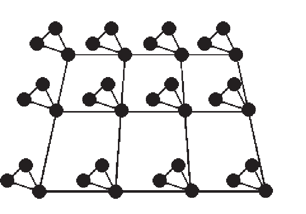
The involution on obtained by interchanging and commutes with . Hence leaves invariant the subspaces of functions which are symmetric (anti-symmetric) with respect to this involution. A non-normalized basis of simultaneous eigenfunctions for and consists of: with eigenvalue , with eigenvalue , and with eigenvalue .
Using this basis, it is easy to see that is a cyclic vector for the restriction of to . Furthermore, we can calculate :
| (4.4) |
and note that . Thus,
| (4.5) |
where are the solutions to
| (4.6) |
with and . The spectrum is purely absolutely continuous except for the presence of an infinitely degenerate eigenvalue at .
4.3. Persistence of band edge localization
The operator may include disorder, in the form of a random potential at the sites of . It is generally expected that in such a situation the spectrum of will exhibit Anderson localization (i.e., dense pure point spectrum) at all the spectral edges. (This has been rigorously shown to be true in various situations [2, 5, 6, 7, 8]). Let us note that the mechanism of gap creation via graph decorations preserves such band edge localization, even if the randomness is not introduced at all the sites of the decorated graph.
References
- [1] C. Kittel, Quantum Theory of Solids. (Wiley: New York, London, Sydney, 1963).
- [2] A. Figotin and A. Klein, “Midgap defect modes in dielectric and acoustic media,” SIAM J. Appl. Math, 58, 1748, (1998).
- [3] P. A. Deift and R. Hempel, “On the existence of eigenvalues of the Schrödinger operator in a gap of ,” Comm. Math. Phys., 103, 461, (1986).
- [4] B. Simon and T. Wolff, “Singular continuous spectrum under rank one perturbations and localization for random Hamiltonians,” Comm. Pure Appl. Math., 39, 75, (1986).
- [5] J. M.Barbaroux, J.-M. Combes, and P. D. Hislop, “Localization near band edges for random Schrödinger operators,” Helv. Phys. Acta, 70, 16, (1997).
- [6] W. Kirsch, P. Stollman, and G. Stolz, “Localization for random perturbations of periodic Schrödinger operators,” Rand. Op. Stoch. Eq., 6, 241, (1998).
- [7] F. Klopp, “Internal Lifshits tails for random perturbations of periodic Schrödinger operators.,” Duke Math. J., 98, 335, (1999).
- [8] M. Aizenman, J. H.Schenker, R. M. Friedrich, and D. Hundertmark, “Finite-volume fractional-moment criteria for Anderson localization,” to appear in Comm. Math. Phys. http://xxx.lanl.gov/abs/math-ph/9910022.