Surprises in Diffuse Scattering

For a long time, the diffuse part in diffraction spectra played only a minor role in crystallography. This was mainly due to experimental restrictions but also to a lack of theoretical studies. In this letter, we investigate some simple models with disorder, both deterministic and random, where the diffuse background of the diffraction must not be neglected in the structural analysis.

We first start with an introduction to the language of mathematical diffraction theory, which is necessary to get a full understanding of the spectrum. The following two examples have exactly the same diffraction pattern albeit their disorder is of completely different type. We then discuss models with singular continuous diffraction, a type of spectrum that is not present in classical crystallography but may appear in random structures with long range order. This is followed by the Ising lattice gas where the Bragg spectrum alone does not reflect the correct symmetry. Last, we compare square ice with an alternative model that can only be distinguished by the diffuse scattering.

Let us recall some notions of diffraction theory [5, 3], adapted to our purposes using the measure theoretic approach [8]. On the assumption of kinematical diffraction in the Fraunhofer picture, the diffracted intensity per atom $\widehat{\gamma}_{\omega}$ is given by the Fourier transform of the autocorrelation $\gamma_{\omega}$. Let the unit point measure (Dirac distribution) $\delta_{x}$ idealize an atom at position $x$ and $\Lambda$ denote the point set of all possible atomic positions. Then the atomic structure is described by the so-called weighted Dirac comb

where $w(x)\in\{0,1\}$ indicates whether the point $x$ is actually occupied or not. More generally, $w(x)$ can be a bounded complex weight function. The autocorrelation (Patterson function) $\gamma_{\omega}$, assuming it is well defined, is given by

with $\Delta=\Lambda-\Lambda$ being the set of difference vectors which we assume discrete and closed. The autocorrelation coefficient $\nu(z)$ can be calculated according to

where $B_{R}$ is the ball of radius $R$ around the origin, $\Lambda_{R}=\Lambda\cap B_{R}$ and $\overline{\hphantom{x}}$ complex conjugation. If $w(x)\in\{0,1\}$, $\nu(z)$ is the frequency of having two scatterers at distance $z$.

The Fourier transform of a function $\phi$ is

and we use the standard theory of tempered distributions from here, see [3] for our conventions.

The diffraction image, $\widehat{\gamma}_{\omega}$, is a positive measure that tells us how much intensity is scattered into a given volume element. So, by the general decomposition theorem [16, Ch. I.4], it admits a unique decomposition with respect to Lebesgue’s measure into three parts, $\widehat{\gamma}_{\omega}=(\widehat{\gamma}_{\omega})_{pp}+(\widehat{\gamma}_{\omega})_{sc}+(\widehat{\gamma}_{\omega})_{ac}$. The pure point part $(\widehat{\gamma}_{\omega})_{pp}$ consists of the Bragg peaks, the absolutely continuous $(\widehat{\gamma}_{\omega})_{ac}$ corresponds to the usual diffuse background that can often be described as a continuous function, otherwise as an $L^{1}$-function. The singular continuous component $(\widehat{\gamma}_{\omega})_{sc}$ lies somewhere in between, i.e. it is neither a smooth function nor “as singular” as a Bragg peak, for a precise definition see [16].

In the following, we present two one-dimensional examples with completely different type of (dis)order but displaying the same diffraction spectrum, i.e. they are homometric.

The first model is a Bernoulli system on $\mathbb{Z}$. The structure is given by the stochastic Dirac comb $\omega^{B}=\sum_{m\in\mathbb{Z}}\eta^{B}(m)\delta_{m}$ where $\eta^{B}(m)$ is a family of random variables that take the values $h_{1}$ and $h_{2}$ with probabilities $p_{1}$ and $p_{2}$. For such a lattice gas, one can prove [3, 4] that its diffraction measure almost surely consists of a uniform pure point and a constant absolutely continuous part,

with mean $\langle\boldsymbol{h}\rangle=p_{1}h_{1}+p_{2}h_{2}$ and variance $\text{Var}(\boldsymbol{h})=\langle|\boldsymbol{h}|^{2}\rangle-|\langle\boldsymbol{h}\rangle|^{2}$. For $h_{1}=1$, $h_{2}=0$ and $p_{1}=p_{2}=1/2$, we have $|\langle\boldsymbol{h}\rangle|^{2}=\text{Var}(\boldsymbol{h})=1/4$.

Let us compare this with the Rudin-Shapiro sequence, where the atoms are distributed deterministically. We construct $\omega^{RS}=\sum_{m\in\mathbb{Z}}\eta^{RS}(m)\delta_{m}$ according to the rule

Alternatively, this sequence may be defined via a substitution rule on a four letter alphabet [6]. For the initiate, we add that we use the square of the traditional substitution to get the fixed point of the bi-infinite sequence. The diffraction spectrum can be calculated rigorously [15, pp. 165–168]. With our choice of the scattering strenghts, this results in

Amazingly, though the structure is completely deterministic, its two-point correlations are destroyed systematically so that only a constant diffuse background remains in $\widehat{\gamma}_{\omega}$.

Therefore, with $h_{1}=1$ and $h_{2}=0$, we have $\widehat{\gamma}_{\omega}^{B}=\widehat{\gamma}_{\omega}^{RS}$, a distinction of the original structure on the basis of the diffraction spectrum is impossible. Even for finite systems, the slight difference in the fluctuations of the background is almost undetectable. Since the Fourier transform is unique, this means that the Rudin-Shapiro sequence is homometric to the above Bernoulli chain (a statement which is true with probability one). The remarkable feature of this example is the inclusion of a diffuse background, see [17] for other cases of homometry.

Note that this example explores the full entropy range: the Bernoulli case has entropy $\log 2$, the maximal value for a binary system, while Rudin-Shapiro has entropy 0. It is clear that one can find other examples with the same diffraction image but entropy between these extremal values. So, a resolution of the corresponding reconstruction problem, unless extra information is available, needs an optimization approach, e.g. by choosing the structure which maximizes the configuration entropy.

There is no simple characterization of the singular continuous part of a diffraction spectrum, since this term covers the whole range (in the sense of tempered distributions) between a continuous function, resp. $L^{1}$-function, and a Dirac distribution. As indication one may use the scaling behaviour [6, 2] of the intensities with the system size $N$: $\widehat{\gamma}_{pp}\sim N$, $\widehat{\gamma}_{ac}\sim const.$ and $\widehat{\gamma}_{sc}\sim N^{\alpha}$, $0<\alpha<1$, but this recipe is not correct in general [10]. A classical example where the scaling argument yields the right answer is the Thue-Morse sequence [15, 6]. Singular continuous spectra usually appear in structures where the constructive interference that is responsible for the Bragg peaks is impaired by some randomness. Nonetheless, some long range order is still strong enough to prevent the peaks from becoming completely diffuse. Note that singular “peaks” can never be isolated – a property that further complicates their analysis.

As an illustration in one dimension, let us consider a “tiling” of the line without gaps and overlaps which consists of two prototiles (intervals) of length 1 and $\tau=(1+\sqrt{5})/2$. The unit scatterers are located on the left endpoints of the intervals. By placing the intervals randomly with arbitrary (but fixed) probabilities, the resulting spectrum is absolutely continuous except for the trivial Bragg peak at $k=0$, see [3, Thm. 2]. On the other hand, arranging these intervals as a Fibonacci sequence leads to the well-known quasicrystal with purely discrete diffraction spectrum, cf [8].

With the same tiles, one can now also construct a “structure intermediate between quasiperiodic and random”. This is achieved using the so-called circle sequence [2]. The positions $x_{n}$ of the atoms are given by

where $0<\beta<1$, $\mathbf{1}_{[0,\beta)}$ is the characteristic function of the interval $[0,\beta)$ and $x_{0}$, $\xi\in\mathbb{R}$ are parameters; assume $x_{0}=0$ for simplicity. In order to have the same tile lengths and density $d=1/(1+\beta\xi)$ as in the Fibonacci case, we choose $\xi=\tau-1$ and $\beta=2-\tau$. As was shown by Hof [9], the circle sequence has purely singular continuous diffraction spectrum apart from the trivial Bragg peak for every irrational $\xi$, every $\beta$ and generic (“most”) $\alpha$. Nevertheless, the assessment in each explicit case is open.

In two dimensions, a straightforward generalization of the above mentioned Thue-Morse chain is given by the next example. It is constructed by using a two-dimensional substitution rule [1, 7] on a two-letter alphabet:

or, using two elementary cells with different atoms,

The resulting structure is a simple Cartesian product of Thue-Morse chains and can be treated using the method indicated in [3, Sec. 4]. The diffracted intensity is a product measure $\widehat{\gamma}_{\omega}^{2\text{D}}=\widehat{\gamma}_{\omega^{(1)}}^{\text{TM}}\cdot\widehat{\gamma}_{\omega^{(2)}}^{\text{TM}}$ of the corresponding one-dimensional intensities $\widehat{\gamma}_{\omega^{(i)}}^{\text{TM}}$ (compare [6]). We assign scattering strenghts of $+1$ (full circles) and $-1$ (open circles) to the atoms. Taking values $1$ and $0$ would just lead to an additional, trivial Bragg part on $\mathbb{Z}^{2}$. The remaining diffracted intensity is a product of singular continuous measures [15, 6] and thus itself purely singular continuous (Fig. 2). We have to emphasize that this singular continuous behaviour is by no means recognizable from the shape of the peaks and the decrease of their wings. The most likely fit is given by Gaussians, but this is also the case for true Bragg peaks.

The explicit scaling of the peaks with the system size can be obtained by applying the formulae of [6, Sec. 4.3] to our product structure.

It’s worth taking a glance at the well-known 2D Ising model where, in contrast to the previous examples, we have some interaction between the atoms. In the lattice gas formulation, we place atoms and holes (scattering strengths 1 and 0) on the square lattice subjected to coupling constants $K_{i}=J_{i}/k_{B}T>0$ in $x$- and $y$-direction. There is a phase transition at $(\sinh(2K_{1})\sinh(2K_{2}))^{-1}=1$. One can show [3] that the pure point part of the diffraction spectrum is fourfold symmetric for all $K_{i}$ and has the form

where $\rho$ is the ensemble average of the number of scatterers per unit volume, $1/2\leq\rho\leq 1$.

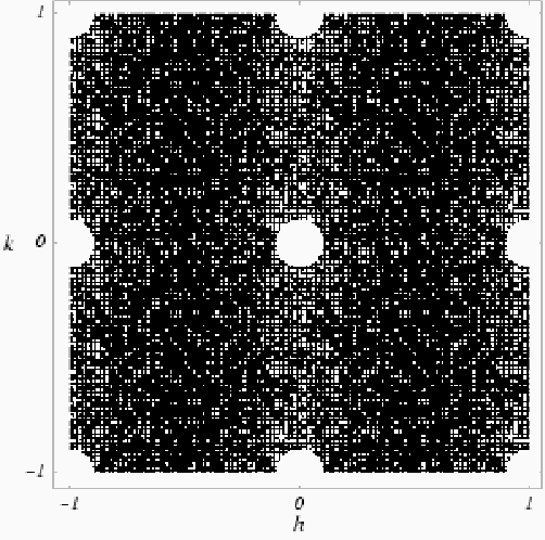
The correct (two-fold) symmetry is visible only from the diffuse part of the spectrum, the Bragg part alone is misleading. Using the asymptotic behaviour of the correlation functions, the background can be shown to be an absolutely continuous measure [3], which can be represented by a continuous function. The background concentrates around the Bragg peaks, as expected for an attractive interaction.

Square ice is another example for which the relevant structural information of the diffraction image is only contained in the diffuse background. In this model, oxygen atoms are sitting on the vertices of a square lattice, see Fig. 4. The hydrogens are placed on the edges with a distance of $1/3$ to the next O according to the following ice (or Bernal-Fowler) rules ([14] and references therein):

1. 1.

   There are two hydrogens adjacent to each oxygen.

2. 2.

   There is only one hydrogen per bond.

By using the equivalence to a special case of the six-vertex model, Lieb [12] solved the ice model and calculated its residual entropy to be $\frac{3}{2}\log\frac{4}{3}$. Although calorimetric measurements on three-dimensional ice confirmed the predicted value of the entropy very well, it was almost impossible to detect the hydrogen disorder in X-ray scattering experiments. Neutron studies are more promising, compare [11] where a highly disordered hydrogen structure was shown in deuterated cubic ice Ic.

Apart from the weak scattering power of the hydrogens, another more fundamental problem arises. Consider the case of a Bernoulli system where we ignore the first ice rule, so that the hydrogens are distributed with equal probability independently of the others.

By assigning scattering strengths $h_{\text{O}}$ and $h_{\text{H}}$ to the atoms, a straightforward calculation yields the autocorrelation of the Bernoulli model:

Thus, the Bragg part is given by $(\boldsymbol{k}=(k_{1},k_{2}))$

and the absolutely continuous background can be represented by the continuous function

But due to the same averaged occupation probabilities of the hydrogens in the ice and the Bernoulli model, their pure point parts are indistinguishable. In other words, Eq. (12) is valid for the case of square ice, too. The background is different, of course, but very weak, in particular because, in reality, $h_{\text{O}}\gg h_{\text{H}}$.

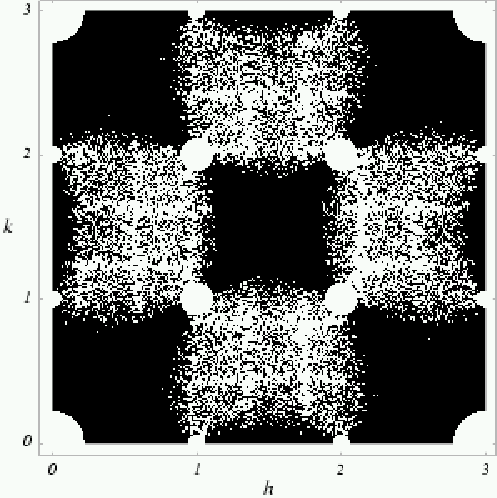
Fig. 5 displays the diffraction image of square ice. To focus on the contribution of the hydrogens, we set $h_{\text{O}}=0$. Positive $h_{\text{O}}$ would result in an increase of intensity of the Bragg peaks, except for the case of $h_{\text{O}}=h_{\text{H}}$ where we have extinction at $(k_{1},k_{2})=(1,1)$, (1,2), (2,1) and (2,2), according to Eq. (12). The continuous background, however, depends only on $h_{\text{H}}$, as in the Bernoulli case.

We have no explicit formula for the background in the ice model, since the correlation functions are not known, but we can calculate the diffraction image numerically (FFT) from a pattern of a Monte Carlo simulation, see [13, Ch. 7] for the method. The decay of the correlations suggests that the background is an absolutely continuous measure and there is no singular continuous component present. Note that the interpretation of the diffuse part is more involved here – it needs to include multi-particle effective interactions.

References

- [1] J.-P. Allouche and M. Mendès France. Automata and automatic sequences, in: “Beyond Quasicrystals”, eds. F. Axel and D. Gratias, Springer-Verlag, Berlin (1995), pp. 293–367.
- [2] S. Aubry, C. Godrèche and J. M. Luck, Scaling properties of a structure intermediate between quasiperiodic and random, J. Stat. Phys. 51 (1988), 1033–1075.
- [3] M. Baake and M. Höffe, Diffraction of random tilings: some rigorous results, J. Stat. Phys. 99 (2000), 219–261; math-ph/9904005.
- [4] M. Baake and R. V. Moody, Diffractive point sets with entropy, J. Phys. A 31 (1998), 9023–39.
- [5] J. M. Cowley, Diffraction Physics, 3rd ed., North-Holland, Amsterdam (1995).
- [6] C. Godrèche and J. M. Luck, Multifractal analysis in reciprocal space and the nature of the Fourier transform of self-similar structures, J. Phys. A 23 (1990), 3769–3797.
- [7] J. Hermisson, Aperiodische Ordnung und Magnetische Phasenübergänge, PhD-Thesis (Universität Tübingen), Shaker-Verlag, Aachen (1999).
- [8] A. Hof, On diffraction by aperiodic structures, Commun. Math. Phys. 169 (1995), 25–43.
- [9] A. Hof, On a “Structure intermediate between quasiperiodic and random”, J. Stat. Phys. 84 (1996), 309–320.
- [10] A. Hof, On scaling in relation to singular spectra, J. Stat. Phys. 184 (1997), 567–577.
- [11] W. F. Kuhs, D. V. Bliss and J. L. Finney, High-resolution neutron powder diffraction study of ice Ic, J. Phys. Coll. (Paris) 48 (1987), C1-631–636.
- [12] E. H. Lieb, Residual entropy of square ice, Phys. Rev. 162 (1967), 162–172.
- [13] M. E. J. Newman and G. T. Barkema, Monte Carlo Methods in Statistical Physics, Clarendon Press, Oxford (1999).
- [14] V. F. Petrenko and R. W. Whitworth, Physics of Ice, Oxford University Press, Oxford (1999).
- [15] M. Queffélec, Substitution Dynamical Systems – Spectral Analysis, Springer-Verlag, Berlin (1987).
- [16] M. Reed and B. Simon, Methods of Modern Mathematical Physics: I. Functional Analysis, 2nd ed., Academic Press, San Diego (1980).
- [17] E. Zobetz, One-dimensional quasilattices: Fractally shaped atomic surfaces and homometry, Acta Cryst. A 49 (1993), 667–676.