IIntroduction

DAMTP/97-3

Jan.,1997

hep-th/9702003

Graphical Classification of Global SO(n) Invariants
and
Independent General Invariants

Shoichi ICHINOSE and Noriaki IKEDA^†

DAMTP, University of Cambridge,

Silver Street, Cambridge CB3 9EW, UK[1]

^†Research Institute for Mathematical Sciences

Kyoto University, Kyoto 606-01, Japan[2]

Abstract

This paper treats some basic points in general relativity and in its perturbative analysis. Firstly a systematic classification of global SO(n) invariants, which appear in the weak-field expansion of n-dimensional gravitational theories, is presented. Through the analysis, we explain the following points: a) a graphical representation is introduced to express invariants clearly; b) every graph of invariants is specified by a set of indices; c) a number, called weight, is assigned to each invariant. It expresses the symmetry with respect to the suffix-permutation within an invariant. Interesting relations among the weights of invariants are given. Those relations show the consistency and the completeness of the present classification; d) some reduction procedures are introduced in graphs for the purpose of classifying them. Secondly the above result is applied to the proof of the independence of general invariants with the mass-dimension $M^{6}$ for the general geometry in a general space dimension. We take a graphical representation for general invariants too. Finally all relations depending on each space-dimension are systematically obtained for 2, 4 and 6 dimensions.

PACS NO: 02.70.-c, 04.20.-q, 04.60.-m, 02.40.Pc

I Introduction

In classical and quantum gravity, the most important elements are invariants under the general coordinate transformation (referred to as general invariants) because they are independent of a chosen coordinate. Physical quantities can be expressed as functions of them. The main problem we address in this paper is how to find all independent general invariants for each space-dimension. It is highly non-trivial because of the high symmetry of Riemann tensors and their products.[3, 4] As far as general invariants with lower mass-dimensions[5] are concerned, it is practically no problem because we have much experience in the past. However we encounter general invariants with higher mass-dimensions in some cases such as when we consider gravitational theories in the higher space-dimensions (ex. Weyl anomaly in a higher dimensional gravity-matter theory) or when we consider higher-order quantum corrections there (ex. Counter-terms at higher-order or higher-order effective action). As the mass-dimension of general invariants increases, the above problem becomes serious. At present, there seems to be no general way of fixing complete and independent general invariants.

With such a direction in mind, an approach to treat general invariants is given in [4], where a graphical representation is introduced. The problem of listing all general invariants is transformed to that of listing all closed graphs. It works for a general geometry in general space-dimension. Some graph relations are introduced to express some relations between Riemann tensors such as Bianchi identity and the cyclic identity. It is a powerful technique to find relations between general invariants. However, as noted in the discussion of [4], the approach does not guarantee the independence between finally listed ones. It gives only the sufficient terms as the list of complete and independent general invariants. The final list of terms could still involves linearly dependent terms. In this paper, we provide another approach to prove the independence of general invariants , as local functions, in the final list.

As far as local properties are concerned, it is sufficient to consider them in the weak-field perturbation around flat space.

\displaystyle g_{\mu\nu}=\delta_{\mu\nu}+h_{\mu\nu}{\quad,}\quad|h_{\mu\nu}|\ll 1{\quad,}

(1)

where $\mu,\nu=1,\cdots,n$ and $\delta_{\mu\nu}$ is the flat space metric. The advantages of this “weak-field”(or “linear”) representation, compared with the use of the full metric $g_{\mu\nu}$ and its inverse $g^{\mu\nu}$ , are a) there are no ’inverse’ fields and every general invariant is expressed by $h_{\mu\nu}$ and its derivatives, and b) If we express general tensors in terms of “weak-fields” representation, some non-linear relations[6] , such as the Bianchi identity and the cyclic identity, are automatically satisfied at each order of $h$ . Each general invariant is expanded as an infinite power series in $h_{\mu\nu}$ . Among many expanded terms, we focus mainly on the ’products’ of $\partial_{\mu}\partial_{\nu}h_{\alpha\beta}$ , because they turn out to give sufficient information to determine important quantities. As for general terms, we will make comments in Sec.VI and Sec.X. In [7] ( we call this ’paper (I)’ ), we introduced a graphical representation for the ’products’ of $\partial_{\mu}\partial_{\nu}h_{\alpha\beta}$ , and examined some basic definitions and lemmas, some features of the graphs. Paper (I) deals mainly with the case of $\partial\partial h$ - and $(\partial\partial h)^{2}$ -tensors. In this paper we study $(\partial\partial h)^{3}$ -tensors, where we can see a more general structure valid for general invariants with higher mass-dimensions. We classify $(\partial\partial h)^{3}$ -invariants completely. The result is applied to the proof of independence of general invariants with dimension $M^{6}$ . We prove it for a general geometry in a general space-dimension.

After listing all independent general invariants in a general dimension, we examine them in each space-dimension in order to find additional relations depending on the space-dimension. The approach of [4] is applied and 2, 4 and 6 space-dimensions are considered.

Many graphs are presented to show their usefulness. We can easily identify a tensor or an invariant with many suffixes involved. One of its important advantages is we can utilize the graph topology in explicit tensor calculation ( in computer ). We introduce some indices to represent the graph topology. The explicit calculational result of weak field expansion of general invariants, presented in App.E, shows the power of the present approach.

In Sec.II, we review paper (I) and explain the basic ingredients necessary for the present classification. Every SO(n)-invariant is represented by a graph. Classification is done in a two-fold way: one by the ’bondless diagram’, which is explained in Sec.III, and the other by ’reduced graphs’, which is explained in Sec.IV. Every graph is named respecting both classification schemes. In Sec.V, we introduce some indices in order to specify every graph by a set of topological numbers. The set of indices distinguishes each graph. Every graph has another number called the ’weight’, which shows the “degree of symmetry” with respect to suffix-contraction. Various identities between weights are presented in Sec.VI. They show the consistency and completeness of the present classification. Disconnected graphs are treated in Sec.VII. We devote ourselves to the classification of SO(n)-invariants from Sec.II to Sec.VII. In Sec.VIII we apply the results to general relativity and show the independence of general invariants. All special relations, between general invariants, which depend on space-dimension are explicitly obtained for 2, 4 and 6 dimensions in Sec.IX. The discussion and conclusion are made in Sec.X. Some appendices are provided in order to show the content of the text more concretely. App.A shows the full list of $(\partial\partial h)^{3}$ -invariants with their graphs and their graph names. App.B lists the indices and the weights of all $(\partial\partial h)^{3}$ -invariants. App.C deals with general invariants of a type $\nabla\nabla R\times R$ where a graph for $\partial_{\mu}\partial_{\nu}\partial_{\lambda}\partial_{\sigma}h_{\alpha\beta}$ is introduced. App.D deals with general invariants of another type $\nabla R\times\nabla R$ where a graph for $\partial_{\mu}\partial_{\nu}\partial_{\lambda}h_{\alpha\beta}$ is introduced. App.E lists the contribution to $(\partial\partial h)^{3}$ -terms of some general invariants with mass-dimension $M^{6}$ . App.F shows all graphs of general invariants with $M^{6}$ -dimension. Some anti-symmetrized quantities, which are used in Sec.IX, are defined graphically in App.G.

II Graphical Representation of SO(n)-Invariants

We briefly explain some basic terminology and an important lemma, introduced in paper (I), which are necessary for the present paper.

The 4-th rank global SO(n) tensor(4-tensor), $\partial_{\mu}\partial_{\nu}h_{\alpha\beta}$ is graphically represented in Fig.1.

Refer to caption — Figure 1: 4-tensor $\partial_{\mu}\partial_{\nu}h_{\alpha\beta}$

Dotted lines, a rigid line, a vertex with and without a crossing mark are called suffix-lines, a bond, a h-vertex and a dd-vertex respectively. We graphically represent suffix contraction by gluing two corresponding suffix-lines. As an example, $A1=\partial_{\sigma}\partial_{\lambda}h_{\mu\nu}\cdot\partial_{\sigma}\partial_{\nu}h_{\mu\lambda}$ is represented in Fig.2.

Generally suffix-lines in a SO(n)-invariant are closed. We call these suffix-loops. Let us state a useful lemma on a general SO(n)-invariant made of $s$ $\partial\partial h$ -tensors. It will be used in Sec.III to classify graphs in terms of the vertex (h or dd)-distribution in suffix-loops. .

Lemma

Let a general $(\partial\partial h)^{s}$ -invariant ( $s=1,2,\cdots$ ) have $\underline{l}$ suffix-loops. Let each loop have $v_{i}$ h-vertices and $w_{i}$ dd-vertices ( $i=1,2,\cdots,\underline{l}-1,\underline{l}$ ). We have the following necessary conditions for $s,\underline{l},v_{i}\ \mbox{and }w_{i}$ .

	$\displaystyle\sum_{i=1}^{\underline{l}}v_{i}=s{\quad,}\quad\sum_{i=1}^{\underline{l}}w_{i}=s{\quad,}$
	$\displaystyle v_{i}\geq 0{\quad,}\quad w_{i}\geq 0{\quad,}\quad v_{i}+w_{i}\geq 1{\quad,}$		(2)
	$\displaystyle v_{i}\ ,\ w_{i}\ =0,1,2,\cdots\quad,\quad\underline{l}=1,2,3,\cdots,2s-1,2s{\quad.}$

It is useful, for classifying graphs, to introduce a bondless diagram which is obtained by deleting all bonds within a graph. For $A1$ of Fig.2, the corresponding bondless diagram is shown in Fig.3

, where a small circle is used to represent a dd-vertex explicitly.

Generally an SO(n)-invariant is composed of some suffix-loops. For each loop, we define two indices, the bond changing number (bcn) and the vertex changing number (vcn), in the following way.

Def: bcn[ ] and vcn[ ] are defined for each suffix-loop as follows[8]. When we trace the suffix-line of a suffix-loop, starting from a vertex in a certain direction, we generally pass some vertices, and finally come back to the starting vertex. When we move, in the tracing, from one vertex to the next vertex, we compare the bonds to which the two vertices belong, and their vertex types. If the bonds are different, we set $\Delta\mbox{\lx@text@underline{bcn}}=1$ , otherwise $\Delta\mbox{\lx@text@underline{bcn}}=0$ , If the vertex-types are different, we set $\Delta\mbox{\lx@text@underline{vcn}}=1$ , otherwise $\Delta\mbox{\lx@text@underline{vcn}}=0$ . For the i-th loop, we sum the number $\Delta\mbox{\lx@text@underline{bcn}}$ and $\Delta\mbox{\lx@text@underline{vcn}}$ while tracing the loop and assign as $\sum_{\mbox{along i-loop}}\Delta\mbox{\lx@text@underline{bcn}}\equiv$ bcn[i], $\sum_{\mbox{along i-loop}}\Delta\mbox{\lx@text@underline{vcn}}\equiv$ vcn[i].

bcn[ ] and vcn[ ] will be used, in Sec.IV and Sec.III respectively, for classifying graphs.

In paper (I), we have shown, using the graphical representation, that all independent invariants are

\displaystyle P\equiv\partial_{\mu}\partial_{\mu}h_{\alpha\alpha}{\quad,}\quad Q\equiv\partial_{\alpha}\partial_{\beta}h_{{\alpha\beta}}{\quad,}\quad

(3)

for $\partial\partial h$ -invariants and

	$\displaystyle A1=\partial_{\sigma}\partial_{\lambda}h_{\mu\nu}\cdot\partial_{\sigma}\partial_{\nu}h_{\mu\lambda}\ ,\ A2=\partial_{\sigma}\partial_{\lambda}h_{\lambda\mu}\cdot\partial_{\sigma}\partial_{\nu}h_{{\mu\nu}}\ ,\ A3=\partial_{\sigma}\partial_{\lambda}h_{\lambda\mu}\cdot\partial_{\mu}\partial_{\nu}h_{\nu\sigma}\ ,$
	$\displaystyle B1=\partial_{\nu}\partial_{\lambda}h_{\sigma\sigma}\cdot\partial_{\lambda}\partial_{\mu}h_{{\mu\nu}}\ ,\ B2=\partial^{2}h_{\lambda\nu}\cdot\partial_{\lambda}\partial_{\mu}h_{{\mu\nu}}\ ,\ B3=\partial_{\mu}\partial_{\nu}h_{\lambda\sigma}\cdot\partial_{\mu}\partial_{\nu}h_{{\lambda\sigma}}\ ,$
	$\displaystyle B4=\partial_{\mu}\partial_{\nu}h_{\lambda\sigma}\cdot\partial_{\lambda}\partial_{\sigma}h_{{\mu\nu}}\ ,\ Q^{2}=(\partial_{\mu}\partial_{\nu}h_{{\mu\nu}})^{2}\ ,$
	$\displaystyle C1=\partial_{\mu}\partial_{\nu}h_{\lambda\lambda}\cdot\partial_{\mu}\partial_{\nu}h_{\sigma\sigma}\ ,\ C2=\partial^{2}h_{{\mu\nu}}\cdot\partial^{2}h_{{\mu\nu}}\ ,\ C3=\partial_{\mu}\partial_{\nu}h_{\lambda\lambda}\cdot\partial^{2}h_{{\mu\nu}}\ ,$
	$\displaystyle PQ=\partial^{2}h_{\lambda\lambda}\cdot\partial_{\mu}\partial_{\nu}h_{{\mu\nu}}\ ,\ P^{2}=(\partial^{2}h_{\lambda\lambda})^{2}\ ,$		(4)

for $(\partial\partial h)^{2}$ -invariants (totally 13 invariants). In Fig.4, an invariant $PQ$ in (4) is graphically shown.

When a diagram is composed of some parts which are not connected by suffix-lines or bonds , as in Fig.4, we say it is disconnected. Otherwise , as in Fig.2, it is referred to as connected.

III Classification of $(\partial\partial h)^{3}$ -Invariants by Bondless Diagrams

Let us first denote a suffix loop, with $v$ h-vertices, $w$ dd-vertices and a vertex changing number vcn as

\displaystyle\left(\begin{array}[]{c}v\\ w\end{array}\right)_{\mbox{\lx@text@underline{vcn}}}{\quad.}

In Fig.5, all bondless diagrams that appear in suffix-loops of $(\partial\partial h)^{3}$ -invariants, are displayed graphically with the above notation.

In this section, we classify $(\partial\partial h)^{3}$ -invariants by bondless diagrams. Taking $s=3$ in (2), we list up all cases as follows. In the following, vcn is omitted when the omission does not cause ambiguity in specifying a bondless diagram.

(i) $\underline{l}=1$

\displaystyle(1A):\left(\begin{array}[]{c}3\\ 3\end{array}\right)_{6}{\quad,}\quad(1B):\left(\begin{array}[]{c}3\\ 3\end{array}\right)_{4}{\quad,}\quad(1C):\left(\begin{array}[]{c}3\\ 3\end{array}\right)_{2}{\quad.}

(ii) $\underline{l}=2$

	$\displaystyle(2A):\left(\begin{array}[]{c}0\\ 3\end{array}\right)\left(\begin{array}[]{c}3\\ 0\end{array}\right),(2B):\left(\begin{array}[]{c}0\\ 2\end{array}\right)\left(\begin{array}[]{c}3\\ 1\end{array}\right),(2C):\left(\begin{array}[]{c}1\\ 3\end{array}\right)\left(\begin{array}[]{c}2\\ 0\end{array}\right),(2D):\left(\begin{array}[]{c}1\\ 2\end{array}\right)\left(\begin{array}[]{c}2\\ 1\end{array}\right),$
	$\displaystyle(2E_{a}):\left(\begin{array}[]{c}2\\ 2\end{array}\right)_{2}\left(\begin{array}[]{c}1\\ 1\end{array}\right),(2E_{b}):\left(\begin{array}[]{c}2\\ 2\end{array}\right)_{4}\left(\begin{array}[]{c}1\\ 1\end{array}\right),(2F_{a}):\left(\begin{array}[]{c}2\\ 3\end{array}\right)_{2}\left(\begin{array}[]{c}1\\ 0\end{array}\right),(2F_{b}):\left(\begin{array}[]{c}2\\ 3\end{array}\right)_{4}\left(\begin{array}[]{c}1\\ 0\end{array}\right),$
	$\displaystyle(2G_{a}):\left(\begin{array}[]{c}0\\ 1\end{array}\right)\left(\begin{array}[]{c}3\\ 2\end{array}\right)_{2},(2G_{b}):\left(\begin{array}[]{c}0\\ 1\end{array}\right)\left(\begin{array}[]{c}3\\ 2\end{array}\right)_{4}.$

(iii) $\underline{l}=3$

	$\displaystyle(3A):\left(\begin{array}[]{c}3\\ 1\end{array}\right)\left(\begin{array}[]{c}0\\ 1\end{array}\right)\left(\begin{array}[]{c}0\\ 1\end{array}\right),(3B):\left(\begin{array}[]{c}3\\ 0\end{array}\right)\left(\begin{array}[]{c}0\\ 2\end{array}\right)\left(\begin{array}[]{c}0\\ 1\end{array}\right),(3C):\left(\begin{array}[]{c}2\\ 0\end{array}\right)\left(\begin{array}[]{c}1\\ 0\end{array}\right)\left(\begin{array}[]{c}0\\ 3\end{array}\right),$
	$\displaystyle(3D):\left(\begin{array}[]{c}2\\ 1\end{array}\right)\left(\begin{array}[]{c}1\\ 0\end{array}\right)\left(\begin{array}[]{c}0\\ 2\end{array}\right),(3E):\left(\begin{array}[]{c}2\\ 0\end{array}\right)\left(\begin{array}[]{c}1\\ 1\end{array}\right)\left(\begin{array}[]{c}0\\ 2\end{array}\right),(3F_{a}):\left(\begin{array}[]{c}2\\ 2\end{array}\right)_{2}\left(\begin{array}[]{c}1\\ 0\end{array}\right)\left(\begin{array}[]{c}0\\ 1\end{array}\right),$
	$\displaystyle(3F_{b}):\left(\begin{array}[]{c}2\\ 2\end{array}\right)_{4}\left(\begin{array}[]{c}1\\ 0\end{array}\right)\left(\begin{array}[]{c}0\\ 1\end{array}\right),(3G):\left(\begin{array}[]{c}2\\ 0\end{array}\right)\left(\begin{array}[]{c}1\\ 2\end{array}\right)\left(\begin{array}[]{c}0\\ 1\end{array}\right),(3H):\left(\begin{array}[]{c}2\\ 1\end{array}\right)\left(\begin{array}[]{c}1\\ 1\end{array}\right)\left(\begin{array}[]{c}0\\ 1\end{array}\right),$
	$\displaystyle(3I):\left(\begin{array}[]{c}1\\ 3\end{array}\right)\left(\begin{array}[]{c}1\\ 0\end{array}\right)\left(\begin{array}[]{c}1\\ 0\end{array}\right),(3J):\left(\begin{array}[]{c}1\\ 2\end{array}\right)\left(\begin{array}[]{c}1\\ 1\end{array}\right)\left(\begin{array}[]{c}1\\ 0\end{array}\right),(3K):\left(\begin{array}[]{c}1\\ 1\end{array}\right)\left(\begin{array}[]{c}1\\ 1\end{array}\right)\left(\begin{array}[]{c}1\\ 1\end{array}\right).$

(iv) $\underline{l}=4$

	$\displaystyle(4A):\left(\begin{array}[]{c}3\\ 0\end{array}\right)\left(\begin{array}[]{c}0\\ 1\end{array}\right)\left(\begin{array}[]{c}0\\ 1\end{array}\right)\left(\begin{array}[]{c}0\\ 1\end{array}\right),(4B):\left(\begin{array}[]{c}2\\ 0\end{array}\right)\left(\begin{array}[]{c}1\\ 0\end{array}\right)\left(\begin{array}[]{c}0\\ 2\end{array}\right)\left(\begin{array}[]{c}0\\ 1\end{array}\right),$
	$\displaystyle(4C):\left(\begin{array}[]{c}2\\ 1\end{array}\right)\left(\begin{array}[]{c}1\\ 0\end{array}\right)\left(\begin{array}[]{c}0\\ 1\end{array}\right)\left(\begin{array}[]{c}0\\ 1\end{array}\right),(4D):\left(\begin{array}[]{c}2\\ 0\end{array}\right)\left(\begin{array}[]{c}1\\ 1\end{array}\right)\left(\begin{array}[]{c}0\\ 1\end{array}\right)\left(\begin{array}[]{c}0\\ 1\end{array}\right),$
	$\displaystyle(4E):\left(\begin{array}[]{c}1\\ 0\end{array}\right)\left(\begin{array}[]{c}1\\ 0\end{array}\right)\left(\begin{array}[]{c}1\\ 0\end{array}\right)\left(\begin{array}[]{c}0\\ 3\end{array}\right),(4F):\left(\begin{array}[]{c}1\\ 1\end{array}\right)\left(\begin{array}[]{c}1\\ 0\end{array}\right)\left(\begin{array}[]{c}1\\ 0\end{array}\right)\left(\begin{array}[]{c}0\\ 2\end{array}\right),$
	$\displaystyle(4G):\left(\begin{array}[]{c}1\\ 2\end{array}\right)\left(\begin{array}[]{c}1\\ 0\end{array}\right)\left(\begin{array}[]{c}1\\ 0\end{array}\right)\left(\begin{array}[]{c}0\\ 1\end{array}\right),(4H):\left(\begin{array}[]{c}1\\ 1\end{array}\right)\left(\begin{array}[]{c}1\\ 1\end{array}\right)\left(\begin{array}[]{c}1\\ 0\end{array}\right)\left(\begin{array}[]{c}0\\ 1\end{array}\right).$

(iv) $\underline{l}=5$

	$\displaystyle(5A):\left(\begin{array}[]{c}2\\ 0\end{array}\right)\left(\begin{array}[]{c}1\\ 0\end{array}\right)\left(\begin{array}[]{c}0\\ 1\end{array}\right)\left(\begin{array}[]{c}0\\ 1\end{array}\right)\left(\begin{array}[]{c}0\\ 1\end{array}\right),$
	$\displaystyle(5B):\left(\begin{array}[]{c}1\\ 0\end{array}\right)\left(\begin{array}[]{c}1\\ 0\end{array}\right)\left(\begin{array}[]{c}1\\ 0\end{array}\right)\left(\begin{array}[]{c}0\\ 2\end{array}\right)\left(\begin{array}[]{c}0\\ 1\end{array}\right),(5C):\left(\begin{array}[]{c}1\\ 1\end{array}\right)\left(\begin{array}[]{c}1\\ 0\end{array}\right)\left(\begin{array}[]{c}1\\ 0\end{array}\right)\left(\begin{array}[]{c}0\\ 1\end{array}\right)\left(\begin{array}[]{c}0\\ 1\end{array}\right).$

(iv) $\underline{l}=6$

\displaystyle(6A):\left(\begin{array}[]{c}1\\ 0\end{array}\right)\left(\begin{array}[]{c}1\\ 0\end{array}\right)\left(\begin{array}[]{c}1\\ 0\end{array}\right)\left(\begin{array}[]{c}0\\ 1\end{array}\right)\left(\begin{array}[]{c}0\\ 1\end{array}\right)\left(\begin{array}[]{c}0\\ 1\end{array}\right).

All these classification names, in addition to another classification names explained in Sec.IV, will be used when we label every $(\partial\partial h)^{3}$ -graph in App.A.

IV Classification of $(\partial\partial h)^{3}$ -Invariants by Reduced Graphs

In this section we classify all $(\partial\partial h)^{3}$ -invariants in a different way from Sec.III. We introduce two reduction procedures in graphs, which are used to classify graphs.

(i) First Reduction Procedure

The first reduction procedure is defined by identifying two vertex-types as shown in Fig.6.

This reduction makes us classify all connected $(\partial\partial h)^{3}$ -invariants (totally 19 terms) as follows: (1) $\underline{l}=1$ , Fig.7; (2) $\underline{l}=2$ , Fig.8; (3) $\underline{l}=3$ , Fig.9; (4) $\underline{l}=4$ , Fig.10. The classification naming will be explained in next item (ii).

For $\underline{l}=5$ and $6$ , there is no connected graphs.

(ii) Second Reduction Procedure

We define the second reduction procedure by reducing a bond to a vertex, as shown in Fig.11.

We get the 4 reduced graphs as shown in Fig.12.

The classification naming of (i) is due to Fig.12. We can classify all graphs of (i) as shown in Table 1.

	$\Omega$	$\Sigma$	$\Xi$	$\Theta$
$\underline{l}$ / class.	Fig.12(a)	Fig.12(b)	Fig.12(c)	Fig.12(d)
	(No of Tadpole 0)	(No of Tadpole 1)	(No of Tadpole 2)	(No of Tadpole 3)
$\underline{l}=1$	$1\Omega_{1}{\quad,}\quad 1\Omega_{2}$	$1\Sigma$	$1\Xi$	$1\Theta$
$\underline{l}=2$	$2\Omega_{1}{\quad,}\quad 2\Omega_{2}$	$2\Sigma_{1}{\quad,}\quad 2\Sigma_{2}$	$2\Xi_{1}{\quad,}\quad 2\Xi_{2}$	$2\Theta$
$\underline{l}=3$	$3\Omega$	$3\Sigma$	$3\Xi_{1}{\quad,}\quad 3\Xi_{2}$	$3\Theta$
$\underline{l}=4$			$4\Xi$	$4\Theta$

Table 1: Classification of ’vertex-type-less’ diagrams of Fig.7-10 by reducing bonds to vertices.

The complete list of all $(\partial\partial h)^{3}$ -invariants, totally 90 invariants (66 connected, 24 disconnected), are given in App.A, where graphs are classified in a two-fold way using the classification schemes of Sec.III and IV. We notice the classification labels in Sec.III refer to the distribution of dd- and h-vertices in suffix-loops, whereas those in Sec.IV refer to the topology of a graph made of bonds and suffix-loops. The completeness of the list of App.A will be shown in Sec.VI.

V Indices of $(\partial\partial h)^{3}$ -Invariants

Every graph can be characterized by its topological numbers, such as the number of suffix-loops $\underline{l}$ , which we call indices. Besides $\underline{l}$ , we have already explained bond changing number (bcn) and vertex changing number (vcn), which are another good indices. In order to specify every graph completely, we need to introduce some other indices.

The following points are advantageous when we have such a set of indices as has one-to-one correspondence with a graph (SO(n)-invariant) : 1) we can clearly read the independence of graphs( or SO(n)-invariants) because the topologically different quantities must be distinct; 2) It is indispensable in programming the calculation of quantities expressed by graphs. ( Example: weak-field expansion calculation of quantum gravity.)

V.i Tadpole Number and Type of Tadpole

Def: We call a closed suffix-loop which has only one vertex, a tadpole. The number of tadpoles a graph has, is called the tadpole number (tadpoleno) of the graph. When a tadpole has a dd(h)-vertex, its tadpole type, tadtype[ $t$ ], is defined to be 0 (1). tadtype[ $t$ ] is assigned for each tadpole : $t=1,2,\cdots$ ,tadpoleno.

For example, Fig.13 has tadpoleno=2 and tadtype[ ]=0 and 1 for each tadpole.

Generally the indices tadpoleno and tadtype[ ] are efficient for discriminating large $\underline{l}$ graphs, whereas bcn[ ] and vcn[ ] are efficient for discriminating small $\underline{l}$ graphs.

V.ii Indices for Discriminating ’Fine Structure’ of $(\partial\partial h)^{3}$ -Invariants

(i) Vertex-Type Order (Vorder)

Let us examine the graphs of Fig.14.

We cannot discriminate Graphs G9,G5 and G6 by ( $\underline{l}$ ,vcn,bcn). It is necessary to introduce a ’relative order’ of 4 vertex-types at the ends of 2 crossed bonds. Here we assign $0$ to a dd-vertex and $1$ to h-vertex as shown in Fig.14. Let us define the vertex-type order (Vorder) for each graph as the sequence of vertex-type numbers in the order, shown by an arrow in each graph of Fig.14, which is uniquely fixed by an ’isolated’ bond. For example, we have Vorder=(0,0,1,1) for Graph G9. Furthermore we take 1 st ( $\Delta V$ ), 2 nd ( $\Delta\Delta V$ ) and 3 rd ( $\Delta\Delta\Delta V$ ) difference of Vorder. For this example of G9, we have $\Delta V=(0,1,0)$ , $\Delta\Delta V=(1,-1)$ and $\Delta\Delta\Delta V=-2$ . Instead of the direct use of Vorder, $\Delta\Delta V$ and $\Delta\Delta\Delta V$ are sufficient to discriminate between the three graphs.

Another case of using Vorder is that of Fig.15.

In this case, we cannot specify the order of vertices because a ’reference’ is a vertex, not a bond. The ambiguity, however, disappears by taking the value of $|\Delta\Delta\Delta V|$ , which is used here for the discrimination. The same situation occurs for 3 more pairs: G38,G36; G32,G33; G42,G39.

(ii) Number of dd-vertices (ddverno[ ]) and of h-vertices (hverno[ ])

In order to discriminate G18 and G20 of Fig.16, we introduce the number of dd-vertices (ddverno[ $i$ ], $i=1,2,\cdots,\underline{l}$ ) and that of h-vertices (hverno[ $i$ ], $i=1,2,\cdots,\underline{l}$ ) for each loop $i$ as an index[9].

The same situation occurs in G17( $2B\Sigma_{1}$ ) and G19( $2C\Sigma_{1}$ ).

(iii) Number of crossing (crossno[ ])

Def: When a bond has its both ends ( dd-vertex and h-vertex ) in a same suffix-loop, we call it loop-bond of the suffix-loop.

Def: We consider $i$ -th suffix-loop in a graph of $(\partial\partial h)^{s}$ -invariant ( $s\geq 2$ ). Let the suffix-loop have $r$ ( $0\leq r\leq s$ ) loop-bonds. There are $r(r-1)/2$ pairs of them. For each pair, whether they are “crossed” or “not crossed” is definitely defined by tracing the vertices of both loop-bonds along the suffix-loop in a fixed direction. We define, as the total number of the crossed pairs, crossing number (crossno[ $i$ ]; $i=1,2,\cdots,\underline{l}$ ) of the $i$ -th suffix-loop.

The following are examples. Fig.13: crossno[1]=0, crossno[2]=0, crossno[3]=0; Fig.14: crossno[1]=1 for G9, G5 and G6; Fig.15: crossno[1]=1, crossno[2]=0 for G28 and G30.

G12 and G13 in Fig.17 are discriminated by crossno[ $i$ ]: crossno[1]=2 for G12, whereas crossno[1]=3 for G13.

(iv) connectivity and disconnectivity

Def: Let us consider a graph of $(\partial\partial h)^{s}$ -invariant ( $s\geq 2$ ). There are $s$ bonds and $s(s-1)/2$ different pairs of bonds. We define connectivity of the graph as the total number of those pairs which are connected by at least one suffix-line. $0\leq\mbox{\lx@text@underline{connectivity}}\leq s(s-1)/2$ .

As examples, we have the following: $A1$ (Fig.2) for connectivity=1; $PQ$ (Fig.4) for connectivity=0; $G51$ (Fig.13) for connectivity=2; $G5,G6,G9$ (Fig.14) for connectivity=3.

Def: Let us consider a graph of $(\partial\partial h)^{s}$ -invariant ( $s\geq 1$ ). Among $s$ bonds, we identify those which are connected by at least one suffix-line. Let us define, as the total number of bonds after the identification, disconnectivity+1. $0\leq\mbox{\lx@text@underline{disconnectivity}}\leq s-1$ .

As examples, we have the following: $A1$ (Fig.2) for disconnectivity=0; $PQ$ (Fig.4) for disconnectivity=1; $G23=A2Q$ (App.A) for disconnectivity=1; $G69=QQQ$ (App.A) for disconnectivity=2.

Two graphs $G71$ and $G72$ in App.A are examples which are discriminated by disconnectivity.

The list of indices for all $(\partial\partial h)^{3}$ -invariants is provided in App.B.

VI Identities between Weights

Let us define the weight of a graph in the present case. (See paper (I) for a more general case.)

Def: Let us consider a graph of $(\partial\partial h)^{s}$ -invariant ( $s\geq 1$ ). There are several ways to obtain the invariant from $s$ different 4-tensors ( $\partial_{\mu_{1}}\partial_{\nu_{1}}h_{\alpha_{1}\beta_{1}},\cdots,\partial_{\mu_{s}}\partial_{\nu_{s}}h_{\alpha_{s}\beta_{s}}$ ) by contracting $4s$ different suffixes. We define the weight of the graph as the number of all possible ways to obtain the invariant.

In App.B, all independent $(\partial\partial h)^{3}$ -invariants are listed up with weights[10] . The total sum of all weights satisfies a meaningful relation.

	$\displaystyle 10395\ (=11\times 9\times 7\times 5\times 3\times 1)=$
	$\displaystyle 384\times 9\ (G4,G5,G6,G7,G8,G9,G11,G12,G16)$
	$\displaystyle+192\times 17\ (G2,G10,G13,G15,G17,G19,G21,G22,G25,$
	$\displaystyle G29,G30,G31,G32,G37,G38,G41,G42)$
	$\displaystyle+128\times 1\ (G1)+96\times 26\ (G18,G20,G23,G24,G26,G27,G28,G33,G34,$
	$\displaystyle G35,G36,G39,G40,G44,G48,G51,G52,G55,$
	$\displaystyle G58,G59,G60,G61,G62,G64,G65,G66)+64\times 2\ (G3,G14)$		(247)
	$\displaystyle+48\times 12\ (G43,G45,G46,G47,G49,G53,G54,G56,G57,G63,G74,G81)$
	$\displaystyle+24\times 9\ (G50,G68,G71,G73,G75,G78,G80,G82,G83)+16\times 1\ (G67)$
	$\displaystyle+12\times 6\ (G72,G76,G79,G84,G85,G89)+8\times 3\ (G69,G70,G77)$
	$\displaystyle+6\times 3\ (G86,G87,G88)+1\times 1\ (G90){\quad.}$

This relation shows the completeness of the listing of App.A.

Furthermore we can see the structure of classification in relations between weights. In Sec.IV we have used two reduction procedures,Fig.6 and Fig.11. The procedure of Fig.6 reduce 66 connected graphs (see App.A) to 19 ones cited in Fig.7-10. That of Fig.11 reduces the 19 graphs to 4 ones cited in Fig.12. The following examples of relations between weights clearly show the classification structure.

(i) 66 $\rightarrow$ 19		(248)
	$\displaystyle 4^{3}\times 4\times 2\ (1\Theta)\ =512=128\ (1A\Theta)\ +384\ (1B\Theta)\ ,$
	$\displaystyle 2^{2}\times 3\times 2\times 2^{2}\ (4\Xi)\ =96$
	$\displaystyle=24\ (4B\Xi)\ +24\ (4D\Xi)+24\ (4F\Xi)+24\ (4H\Xi)\ .$	(249)
(ii) 19 $\rightarrow$ 4		(250)
	$\displaystyle(\ _{4}C_{2})^{3}\times 2^{3}\ (\Theta)\ =1728=512\ (1\Theta)\ +768\ (2\Theta)+384\ (3\Theta)+64\ (4\Theta)\ ,$
	$\displaystyle 3^{3}\times(4\times 2)\times 2^{3}\ (\Omega)\ =1728$
	$\displaystyle=768\ (1\Omega_{1})\ +256\ (1\Omega_{2})+256\ (2\Omega_{1})+384\ (2\Omega_{2})\ +64\ (3\Omega)\ .$	(251)
(iii) 66 $\rightarrow$ 4		(252)
	$\displaystyle 10395-891(\mbox{discon})=9504=1728(\Omega)+3456(\Sigma)+2592(\Xi)+1728(\Theta)\ ,$	(252)

where the total weight for the disconnected part (891) will be explained in Sec.VII.

We can simply understand the above relations in the field theory language. The initial 66 connected diagrams are produced by connected Feynman diagrams of the following lagrangian. (See a general field theory text book.)

	$\displaystyle{\cal L}={\cal L}_{0}+{\cal L}_{I}{\quad,}$
	$\displaystyle{\cal L}_{0}={\frac{1}{2}}\phi^{2}+\omega_{1}\omega_{2}{\quad,}$
	$\displaystyle{\cal L}_{I}=g_{1}\phi^{2}\omega_{1}+g_{2}\phi^{2}\omega_{2}{\quad.}$		(253)

(Of course the 24 disconnected ones (see App.A) are produced as the disconnected Feynman diagrams.) The vertices and propagators are shown in Fig.18.

The first reduction procedure (Fig.6) corresponds to taking $g_{1}=g_{2}=g/\sqrt{2},\ \omega_{1}=\omega_{2}\equiv\omega/\sqrt{2}$ in (253).

	$\displaystyle{\cal L}^{\prime}={{\cal L}_{0}}^{\prime}+{{\cal L}_{I}}^{\prime}{\quad,}$
	$\displaystyle{{\cal L}_{0}}^{\prime}={\frac{1}{2}}\phi^{2}+{\frac{1}{2}}\omega^{2}{\quad,}$
	$\displaystyle{{\cal L}_{I}}^{\prime}=g\phi^{2}\omega{\quad.}$		(254)

The vertices and propagators are shown in Fig.19.

The 19 diagrams of Fig.7-10 are produced from the above lagrangian. Integrating out the $\omega$ -integral, we obtain an effective action ${\cal L}^{\mbox{eff}}$ .

	$\displaystyle\int{\cal D}\omega\exp\{\int d^{n}x({\frac{1}{2}}\phi^{2}+{\frac{1}{2}}\omega^{2}+g\phi^{2}\omega)\}\sim\exp\{\int d^{n}x({\frac{1}{2}}\phi^{2}-{\frac{1}{2}}g^{2}\phi^{4})\}$
	$\displaystyle\equiv\exp\{\int d^{n}x{\cal L}^{\mbox{eff}}\}{\quad.}$		(255)

Fig.20 shows the vertex graphically.

This corresponds to the second reduction procedure of Fig.11. In fact the $g^{6}$ -order connected Feynman diagrams of (255) produces the diagrams of Fig.12.

This field theory approach is important when we treat general invariants with higher mass-dimensional ( $M^{8}$ , $M^{10}$ , …) cases. We comment on further generalization in Sec.X.

VII Disconnected part

Among the 90 invariants listed in App.A, there are 24 disconnected graphs. They are composed of lower dimensional invariants ( $\partial\partial h$ , $(\partial\partial h)^{2}$ ) treated in paper (I). The disconnected invariants are classified by disconnectivity. i) disconnectivity=2, 4 terms

We have the 4 terms as listed in Table 2.

	G69: QQQ	G85: PQQ	G88: PPQ	G90: PPP
weight	$2^{3}=8$	$1\times 2^{2}\times 3=12$	$1^{2}\times 2\times 3=6$	$1^{3}=1$

Table 2:

(\partial\partial h)^{3}

-terms of disconnectivity=2 and their weights

The total weight for disconnectivity=2 is 27.

ii) disconnectivity=1, 20 terms

We have the 20 terms as listed in Table 3.

	Q , 2	P , 1
A1 ,16	G24: A1Q , $16\times 2\times 3=96$	G54: A1P , $16\times 3=48$
A2 ,16	G23: A2Q , $16\times 2\times 3=96$	G53: A2P , $16\times 3=48$
A3 ,16	G26: A3Q , $16\times 2\times 3=96$	G56: A3P , $16\times 3=48$
B1 ,16	G66: B1Q , $16\times 2\times 3=96$	G81: B1P , $16\times 3=48$
B2 ,16	G61: B2Q , $16\times 2\times 3=96$	G74: B2P , $16\times 3=48$
B3 ,4	G50: B3Q , $4\times 2\times 3=24$	G72: B3P , $4\times 3=12$
B4 ,4	G68: B4Q , $4\times 2\times 3=24$	G84: B4P , $4\times 3=12$
C1 ,2	G79: C1Q , $2\times 2\times 3=12$	G87: C1P , $2\times 3=6$
C2 ,2	G76: C2Q , $2\times 2\times 3=12$	G86: C2P , $2\times 3=6$
C3 ,4	G83: C3Q , $4\times 2\times 3=24$	G89: C3P , $4\times 3=12$

Table 3:

(\partial\partial h)^{3}

-terms of disconnectivity=1. Numbers are weights. (A1

\sim

C3) are connected

(\partial\partial h)^{2}

-invariants. Q and P are

\partial\partial h

-invariants.

In Table 3, A1-C3 are $(\partial\partial h)^{2}$ -invariants and Q and P are $\partial\partial h$ -invariants ( Sec.II) . The total weight for graphs with disconnectivity=1 is 864.

Summing (i) and (ii), we see the total weight for the disconnected graphs is 891.

In sections from II to VII, we have explained the classification of $(\partial\partial h)^{3}$ -invariants only. Other types of SO(n)-invariants are classified in App.C (for $\partial^{4}h\cdot\partial^{2}h$ -invariants) and in App.D (for $\partial^{3}h\cdot\partial^{3}h$ -invariants).

VIII Independence of General Invariants

So far we have discussed the global SO(n)-invariants which appear in the weak-field perturbation of gravity. In this section we discuss properties of general invariants themselves. We consider the general space-dimension. Therefore “independence” in this section means that in the general space-dimension.

VIII.i Graphical Representation of General Tensors and Invariants

In this case also, a graphical representation is very useful[4]. We briefly explain the representation necessary for the present explanation. We can express $R_{{\mu\nu}{\lambda\sigma}},\ \nabla_{\alpha}R_{{\mu\nu}{\lambda\sigma}}\mbox{and}\ \nabla_{\alpha}\nabla_{\beta}R_{{\mu\nu}{\lambda\sigma}}$ as in Fig.21[11].

They represent their own suffix-permutation symmetries. The arrows are introduced there, and we have a simple rule: when we change the direction of arrows, we change the sign of the overall factor. This expresses the (anti-)symmetric properties: $R_{{\mu\nu}{\lambda\sigma}}=-R_{\nu\mu{\lambda\sigma}}=-R_{{\mu\nu}\sigma\lambda}=+R_{\nu\mu\sigma\lambda}$ . Relations between general invariants, like the Bianchi identity, are introduced as graphical rules. We now examine local general invariants which are made of $\nabla_{\mu},R_{{\mu\nu}{\lambda\sigma}}$ and $g_{\mu\nu}$ . As for those with lower mass dimensions, the independent ones are well known due to much experience in the past literature. For $M^{2}$ -dimension, we have

\displaystyle R{\quad,}

(256)

as a unique general invariant ( except a cosmological constant). It is graphically represented as in Fig.22. Generally suffix-lines(dotted lines) are closed for general invariants.

When a closed suffix-loop has an even number of vertices, the graph is invariant under the change of the direction of arrows. In this case we may drop the arrow in the graph ( see Fig.22) . For $M^{4}$ -dimension, we have 4 independent ones.

\displaystyle\nabla^{2}R{\quad,}\quad R^{2}{\quad,}\quad R_{\mu\nu}R^{\mu\nu}{\quad,}\quad R_{{\mu\nu}{\lambda\sigma}}R^{{\mu\nu}{\lambda\sigma}}{\quad.}

(257)

They are graphically represented as in Fig.23.

The independence of 4 terms of (257) is well known. They are those terms which appear in the Weyl anomaly in 4 dim gravity-matter theories. A proper proof of their independence, in terms of weak-expansion and its graphical representation, is given in paper (I).

VIII.ii Independent General Invariants as Local Functions

As for higher mass-dimensional cases, listing up all independent invariants is not easy. We must take into account all relations such as the Bianchi identity and the cyclic relation. The graphical representation helps greatly[4]. Using this method, we can easily list up the following 17 invariants (which were obtained, by the ordinary method, in [12, 13]) as the finally reduced $M^{6}$ -invariants[14, 15].

	$\displaystyle P_{1}=RRR{\quad,}\ \ P_{2}=RR_{\mu\nu}R^{\mu\nu}{\quad,}\ \ P_{3}=RR_{{\mu\nu}{\lambda\sigma}}R^{{\mu\nu}{\lambda\sigma}}{\quad,}$
	$\displaystyle P_{4}=R_{\mu\nu}R^{\nu\lambda}R_{\lambda}^{~\mu}{\quad,}\ \ P_{5}=-R_{{\mu\nu}{\lambda\sigma}}R^{\mu\lambda}R^{\nu\sigma}{\quad,}\ \ P_{6}=R_{{\mu\nu}{\lambda\sigma}}R_{\tau}^{~\nu{\lambda\sigma}}R^{\mu\tau}{\quad,}$
	$\displaystyle A_{1}=R_{{\mu\nu}{\lambda\sigma}}R^{\sigma\lambda}_{~~~\tau\omega}R^{\omega\tau\nu\mu}{\quad,}\ \ B_{1}=R_{{\mu\nu}\tau\sigma}R^{\nu~~~\tau}_{~\lambda\omega}R^{\lambda\mu\sigma\omega}{\quad,}$
	$\displaystyle O_{1}=\nabla^{\mu}R\cdot\nabla_{\mu}R{\quad,}\ \ O_{2}=\nabla^{\mu}R_{\lambda\sigma}\cdot\nabla_{\mu}R^{\lambda\sigma}{\quad,}$
	$\displaystyle O_{3}=\nabla^{\mu}R^{\lambda\rho\sigma\tau}\cdot\nabla_{\mu}R_{\lambda\rho\sigma\tau}{\quad,}\ \ O_{4}=\nabla^{\mu}R_{\lambda\nu}\cdot\nabla^{\nu}R^{\lambda}_{~\mu}{\quad,}$
	$\displaystyle T_{1}=\nabla^{2}R\cdot R{\quad,}\ \ T_{2}=\nabla^{2}R_{\lambda\sigma}\cdot R^{\lambda\sigma}{\quad,}\ \ T_{3}=\nabla^{2}R_{\lambda\rho\sigma\tau}\cdot R^{\lambda\rho\sigma\tau}{\quad,}\ \$
	$\displaystyle T_{4}=\nabla^{\mu}\nabla^{\nu}R\cdot R_{\mu\nu}{\quad,}\$
	$\displaystyle S=\nabla^{2}\nabla^{2}R{\quad.}$		(258)

The above 17 terms are graphically given in App.F. The above listing, however, does not guarantee that all terms of (258) are independent each other. We do not have a proper basis in the ’full metric’ treatment, which makes it difficult to show the independence. As an application of the results about the classification of SO(n)-invariants (Sec.II-VII), we can prove the independence of the above 17 terms of (258) for a general geometry in a general space-dimension. In order to show the independence as a local function, we can safely use the weak field expansion: $g_{\mu\nu}=\delta_{\mu\nu}+h_{\mu\nu}\ ,\ |h_{\mu\nu}|\ll 1$ .

(i) $S=\nabla^{2}\nabla^{2}R$ The leading order is given by $\partial^{6}h\sim O(h)$ .

\displaystyle S=\partial^{2}\partial^{2}(\partial^{2}h-\partial_{\mu}\partial_{\nu}h_{\mu\nu})+O(h^{2}){\quad.}

(259)

Other terms do not have $O(h)$ contribution, therefore $S$ is independent from others. (ii) $T_{1}\sim T_{4}$ The leading order of every term is $\partial^{4}h\times\partial^{2}h\sim O(h^{2})$ . The classification of $\partial^{4}h\cdot\partial^{2}h$ -invariants are given in App.C. The expansions of $T_{1}\sim T_{4}$ , in terms of $\partial^{4}h\cdot\partial^{2}h$ -invariants are also given there. The explicit forms of their expansions show that the 4 terms are independent. Because other terms, except $S$ , do not contribute to terms of this type, we see they can be taken as independent terms. (iii) $O_{1}\sim O_{4}$ The leading order of every term is given by $\partial^{3}h\times\partial^{3}h\sim O(h^{2})$ . In App.D, the classification of $\partial^{3}h\cdot\partial^{3}h$ -invariants are given. The expansions of $O_{1}\sim O_{4}$ , in terms of them, are also obtained explicitly. Their explicit forms show the 4 terms are independent. In the similar way to (ii), we see they can be taken as independent terms. (iv) $P_{1}\sim P_{6},A_{1},B_{1}$ The leading order of every term is given by $(\partial\partial h)^{3}\sim O(h^{3})$ . $(\partial\partial h)^{3}$ -invariants are completely classified in the text, and the results (especially the set of indices) allow us to easily calculate (by computer) the weak-field expansion. This shows the power of the present classification. The result is given in App.E, which shows the 8 terms $\{P_{1}\sim P_{6},A_{1},B_{1}\}$ are independent each other. Furthermore they are “orthogonal” in the space of 90 terms except the G3 and G13 “directions”.( $A_{1}$ and $B_{1}$ have common components to G3 and G13 “directions”. If some inner product can be defined in this “vector” space, orthogonal ones could be chosen by taking some linear combinations of $A_{1}$ and $B_{1}$ . )

From (i) $\sim$ (iv), we may say the 17 terms of (258) are independent each other as local functions, so far as symmetries valid for general space dimension are concerned.

IX Relations Valid for Only Each Dimension

It is known that, for each fixed space-dimension, there generally appear additional relations among general invariants and topological quantities (say, [16, 3, 17, 4]). This kind of relations have been noticed rather fragmentally in specific situations so far. Here we explicitly derive them in a systematic way. We still keep a general space-dimension $n$ for a while.

Let us introduce the quantity, $I^{an2}_{R}$ , graphically defined in Fig.24, where a convenient notation is introduced and is used in the following. In the figure, anti[ $\alpha,\beta$ ] means anti-symmetrization w.r.t. $\alpha$ and $\beta$ .

We define similar quantities in Fig.25 where anti[ $\alpha,\beta,\gamma$ ] and anti[ $\alpha,\beta,\gamma,\delta$ ] mean total anti-symmetrization w.r.t. ( $\alpha,\beta,\gamma$ ) and ( $\alpha,\beta,\gamma,\delta$ ) respectively. We can easily compute them by the use of algebraic calculation, and we obtain as follows.

	$\displaystyle I^{an2}_{R}=2R{\quad,}$
	$\displaystyle I^{an3}_{R^{2}}=2(-2R_{\mu\nu}R^{\mu\nu}+R^{2}){\quad,}$
	$\displaystyle I^{an4}_{R^{2}}=4(R^{2}-4R_{\mu\nu}R^{\mu\nu}+R_{{\mu\nu}{\alpha\beta}}R^{{\mu\nu}{\alpha\beta}}){\quad,}$		(260)

When we anti-symmetrize some suffixes in a given graph (general invariant) $G$ , we notice the following general facts.

1.

We generally obtain different anti-symmetrized quantities by taking different choices of the starting graph $G$ and of the number of anti-symmetrized suffixes ( $\equiv N_{an}$ ).
2.

$N_{an}$ is maximized at the number of internal dotted lines ( $\equiv N_{I}$ ): $N_{an}\leq N_{I}$ . (Ex. In Fig.25, $N_{an}=3,N_{I}=4$ for $I^{an3}_{R^{2}}$ ; $N_{an}=4,N_{I}=4$ for $I^{an4}_{R^{2}}$ .) When $N_{an}<N_{I}$ , there generally appear some choices of suffixes to be anti-symmetrized.
3.
There are two cases when we calculate anti-symmetrized quantities.
1. (a)
  
  It identically vanishes. In this case we do not have relations among invariants.
2. (b)
  
  It gives a sum of some invariants listed in Sec.VIII.

For $M^{2}$ - and $M^{4}$ - invariants, all possible non-zero anti-symmetrized quantities are given by (260).

We can do the same thing for $M^{6}$ -invariants. Anti-symmetrized quantities are defined in App.G. They are all linearly-independent non-zero ones ( except a relation in (263), which is written for an interest ) and are computed as follows. From Fig.49 of App.G, we have

	$\displaystyle I^{an3}_{P_{1}}=P_{1}-3P_{2}+2P_{4}{\quad,}$
	$\displaystyle I^{an3}_{A_{1}}=P_{4}-3P_{6}+\frac{5}{4}A_{1}-B_{1}{\quad,}$
	$\displaystyle I^{an3}_{P_{3}}=-P_{2}+P_{3}+2P_{5}-2P_{6}{\quad,}$
	$\displaystyle I^{an3}_{B_{1}(a)}=4B_{1}{\quad,}$
	$\displaystyle I^{an3}_{B_{1}(b)}=-{\frac{1}{2}}A_{1}+2B_{1}+P_{6}{\quad,}$
	$\displaystyle I^{an3}_{P_{5}}=P_{5}-{\frac{1}{2}}P_{6}{\quad,}$		(261)

The expression of $I^{an3}_{B_{1}(a)}$ implies $B_{1}$ is “self-dual”. From the Fig.50 of App.G, we have

	$\displaystyle I^{an4}_{P_{1}}=2P_{1}-10P_{2}+8P_{4}+4P_{5}{\quad,}$
	$\displaystyle I^{an4}_{A_{1}}=4P_{4}+4P_{5}-10P_{6}+3A_{1}-4B_{1}{\quad,}$
	$\displaystyle I^{an4}_{P_{3}}=-2P_{2}+2P_{3}+8P_{5}-8P_{6}+A_{1}-4B_{1}{\quad,}$
	$\displaystyle I^{an4}_{P_{6}}=-2P_{5}+2P_{6}-{\frac{1}{2}}A_{1}+2B_{1}{\quad,}$
			(262)

From the Fig.51 of App.G, we have

	$\displaystyle I^{an5}_{P_{1}}=4(P_{1}-8P_{2}+P_{3}+8P_{4}+8P_{5}-4P_{6})=2(I^{an6}_{P_{1}}-4I^{an5}_{A_{1}}){\quad,}$
	$\displaystyle I^{an5}_{A_{1}}=4(-2P_{2}+P_{3}+4P_{4}+8P_{5}-10P_{6}+2A_{1}-4B_{1}){\quad,}$
	$\displaystyle I^{an6}_{P_{1}}=4(2P_{1}-24P_{2}+6P_{3}+32P_{4}+48P_{5}-48P_{6}+8A_{1}-16B_{1}){\quad,}$		(263)

Eqs.(261)-(263) show $RRR$ -type invariants are closed within themselves for the anti-symmetrization. From the Fig.52 of App.G, we have

	$\displaystyle I^{an3}_{T_{1}(a)}=2(T_{1}-2T_{2}){\quad,}$
	$\displaystyle I^{an3}_{T_{1}(b)}=-P_{4}+P_{5}+{\frac{1}{2}}T_{1}-T_{2}{\quad,}$
	$\displaystyle I^{an3}_{T_{1}(c)}=2(T_{1}-2T_{4}){\quad,}$
	$\displaystyle I^{an3}_{T_{3}}=-P_{6}+{\frac{1}{2}}A_{1}+2B_{1}{\quad,}$
	$\displaystyle I^{an4}_{T_{1}(a)}=4(T_{1}-4T_{2}+T_{3}){\quad,}$
	$\displaystyle I^{an4}_{T_{1}(b)}=-4P_{4}+4P_{5}+2P_{6}-A_{1}-4B_{1}+T_{1}-4T_{2}+T_{3}{\quad,}$		(264)

These relations show $\nabla\nabla R\times R$ type invariants are not closed within themselves. In particular, $I^{an3}_{T_{3}}$ does not have $T_{3}$ . From the Fig.53 of App.G, we have

	$\displaystyle I^{an3}_{O_{1}(a)}=2(O_{1}-2O_{2}){\quad,}$
	$\displaystyle I^{an3}_{O_{1}(b)}=\frac{1}{4}O_{1}-O_{2}+O_{4}{\quad,}$
	$\displaystyle I^{an4}_{O_{1}}=4(O_{1}-4O_{2}+O_{3}){\quad,}$		(265)

$\nabla R\times\nabla R$ type invariants are closed within themselves.

Let us examine relations for each space-dimension.

(i) n=2

For the $n=2$ space dimension, $I^{an2}_{R}$ gives the Gauss-Bonnet relation,

\displaystyle\int d^{2}x\sqrt{g}I^{an2}_{R}=\mbox{topological invariant}{\quad.}

(266)

The invariant $R$ , (256), remains as the unique general $M^{2}$ -invariant although $\sqrt{g}R$ is a surface term (total derivative). $I^{an~i}_{*}=0\ (i\geq 3)$ give us relations. From $I^{an3}_{R^{2}}=0$ and $I^{an4}_{R^{2}}=0$ , we have the following ones between $M^{4}$ -invariants.

\displaystyle R_{{\mu\nu}{\lambda\sigma}}R^{{\mu\nu}^{\lambda\sigma}}=2R_{\mu\nu}R^{\mu\nu}=R^{2}{\quad.}

(267)

Therefore we can take, as all independent $M^{4}$ -invariants in 2 space dimension,

\displaystyle\nabla^{2}R{\quad,}\quad R^{2}{\quad.}

(268)

Relations (267) deduce the following ones between $M^{6}$ -invariants.

\displaystyle P_{1}=2P_{2}=P_{3}{\quad.}

(269)

From the vanishing of all quantities of (261)-(263), we have

\displaystyle P_{1}=4P_{4}=4P_{5}=2P_{6}=A_{1}{\quad,}\quad B_{1}=0{\quad.}

(270)

From the vanishing of all quantities of (264), we have

\displaystyle T_{1}=2T_{2}=2T_{4}=T_{3}{\quad.}

(271)

From the vanishing of all quantities of (265), we have

\displaystyle O_{1}=2O_{2}=O_{3}=4O_{4}{\quad.}

(272)

Therefore we have the following 4 terms as independent $M^{6}$ -invariants.

\displaystyle P_{1}=RRR{\quad,}\ \ O_{1}=\nabla^{\mu}R\cdot\nabla_{\mu}R{\quad,}\ \ T_{1}=\nabla^{2}R\cdot R{\quad,}\ \ S=\nabla^{2}\nabla^{2}R{\quad.}

(273)

We should note here that the above relations are derived without the use of the well-known relation between Riemann tensors which is valid only in 2 space-dimension.

\displaystyle R_{{\mu\nu}{\lambda\sigma}}={\frac{1}{2}}(g_{\mu\sigma}g_{\nu\lambda}-g_{\mu\lambda}g_{\nu\sigma})R{\quad.}

(274)

(Of course, the obtained relations are consistent with the above relation. This is a strong check of the present approach.) Because the degree of local freedom of the Riemann tensor in n-dim space is $f(n)=n^{2}(n^{2}-1)/12,n\geq 4$ , we do not have such simple relations as (274) in higher space dimension. Hence the present approach is indispensable to obtain all relations in higher space-dimension.

(ii) n=4

In the $n=4$ space dimension, $I^{an4}_{RR}$ gives the Gauss-Bonnet relation,

\displaystyle\int d^{4}x\sqrt{g}I^{an4}_{RR}=\mbox{topological invariant}{\quad.}

(275)

The four invariants (257) remain as independent general $M^{4}$ -invariants. From the vanishing of all quantities of (263), we have two independent relations between $M^{6}$ -invariants.

\displaystyle I^{an5}_{P_{1}}=0{\quad,}\quad I^{an5}_{A_{1}}=0{\quad.}

(276)

There exist no relations between $T_{i}$ ’s and $O_{i}$ ’s. Therefore we have 17-2=15 terms as independent $M^{6}$ -invariants, say,

	$\displaystyle P_{1}{\quad,}\quad P_{2}{\quad,}\quad P_{3}{\quad,}\quad P_{4}{\quad,}\quad P_{5}{\quad,}\quad A_{1}{\quad,}$
	$\displaystyle T_{1}{\quad,}\quad T_{2}{\quad,}\quad T_{3}{\quad,}\quad T_{4}{\quad,}\quad O_{1}{\quad,}\quad O_{2}{\quad,}\quad O_{3}{\quad,}\quad O_{4}{\quad,}\quad S{\quad.}$		(277)

They are considered to appear in the higher-order of the Weyl anomaly due to the graviton-loop effect if they can be properly defined. (In the usual(1-loop) Weyl anomaly, 4 terms of (257) appear).

(iii) n=6

In the $n=6$ space-dimension, $I^{an6}_{P_{1}}$ gives the Gauss-Bonnet relation,

\displaystyle\int d^{6}x\sqrt{g}I^{an6}_{P_{1}}=\mbox{topological invariant}{\quad.}

(278)

The 17 invariants (258) remain as independent general invariants.

Therefore we have confirmed that, in n space-dimension, all independent $M^{n}$ -invariants ( the (1-loop) Weyl anomaly is given by them ) are given in Sec.VIII : (256) for n=2, (257) for n=4 and (258) for n=6. Only for general invariants with higher mass-dimension $M^{m},m>n$ , the number of independent ones reduces from those given in Sec.VIII due to relations valid only for each dimension.

As a comparison, it is interesting to examine the situation in independent general invariants as counterterms. Generally the counterterms $\Delta{\cal L}$ are defined in a space integral in such a way that the action

\displaystyle\int\sqrt{g}~\Delta{\cal L}~d^{n}x{\quad,}

(279)

cancels (ultra-violet) divergences due to the quantum fluctuation. $\Delta{\cal L}$ is a sum of general invariants with ’divergent’-constant coefficients. Here we have interest in what terms could appear as independent ones. We may neglect total derivative terms because the fields are usually assumed to damp sufficiently rapidly at the boundary. As a choice, we give a complete list of independent counterterms in the following.

(i) n=2

$M^{2}$ -invariants(1-loop): no terms
$M^{4}$ -invariants(2-loop): $R^{2}$
$M^{6}$ -invariants(3-loop): $P_{1}=RRR,O_{1}=\nabla^{\mu}R\cdot\nabla_{\mu}R$

(ii) n=4

$M^{4}$ -invariants(1-loop): $R^{2},R_{\mu\nu}R^{\mu\nu}$
$M^{6}$ -invariants(2-loop): $P_{1},P_{2},P_{3},P_{4},P_{5},A_{1},O_{1},O_{2},O_{3},O_{4}$

(iii) n=6

$M^{6}$ -invariants(1-loop): $P_{1},P_{2},P_{3},P_{4},P_{5},P_{6},A_{1},O_{1},O_{2},O_{3},O_{4}$

If we consider pure gravity and impose the S-matrix condition (on-shell condition, Ricci flat condition) $R_{\mu\nu}=0$ on the above results, we see 2 dim pure gravity is finite, 4 dim case is not finite at higher-loops from 2-loop, 6 dim case is not finite at higher-loops from 1-loop. In the latter two cases, non-finite term appears as $A_{1}$ term. This is well known from the divergence problem in the S-matrix in perturbative quantum gravity[18, 19].

X Discussions and Conclusions

We have presented a way to classify SO(n)-invariants which generally appear in weak-field perturbations of (quantum) gravity. Taking the explicit example of $(\partial\partial h)^{3}$ -invariants, we have presented the general way of classification. The following important items have been explained : 1) the graphical representation of global SO(n)-tensors and invariants, 2) the weight of a graph, 3) indices characterizing a graph, 4) reduction procedures of graphs, and 5) bondless diagrams. In the higher dimensional cases, such as $(\partial\partial h)^{4}$ and $(\partial\partial h)^{5}$ ( which appear, for example, in the Weyl anomaly in 8 dim and 10 dim gravity, respectively) the same procedure can be applied except some additional indices might be required.

We have mainly discussed $(\partial\partial h)^{3}$ -invariants in the text, $\partial^{4}h\cdot\partial^{2}h$ -invariants in App.C and $(\partial^{3}h)^{3}$ -invariants in App.D. $\partial\partial h$ - and $(\partial\partial h)^{2}$ -invariants have been treated in paper (I). Clearly it must be generalized to treat all SO(n)-invariants which appear in the weak expansion of all general invariants. For such direction, we comment on the generalization of the field theory approach proposed in Sec.VI. Let us consider the following Lagrangian in $2$ space-dimension[20].

	$\displaystyle{\cal L}[\phi,\omega_{1},\omega_{2}]={\cal L}_{0}+{\cal L}_{I}{\quad,}$
	$\displaystyle{\cal L}_{0}={\frac{1}{2}}\phi^{2}+\omega_{1}\omega_{2}{\quad,}$
	$\displaystyle{\cal L}_{I}[\phi,\omega_{1},\omega_{2}]=\sum_{i=1}^{\infty}g_{i}\phi^{i}\omega_{1}+\lambda\phi^{2}\omega_{2}{\quad.}$		(280)

We assign mass-dimension as follows.

\displaystyle[{\cal L}]=M^{2}{\quad,}\quad[\phi]=M{\quad,}\quad[\omega_{1}]=M^{2}{\quad,}\quad[\omega_{2}]=M^{0}{\quad.}

(281)

Then we obtain

\displaystyle[g_{i}]=M^{-i}{\quad,}\quad[\lambda]=M^{0}{\quad.}

(282)

This result turns out to give the mass-dimension of each expanded term in the following. The generating functional of all graphs ( SO(n)-invariants, SO(n)-tensors ) is given by

	$\displaystyle W[J,K_{1},K_{2}]=\exp^{\Gamma[J,K_{1},K_{2}]}$
	$\displaystyle=\int{\cal D}\phi{\cal D}\omega_{1}{\cal D}\omega_{2}\exp\left[\int d^{2}x({\cal L}[\phi,\omega_{1},\omega_{2}]+J\phi+K_{1}\omega_{1}+K_{2}\omega_{2})\right]$
	$\displaystyle=\sum_{r=0}^{\infty}\frac{1}{r!}\left[\int d^{2}x{\cal L}_{I}(\frac{\delta}{\delta J(x)},\frac{\delta}{\delta K_{1}(x)},\frac{\delta}{\delta K_{2}(x)})\right]^{r}\exp\int d^{2}x(-{\frac{1}{2}}J(x)J(x)-K_{1}(x)K_{2}(x)){\quad.}$		(283)

All graphs of connected n-tensors appear in the n-point Green function.

\displaystyle\frac{1}{n!}\left.\frac{\delta}{\delta J(x_{1})}\frac{\delta}{\delta J(x_{2})}\cdots\frac{\delta}{\delta J(x_{n})}\Gamma[J,K_{1},K_{2}]\right|_{J=0,K_{1}=0,K_{2}=0}{\quad.}

(284)

In particular all SO(n)-invariants appear in

\displaystyle\left.\Gamma[J,K_{1},K_{2}]\right|_{J=0,K_{1}=0,K_{2}=0}{\quad.}

(285)

These quantities are given by perturbation with respect to the couplings ( $g_{1},g_{2},\cdots;\lambda$ ) in ${\cal L}_{I}$ . For example, $(\partial\partial h)^{s}$ -invariants ( $s=1,2,\cdots$ ) are given by $(g_{2}\lambda)^{s}$ -terms ( $r=2s$ ) in (285). $\partial^{4}h\cdot\partial^{2}h$ -invariants (App.C) and $\partial^{3}h\cdot\partial^{3}h$ -invariants (App.D) are given by $g_{4}\cdot g_{2}\cdot\lambda^{2}$ -terms ( $r=4$ ) and $g_{3}\cdot g_{3}\cdot\lambda^{2}$ -terms ( $r=4$ ) respectively. From the coupling-dependence, the mass-dimension of each graph is given. For example $[(g_{2}\lambda)^{s}]=M^{-2s}$ , $[g_{4}\cdot g_{2}\cdot\lambda^{2}]=M^{-6}$ and $[g_{3}\cdot g_{3}\cdot\lambda^{2}]=M^{-6}$ . They are the inverse of their mass-dimensions. The coefficient in front of each expanded term are related with the weight of the corresponding graph. The generalization using this field theory approach is useful for classification of general SO(n)-invariants.

The result is not only interesting as the mathematical (graphical) structure by itself, but also provides a very efficient computer-algorithm for the tensor calculation. As an example of a computer calculation, we have presented some results of weak-perturbation of general $M^{6}$ -invariants in App.E. They are used to prove the independence of general $M^{6}$ -invariants in Sec.VIII. Further important applications of the present result are the anomaly and the (1-loop) counterterm calculation in 6 dim quantum gravity. Generally in n-dim gravity, the Weyl anomaly is given by some combination of general invariants with dimension $M^{n}$ , and $L$ -loop counterterms are given by some combination of invariants with dimension $M^{n+2L-2}$ . In both cases, all coefficients can be fixed by the weak-field perturbation[21].

So far, we have been annoyed by the complicated tensor calculation in the analysis of (quantum) gravity. It is serious especially in a higher-dimensional case or in a higher-order case. This is because we have not known an efficient way to manipulate tensors. It is not an exaggeration to say that the complication has been a hinderence to understanding the theory of gravity. We believe the present approach provides a new possibility in analysing (quantum) gravity in such cases.

The results of Sec.IX, App.B, App.E and some others are obtained by computer calculation (FORM, C-language program).

Acknowledgement

The authors thank Prof. K.Murota (RIMS,Kyoto Univ.,Japan) for an important suggestion in Sec.IV. They express gratitude to Prof. H.Osborn for reading the manuscript and some comments. The check of the manuscript by Dr. H.Shanahan and the kind help in the computer manipulation by Dr. C.Houghton are greatly appreciated. A part of this work has been done when one of the authors (S.I.) are staying at DAMTP, Univ. of Cambridge. He thanks all members of DAMTP for hospitality. One of the authors (S.I.) thanks Japanese ministry of education for the partial financial support (Researcher No: 40193445, Institution No: 23803).

Appendix A. Full List of $(\partial\partial h)^{3}$ -Invariants

In this appendix we list up graphs of all independent $(\partial\partial h)^{3}$ -invariants. Every graph is named according to the classification scheme explained in Sec.III and IV. They are grouped with respect to the number of suffix-loops $\underline{l}$ as follows. (“con” means “connected graphs” and “discon” means “disconnected graphs”.)

(i) $\underline{l}=1$ ( 13(con)+0(discon)=13 terms ), Fig.26. (ii) $\underline{l}=2$ ( 26(con)+3(discon)=29 terms ), Fig.27 and Fig.28. (iii) $\underline{l}=3$ ( 19(con)+8(discon)=27 terms ), Fig.29 and Fig.30. (iv) $\underline{l}=4$ ( 8(con)+8(discon)=16 terms ), Fig.31 and Fig.32. (v) $\underline{l}=5$ ( 0(con)+4(discon)=4 terms ), Fig.33. (vi) $\underline{l}=6$ ( 0(con)+1(discon)=1 term ), Fig.34.

Appendix B. List of Indices of All $(\partial\partial h)^{3}$ -Invariants

Every graph can be specified completely by a set of indices which expresses its topology( see Sec.II and V). Lists of indices ( $\underline{l}$ ,tadpoleno,tadtype,bcn,vcn) and weight are given in Table 4 for G1-G13, in Table 5 for G14-G42, in Table 6 for G43-G69 and in Table 7 for G70-90. This result is coded into the program, which enables the present computer calculation. In the tables, there is a column of ’fine splitting’. These boxes show how to discriminate topologically quite similar graphs which are those graphs with the same #-number. It is explained in Subsec.V.ii of the text.

Graph No:Graph	$\underline{l}$	tadpo	tadtype	(bcn,vcn)	‘fine
Name,weight		leno			splitting’
$G1:1A\Theta,\ 128$	$1$	$0$	n	$(3,6)$
$G2:1A\Xi,\ 192$	$1$	$0$	n	$(4,6)$
$G3:1A\Omega_{2},\ 64$	$1$	$0$	n	$(6,6)$
$G4:1B\Theta,\ 384$	$1$	$0$	n	$(3,4)$
$G5:1B\Sigma-a,\ 384$	$1$	$0$	n	$(5,4)$	#1 Vorder
$G6:1B\Sigma-b,\ 384$	$1$	$0$	n	$(5,4)$	#1 Vorder
$G7:1B\Omega_{1},\ 384$	$1$	$0$	n	$(6,4)$
$G8:1B\Xi,\ 384$	$1$	$0$	n	$(4,4)$
$G9:1B\Sigma-c,\ 384$	$1$	$0$	n	$(5,4)$	#1 Vorder
$G10:1C\Xi,\ 192$	$1$	$0$	n	$(4,2)$
$G11:1C\Sigma,\ 384$	$1$	$0$	n	$(5,2)$
$G12:1C\Omega_{1},\ 384$	$1$	$0$	n	$(6,2)$	#2 crossno
$G13:1C\Omega_{2},\ 192$	$1$	$0$	n	$(6,2)$	#2 crossno

Table 4: Index list of SO(n)-Invariants

(\partial\partial h)^{3}

. G1-G13(

\underline{l}

=1)

Graph No:Graph	$\underline{l}$	tadpo	tadtype	(bcn,vcn)	‘fine
Name,weight		leno			splitting’
$G14:2A\Omega_{1},\ 64$	$2$	$0$	n	$(3,0),(3,0)$
$G15:2D\Omega_{1},\ 192$	$2$	$0$	n	$(3,2),(3,2)$
$G16:2D\Xi_{1},\ 384$	$2$	$0$	n	$(2,2),(2,2)$
$G17:2B\Sigma_{1},\ 192$	$2$	$0$	n	$(2,0),(3,2)$	#3 dd(h)verno
$G18:2B\Omega_{2},\ 96$	$2$	$0$	n	$(2,0),(4,2)$	#4 dd(h)verno
$G19:2C\Sigma_{1},\ 192$	$2$	$0$	n	$(2,0),(3,2)$	#3 dd(h)verno
$G20:2C\Omega_{2},\ 96$	$2$	$0$	n	$(2,0),(4,2)$	#4 dd(h)verno
$G21:2E_{a}\Sigma_{1},\ 192$	$2$	$0$	n	$(2,2),(3,2)$
$G22:2E_{a}\Omega_{2},\ 192$	$2$	$0$	n	$(2,2),(4,2)$
$G23:A2Q,\ 96$	$2$	$0$	n	$(0,2),(2,2)$
$G24:A1Q,\ 96$	$2$	$0$	n	$(0,2),(4,2)$
$G25:2E_{b}\Sigma_{1},\ 192$	$2$	$0$	n	$(2,2),(3,4)$
$G26:A3Q,\ 96$	$2$	$0$	n	$(0,2),(2,4)$
$G27:2F_{a}\Theta,\ 96$	$2$	$1$	$1$	$(3,2)$
$G28:2F_{a}\Sigma_{2}-a,\ 96$	$2$	$1$	$1$	$(5,2)$	#5 Vorder
$G29:2F_{a}\Xi_{2},\ 192$	$2$	$1$	$1$	$(4,2)$
$G30:2F_{a}\Sigma_{2}-b,\ 192$	$2$	$1$	$1$	$(5,2)$	#5 Vorder
$G31:2F_{b}\Xi_{2},\ 192$	$2$	$1$	$1$	$(4,4)$
$G32:2F_{b}\Theta-a,\ 192$	$2$	$1$	$1$	$(3,4)$	#6 Vorder
$G33:2F_{b}\Theta-b,\ 96$	$2$	$1$	$1$	$(3,4)$	#6 Vorder
$G34:2F_{b}\Sigma_{2},\ 96$	$2$	$1$	$1$	$(5,4)$
$G35:2G_{a}\Theta,\ 96$	$2$	$1$	$0$	$(3,2)$
$G36:2G_{a}\Sigma_{2}-a,\ 96$	$2$	$1$	$0$	$(5,2)$	#7 Vorder
$G37:2G_{a}\Xi_{2},\ 192$	$2$	$1$	$0$	$(4,2)$
$G38:2G_{a}\Sigma_{2}-b,\ 192$	$2$	$1$	$0$	$(5,2)$	#7 Vorder
$G39:2G_{b}\Theta-a,\ 96$	$2$	$1$	$0$	$(3,4)$	#8 Vorder
$G40:2G_{b}\Sigma_{2},\ 96$	$2$	$1$	$0$	$(5,4)$
$G41:2G_{b}\Xi_{2},\ 192$	$2$	$1$	$0$	$(4,4)$
$G42:2G_{b}\Theta-b,\ 192$	$2$	$1$	$0$	$(3,4)$	#8 Vorder

Table 5: Index list of SO(n)-Invariants

(\partial\partial h)^{3}

. G14-G42(

\underline{l}

=2)

Graph No:Graph	$\underline{l}$	tadpo	tadtype	(bcn,vcn)	‘fine
Name,weight		leno			splitting’
$G43:3A\Xi_{1},\ 48$	$3$	$2$	$0,0$	$(4,2)$
$G44:3A\Theta,\ 96$	$3$	$2$	$0,0$	$(3,2)$
$G45:3B\Sigma,\ 48$	$3$	$1$	$0$	$(2,0),(3,0)$
$G46:3C\Sigma,\ 48$	$3$	$1$	$1$	$(2,0),(3,0)$
$G47:3D\Sigma,\ 48$	$3$	$1$	$1$	$(2,0),(3,2)$
$G48:3D\Xi_{2},\ 96$	$3$	$1$	$1$	$(2,0),(2,2)$
$G49:3E\Omega,\ 48$	$3$	$0$	n	$(2,0),(2,0),(2,2)$
$G50:B3Q,\ 24$	$3$	$0$	n	$(0,2),(2,0),(2,0)$
$G51:3F_{a}\Theta,\ 96$	$3$	$2$	$1,0$	$(3,2)$
$G52:3F_{a}\Xi_{1},\ 96$	$3$	$2$	$1,0$	$(4,2)$
$G53:A2P,\ 48$	$3$	$2$	$0,1$	$(2,2)$
$G54:A1P,\ 48$	$3$	$2$	$0,1$	$(4,2)$
$G55:3F_{b}\Theta,\ 96$	$3$	$2$	$0,1$	$(3,4)$
$G56:A3P,\ 48$	$3$	$2$	$0,1$	$(2,4)$
$G57:3G\Sigma,\ 48$	$3$	$1$	$0$	$(2,0),(3,2)$
$G58:3G\Xi_{2},\ 96$	$3$	$1$	$0$	$(2,0),(2,2)$
$G59:3H\Sigma,\ 96$	$3$	$1$	$0$	$(2,2),(3,2)$
$G60:3H\Xi_{2},\ 96$	$3$	$1$	$0$	$(2,2),(2,2)$
$G61:B2Q,\ 96$	$3$	$1$	$0$	$(0,2),(2,2)$
$G62:3I\Theta,\ 96$	$3$	$2$	$1,1$	$(3,2)$
$G63:3I\Xi_{1},\ 48$	$3$	$2$	$1,1$	$(4,2)$
$G64:3J\Sigma,\ 96$	$3$	$1$	$1$	$(2,2),(3,2)$
$G65:3J\Xi_{2},\ 96$	$3$	$1$	$1$	$(2,2),(2,2)$
$G66:B1Q,\ 96$	$3$	$1$	$1$	$(0,2),(2,2)$
$G67:3K\Omega,\ 16$	$3$	$0$	n	$(2,2),(2,2),(2,2)$
$G68:B4Q,\ 24$	$3$	$0$	n	$(0,2),(2,2),(2,2)$
$G69:QQQ,\ 8$	$3$	$0$	n	$(0,2),(0,2),(0,2)$

Table 6: Index list of SO(n)-Invariants

(\partial\partial h)^{3}

. G43-G69(

\underline{l}

=3)

Graph No:Graph	$\underline{l}$	tadpo	tadtype	(bcn,vcn)	‘fine
Name,weight		leno			splitting’
$G70:4A\Theta,\ 8$	$4$	$3$	$0,0,0$	$(3,0)$
$G71:4B\Xi,\ 24$	$4$	$2$	$0,1$	$(2,0),(2,0)$	#9 disconnect
$G72:B3P,\ 12$	$4$	$2$	$0,1$	$(2,0),(2,0)$	#9 disconnect
$G73:4C\Theta,\ 24$	$4$	$3$	$0,0,1$	$(3,2)$
$G74:B2P,\ 48$	$4$	$3$	$0,0,1$	$(2,2)$
$G75:4D\Xi,\ 24$	$4$	$2$	$0,0$	$(2,0),(2,2)$
$G76:C2Q,\ 12$	$4$	$2$	$0,0$	$(0,2),(2,0)$
$G77:4E\Theta,\ 8$	$4$	$3$	$1,1,1$	$(3,0)$
$G78:4F\Xi,\ 24$	$4$	$2$	$1,1$	$(2,0),(2,2)$
$G79:C1Q,\ 12$	$4$	$2$	$1,1$	$(0,2),(2,0)$
$G80:4G\Theta,\ 24$	$4$	$3$	$0,1,1$	$(3,2)$
$G81:B1P,\ 48$	$4$	$3$	$0,1,1$	$(2,2)$
$G82:4H\Xi,\ 24$	$4$	$2$	$0,1$	$(2,2),(2,2)$	#10 disconnect
$G83:C3Q,\ 24$	$4$	$2$	$0,1$	$(0,2),(2,2)$
$G84:B4P,\ 12$	$4$	$2$	$0,1$	$(2,2),(2,2)$	#10 disconnect
$G85:PQQ,\ 12$	$4$	$2$	$0,1$	$(0,2),(0,2)$
$G86:C2P,\ 6$	$5$	$4$	$0,0,0,1$	$(2,0)$
$G87:C1P,\ 6$	$5$	$4$	$0,1,1,1$	$(2,0)$
$G88:PPQ,\ 6$	$5$	$4$	$0,0,1,1$	$(0,2)$
$G89:C3P,\ 12$	$5$	$4$	$0,0,1,1$	$(2,2)$
$G90:PPP,\ 1$	$6$	$6$	$0,0,0,1,1,1$	n

Table 7: Index list of SO(n)-Invariants

(\partial\partial h)^{3}

. G70-G85(

\underline{l}

=4),G86-G89(

\underline{l}

=5),G90(

\underline{l}

=6)

Appendix C. Classification of $\partial^{4}h\cdot\partial^{2}h$ -Invariants and Weak-Expansion of $\nabla\nabla R\times R$ -terms

The leading order of the weak-field expansion for $\nabla\nabla R\times R$ -type general invariants( $T_{1}\sim T_{4}$ ), is given by a sum of $\partial^{4}h\cdot\partial^{2}h$ -invariants. In order to treat them graphically, we introduce a graphical representation, in Fig.35, for a 6-tensor $\partial_{\mu}\partial_{\nu}\partial_{\lambda}\partial_{\sigma}h_{\alpha\beta}$ .

There are two $\partial^{4}h$ -invariants, $P^{\prime}\equiv\partial^{2}\partial^{2}h_{\mu\mu}$ and $Q^{\prime}\equiv\partial^{2}\partial_{\mu}\partial_{\nu}h_{\mu\nu}$ , which are graphically shown in Fig.36.

Let us consider $\partial^{4}h\cdot\partial^{2}h$ -invariants and list up all and independent ones. For the classification, we must first introduce a new index.

Def: Let us consider a general SO(n)-invariant of a binary type: $\partial^{r}h\cdot\partial^{s}h,\ r+s=\mbox{even}$ . (The case of $(r=4,s=2)$ is the present case.) When we represent $(r+2)$ -tensor $\partial^{r}h$ in a similar way to Fig.35 ( $r=4$ ), the invariant $\partial^{r}h\cdot\partial^{s}h$ is represented by a graph with $(r+s+4)/2$ suffix-lines where each of them connects two vertices in the graph. We define bridge-lines as those suffix-lines which connect a vertex of one bond with another vertex of the other bond.

Def: For a general SO(n)-invariant of a binary type: $\partial^{r}h\cdot\partial^{s}h,\ r+s=\mbox{even}$ , we define bridge number (bridgeno) as the number of bridge-lines of the graph.

bridgeno must be an even number in this case because both $\partial^{4}h$ -tensor and $\partial^{2}h$ -tensor have even number of suffixes. The classification is done by bridgeno and the number of suffix-loops, $\underline{l}$ , as follows. (i) bridgeno=0 ( disconnected ),Fig.37.
Q’Q( $\underline{l}=3$ ); Q’P, P’Q ( $\underline{l}=4$ ); P’P ( $\underline{l}=5$ ) (ii) bridgeno=2 , Fig.38.
2H2a, 2H2b, 2H2c ( $\underline{l}=2$ ); 3H2a, 3H2b, 3H2c, 3H2d, 3H2e, 3H2f ( $\underline{l}=3$ ); 4H2a, 4H2b, 4H2c, 4H2d ( $\underline{l}=4$ ). (iii) bridgeno=4 , Fig.39.
2H4a, 2H4b, 2H4c ( $\underline{l}=2$ ); 3H4a, 3H4b, 3H4c ( $\underline{l}=3$ ).

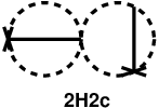
In Table 8, the weak-field expansion of $T_{1}\sim T_{4}$ , the classification of $\partial^{4}h\cdot\partial^{2}h$ -invariants and their weights are given. The total sum of weights is $945=9\times 7\times 5\times 3\times 1$ . We see $T_{i}$ ’s are independent each other.

bridge-	$\underline{l}$	Graph	Weight,	$T_{1}$	$T_{2}$	$T_{3}$	$T_{4}$
no		Name	Total 945
	3	Q’Q	24	1	0	0	0
0	4	Q’P	12	-1	0	0	0
		P’Q	6	-1	0	0	0
	5	P’P	3	1	0	0	0
		2H2a	96	0	${\frac{1}{2}}$	0	0
	2	2H2b	96	0	${\frac{1}{2}}$	0	0
		2H2c	96	0	0	0	1
		3H2a	24	0	$-{\frac{1}{2}}$	0	0
		3H2b	48	0	$-{\frac{1}{2}}$	0	-1
	3	3H2c	48	0	$-{\frac{1}{2}}$	0	0
2		3H2d	48	0	$-{\frac{1}{2}}$	0	0
		3H2e	24	0	0	0	$-{\frac{1}{2}}$
		3H2f	24	0	0	0	$-{\frac{1}{2}}$
		4H2a	6	0	$\frac{1}{4}$	0	0
	4	4H2b	6	0	$\frac{1}{4}$	0	0
		4H2c	12	0	$\frac{1}{4}$	0	${\frac{1}{2}}$
		4H2d	12	0	$\frac{1}{4}$	0	${\frac{1}{2}}$
		2H4a	96	0	0	0	0
	2	2H4b	96	0	0	0	0
4		2H4c	96	0	0	-2	0
		3H4a	24	0	0	0	0
	3	3H4b	24	0	0	1	0
		3H4c	24	0	0	1	0

Table 8: Classification of

\partial^{4}h\cdot\partial^{2}h

-invariants, their weights and weak-field expansion of

\nabla\nabla R\times R

-type general invariants.

Appendix D. Classification of $(\partial\partial\partial h)^{2}$ -Invariants and Weak-Expansion of $\nabla R\times\nabla R$ -terms

The leading order of the weak-field expansion for $\nabla R\times\nabla R$ -type general invariants( $O_{1}\sim O_{4}$ ), is given by a sum of $(\partial\partial\partial h)^{2}$ -invariants. We introduce a graphical representation, in Fig.40, for a 5-tensor $\partial_{\mu}\partial_{\nu}\partial_{\lambda}h_{\alpha\beta}$ .

We list here all and independent $(\partial\partial\partial h)^{2}$ -invariants. bridgeno must be an odd number in this case because the $\partial\partial\partial h$ -tensor has an odd number of suffixes. Especially there are no disconnected graphs. We classify them by bridgeno and $\underline{l}$ , as follows. (i) bridgeno=1 ,Fig.41.
2F1a, 2F1b, 2F1c ( $\underline{l}=2$ ); 3F1a, 3F1b ( $\underline{l}=3$ ); 4F1 ( $\underline{l}=4$ ). (ii) bridgeno=3 , Fig.42.
2F3a, 2F3b, 2F3c, 2F3d, 2F3e ( $\underline{l}=2$ ); 3F3a, 3F3b, 3F3c, 3F3d ( $\underline{l}=3$ ). (iii) bridgeno=5 , Fig.43.
2F5a, 2F5b ( $\underline{l}=2$ ); 3F5 ( $\underline{l}=3$ ).

In Table 9, the weak-field expansion of $O_{1}\sim O_{4}$ , the classification of $(\partial\partial\partial h)^{2}$ -invariants and their weights are given. The total sum of weights is $945=9\times 7\times 5\times 3\times 1$ . We see $O_{i}$ ’s are independent each other.

bridge-	$\underline{l}$	Graph	Weight,	$O_{1}$	$O_{2}$	$O_{3}$	$O_{4}$
no		Name	Total 945
		2F1a	36	0	0	0	0
	2	2F1b	36	1	0	0	0
1		2F1c	72	0	0	0	0
	3	3F1a	36	0	0	0	0
		3F1b	36	-2	0	0	0
	4	4F1	9	1	0	0	0
		2F3a	36	0	0	0	$\frac{1}{4}$
		2F3b	72	0	0	0	$-{\frac{1}{2}}$
	2	2F3c	144	0	-1	0	$-{\frac{1}{2}}$
		2F3d	72	0	${\frac{1}{2}}$	0	$\frac{3}{4}$
3		2F3e	144	0	${\frac{1}{2}}$	0	$\frac{1}{4}$
		3F3a	6	0	$\frac{1}{4}$	0	$\frac{1}{4}$
	3	3F3b	18	0	$\frac{1}{4}$	0	0
		3F3c	36	0	${\frac{1}{2}}$	0	${\frac{1}{2}}$
		3F3d	72	0	-1	0	-1
	2	2F5a	36	0	0	1	0
5		2F5b	72	0	0	-2	0
	3	3F5	12	0	0	1	0

Table 9: Classification of

(\partial\partial\partial h)^{2}

-invariants, their weights and weak-field expansion of

\nabla R\times\nabla R

-type general invariants.

Appendix E. Weak Field Expansion of General Invariants

In this appendix we list the weak expansion of $RRR$ -type general invariants: $P_{1}\sim P_{6},A_{1},B_{1}$ . We focus only in $(\partial\partial h)^{3}$ -terms among different types of expanded terms. The classification of $(\partial\partial h)^{3}$ -invariants is the main theme of the text. The result is most fruitfully utilized in this appendix. Especially the set of indices, which characterizes every $(\partial\partial h)^{3}$ -invariant by its graph topology, is exploited in the (computer) calculation. The following results show the power of the present approach. We see the 8 general invariants are locally independent each other, furthermore they are “orthogonal” in the space of $(\partial\partial h)^{3}$ -invariants except in the “directions” of $G3$ and $G13$ ( $A_{1}$ and $B_{1}$ only are mixed in those “directions”) [22] .

Graph	$P_{1}$	$P_{2}$	$P_{3}$	$P_{4}$	$P_{5}$	$P_{6}$	$A_{1}$	$B_{1}$
$G1$	$0$	$0$	$0$	$-\frac{1}{4}$	$0$	$0$	$0$	$0$
$G2$	$0$	$0$	$0$	$0$	$\frac{1}{4}$	$0$	$0$	$0$
$G3$	$0$	$0$	$0$	$0$	$0$	$0$	$-1$	$-\frac{1}{4}$
$G4$	$0$	$0$	$0$	$-\frac{3}{4}$	$0$	$0$	$0$	$0$
$G5$	$0$	$0$	$0$	$0$	$0$	${\frac{1}{2}}$	$0$	$0$
$G6$	$0$	$0$	$0$	$0$	$0$	${\frac{1}{2}}$	$0$	$0$
$G7$	$0$	$0$	$0$	$0$	$0$	$0$	$0$	$\frac{3}{2}$
$G8$	$0$	$0$	$0$	$0$	${\frac{1}{2}}$	$0$	$0$	$0$
$G9$	$0$	$0$	$0$	$0$	$0$	${\frac{1}{2}}$	$0$	$0$
$G10$	$0$	$0$	$0$	$0$	$\frac{1}{4}$	$0$	$0$	$0$
$G11$	$0$	$0$	$0$	$0$	$0$	${\frac{1}{2}}$	$0$	$0$
$G12$	$0$	$0$	$0$	$0$	$0$	$0$	$0$	$\frac{3}{2}$
$G13$	$0$	$0$	$0$	$0$	$0$	$0$	$-3$	$-\frac{3}{4}$

Table 10: Weak-Expansion of Invariants with

M^{6}

-Dim.:

(\partial\partial h)^{3}

-Part, G1-G13(

\underline{l}

=1)

Graph	$P_{1}$	$P_{2}$	$P_{3}$	$P_{4}$	$P_{5}$	$P_{6}$	$A_{1}$	$B_{1}$
$G14$	$0$	$0$	$0$	$0$	$0$	$0$	$1$	$0$
$G15$	$0$	$0$	$0$	$0$	$0$	$0$	$3$	$0$
$G16$	$0$	$0$	$0$	$0$	$-1$	$0$	$0$	$0$
$G17$	$0$	$0$	$0$	$0$	$0$	$-{\frac{1}{2}}$	$0$	$0$
$G18$	$0$	$0$	$0$	$0$	$0$	$0$	$0$	$-\frac{3}{4}$
$G19$	$0$	$0$	$0$	$0$	$0$	$-{\frac{1}{2}}$	$0$	$0$
$G20$	$0$	$0$	$0$	$0$	$0$	$0$	$0$	$-\frac{3}{4}$
$G21$	$0$	$0$	$0$	$0$	$0$	$-{\frac{1}{2}}$	$0$	$0$
$G22$	$0$	$0$	$0$	$0$	$0$	$0$	$0$	$-\frac{3}{2}$
$G23$	$0$	$-{\frac{1}{2}}$	$0$	$0$	$0$	$0$	$0$	$0$
$G24$	$0$	$0$	$2$	$0$	$0$	$0$	$0$	$0$
$G25$	$0$	$0$	$0$	$0$	$0$	$-{\frac{1}{2}}$	$0$	$0$
$G26$	$0$	$-{\frac{1}{2}}$	$0$	$0$	$0$	$0$	$0$	$0$
$G27$	$0$	$0$	$0$	$\frac{3}{8}$	$0$	$0$	$0$	$0$
$G28$	$0$	$0$	$0$	$0$	$0$	$-\frac{1}{4}$	$0$	$0$
$G29$	$0$	$0$	$0$	$0$	$-{\frac{1}{2}}$	$0$	$0$	$0$
$G30$	$0$	$0$	$0$	$0$	$0$	$-{\frac{1}{2}}$	$0$	$0$
$G31$	$0$	$0$	$0$	$0$	$-{\frac{1}{2}}$	$0$	$0$	$0$
$G32$	$0$	$0$	$0$	$\frac{3}{4}$	$0$	$0$	$0$	$0$
$G33$	$0$	$0$	$0$	$\frac{3}{8}$	$0$	$0$	$0$	$0$
$G34$	$0$	$0$	$0$	$0$	$0$	$-\frac{1}{4}$	$0$	$0$
$G35$	$0$	$0$	$0$	$\frac{3}{8}$	$0$	$0$	$0$	$0$
$G36$	$0$	$0$	$0$	$0$	$0$	$-\frac{1}{4}$	$0$	$0$
$G37$	$0$	$0$	$0$	$0$	$-{\frac{1}{2}}$	$0$	$0$	$0$
$G38$	$0$	$0$	$0$	$0$	$0$	$-{\frac{1}{2}}$	$0$	$0$
$G39$	$0$	$0$	$0$	$\frac{3}{8}$	$0$	$0$	$0$	$0$
$G40$	$0$	$0$	$0$	$0$	$0$	$-\frac{1}{4}$	$0$	$0$
$G41$	$0$	$0$	$0$	$0$	$-{\frac{1}{2}}$	$0$	$0$	$0$
$G42$	$0$	$0$	$0$	$\frac{3}{4}$	$0$	$0$	$0$	$0$

Table 11: Weak-Expansion of Invariants with

M^{6}

-Dim.:

(\partial\partial h)^{3}

-Part, G14-G42(

\underline{l}

=2)

Graph	$P_{1}$	$P_{2}$	$P_{3}$	$P_{4}$	$P_{5}$	$P_{6}$	$A_{1}$	$B_{1}$
$G43$	$0$	$0$	$0$	$0$	$\frac{1}{4}$	$0$	$0$	$0$
$G44$	$0$	$0$	$0$	$-\frac{3}{4}$	$0$	$0$	$0$	$0$
$G45$	$0$	$0$	$0$	$0$	$0$	$\frac{1}{4}$	$0$	$0$
$G46$	$0$	$0$	$0$	$0$	$0$	$\frac{1}{4}$	$0$	$0$
$G47$	$0$	$0$	$0$	$0$	$0$	$\frac{1}{4}$	$0$	$0$
$G48$	$0$	$0$	$0$	$0$	${\frac{1}{2}}$	$0$	$0$	$0$
$G49$	$0$	$0$	$0$	$0$	$0$	$0$	$0$	$\frac{3}{4}$
$G50$	$0$	$0$	$-1$	$0$	$0$	$0$	$0$	$0$
$G51$	$0$	$0$	$0$	$-\frac{3}{4}$	$0$	$0$	$0$	$0$
$G52$	$0$	$0$	$0$	$0$	${\frac{1}{2}}$	$0$	$0$	$0$
$G53$	$0$	${\frac{1}{2}}$	$0$	$0$	$0$	$0$	$0$	$0$
$G54$	$0$	$0$	$-2$	$0$	$0$	$0$	$0$	$0$
$G55$	$0$	$0$	$0$	$-\frac{3}{4}$	$0$	$0$	$0$	$0$
$G56$	$0$	${\frac{1}{2}}$	$0$	$0$	$0$	$0$	$0$	$0$
$G57$	$0$	$0$	$0$	$0$	$0$	$\frac{1}{4}$	$0$	$0$
$G58$	$0$	$0$	$0$	$0$	${\frac{1}{2}}$	$0$	$0$	$0$
$G59$	$0$	$0$	$0$	$0$	$0$	${\frac{1}{2}}$	$0$	$0$
$G60$	$0$	$0$	$0$	$0$	${\frac{1}{2}}$	$0$	$0$	$0$
$G61$	$0$	$1$	$0$	$0$	$0$	$0$	$0$	$0$
$G62$	$0$	$0$	$0$	$-\frac{3}{4}$	$0$	$0$	$0$	$0$
$G63$	$0$	$0$	$0$	$0$	$\frac{1}{4}$	$0$	$0$	$0$
$G64$	$0$	$0$	$0$	$0$	$0$	${\frac{1}{2}}$	$0$	$0$
$G65$	$0$	$0$	$0$	$0$	${\frac{1}{2}}$	$0$	$0$	$0$
$G66$	$0$	$1$	$0$	$0$	$0$	$0$	$0$	$0$
$G67$	$0$	$0$	$0$	$0$	$0$	$0$	$0$	$\frac{1}{4}$
$G68$	$0$	$0$	$-1$	$0$	$0$	$0$	$0$	$0$
$G69$	$-1$	$0$	$0$	$0$	$0$	$0$	$0$	$0$

Table 12: Weak-Expansion of Invariants with

M^{6}

-Dim.:

(\partial\partial h)^{3}

-Part ,G43-G69(

\underline{l}

=3)

Graph	$P_{1}$	$P_{2}$	$P_{3}$	$P_{4}$	$P_{5}$	$P_{6}$	$A_{1}$	$B_{1}$
$G70$	$0$	$0$	$0$	$\frac{1}{8}$	$0$	$0$	$0$	$0$
$G71$	$0$	$0$	$0$	$0$	$-\frac{1}{4}$	$0$	$0$	$0$
$G72$	$0$	$0$	$1$	$0$	$0$	$0$	$0$	$0$
$G73$	$0$	$0$	$0$	$\frac{3}{8}$	$0$	$0$	$0$	$0$
$G74$	$0$	$-1$	$0$	$0$	$0$	$0$	$0$	$0$
$G75$	$0$	$0$	$0$	$0$	$-\frac{1}{4}$	$0$	$0$	$0$
$G76$	$0$	$-\frac{1}{4}$	$0$	$0$	$0$	$0$	$0$	$0$
$G77$	$0$	$0$	$0$	$\frac{1}{8}$	$0$	$0$	$0$	$0$
$G78$	$0$	$0$	$0$	$0$	$-\frac{1}{4}$	$0$	$0$	$0$
$G79$	$0$	$-\frac{1}{4}$	$0$	$0$	$0$	$0$	$0$	$0$
$G80$	$0$	$0$	$0$	$\frac{3}{8}$	$0$	$0$	$0$	$0$
$G81$	$0$	$-1$	$0$	$0$	$0$	$0$	$0$	$0$
$G82$	$0$	$0$	$0$	$0$	$-\frac{1}{4}$	$0$	$0$	$0$
$G83$	$0$	$-{\frac{1}{2}}$	$0$	$0$	$0$	$0$	$0$	$0$
$G84$	$0$	$0$	$1$	$0$	$0$	$0$	$0$	$0$
$G85$	$3$	$0$	$0$	$0$	$0$	$0$	$0$	$0$
$G86$	$0$	$\frac{1}{4}$	$0$	$0$	$0$	$0$	$0$	$0$
$G87$	$0$	$\frac{1}{4}$	$0$	$0$	$0$	$0$	$0$	$0$
$G88$	$-3$	$0$	$0$	$0$	$0$	$0$	$0$	$0$
$G89$	$0$	${\frac{1}{2}}$	$0$	$0$	$0$	$0$	$0$	$0$
$G90$	$1$	$0$	$0$	$0$	$0$	$0$	$0$	$0$

Table 13: Weak-Expansion of Invariants with

M^{6}

-Dim.:

(\partial\partial h)^{3}

-Part ,G70-G85(

\underline{l}

=4),G86-G89(

\underline{l}

=5),G90(

\underline{l}

=6)

Appendix F. Graphs of General Invariants with $M^{6}$ Dimension

In this section we graphically list all independent (in n-dim space) general invariants with $M^{6}$ dimension. They are classified in the following ways.

(i) Fig.44: $RRR$ -type (on-shell vanishing)

(ii) Fig.45: $RRR$ -type (on-shell non-vanishing)

(iii) Fig.46: $\nabla\nabla R\times R$ -type

(iv) Fig.47: $\nabla R\times\nabla R$ -type

(v) Fig.48: $\nabla^{2}\nabla^{2}R$ -type

Appendix G. Graphical Definitions of Totally Anti-symmetrized Quantities

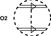
All independent non-vanishing totally anti-symmetrized quantities with the dimension $M^{6}$ are graphically defined in this appendix. They are used, in Sec.IX of the text, to derive special relations, between general invariants, valid only in each dimension. The anti-symmetrized quantities are grouped, in the following, by the type of a starting general invariant: Fig.49-51 ( $R\times R\times R$ -type), Fig.52 ( $\nabla\nabla R\times R$ -type) and Fig.53( $\nabla R\times\nabla R$ -type).

References

[1] On leave of absence, until Jan. 31,1997, from Department of Physics, University of Shizuoka, Yada 52-1, Shizuoka 422, Japan. E-mail address: s.ichinose@damtp.cam.ac.uk ; ichinose@momo1.u-shizuoka-ken.ac.jp
[2] E-mail address: nori@kurims.kyoto-u.ac.jp
[3] S.A.Fulling, R.C.King, B.G.Wybourne and C.J.Cummins, Class.Quantum Grav.,9,1151(1992)
[4] S.Ichinose,Class.Quantum Grav.12,1021(1995).
[5] When we say “dimension”, there are two different meanings in this paper. One is the dimension of space, which we call the space-dimension when clear separation is necessary. The other is the mass dimension of an operator. For example, the Riemann tensor has an $M^{2}$ dimension in any space-dimension. We call it the mass-dimension when necessary.
[6] The relations come from “Type 2” symmetry in Sec.2 of [4]. Note that the statement does not apply to those relations which come from “Type 3” symmetry. It is the symmetry depending on each dimension.
[7] S.Ichinose and N.Ikeda,Preprint of Univ. of Shizuoka, US-96-03,1996, ’Weak Field Expansion of Gravity and Graphical Representation’
[8] bcn[ ] imply an general element of an array:bcn[0], $\cdots$ ,bcn[ $\underline{l}$ ]. The same thing is for vcn[ ]. All quantities of indices are underlined in the following.
[9] The introduced indices here are the same as those explained in Lemma of Sec.II: ddverno[ $i$ ]= $w_{i}$ ,hverno[ $i$ ]= $v_{i}$ .
[10] As a general tendency, we see, from the result of App.B, the weight of a graph decreases as its suffix-loop no ( $l$ ) increases.
[11] In contrast with [4], we take here double solid lines to express the ’bond’ of $R_{{\mu\nu}{\lambda\sigma}}$ in order to avoid the confusion with $\partial_{\mu}\partial_{\nu}h_{\alpha\beta}$ of Fig.1.
[12] P.B.Gilkey,Jour.Diff.Geom.10,601(1975).
[13] L.Bonora,P.Pasti and M.Bregola,Class.Quantum Grav.3,635(1986).
[14] Note that in [4], total derivative terms are neglected, whereas they are not neglected in the present case.
[15] { $P_{1}-P_{6}$ }, $A_{1}$ , $B_{1}$ and { $O_{1}-O_{2}$ } are the same notation as that in [4]. $O_{3}$ and $O_{4}$ in (258) correspond to $Q_{2}$ and $Q_{10}$ in [4] respectively.(There is a typographical mistake in the figure caption of Fig.15 of [4] where a minus sign is missing in the literal (not graphical) definition of $P_{5}$ . The one given in (258) of the present text is the right one.)
[16] M.H.Goroff and A.Sagnotti,Nucl.Phys.B266,709(1986).
[17] S.Deser and A.Schwimmer,Phys.Lett.B309,279(1993).
[18] R.Kallosh,Nucl.Phys.B78,293(1974).
[19] P.van Nieuwenhuizen and C.C.Wu,J.Math.Phys.18,182(1877)
[20] The space-dimension is taken to be 2 in order to obtain the mass-dimensions of the couplings, (282), without introducing any additional mass parameters. Note that the present purpose is the graph classification. There the important thing is the topological structure of graphs. The space-dimension of the field theory is irrelevant.
[21] S.Ichinose and N.Ikeda, hep-th/9509073, Phys.Rev.D53,5932(1996)
[22] Among 90 terms listed in App.A, G3 and G13 only has the crossing number 3. As for the definition of the crossing number, see Subsec.V.ii.

Figure Captions

•

Fig.1 4-tensor $\partial_{\mu}\partial_{\nu}h_{\alpha\beta}$
•

Fig.2 Graphical representation of $A1=\partial_{\sigma}\partial_{\lambda}h_{\mu\nu}\cdot\partial_{\sigma}\partial_{\nu}h_{\mu\lambda}$ .
•

Fig.3 Bondless diagram for $A1$ of Fig.2. dd-vertices are explicitly represented by small circles.
•

Fig.4 Graphical representation of $PQ=\partial^{2}h_{\lambda\lambda}\cdot\partial_{\mu}\partial_{\nu}h_{{\mu\nu}}$ .
•

Fig.5 Bondless diagrams and values of ( $v$ , $w$ , vcn).
•

Fig.6 Reduction procedure of identifying two vertex-types: dd-vertex and h-vertex.
•

Fig.7 Classification of $(\partial\partial h)^{3}$ -graphs by bcn[ ], $\underline{l}=1$ .
•

Fig.8 Classification of $(\partial\partial h)^{3}$ -graphs by bcn[ ], $\underline{l}=2$ .
•

Fig.9 Classification of $(\partial\partial h)^{3}$ -graphs by bcn[ ], $\underline{l}=3$ .
•

Fig.10 Classification of $(\partial\partial h)^{3}$ -graphs by bcn[ ], $\underline{l}=4$ .
•

Fig.11 Reduction of Graphs.
•

Fig.12 Reduced Graphs by the procedure Fig.8.
•

Fig.13 G51: $3F_{a}\Theta$ .
•

Fig.14 Three Graphs with the same $\underline{l}$ ,vcn and bcn. Vorder discriminate them.
•

Fig.15 Two Graphs (G28,G30) with the same $\underline{l}$ ,vcn[ ] and bcn[ ]. Vorder discriminate them.
•

Fig.16 Two Graphs with the same $\underline{l}$ ,vcn[ ] and bcn[ ]. ddverno[ ] and hverno[ ] discriminate them.
•

Fig.17 Two Graphs with the same $\underline{l}$ ,vcn and bcn. crossno[ ] discriminates them.
•

Fig.18 Vertices and propagators of (253).
•

Fig.19 Vertices and propagators of (254).
•

Fig.20 The vertex of (255).
•

Fig.21 Graphical representations for (a) $R_{{\mu\nu}{\lambda\sigma}}$ , (b) $\nabla_{\alpha}R_{{\mu\nu}{\lambda\sigma}}$ and (c) $\nabla_{\alpha}\nabla_{\beta}R_{{\mu\nu}{\lambda\sigma}}$ .
•

Fig.22 Graphical representation for the Riemann scalar $R$ .
•

Fig.23 Graphical representation for (a) $\nabla^{2}R$ , (b) $R^{2}$ , (c) $R_{\mu\nu}R^{\mu\nu}$ , and (d) $R_{{\mu\nu}{\lambda\sigma}}R^{{\mu\nu}{\lambda\sigma}}$ .
•

Fig.24 Graphical representation for $I^{an2}_{R}\equiv R^{{\alpha\beta}}_{~\beta\alpha}-R^{\alpha\beta}_{~{\alpha\beta}}$ . In the figure, anti[ $\alpha,\beta$ ] means anti-symmetrization w.r.t. $\alpha$ and $\beta$ . The second-line figure demonstrates the present notation used in the following.
•

Fig.25 Graphical definition for $I^{an3}_{RR}$ and $I^{an4}_{RR}$ . In the figure, anti[ $\alpha,\beta,\gamma$ ] and anti[ $\alpha,\beta,\gamma,\delta$ ] mean totally anti-symmetrization w.r.t. ( $\alpha,\beta,\gamma$ ) and ( $\alpha,\beta,\gamma,\delta$ ) respectively.
•

Fig.26 (i) $\underline{l}=1$ ( 13(con)+0(discon)=13 terms G1-13.
•

Fig.27 (ii) $\underline{l}=2$ ( 26(con)+3(discon)=29 terms G14-42 No.1
•

Fig.28 (ii) $\underline{l}=2$ ( 26(con)+3(discon)=29 terms G14-42 No.2
•

Fig.29 (iii) $\underline{l}=3$ ( 19(con)+8(discon)=27 terms G43-69 No.1
•

Fig.30 (iii) $\underline{l}=3$ ( 19(con)+8(discon)=27 terms G43-69 No.2
•

Fig.31 (iv) $\underline{l}=4$ ( 8(con)+8(discon)=16 terms G70-85, No.1
•

Fig.32 (iv) $\underline{l}=4$ ( 8(con)+8(discon)=16 terms G70-85, No.2
•

Fig.33 (v) $\underline{l}=5$ ( 0(con)+4(discon)=4 terms, G86-89
•

Fig.34 (vi) $\underline{l}=6$ ( 0(con)+1(discon)=1 term, G90
•

Fig.35 Graphs of 6-tensor $\partial_{\mu}\partial_{\nu}\partial_{\lambda}\partial_{\sigma}h_{\alpha\beta}$
•

Fig.36 Graphs for $P^{\prime}\equiv\partial^{2}\partial^{2}h_{\mu\mu}$ and $Q^{\prime}\equiv\partial^{2}\partial_{\mu}\partial_{\nu}h_{\mu\nu}$ .
•

Fig.37 Graphs for bridgeno=0 ( disconnected )
•

Fig.38 Graphs for bridgeno=2
•

Fig.39 Graphs for bridgeno=4
•

Fig.40 Graphs of 5-tensor $\partial_{\mu}\partial_{\nu}\partial_{\lambda}h_{\alpha\beta}$
•

Fig.41 Graphs for bridgeno=1
•

Fig.42 Graphs for bridgeno=3
•

Fig.43 Graphs for bridgeno=5
•

Fig.44 Graphs for $P_{1}=RRR{\quad,}\ \ P_{2}=RR_{\mu\nu}R^{\mu\nu},P_{3}=RR_{{\mu\nu}{\lambda\sigma}}R^{{\mu\nu}{\lambda\sigma}},P_{4}=R_{\mu\nu}R^{\nu\lambda}R_{\lambda}^{~\mu},P_{5}=R_{{\mu\nu}{\lambda\sigma}}R^{\mu\lambda}R^{\nu\sigma}$ and $P_{6}=R_{{\mu\nu}{\lambda\sigma}}R_{\tau}^{~\nu{\lambda\sigma}}R^{\mu\tau}$ .
•

Fig.45 Graphs for $A_{1}=R_{{\mu\nu}{\lambda\sigma}}R^{\sigma\lambda}_{~~~\tau\omega}R^{\omega\tau\nu\mu}$ and $B_{1}=R_{{\mu\nu}\tau\sigma}R^{\nu~~~\tau}_{~\lambda\omega}R^{\lambda\mu\sigma\omega}$ .
•

Fig.46 Graphs for $T_{1}=\nabla^{2}R\cdot R,T_{2}=\nabla^{2}R_{\lambda\sigma}\cdot R^{\lambda\sigma},T_{3}=\nabla^{2}R_{\lambda\rho\sigma\tau}\cdot R^{\lambda\rho\sigma\tau}$ , and $T_{4}=\nabla^{\mu}\nabla^{\nu}R\cdot R_{\mu\nu}$ .
•

Fig.47 Graphs for $O_{1}=\nabla^{\mu}R\cdot\nabla_{\mu}R,O_{2}=\nabla^{\mu}R_{\lambda\sigma}\cdot\nabla_{\mu}R^{\lambda\sigma},O_{3}=\nabla^{\mu}R^{\lambda\rho\sigma\tau}\cdot\nabla_{\mu}R_{\lambda\rho\sigma\tau}$ , and $O_{4}=\nabla^{\mu}R_{\lambda\nu}\cdot\nabla^{\nu}R^{\lambda}_{~\mu}$ .
•

Fig.48 Graphs for $S=\nabla^{2}\nabla^{2}R$ .
•

Fig.49 Graphical definition for $I^{an3}_{P_{1}},I^{an3}_{A_{1}},I^{an3}_{P_{3}},I^{an3}_{B_{1}(a)},I^{an3}_{B_{1}(b)}$ and $I^{an3}_{P_{5}}$ .
•

Fig.50 Graphical definition for $I^{an4}_{P_{1}},I^{an4}_{A_{1}},I^{an4}_{P_{3}}$ and $I^{an4}_{P_{6}}$ .
•

Fig.51 Graphical definition for $I^{an5}_{P_{1}},I^{an5}_{A_{1}}$ and $I^{an6}_{P_{1}}$ .
•

Fig.52 Graphical definition for $I^{an3}_{T_{1}(a)},I^{an3}_{T_{1}(b)},I^{an3}_{T_{1}(c)},I^{an3}_{T_{3}},I^{an4}_{T_{1}(a)}$ and $I^{an4}_{T_{1}(b)}$ .
•

Fig.53 Graphical definition for $I^{an3}_{O_{1}(a)},I^{an3}_{O_{1}(b)}$ and $I^{an4}_{O_{1}}$ .

G1: $1A\Theta$	G2: $1A\Xi$	G3: $1A\Omega_{2}$
G4: $1B\Theta$	G5: $1B\Sigma-a$	G6: $1B\Sigma-b$
G7: $1B\Omega_{1}$	G8: $1B\Xi$	G9: $1B\Sigma-c$
G10: $1C\Xi$	G11: $1C\Sigma$	G12: $1C\Omega_{1}$
G13: $1C\Omega_{2}$

G14: $2A\Omega_{1}$	G15: $2D\Omega_{1}$	G16: $2D\Xi_{1}$
G17: $2B\Sigma_{1}$	G18: $2B\Omega_{2}$	G19: $2C\Sigma_{1}$
G20: $2C\Omega_{2}$	G21: $2E_{a}\Sigma_{1}$	G22: $2E_{a}\Omega_{2}$
G23: $A2Q$	G24: $A1Q$	G25: $2E_{b}\Sigma_{1}$
G26: $A3Q$	G27: $2F_{a}\Theta$	G28: $2F_{a}\Sigma_{2}-a$

G29: $2F_{a}\Xi_{2}$	G30: $2F_{a}\Sigma_{2}-b$	G31: $2F_{b}\Xi_{2}$
G32: $2F_{b}\Theta-a$	G33: $2F_{b}\Theta-b$	G34: $2F_{b}\Sigma_{2}$
G35: $2G_{a}\Theta$	G36: $2G_{a}\Sigma_{2}-a$	G37: $2G_{a}\Xi_{2}$
G38: $2G_{a}\Sigma_{2}-b$	G39: $2G_{b}\Theta-a$	G40: $2G_{b}\Sigma_{2}$
G41: $2G_{b}\Xi_{2}$	G42: $2G_{b}\Theta-b$

G43: $3A\Xi_{1}$	G44: $3A\Theta$	G45: $3B\Sigma$
G46: $3C\Sigma$	G47: $3D\Sigma$	G48: $3D\Xi_{2}$
G49: $3E\Omega$	G50: $B3Q$	G51: $3F_{a}\Theta$
G52: $3F_{a}\Xi_{1}$	G53: $A2P$	G54: $A1P$
G55: $3F_{b}\Theta$	G56: $A3P$	G57: $3G\Sigma$
G58: $3G\Xi_{2}$	G59: $3H\Sigma$	G60: $3H\Xi_{2}$
G61: $B2Q$	G62: $3I\Theta$	G63: $3I\Xi_{1}$

G64: $3J\Sigma$	G65: $3J\Xi_{2}$	G66: $B1Q$
G67: $3K\Omega$	G68: $B4Q$	G69: $QQQ$

G70: $4A\Theta$	G71: $4B\Xi$	G72: $B3P$
G73: $4C\Theta$	G74: $B2P$	G75: $4D\Xi$
G76: $C2Q$	G77: $4E\Theta$	G78: $4F\Xi$
G79: $C1Q$	G80: $4G\Theta$	G81: $B1P$

Abstract

I Introduction

II Graphical Representation of SO(n)-Invariants

III Classification of (∂∂⁡h)3(\partial\partial h)^{3}-Invariants by Bondless Diagrams

IV Classification of (∂∂⁡h)3(\partial\partial h)^{3}-Invariants by Reduced Graphs

V Indices of (∂∂⁡h)3(\partial\partial h)^{3}-Invariants

V.i Tadpole Number and Type of Tadpole

V.ii Indices for Discriminating ’Fine Structure’ of (∂∂⁡h)3(\partial\partial h)^{3}-Invariants

VI Identities between Weights

VII Disconnected part

VIII Independence of General Invariants

VIII.i Graphical Representation of General Tensors and Invariants

VIII.ii Independent General Invariants as Local Functions

IX Relations Valid for Only Each Dimension

X Discussions and Conclusions

References

III Classification of $(\partial\partial h)^{3}$ -Invariants by Bondless Diagrams

IV Classification of $(\partial\partial h)^{3}$ -Invariants by Reduced Graphs

V Indices of $(\partial\partial h)^{3}$ -Invariants

V.ii Indices for Discriminating ’Fine Structure’ of $(\partial\partial h)^{3}$ -Invariants