IC/2006/131
NSF-KITP-06-117
MCTP-06-34
Explaining the Electroweak Scale and Stabilizing Moduli in theory
Abstract
In a recent paper Acharya:2006ia it was shown that in fluxless theory vacua with at least two hidden sectors undergoing strong gauge dynamics and a particular form of the Kähler potential, all moduli are stabilized by the effective potential and a stable hierarchy is generated, consistent with standard gauge unification. This paper explains the results of Acharya:2006ia in more detail and generalizes them, finding an essentially unique de Sitter (dS) vacuum under reasonable conditions. One of the main phenomenological consequences is a prediction which emerges from this entire class of vacua: namely gaugino masses are significantly suppressed relative to the gravitino mass. We also present evidence that, for those vacua in which the vacuum energy is small, the gravitino mass, which sets all the superpartner masses, is automatically in the TeV - 100 TeV range.
I Introduction and Summary
There are many good reasons why we study string theory as a theory of particle physics. One of these, discovered some twenty or so years ago Candelas:1985en, is that a simple question, “what properties do four-dimensional heterotic string vacua generically have?” has an extremely compelling answer: non-Abelian gauge symmetry, chiral fermions, hierarchical Yukawa couplings and dynamical supersymmetry breaking. One can also add other important properties such as gauge coupling unification and doublet-triplet splitting. Furthermore, after the dust of the string duality revolution settled, a similar picture was discovered in other perturbative corners of the landscape, eg Type IIA, Type IIB and theory. The above four properties are the most important properties of the Standard Model. The fifth one - gauge coupling unification - is an important feature of the MSSM and low energy supersymmetry.
There is another crucial feature of the Standard Model: namely its overall mass scale, which is of order as opposed to some other scale such as or . This property of the Standard Model is much less well understood in string theory or otherwise, and will be the focus of this paper.
In string/ theory, masses and coupling constants, including are all functions of the moduli field vevs. Thus the hierarchy problem in string theory is double edged: one has to both stabilize all the moduli and generate the hierarchy simultaneously. In recent years there has been progress in moduli stabilization via fluxes and other effects (for a recent review see Douglas:2006es), and with the imminent arrival of the LHC it is appropriate to address the hierarchy problem in this context. After all, any given string/ theory vacuum either will or will not be consistent with the LHC signal, but one cannot even begin to address this in a meaningful way if the hierarchy is not understood.
In Type IIB vacua, moduli are stabilized via a combination of fluxes and quantum corrections Giddings:2001yu; Kachru:2003aw. In these vacua, hierarchies arise in three ways: warp factors Giddings:2001yu; Verlinde:1999fy as in Randall:1999ee, the presence of non-perturbative effects Kachru:2003aw or by fine tuning the large number of fluxes. However, flux vacua in Type IIA DeWolfe:2005uu, theory Acharya:2002kv and heterotic string theory Gukov:2003cy have the property that the (currently known and understood) fluxes roughly are equal in number to the number of moduli. This leads to a large value of the superpotential, and consequently, if the volume of the extra dimensions is not huge, to a large gravitino mass. This tends to give a large mass to all scalars via the effective 4d supergravity potential, which leads to either or some other large value such as or . Therefore, for these vacua we require a good idea for generating and stabilizing the hierarchy.
Thus far, there has been essentially one good idea proposed to explain the relatively small value of the weak scale. This is that the weak scale might be identified with, or related to, the strong coupling scale of an asymptotically free theory which becomes strongly coupled at low energies and exhibits a mass gap at that strong coupling scale. Holographically dual to this is the idea of warped extra dimensions Randall:1999ee. Strong dynamics (or its dual) can certainly generate a small scale in a natural manner, but can it also be compatible with the stabilization of all the moduli fields?
One context for this question, which we will see is particularly natural, is theory compactification on manifolds of -holonomy without fluxes. In these vacua, the only moduli one has are zero modes of the metric on , whose bosonic superpartners are axions. Thus each moduli supermultiplet has a Peccei-Quinn shift symmetry (which originates from 3-form gauge transformations in the bulk 11d supergravity). Since such symmetries can only be broken by non-perturbative effects, the entire moduli superpotential is non-perturbative. In general can depend on all the moduli. Therefore, in addition to the small scale generated by the strong dynamics we might expect that all the moduli are actually stabilized. This paper will demonstrate in detail that this is indeed the case.
Having established that the basic idea works well, the next question we address is “what are the phenomenological implications?” Since string/ theory has many vacua, it would be extremely useful if we could obtain a general prediction from all vacua or at least some well-defined subset of vacua. Remarkably, we are able to give such a prediction for all fluxless theory vacua within the supergravity approximation11 1 to which we are restricted for calculability with at least two hidden sectors undergoing strong gauge dynamics and a particular form of the Kähler potential as in (1): gaugino masses are generically suppressed relative to the gravitino mass.
A slightly more detailed elucidation of this result is that in all de Sitter vacua within this class, gaugino masses are always suppressed. In AdS vacua - which are obviously less interesting phenomenologically - the gaugino masses are suppressed in ‘most’ of the vacua. This will be explained in more detail later.
The reason why we are able to draw such a generic conclusion is the following: any given non-perturbative contribution to the superpotential depends on various constants which are determined by a specific choice of -manifold . These constants determine entirely the moduli potential. They are given by the constants which are related to the one-loop beta-function coefficients, the normalization of each term and the constants (see (2)) which characterize the Kähler potential for the moduli. Finally, there is a dependence on the gauge kinetic function, and in theory this is determined by a set of integers which specify the homology class of the 3-cycle on which the non-Abelian gauge group is localized. Rather than study a particular which fixes a particular choice for these constants we have studied the effective potential as a function of the . The result of gaugino mass suppression holds essentially for arbitrary values of the , at least in the supergravity regime where we have been able to calculate. Thus, any -manifold which has hidden sectors with strong gauge dynamics will lead to suppressed gaugino masses.
At a deeper level, however, the reason that this works is that the idea of strong gauge dynamics to solve the hierarchy problem is a good and simple idea which guides us to the answers directly. If one’s theory does not provide a simple mechanism for how the hierarchy is generated, then it is difficult to see how one could obtain a reliable prediction for, say, the spectrum of beyond the Standard Model particles. In a particular subset of Type IIB compactifications, Conlon and Quevedo have also discovered some general results Conlon:2006us. In fact, they remarkably also find that gaugino masses are suppressed at tree level, though the nature of the suppression is not quite the same. Some heterotic compactifications also exhibit a suppression of tree-level gaugino masses Binetruy:2000md.
The suppression of gaugino masses relative to applies for all vacua in the supergravity regime arising out of these compactifications, independent of the value of . However, in a generic vacuum the cosmological constant is too large. If we therefore consider only those vacua in which the cosmological constant is acceptable at leading order, this constrains the scale of further. Remarkably, we find evidence that for such vacua, is of order TeV. This result certainly deserves much further investigation.
The fact that such general results emerge from these studies makes the task of predicting implications for various collider observables as well as distinguishing among different vacua with data from the LHC (or any other experiment) easier. A more detailed study of the collider physics and other phenomenology will appear in the future ToAppear. However, as we will see in section VIII, it could be quite easy to distinguish Type IIB and theory vacua using the forthcoming LHC data.
This paper is the somewhat longer companion paper to Acharya:2006ia. Given its length we thought that it would be worthwhile to end this introduction with a guide to its contents. Much of the bulk of the paper is devoted to analyzing and explaining the details of why the potential generated by strong dynamics in the hidden sector has vacua in which all moduli are stabilized. At first we begin with the simplest non-trivial example, two hidden sectors, without any charged matter: only gauge bosons and gauginos. Section II calculates the moduli potential in this case. Section III analyzes its supersymmetric vacua: these are all isolated with a negative vacuum energy. Section IV describes explicit examples realizing the vacuum structure of Sections III and V. Section V describes the vacua which spontaneously break supersymmetry. These also have negative vacuum energy and all moduli stabilized. Section VI goes on to consider more complicated hidden sectors, where it is argued that metastable de Sitter vacua can also occur under very reasonable conditions, and that the metastable de Sitter vacuum obtained for a given -manifold is essentially unique. In section VII we study the distribution of . In particular for the de Sitter vacua it is shown that requiring the absence of a large cosmological constant fixes the gravitino mass to be of (1-100) TeV. Section VIII discusses phenomenology. In particular, we explain the suppression of gaugino masses and discuss the other soft SUSY breaking couplings. We conclude in section IX, followed by an Appendix which discusses the Kähler metric for visible charged matter fields in theory.
II The Moduli Potential
In this section we quickly summarize the basic relevant features of -compactifications, setup the notation and calculate the potential for the moduli generated by strong hidden sector gauge dynamics.
In theory compactifications on a manifold of -holonomy the moduli are in correspondence with the harmonic 3-forms. Since there are such independent 3-forms there are moduli . The real parts of these moduli are axion fields which originate from the 3-form field in theory and the imaginary parts are zero modes of the metric on and characterize the size and shape of . Roughly speaking, one can think of the ’s as measuring the volumes of a basis of the independent three dimensional cycles in .
Non-Abelian gauge fields are localized on three dimensional submanifolds of along which there is an orbifold singularity Acharya:1998pm while chiral fermions are localized at point-like conical singularities Atiyah:2001qf; Acharya:2004qe; Acharya:2001gy. Thus these provide theory realizations of theories with localized matter. A particle localized at a point will be charged under a gauge field supported on if . Since generically, two three dimensional submanifolds do not intersect in a seven dimensional space, there will be no light matter fields charged under both the standard model gauge group and any hidden sector gauge group. Supersymmetry breaking is therefore gravity mediated in these vacua.22 2 This is an example of the sort of general result one is aiming for in string/ theory. We can contrast this result with Type IIA vacua. Here the non-Abelian gauge fields are again localized on 3-cycles, but since generically a pair of three cycles intersect at points in six extra dimensions, In Type IIA supersymmetry breaking will generically be gauge mediated.
In general the Kähler potentials for the moduli are difficult to determine in these vacua. However a set of Kähler potentials, consistent with -holonomy and known to describe accurately some explicit examples of moduli dynamics were given in Acharya:2005ez. These models are given by
| (1) |
where the volume in 11-dimensional units as a function of is
| (2) |
We will assume that this -parameter family of Kähler potentials represents well the moduli dynamics. More general Kähler potentials outside this class have the volume functional multiplied by a function invariant under rescaling of the metric. It would be extremely interesting to investigate the extension of our results to these cases.
As motivated in the introduction, we are interested in studying moduli stabilization induced via strong gauge dynamics. We will begin by considering hidden sector gauge groups with no chiral matter. Later sections will describe the cases with hidden sector chiral matter.
In this ‘no matter’ case, a superpotential (in units of ) of the following form is generated
| (3) |
where is the number of hidden sectors undergoing gaugino condensation, with being the dual coxeter numbers of the hidden sector gauge groups, and are numerical constants. The are RG-scheme dependent and also depend upon the threshold corrections to the gauge couplings; the work of Friedmann:2002ty shows that their ratios (which should be scheme independent) can in fact take a reasonably wide range of values in the space of theory vacua. We will only consider the ratios to vary from (0.1-10) in what follows.
The gauge coupling functions for these singularities are integer linear combinations of the , because a 3-cycle along which a given non-Abelian gauge field is localized is a supersymmetric cycle, whose volume is linear in the moduli.
| (4) |
Notice that, given a particular -manifold for the extra dimensions, the constants are determined. Then, the Kähler potential and superpotential for that particular are completely determined by the constants . This is as it should be, since theory has no free dimensionless parameters.
We are ultimately aiming for an answer to the question, “do theory vacua in general make a prediction for the beyond the standard model spectrum?”. For this reason, since a fluxless theory vacuum is completely specified by the constants we will try as much as possible to pick a particular value for the constants and try to first evaluate whether or not there is a prediction for general values of the constants. Our results will show that at least within the supergravity approximation there is indeed a general prediction: the suppression of gaugino masses relative to the gravitino mass.
At this point the simplest possibility would be to consider a single hidden sector gauge group. Whilst this does in fact stabilize all the moduli, it is a) non-generic and b) fixes the moduli in a place which is strictly beyond the supergravity approximation. Therefore we will begin, for simplicity, by considering two such hidden sectors, which is more representative of a typical compactification as well as being tractable enough to analyze. The superpotential therefore has the following form
| (5) |
The metric corresponding to the Kähler potential (1) is given by
| (6) |
The supergravity scalar potential given by
| (7) |
where
| (8) |
can now be computed. The full expression for the scalar potential is given by
| (9) | |||||
where we introduced a variable
| (10) |
such that
| (11) |
By extremizing (9) with respect to the axions we obtain an equation
| (12) |
which fixes only one linear combination of the axions. In this case
| (13) |
It turns out that in order for the potential (9) to have minima, the axions must take on the values such that for . Otherwise the potential has a runaway behavior. After choosing the minus sign, the potential takes the form
| (14) | |||
In the next section we will go on to analyze the vacua of this potential with unbroken supersymmetry. The vacua in which supersymmetry is spontaneously broken are described in sections V and VI.
III Supersymmetric Vacua
In this section we will discuss the existence and properties of the supersymmetric vacua in our theory. This is comparatively easy to do since such vacua can be obtained by imposing the supersymmetry conditions instead of extremizing the full scalar potential (14). Therefore, we will study this case with the most detail. Experience has also taught us that potentials possessing rigid isolated supersymmetric vacua, also typically have other non-supersymmetric vacua with many qualitatively similar features.
The conditions for a supersymmetric vacuum are:
which implies
| (15) |
Equating the imaginary part of (III) to zero, one finds that
| (16) |
For , a solution with positive values for the moduli () exists when the axions take on the values such that . Now, equating the real part of (III) to zero, one obtains
| (17) |
This is a system of transcendental equations with unknowns. As such, it can only be solved numerically, in which case, it is harder to get a good understanding of the nature of solutions obtained. Rather than doing a brute force numerical analysis of the system (17) it is very convenient to introduce a new auxiliary variable to recast (17) into a system of linear equations with unknowns coupled to a single transcendental constraint as follows:
| (18) | |||
| (19) |
The system of linear equations (18) can then be formally solved for in terms of and :
| (20) |
One can then substitute the solutions for into the constraint (19) and self-consistently solve for the parameter in terms of the input quantities . This, of course, has to be done numerically, but we have indeed verified that solutions exist. Thus, we have shown explicitly that the moduli can be stabilized. We now go on to discuss the solutions, in particular those which lie within the supergravity approximation.
III.1 Solutions and the Supergravity Approximation
Not all choices of the constants lead to solutions consistent with the approximation that in the bulk of spacetime, eleven dimensional supergravity is valid. Although this is not a precisely (in the numerical sense) defined approximation, a reasonable requirement would seem to be that the values of the stabilized moduli () obtained from (20) are greater than 1. It is an interesting question, certainly worthy of further study, whether or not this is the correct criterion. In any case, this is the criterion that we will use and discuss further.
From (20) and (19), and requiring the to be greater than 1, we get the following two branches of conditions on parameter :
| (21) |
Notice that the solution for (20) has a singularity at . This can be seen clearly from Figure (1). We see that the modulus falls very rapidly as one moves away from the vertical asymptote representing the singularity and can become smaller than one very quickly, where the supergravity approximation fails to be valid.

The relative location of the singularities for different moduli will turn out to be very important as we will see shortly. From (21), we know that there are two branches for allowed values of . Here we consider branch a) for concreteness, branch b) can be analyzed similarly.
 |
 |
Right - Positive for the same case plotted as functions of . is represented by the solid curve, by the long dashed curve and by the short dashed curve.The vertical lines again represent the loci of singularities of (20) which the respective moduli asymptote to. The horizontal solid (red) line shows the value unity for the moduli, below which the supergravity approximation is not valid.
Both plots are for .
Figure (2) shows plots for and as functions of for a case with two condensates and three bulk moduli. The plots are for a given choice of the constants . The qualitative feature of the plots remains the same even if one has a different value for the constants.
Since the fall very rapidly as one goes to the left of the vertical asymptotes, there is a small region of between the origin and the leftmost vertical asymptote which yields allowed values for all . Thus, for a solution in the supergravity regime all (three) vertical lines representing the loci of singularities of the (three) moduli should be (sufficiently) close to each other. This means that the positions of the vertical line for the th modulus () and the th modulus () can not be too far apart. This in turn implies that the ratio of integer coefficients and for the th and th modulus cannot be too different from each other in order to remain within the approximation. Effectively, this means that the integer combinations in the gauge kinetic functions (4) of the two hidden sector gauge groups in (5) can not be too linearly independent. We will give explicit examples of manifolds in which and are the same for all and , so the constraint of being within the supergravity approximation is satisfied.
 |
 |
 |
 |
Top Left: Same choice of constants as in Figure(2), i.e.
Top Right: We increase the ranks of the gauge groups but keep them close (keeping everything else same) - .
Bottom Left: We introduce a large difference in the ranks of the gauge groups (with everything else same) - .
Bottom Right: We keep the ranks of the gauge groups as in Top Left but change the integer coefficients to .
We now turn to the effect of the other constants on the nature of solutions obtained. From the top right plot in Figure (3), we see that increasing the ranks of the gauge groups while keeping them close to each other (with all other constants fixed) increases the size of the moduli in general. On the other hand, from the bottom left plot we see that introducing a large difference in the ranks leads to a decrease in the size of the moduli in general. Hence, typically it is easier to find solutions with comparatively large rank gauge groups which are close to each other. The bottom right plot shows the sizes of the moduli as functions of while keeping the ranks of the gauge groups same as in the top left plot but changing the integer coefficients. We typically find that if the integer coefficients are such that the two gauge kinetic functions are almost dependent, then it is easier to find solutions with values of moduli in the supergravity regime.
The above analysis performed for three moduli can be easily extended to include many more moduli. Typically, as the number of moduli grows, the values of in (20) decrease because of (2). Therefore the ranks of the gauge groups should be increased in order to remain in the supergravity regime as one can see from the structure of (20). At the same time, for reasons described above, the integer combinations for the two gauge kinetic functions should not be too linearly independent. In addition, the integers should not be too large as they also decrease the moduli sizes in (20).
What happens if some of the integers or are zero. Figure 4 corresponds to this type of a situation when the integer combinations are given by .
 |
 |
Right - the same plot with the vertical plot range decreased.
As we can see from the plots, all the moduli can still be stabilized although one of the moduli, namely is stabilized at values less than one in 11-dim Planck units. This gets us back to the previous discussion as to when the supergravity approximation can be valid. We will not have too much to say about this point, except to note that a) the volume of can still be large ((2) is large, greater than one in 11-dim Plank units), b) the volumes of the associative three-cycles which appear in the gauge kinetic function (4), i.e. can also be large and c) that the top Yukawa in these models comes from a small modulus vev Atiyah:2001qf. From Figure 4 we see that although the modulus is always much smaller than one, the overall volume of the manifold represented by the solid red curve is much greater than one. Likewise, the volumes of the associative three cycles and are also large. Therefore if one interprets the SUGRA approximation in this way, it seems possible to have zero entries in the gauge kinetic functions for some of the moduli and still stabilize all the moduli, as demonstrated by the explicit example given above. In general, however, there is no reason why any of the integers should vanish in the basis in which the Kähler metric is given by (6).
III.2 Special Case
A very interesting special case arises when the gauge kinetic functions and in (5) are equal. Since in this case , the moduli vevs are larger in the supersymmetric vacuum; hence this case is representative of the vacua to be found within the supergravity approximation. Even though this is a special case, in section IV, we will describe explicit examples of manifolds in which .
In the special case, we have
| (22) |
and therefore
| (23) |
For this special case, the system of equations (17) can be simplified even further. We have
| (24) |
with actually independent of . Thus, we are left with just one simple algebraic equation and one transcendental constraint. The solution for is given by :
| (25) |
with
| (26) |
Since is independent of , it is also independent of the number of moduli . In Figure (5) we plotted as a function of when the hidden sector gauge groups are and . Notice that here the ranks of the gauge groups don’t have to be large for the moduli to be greater than one. This is in contrast with the linearly independent cases plotted in Figure (3). Once is determined in terms of , the moduli are given by:
| (27) |
Therefore, the hierarchy between the moduli sizes is completely determined by the ratios for different values of .

In addition, from Figure 5 it can be seen that keeps increasing indefinitely if we keep increasing (though theoretically there may be a reasonable upper limit for ), which is not possible for the general case as there are ’s. This implies that it is possible to have a wide range of the constants which yield a solution in the supergravity regime.
Although the numerical solutions to the system (25-26) described above are easy to generate, having an explicit analytic solution, even an approximate one, which could capture the dependence of on the constants , and would be very useful.
Fortunately there exists a good approximation, namely a large limit, which allows us to find an analytical solution for in a straightforward way. Expressing from (25), in the leading order approximation when is large we obtain
| (28) |
After substituting (28) into (26) we obtain the approximate solution for in the leading order:
| (29) |
where the last expression corresponds to and hidden sector gauge groups. For the moduli to be positive either of the two following conditions have to be satisfied
| (30) |
From the plots in Figure 5 we notice that the above approximation is fairly accurate even when is . This is very helpful and can be seen once we compute the first subleading contribution. By substituting (29) back into (25) and solving for we now have up to the first subleading order:
| (31) |
It is then straightforward to compute which includes the first subleading order contribution
| (32) |
We can now examine the accuracy of the leading order approximation when is by considering the region where the ratio is small. A quick check for the and hidden sector gauge groups chosen in the case presented in Figure 5 yields for :
| (33) | |||
| (34) |
which results in a 12% and 7% error for and respectively. The errors get highly suppressed when becomes and larger. Also, when the ranks of the gauge groups and are and is small, the ratio can be and still yield a large . The dependence of on the constants in (29) is very similar to the moduli dependence obtained for SUSY Minkowski vacua in the Type IIB racetrack models Krefl:2006vu.
We have demonstrated that there exist isolated supersymmetric vacua in theory compactifications on -manifolds with two strongly coupled hidden sectors which give non-perturbative contributions to the superpotential. Given the existence of supersymmetric vacua, it is very likely that the potential also contains non-supersymmetric critical points. Previous examples have certainly illustrated this Acharya:2005ez. Before analyzing the non-supersymmetric critical points, however, we will now present some examples of vacua which give rise to two strongly coupled hidden sectors.
IV Examples of Manifolds
Having shown that the potential stabilizes all the moduli, it is of interest to construct explicit examples of -manifolds realizing these vacua. To demonstrate the existence of a -holonomy metric on a compact 7-manifold is a difficult problem in solving non-linear equations Kovalev:2001zr. There is no analogue of Yau’s theorem for Calabi-Yau manifolds which allows an “algebraic” construction. However, Joyce and Kovalev have successfully constructed many smooth examples Kovalev:2001zr. Furthermore, dualities with heterotic and Type IIA string vacua also imply the existence of many singular examples. The vacua of interest to us here are those with two or more hidden sector gauge groups These correspond to -manifolds which have two three dimensional submanifolds and along which there are orbifold singularities. In order to describe such examples we will a) outline an extension of Kovalev’s construction to include orbifold singularities and b) use duality with the heterotic string.
Kovalev constructs manifolds which can be described as the total space of a fibration. The fibres are four dimensional surfaces, which vary over a three dimensional sphere. Kovalev considers the case in which the fibers are generically smooth, but it is reasonably straightforward to also consider cases in which the (generic) fiber has orbifold singularities. This gives -manifolds which also have orbifold singularities along the sphere and give rise to Yang-Mills fields in theory. For example if the generic fibre has both an and an singularity, then the manifold will have two such singularities, both parameterized by disjoint copies of the sphere. In this case and are equal because and are in the same homology class, which is precisely the special case that we consider both above and below.
We arrive at a very similar picture by considering the theory dual of the heterotic string on a Calabi-Yau manifold at large complex structure. In this limit, the Calabi-Yau is fibered and the theory dual is -fibered, again over a three-sphere (or a discrete quotient thereof). Then, if the hidden sector is broken by the background gauge field to, say, the -fibers of the -manifold generically have and singularities, again with = . More generally, in fibered examples, the homology class of could be times that of and in this case . As a particularly interesting example, the theory dual of the heterotic vacua described in Braun:2005nv include a manifold whose singularities are such that they give rise to an observable sector with precisely the matter content of the MSSM whilst the hidden sector has gauge group .
Finally, we also note that Joyce’s examples typically can have several sets of orbifold singularities which often fall into the special class Kovalev:2001zr. We now go on to describe the vacua in which supersymmetry is spontaneously broken.
V Vacua with spontaneously broken Supersymmetry
The potential (9) also possesses vacua in which supersymmetry is spontaneously broken. Again these are isolated, so the moduli are all fixed. These all turn out to have negative cosmological constant. We will see in section VI that adding matter in the hidden sector can give a potential with de Sitter vacua.
Since the scalar potential (9) is extremely complicated, finding solutions is quite a non-trivial task. As for the supersymmetric solution, it is possible to simplify the system of transcendental equations obtained. However, unlike the supersymmetric solution, we have only been able to do this so far for the special case as in III.2. Therefore, for simplicity we analyze the special case in detail. As we described above, there are examples of vacua which fall into this special class. Moreover, as explained previously, we expect that typically vacua not in the special class are beyond the supergravity approximation.
By extremizing (14) with respect to we obtain the following system of equations
| (35) |
where we have again introduced an auxiliary variable defined by
| (36) |
similar to that in section III.2. The definition (36) together with the system of polynomial equations (V) can be regarded as a coupled system of equations for and . We introduce the following notation:
| (37) |
In this notation, from (V) (divided by ) we obtain the following system of coupled equations
| (38) |
It is convenient to recast this system of cubic equations into a system of quadratic equations plus a constraint. Namely, by introducing a new variable as
| (39) |
where the factor of four has been introduced for future convenience, the system in (38) can be expressed as
| (40) |
An important property of the system (40) is that all of its equations are the same independent of the index k. However, since the combination in the round brackets in (40) is not a constant with respect to this system of quadratic equations does not decouple. Nevertheless, because both the first and the second monomials in (40) with respect to are independent of , the standard solution of a quadratic equation dictates that the solutions for of (40) have the form
| (41) |
where we introduced another variable and pulled out the factor of for future convenience.
We have now reduced the task of determining for each to finding only two quantities - and . By substituting (41) into equations (39-40) and using (2), we obtain a system of two coupled quadratic equations
| (42) | |||
where parameter defined by
| (43) |
is now labelling each solution. Note that by factoring out in (41), the system obtained in (42) is independent of either or . However, it does couple to the constraint (36) via . In subsection V.3 we will see that there exists a natural limit when the system (42) completely decouples from the constraint (36). Since both and both depend on the parameter A, the solution in (41) is now written as
| (44) |
Since and , vector represents one of possible combinations. Thus, parameter can take on possible rational values within the range:
| (45) |
so that parameter defined in (43) labelling each solution can take on rational values in the range:
| (46) |
For example, when , there are four possible combinations for , namely
| (47) |
These combinations result in the following four possible values for :
| (48) |
where we used (2) for the first and last combinations.
In general, for an arbitrary value of , system (42) has four solutions. However, with the exception of the case when , out of the four solutions only two are actually real, as we will see later in subsection V.3. The way to find those solutions is the following:
Having found analytically in terms of and the other constants, we can substitute it into the transcendental constraint (36) to determine numerically for particular values of . Again, in general there will be more than one solution for . We can then substitute those values back into the analytical solution for to find the corresponding extrema, having chosen only those , obtained numerically from (36), which result in real values of . We thus have real extrema. However, after a closer look at the system of equations (42) we notice that when , equations remain invariant if , and , thus simply exchanging the solutions where with where , i.e.
| (49) |
which implies that the scalar potential (14) in general has a total number of real independent extrema. However, as we will see later in section V.3, many of those vacua will be incompatible with the supergravity approximation.
For general values of , equations (42) have analytical solutions that are too complicated to be presented here. In addition to restricting to the situation with the same gauge kinetic function in both hidden sectors, we now further restrict to special situations where takes special values, so that the expressions are simple. However, it is important to understand that they still capture the main features of the general solution. In the following, we provide explicit solutions (in the restricted situation as mentioned above) for theory compactifcations on manifolds with one and two moduli respectively. In subsection V.3 we will generalize our results to the case with many moduli and give a complete classification of all possible solutions. We will then consider the limit when the volume of the associative cycle is large and obtain explicit analytic solutions for the moduli.
V.1 One modulus case
The first, and the simplest case is to consider a manifold with only one modulus, i.e. , . In this case, . From the previous discussion we only need to consider the case . It turns out that this is a special case for which the system (42) degenerates to yield three solutions instead of four. All three are real, however, only two of them result in positive values of the modulus:
| (50) |
and
| (51) | |||||
which give the following two values for the modulus
| (52) | |||
In addition, each solution in (52) is a function of the auxiliary variable defined in (36). By substituting (52) into (36) we obtain two equations for and
| (53) |
The transcendental equations (53) can only be solved numerically. Here we will choose the following values for this simple toy model
| (54) |
By solving (53) numerically and keeping only those solutions that result in real positive values for the modulus in (52) we get
| (55) |
with
| (56) |
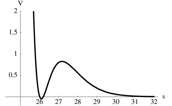
In figure (6) we see that the two solutions in (55) correspond to an AdS minimum and a de Sitter maximum. In fact, the AdS minimum at is supersymmetric. The general solution for given in (52) can also be obtained by methods of section III, imposing the SUSY condition on the corresponding -term by setting it to zero, while introducing the same auxiliary constraint as in (36).
V.2 Two moduli case
While the previous example with one modulus is interesting, it does not capture some very important properties of the vacua which arise when two or more moduli are considered. In particular, in this subsection we will see that the supersymmetric AdS minimum, obtained in the one-dimensional case, actually turns into a saddle point whereas the stable minima are AdS with spontaneously broken supersymmetry. Let us now consider a particularly simple example with two moduli. Here we will choose both moduli to appear on an equal footing in the Kähler potential (1) by choosing
| (57) |
We now have four possible combinations for :
| (58) |
corresponding to the following possible values of :
| (59) |
where only two of the four actually produce independent solutions. The case when has been solved in the previous subsection with , and , given by (50-51) with the moduli taking on the following values for the supersymmetric AdS extremum
| (60) | |||
and the de Sitter extremum
| (61) | |||
As mentioned earlier, the supersymmetric solution can also be obtained by the methods of section III. Now, we also have a new case when . The corresponding two real solutions for and are
| (62) | |||
and
| (63) | |||
where we defined
| (64) |
The moduli are then extremized at the values given by
| (65) | |||
and
| (66) | |||
To completely determine the extrema we again need to substitute the solutions given above into the constraint equation (36) and choose a particular set of values for , , , and to find numerical solutions that result in real positive values for the moduli and . Here we again use the same values as we chose in the previous case given by
| (67) |
For the SUSY extremum we have
| (68) |
The de Sitter extremum is given by
| (69) |
The other two extrema are at the values
| (70) |

It is interesting to note that the supersymmetric extremum in (68) is no longer a stable minimum but instead, a saddle point. The two symmetrically located stable minima seen in figure (7) are non-supersymmetric. Thus we have an explicit illustration of a potential where spontaneous breaking of supersymmetry can be realized. The stable minima appear symmetrically since both moduli were chosen to be on an equal footing in the scalar potential. With a slight deviation where and/or one of the minima will be deeper that the other. It is important to note that at both minima, the volume given by (2) is stabilized at the value which is large enough for the supergravity analysis presented here to be valid.
V.3 Generalization to many moduli
In the previous section we demonstrated the existence of stable vacua with broken SUSY for the special case with two moduli. Here we will extend the analysis to include cases with an arbitrary number of moduli for any value of the parameter . It was demonstrated in section III.2 that the SUSY extremum has an approximate analytical solution given by (29). Therefore, it would be highly desirable to obtain approximate analytical solutions for the other extrema in a similar way. We will start with the observation that for the SUSY extremum (60) obtained for the special case when , both and given by (50) are independent of . On the other hand, if in the leading order parameter is given by (28), from the definitions in (37) it follows that in this case
| (71) |
Thus, if we consider the system (42) in the limit when , we should be able to still obtain the SUSY extremum exactly. In addition, one might also expect that the solutions for the vacua with broken SUSY may also be located near the loci where . With this in mind we will take the limit (71) which results in the following somewhat simplified system of equations for and :
| (72) | |||
Because system (72) is completely decoupled from the constraint (36) and hence the microscopic constants, we can perform a completely general analysis of the vacua valid for arbitrary values of the microscopic constants, at least when the limit (71) is a good approximation. It is straightforward to see that (50) is an exact solution to the above system when . Moreover, unlike the general case when is finite, where the system had three real solutions two of which resulted in positive moduli, system (72) above completely degenerates when yielding only one solution corresponding to the SUSY extremum. On the other hand, for an arbitrary the system has four solutions. One can check that at every point in the range exactly two out of these four solutions are real. The corresponding plots are presented in Figure 8. Before we discuss the plots we would like to introduce some new notation:
| (73) |
where corresponding to the two real solutions. In this notation (44) can be reexpressed as:
| (74) |
The volume of the associative three cycle for these vacua is then:
| (75) |
For future convenience we will also introduce
| (76) |
Constraint (36) is then given by:
| (77) |
which is coupled to
| (78) |
where definitions (37) were used to substitute for and . Both and are completely determined by the system (72), whereas is determined from (77-78). Then solution (74) can be conveniently expressed as
| (79) |
Recall that . Thus the only two possibilities for for any are
| (80) |
As we vary parameter over the range point by point, system (72) always has exactly two real solutions. In Figure 8 we present plots of , and , where as functions of .
 |
 |
Left: Plots of , and corresponding to the first real solution at each . There is a critical value where and becomes positive for .
Right: Plots of , and corresponding to the second real solution at each .
We only need to consider the positive range because of the symmetry (49).
What happens to these solutions when ? We already know from the previous discussion that the system (72) obtained in the limit degenerates for and one obtains the solution that corresponds to the SUSY extremum explicitly. The solutions plotted in Figure 8 were obtained assuming and therefore have an apparent singularity when . Thus they cannot capture either the SUSY or the de Sitter extrema that arise in this special case. To explain what happens to the de Sitter extremum we need to examine the exact solution in (51), in the same limit. Indeed, bearing in mind that is negative, from (51) we have
| (81) |
Here we see immediately that in the limit for the solution above . Therefore we conclude that the de Sitter extremum cannot be obtained from (72) which correlates with the previous observation that for (72) has only one solution - the SUSY extremum. Nevertheless, as we will see in the next subsection the real solutions plotted in Figure 8 are a very good approximation to the exact numerical solutions corresponding to the AdS vacua with spontaneously broken supersymmetry.
Now we would like to classify which of these AdS vacua have all the moduli stabilized at positive values. Indeed if some of the moduli are fixed at negative values we can automatically exclude such vacua from further consideration since the supergravity approximation assumes that all the moduli are positive. Since the volume is always positive by definition, from (79) we see immediately that for all moduli to be stabilized in the positive range, all three quantities , and must have the same sign. In Figure 8 the plots on the right satisfy this requirement for the entire range . On the other hand, the short-dashed curve corresponding to on the left plot is negative when , features a zero at and becomes positive for . Yet, both and remain negative throughout the entire range. Moreover, it is easy to verify that the solution with and , such that is also an exact solution for the general case (42) when is finite. Therefore, all solutions compatible with the SUGRA approximation can be classified as follows:
Given a set of with , there are possible values of , including the negative ones. From the symmetry in (49), only half of those give independent solutions. This narrows the possibilities to positive combinations that fall in the range . For each in the range there exist exactly two solutions describing AdS vacua with broken SUSY with all the moduli fixed at positive values.
For each in the range there exists exactly one solution describing an AdS vacuum with broken SUSY with all the moduli stabilized in the positive range of values. For there are exactly two solutions with all the moduli stabilized in the positive range - de Sitter extremum in (51) and the SUSY AdS extremum in (50). These two solutions are always present for any set of .
V.4 Explicit approximate solutions
In this section we will complete our analysis of the AdS vacua and obtain explicit analytic solutions for the moduli. We will take an approach similar to the one we employed in section III.2 when we obtained an approximate formula (29). Expressing from (78) we obtain
| (82) |
There exists a natural limit when the volume of the associative cycle is large. Just like in the approximate SUSY case in (28), the leading order solution to (82) in this limit is given by
| (83) |
independent of and . Plugging this into (77) and solving for we have in the leading order
| (84) |
where we again assumed the hidden sector gauge groups to be and . Notice that this approximation automatically results in the limit and therefore, , and computed by solving (72) and plotted in Figure 8 are consistent with this approximation. Thus, combining (84) with (79) and (23) we have the following approximate analytic solution for the moduli in the leading order:
| (85) |
To verify the approximation we can check it for the previously considered special case with two moduli when , i.e. the case when . By solving (72) we obtain:
| (86) | |||
Thus, we have the following two solutions for the moduli for the AdS vacua with broken SUSY:
| (87) | |||
and
| (88) | |||
The choice of the constants given in (67) results the following values:
| (89) |
A quick comparison with the exact values in (70) obtained numerically leads us to believe that the approximate analytical solutions presented here are highly accurate. This is especially true when the volume of the associative cycle is large. For the particular choice above the approximate value is:
| (90) |
which is indeed fairly large. To complete the picture, we also would like to include the first subleading order contributions to the approximate solutions presented here. After a straightforward computation we have the following:
| (91) |
and
| (92) |
By combining (92) with (79) and (23) it is easy to obtain the corresponding expressions for the moduli that include the first subleading order correction:
| (93) |
VI Vacua with charged matter in the Hidden Sector
Thus far, we have studied in reasonable detail, the vacuum structure in the cases when the hidden sector has two strongly coupled gauge groups without any charged matter. It is of interest to study how the addition of matter charged under the hidden sector gauge group changes the conclusions. We argue that the addition of charged matter can give rise to Minkowski or metastable de Sitter (dS) vacua due to additional -terms for the hidden sector matter fields. Hence, dS vacua are obtained without adding any anti-branes which explicitly break supersymmetry. This possibility was first studied in Lebedev:2006qq. Moreover, we explain why it is reasonable to expect that for a given choice of -manifold, the dS vacuum obtained is unique.
VI.1 Scalar Potential
Generically we would expect that a hidden sector gauge theory can possess a fairly rich particle spectrum which, like the visible sector, may include chiral matter. For example, an gauge theory apart from the “pure glue” may also include massless quark states and transforming in and of . When embedded into theory the effective superpotential due to gaugino condensation for such a hidden sector with () quark flavors has the following form Seiberg:1994bz:
| (94) |
We can introduce an effective meson field to replace the quark bilinear
| (95) |
and for notational brevity we define
| (96) |
Here we will consider the case when the hidden sector gauge groups are and with flavors of the quarks () transforming as () under and as singlets under . In this case, when , the effective nonperturbative superpotential has the following form:
| (97) |
One serious drawback of considering hidden sector matter is that we cannot explicitly calculate the moduli dependence of the matter Kähler potential. Therefore we will have to make some (albeit reasonable) assumptions, unlike the cases studied in the previous sections. In what follows we will assume that we work in a particular region of the moduli space where the Kähler metric for the matter fields in the hidden sector is a very slowly varying function of the moduli, essentially a constant. This assumption is based on the fact that the chiral fermions are localized at point-like conical singularities so that the bulk moduli should have very little effect on the local physics. In general, a singularity supporting a chiral fermion has no local moduli, since there are no flat directions constructed from a single chiral matter representation. Our assumption is further justified by the theory lift of some calculable Type IIA matter metrics as described in the appendix. It is an interesting and extremely important problem to properly derive the matter Kähler potential in theory and test our assumptions.
Thus we will consider the case when the hidden sector chiral fermions have “modular weight zero” and assume a canonically normalized Kähler potential. The scalar potential is invariant under and along the -flat direction. For the sake of simplicity, we will first study the case , but later it will be shown that all the results also hold true for . The meson field along the -flat direction is such that the corresponding Kähler potential for is canonical. The total Kähler potential, i.e. moduli plus matter thus takes the form:
| (98) |
The moduli -terms are then given by
| (99) | |||||
In addition, an -term due to the meson field is also generated
| (100) |
The supergravity scalar potential is then given by:
| (101) | |||||
Minimizing this potential with respect to the axions and we obtain the following condition:
| (102) |
The potential has local minima with respect to the moduli when
| (103) |
In this case (101) reduces to
| (104) | |||||
VI.2 Supersymmetric extrema
Here we consider a case when the scalar potential (104) possess SUSY extrema and find approximate solutions for the moduli and the meson field vevs. Taking into account (103) and setting the moduli -terms (99) to zero we obtain
| (105) |
together with the constraint
| (106) |
At the same time, setting the matter -term (100) to zero results in the following condition:
| (107) |
Expressing from (105) and substituting it into (107) we obtain the following solution for the meson vev at the SUSY extremum:
| (108) |
Recall that in our analysis we are considering the case when , which implies that parameter defined in (96) is negative. Thus, since the left hand side of (108) is positive, for the SUSY solution to exist, it is necessary to satisfy
| (109) |
Recall that for the moduli to be positive, the constants have to satisfy certain conditions resulting in two possible branches (III.2). Therefore, condition (109) implies that the SUSY AdS extremum exists only for branch a) in (III.2). In the limit, when is large, the approximate solution is given by:
| (110) | |||
where we also assumed that , such that . For the case with two moduli where and the choice
| (111) |
the numerical solution for the SUSY extremum obtained by minimizing the scalar potential (104) gives
| (112) |
whereas the approximate analytic solution obtained in (110) yields
| (113) |
This vacuum is very similar to the SUSY AdS extremum obtained previously for the potential arising from the “pure glue” Super Yang-Mills (SYM) hidden sector gauge theory. Thus, we will not discuss it any further and instead move to the more interesting case, for which condition (109) is not satisfied.
VI.3 Metastable de Sitter (dS) minima
Below we will use the same approach and notation we used in section V, to describe AdS vacua with broken SUSY. Again, for brevity we denote
| (114) |
Extremizing (104) with respect to the moduli and dividing by we obtain the following system of coupled equations
| (115) | |||||
plus the constraint (106). Next, we extremize (104) with respect to and divide it by to obtain:
| (116) | |||
To solve the system of cubic equations (115), we introduce a quadratic constraint
| (117) |
such that (115) turns into a system of coupled quadratic equations:
| (118) |
Again, the standard solution of a quadratic equation dictates that the solutions for of (118) have the form
| (119) |
We have now reduced the task of determining for each to finding only two quantities - and . By substituting (119) into equations (116-118) and using (2), we obtain a system of three coupled equations
| (120) | |||
plus the constraint (106). Note that each solution is again labelled by parameter so that (119) becomes
| (121) |
Let us consider the case when . In this case, the solution is given by
| (122) |
and (120) is reduced to
| (123) | |||
In the notation introduced in (114), the SUSY condition (107) can be written as
| (124) |
It is then straightforward to check that in the SUSY case, the system (123) yields
| (125) |
as expected. We will now consider branch b) in (III.2) for which (124) is not satisfied. Moreover, in order to obtain analytical solutions for the moduli and the meson vev we will again consider the large three cycle volume approximation. Recall that in this case we take and limit to obtain the following reduced system of equations when for and :
| (126) | |||
Note that in (126), we have dropped the third equation since for we only need to know and the third equation in (123) determines in terms of . We also kept the first subleading term in the second equation. Note that the term in the second line of the first equation proportional to appears to blow up as . However, from the second equation one can see that the combination is proportional to which makes the corresponding term finite. By keeping the subleading term in the second equation, we can express
| (127) |
from the second equation to substitute into the first equation to obtain in the leading order
| (128) |
Since we are now considering branch b) in (III.2), the second factor in (128) is automatically non-zero. Therefore, the first factor in (128) must be zero. Thus, after substituting
| (129) |
obtained from (127), we have the following equation for
| (130) |
Also, since in the leading order , using the definitions in (114) we can express from (122) in the limit when is large, including the first subleading term
| (131) |
By combining (106) with the leading term in (131) and taking into account that we again obtain
| (132) |
Thus, from (131) we have
| (133) |
Finally, using (133) along with the definitions of , and in (114) in terms of we can solve for from (130) and assuming that , in the limit when is large we obtain
| (134) |
We notice immediately that since is real and positive it is necessary that
| (135) |
We will show shortly that the extremum we found above corresponds to a metastable minimum. Also, for a simple case with two moduli, via an explicit numerical check we have confirmed that if the local minimum is completely destabilized yielding a runaway potential. Also note that for (134) to be accurate, it is not only which has to be large but also the product has to stay large to keep the subleading terms suppressed. To check the accuracy of the solution we again consider a manifold with two moduli where the values of the microscopic constants are:
| (136) |
The exact values obtained numerically are:
| (137) |
The approximate equations above yield the following values:
| (138) |
Note the high accuracy of the leading order approximation for the moduli .
It is now straightforward to compute the vacuum energy using the approximate solution obtained above. First, we compute
| (139) |
and
| (140) |
Using (129), (139) and (140) we obtain the following expression for the potential at the extremum with respect to the moduli as a function of
| (141) |
where the terms linear in cancelled and the quadratic terms were dropped. A quick look at the structure of the potential (141) as a function of , where , is enough to see that there is a single extremum with respect to which is indeed, a minimum. The polynomial in the square brackets is quadratic with respect to . Moreover, the coefficient of the monomial is equal to unity and therefore is always positive. This implies that for the minimum of such a biquadratic polynomial to be positive, it is necessary for the corresponding discriminant to be negative, which results in the following condition:
| (142) |
Again, since in the leading order , using the definitions in (132), we can express from (122) in terms of to get
| (143) |
We then substitute from (132) into (143) and use it together with we obtain from (142) the following condition
| (144) |
The above equation is the leading order requirement for the energy density at the minimum to be positive. It is also clear that the minimum is metastable, as in the decompactification limit (), the scalar potential vanishes from above, leading to an absolute Minkowski minimum. Figure 9 shows the scalar potential for a manifold with two moduli along the slice with the meson field equal to its value at the minimum of the potential (134). The microscopic constants are the same as in (136).

VI.4 The uniqueness of the dS vacuum
In the previous subsection we found a particular solution of the system in (120) corresponding to . Here we would like to investigate if solutions for are possible when the vacuum for is de Sitter. Just like for the pure Super Yang-Mills (SYM) case, we can recast (121) as
| (145) |
where the volume of the associative three cycle is again
| (146) |
and we have introduced
| (147) |
Just like we did in equation (82) for the pure SYM case, we can also express as
| (148) |
If we again consider the large associative cycle volume limit and take and , the second and third equations in (120) in the leading order reduce to
| (149) | |||
Note that the only difference between (72) and (149) is the presence of the term
| (150) |
which couples the system (149) to the first equation in (120) which determines . Instead of solving the full system to determine , and and analyzing the solutions we choose a quicker strategy for our further analysis. Namely, we can solve the system of two equations in (149) and regard as a continuous deformation parameter. One may object to this proposition because and therefore are not independent of parameter . However, in the limit when is large, we notice from (148) that in the leading order, is indeed independent of .
Recall that in the pure SYM case the system (72) corresponding to the case when has two real solutions for all . Thus, one may expect that as we continuously dial , the system may still yield real solutions for . Let us first determine the range of possible values of parameter . A quick calculation yields that the combination in (150) is the smallest with respect to when . In this case
| (151) |
Now, recall from the previous subsection that for the solution corresponding to to have a positive vacuum energy, condition (142) must hold. Since and are independent of in the leading order, condition (142) implies that
| (152) |
Again, since the volume is always positive, from (145) we see that for all moduli to be stabilized in the positive range, all three quantities , and must have the same sign. For , the system (149) has two real solutions when .
 |
 |
However, from the left plot in Figure 10 corresponding to the minimum value we see that neither of the two solutions satisfy the above requirement since both short-dashed curves corresponding to for the two solutions are always positive for the entire range , whereas both and remain negative. Therefore for and there are no solutions for which all the moduli are stabilized at positive values. Moreover, as parameter is further increased, the range of possible values of for which the system has two real solutions gets smaller and more importantly, the values of remain positive and only increase while both and remain negative, which can be seen from the right plot in Figure 10, where . This trend continues as we increase .
Thus, we can make the following general claim: If the solution for has a positive vacuum energy, condition (152) must hold. When this condition is satisfied the system (149) has no solutions in the range for which all the moduli are stabilized at positive values. Therefore, if the vacuum found for is de Sitter it is the only possible vacuum where all the moduli are stabilized at positive values. Although the above analysis was done in the limit when is large, we have run a number of explicit numerical checks for a manifold with two moduli and various values of the constants confirming the above claim. In addition, although we have not proved it, it seems plausible from many numerical checks we carried out that it is also not possible to have a metastable dS minimum for values of different from unity, even if the dS condition on the vacuum is not imposed.
Finally, it should be noted that the situation with a “unique” dS vacuum is in sharp contrast to that when one obtains anti-de Sitter vacua, where there are between and solutions for moduli depending on the value of (see section V). Let us explain this in a bit more detail. Since the dS solution found for is located right in the vicinity of the ‘‘would be AdS SUSY extremum’’33 3 This can be seen by comparing the leading order expression for the moduli vevs in the dS case (132) with the corresponding formula for the SUSY AdS extremum (31). where the moduli -terms are nearly zero, it is the large contribution from the matter -term (140) which cancels the term in the scalar potential resulting in a positive vacuum energy. Recall that in the leading order all the AdS vacua with the moduli vevs are located within the hyperplane 44 4 c=1,2 labels the two real solutions of the system (72).
| (153) |
The matter -term contribution to the scalar potential evaluated at the same but arbitrary is therefore also constant along the hyperplane (153). Thus, while the matter -term contribution stays constant, as we move along the hyperplane (153) away from the dS minimum, where the moduli -terms are the smallest, the moduli -term contributions can only get larger so that the scalar potential becomes even more positive. This implies that the AdS minima with broken SUSY found in Section V completely disappear, as the AdS SUSY extremum becomes a dS minimum.
VII Relevant Scales
We have demonstrated above that in fluxless theory vacua, strong gauge dynamics can generate a potential which stabilizes all the moduli. Since the entire potential is generated by this dynamics, and the strong coupling scale is below the Planck scale, we also have a hierarchy of scales. In this section we calculate some of the basic scales in detail. In particular, the gravitino mass, which typically controls the scale of supersymmetry breaking is calculated. By uniformly scanning over the constants with order one, we demonstrate in VII.3 that a reasonable fraction of choices of constants have a TeV scale gravitino mass. We do not know if the space of -manifolds uniformly scans the or not, and more importantly, the scale of variation of the ’s in the space of manifolds is not clear. The variation of the ’s is the most important issue here, since one can certainly vary and over an order of magnitude. We begin with a discussion of the basic scales in the problem. We will begin with the AdS vacua, then go on to discuss the de Sitter case. In particular, in the dS case, requiring a small vacuum energy seems to lead to superpartners at around the TeV scale. It will also be shown that including more than one flavor of quarks in the hidden sector or including matter in both hidden sectors does not change this result. The section will end with an estimation of the height of the potential barrier in these vacua.
VII.1 Scales: AdS Vacua
As an example, we consider one of the non-SUSY minima in our toy model given by (70) and compute some of the quantities relevant for phenomenology. Namely, the vacuum energy
| (154) |
the gravitino mass
| (155) |
the 11-dimensional Planck scale
| (156) |
the scale of gaugino condensation in the hidden sectors
| (157) | |||||
| (158) |
where GeV is the reduced four-dimensional Planck mass.
VII.2 Gravitino mass
By definition, the gravitino mass is given by:
| (159) |
For the particular theory vacua with Kähler potential given by (1) and the non-perturbative superpotential as in (5) with and hidden sector gauge groups we have:
| (160) |
where the relative minus sign inside the superpotential is due to the axions. Before we get to the gravitino mass we first compute the volume of the compactified manifold for the AdS vacua with broken SUSY. By plugging the approximate leading order solution for the moduli (85) into the definition (2) of we obtain:
| (161) |
Recalling the definition (75) of and using (84) together with (161) to plug into (160) the gravitino mass for these vacua in the leading order approximation is given by:
| (162) |
For the special case with two moduli when , considered in the previous sections we obtain the following:
| (163) | |||||
For the choice of constants as in (67) the leading order approximation (163) yields:
| (164) |
whereas the exact value computed numerically for the same choice of constants is:
| (165) |
Again, we see a good agreement between the leading order approximation and the exact values.
VII.3 Scanning the Gravitino mass
In previous sections we found explicit solutions describing vacua with spontaneously broken supersymmetry. Moreover, we also demonstrated that for a particular set of the constants these solutions can result in . It would be extremely interesting and worthwhile to estimate (even roughly) the fraction of all possible solutions which exhibit spontaneously broken SUSY at the scales of - TeV. We would first like to do this for generic AdS/dS vacua with a large magnitude of the cosmological constant (). The analysis for the AdS vacua is given below but as we will see, the results obtained for the fraction of vacua are quite similar for the dS case as well. In subsection VII.4, we impose the requirement of a small cosmological constant as a constraint and try to understand its repercussions for the gravitino mass.
We do not yet know the range that the constants take in the space of all manifolds. Nevertheless, we do have a rough idea about some of them. For example, we expect that the quantity given by the ratio
| (166) |
which appears in several equations, does deviate from unity. One reason for this may be due the threshold corrections Friedmann:2002ty which in turn depend on the properties of a particular -holonomy manifold. For concreteness, we take an upper bound . Also, based on the duality with the Heterotic String we can get some idea on the possible range of integers and corresponding to the dual coxeter numbers of the hidden sector gauge groups. Namely, since for both and gauge groups appearing in the Heterotic String theories the dual coxeter numbers are , we can tentatively assume that both and can be at least as large as . Of course, we do not rule out any values higher than but in this section we will assume an upper bound .
We now turn our attention to equation (162) which will be used to estimate the gravitino mass scale. It is clear from the structure of the formula that is extremely sensitive to , as well as the ratio , given by (166). On the other hand it is less sensitive to the other constants appearing in the equation such as , and the ratios . This is because the powers for each term under the product get much less than one as the number of moduli increases because of the constraint on in (2). This will smooth any differences between the contributions coming from the individual factors inside the product. Since for ( is defined in (44)), the ratios vary only in the range -, for our purposes it will be sufficient to simply consider (162) for the case when corresponding to the SUSY extremum so that for all . This is certainly good enough for the order of magnitude estimates we are interested in. It also seems reasonable to assume that the integers are all of . Yet, even if some are unnaturally large, their individual contributions are generically washed out since they are raised to the powers that are much less than one. Thus, for simplicity we will take for all . Finally, from field theory computations Finnell:1995dr, (in a particular RG scheme) up to threshold corrections. We therefore take for simplicity, allowing to vary.
Thus, the gravitino mass in our analysis is given by
| (167) |
Finally, with regard to the constants which are a subject to the constraint
| (168) |
we will narrow our analysis to two opposite cases. For the first case we make the following choice
| (169) |
such that one modulus is generically large and all the other moduli are much smaller. This is a highly anisotropic -manifold. The second case is
| (170) |
with all the moduli being on an equal footing. Therefore, by considering these opposite cases we expect that most other possible sets of will give similar results that are somewhere in between. For each set of above, equation (167) gives
| (171) |
| (172) |
For a typical compactification we expect , therefore the variation of due to an change in the number of moduli for the first case is whereas in the second case it can be as large as . Thus, if we choose , we expect that our order of magnitude analysis will be fairly robust for case . For case , however, we will perform the same analysis for and to see how different the results will be. Before we proceed further we need to impose a restriction on the possible solutions to remain within the SUGRA framework. Using (161), condition that must remain greater than one for the two cases under consideration translates into the following two conditions:
| (173) |
| (174) |
Then, as long as conditions (173-174) hold, volume of the associative cycle is greater than one is satisfied automatically - a necessary condition for the validity of supergravity. This is obvious from comparing the right hand side of (84) with each condition above. From (173-174) we can find a critical value of for both cases at which :
| (175) |
| (176) |
By substituting (175-176) into (171-172) we can find the corresponding upper limits on as functions of and , below which our solutions are going to be consistent with the SUGRA approximation.
In Figure 11 we present plots of for both cases as a function of in the range where for different values of .
 |
 |
 |
 |
On all the plots the light grey area represents possible values of consistent with the supergravity framework. For the sake of completeness we have also included the formal plot of corresponding to represented by the dashed curve. ¿From the plots it is clear that as the difference is increased from to - top and from to - bottom, both the light grey area representing all possible values of consistent with the SUGRA approximation and the dark area corresponding to get significantly smaller. If we further increase , the light grey region shrinks even more for case , and does not exist for case , while the dark region completely disappears in both cases. Therefore, for case the plots on the bottom of Figure 11 are the only possibilities where solutions for and consistent with the SUGRA approximation are possible, implying un upper bound . It turns out that for case the upper bound on where such solutions are possible is much higher .
Assuming that all values of the constants such as , and are equally likely to occur in the ranges chosen above we can perform a crude estimate of the number of solutions with relative to the total number of possible solutions consistent with the SUGRA approximation. In doing so we will use the following approach. For each value of in the range we compute the area of the grey region for each plot and then add all of them to find the total volume corresponding to all possible values of consistent with the supergravity approximation.
| (177) |
Likewise, we add all the dark areas for each plot to find the volume corresponding to the region where
| (178) |
where is un upper bound before the dark region completely disappears. From the previous discussion, for case : ; for case : . Then, the fraction of the volume where is given by the ratio
| (179) |
Numerical computations yield the following values for the two cases when :
| (180) |
| (181) |
Because of the significant difference in the dependence of on the number of moduli in (175) versus (176), the number of solutions consistent with the SUGRA approximation is cut down dramatically in case compared to case . This also occurs because of the different dependence of in (171) and (172) on . Namely, for , the values of for case in (172) are greater than those for case . Furthermore, for the same reasons, it turns out that if we keep increasing the number of moduli , for case there is un upper bound for the solutions with compatible with the SUGRA approximation to exist at all. Of course, this upper bound can be higher if we allow to be greater than .
By performing the same analysis for we get the following estimates
| (182) |
| (183) |
As expected, decreasing the number of moduli by a half has produced little effect on while decreasing by a few present. These numbers coming from our somewhat crude analysis already demonstrate that a comparatively large fraction of vacua in theory generate the desired hierarchy between the Planck and the electroweak scale physics. Also, one can easily check that all the solutions consistent with the SUGRA framework for which for any number of moduli satisfy the following bound on the eleven dimensional scale
| (184) |
which makes them compatible with the standard unification at GeV. This is also a nice feature. Of course, apart from determining the upper and lower bounds on the constants, it would be desirable to know their distribution for all possible manifolds of holonomy. In this case instead of using the flat statistical measure as we did here, each solution would be assigned a certain weight making the sampling analysis more accurate. However, this is an extremely challenging task which goes beyond the scope of this work.
The simple analysis presented in this section clearly points to a very restrictive nature of the solutions. Namely, the requirement of consistency with the supergravity regime results in very strict bounds on the properties of the compactification manifold. Further requirements coming from the SUSY breaking scale to be in the range required for supersymmetry to solve the hierarchy problem narrows down the class of possible holonomy manifolds even more. It would be extremely interesting to know to what extent these results extend into the small volume, ”stringy” regime, about which we have nothing to say here.
VII.3.1 Results for dS Vacua
We will now show that the results obtained in the previous subsection also hold true for dS vacua with Kähler potential given by (98) and the non-perturbative superpotential as in (97) with and hidden sector gauge groups. For this case, we have :
| (185) |
where the relative minus sign inside the superpotential is due to the axions and . Before we get to the gravitino mass we first compute the volume of the compactified manifold for the metastable dS vacuum with broken SUSY. By substituting the approximate leading order solution for the moduli (132) into the definition (2) of we obtain:
| (186) |
Recalling the definition of Im() in terms of and using the solution for (eqn.(132)) together with (186), the gravitino mass for the dS vacuum in the leading order approximation is given by:
| (187) |
where is given by (134). Since from section VI and , we see that the expression for the gravitino mass for dS vacua is almost the same as that for the AdS vacua (eqn. 167) provided we replace in (167) by in (187) and in (167) by in (187).
For the de Sitter vacua, we use a less restrictive upper bound . For a manifold with moduli we obtain:
| (188) |
| (189) |
In Figure 12 we present plots of for both cases as a function of in the range where for different values of .
 |
 |
 |
 |
VII.4 Small Cosmological Constant implies Low-scale Supersymmetry in dS Vacua
In this subsection we will study the distribution of SUSY breaking scales in the de Sitter vacua which as we showed earlier, can arise when the hidden sector has chiral matter. In particular we will see that the requirement of a small cosmological constant leads to a scale of SUSY breaking of TeV.
In section VI, we saw that the minimum obtained is de Sitter if the discriminant of the quadratic polynomial with respect to in eqn. (141) is negative, while it is anti-de Sitter if the discriminant in (141) is positive. For the magnitude of the vacuum energy in both cases can be estimated to be
| (190) |
On the other hand, if the discriminant in (141) vanishes, one obtains a vanishing cosmological constant (to leading order in the approximation). At present it is not known if there is a physical principle which imposes this condition. However, one can still use it as an observational constraint since the observed value of the cosmological constant is known to be extremely small. For instance, it could happen that the space of manifolds scans the constants finely enough such that there exist vacua for which the vacuum energy is acceptably low. In particular, the constants which are determined by the threshold corrections have been shown to depend on integers55 5 This is because the threshold corrections can be related to certain topological invariants of the associative three-cycle. Friedmann:2002ty. In this work, we will assume that to be the case. A detailed computation to show this in a convincing manner is currently being attempted and will be reported in the future. It should also be kept in mind that a different mechanism for solving the cosmological constant, completely decoupled with particle physics, could exist. Such a mechanism, if present, would not affect any predictions for low energy particle physics.
By setting the left hand side in (144) to zero, we can then express
| (191) |
Of course, since the above constraint was obtained in the leading order, the vacuum energy is only zero in the leading order in our analytic expansion. The subleading contributions we neglected in (225) although smaller than the leading contributions, are still much larger than the observed value of the cosmological constant. However, one can in principle take into account all the subleading corrections and tune the ratio inside the logarithm to set the vacuum energy to a very small value compatible with the observations. As will be seen later, since the expression in the R.H.S. of (191) turns out to be large, the subleading corrections which affect the value of the cosmological constant will have little effect on the phenomenological quantities calculated by imposing the constraint to leading order.
We would now like to analyze in detail the phenomenological implications of the solutions obtained by imposing (191) as a constraint. The most important phenomenological quantity in this regard is the gravitino mass as it sets the scale of all soft supersymmetry breaking parameters. We focus on the gravitino mass in this section. The soft supersymmetry breaking parameters will be discussed in section VIII.
VII.4.1 Gravitino mass with a small positive cosmological constant
By substituting the constraint (191) into the gravitino mass formula (187), we obtain:
| (192) |
where the meson vev is now given by:
| (193) |
In this case, the moduli vevs are given by
| (194) |
From (192), one notes that the gravitino mass (when the cosmological constant is made tiny) is completely determined by the dual coxeter numbers of the hidden sector gauge groups , the rational numbers (see (2)) characterizing the volume of the manifold and the integers .66 6 From field theory computations Finnell:1995dr, and (in a particular RG scheme), up to threshold corrections. We can therefore express , as and , where coefficients and depend only on the threshold corrections and are constant with respect to the moduli Friedmann:2002ty. In this case, the quantity is fixed by imposing (191).
The rationals are subject to the constraint . It is reasonable to consider a “democratic” choice for , for all and also to take for simplicity all the integers . The integers will generically be of ; even if some of the are unnaturally large, their individual contributions will be typically washed out as they are raised to powers that are much less than unity (see (187) and the expression for for the democratic choice). In this case, after setting , the gravitino mass formula is given by
| (195) |
and the moduli vevs are
| (196) |
From (195), the gravitino mass depends on just four constants - , , and (the total number of moduli), determined by the topology of the manifold. It should be kept in mind that for the solution to exist, it is necessary that (see (135)). For the smallest possible value , the expression for simplifies even further
| (197) |
together with
Note that the dependence on and in (197) is due solely to the volume dependence on those parameters. The expression for the gravitino mass has a more transparent form if we don’t substitute the expression for the volume (186) into (185). For we obtain
| (198) |
where the detailed dependence on , , and the number of moduli is completely encoded inside the seven-dimensional volume which appears to be the more relevant physical quantity. Furthermore, in the supergravity approximation the volume , which translates into an upper bound on the gravitino mass when
| (199) |
VII.4.2 The Gravitino mass Distribution and its consequences
The gravitino mass (195) depends on three integers: the two gauge group dual coxeter numbers , and the number of moduli .77 7 We can set for the order of magnitude estimates we are doing here. This will give us an idea about the distribution of the gravitino mass (which sets the superpartner masses) obtained after imposing the constraint (191) that the vacuum energy is acceptable. Asides from only considering the vacua within the supergravity approximation (ie ) we expect an upper bound on the dual coxeter numbers of the hidden sector gauge groups and . Based on duality with the heterotic string, it seems reasonable to assume that they can be at least as large as 30 - the dual coxeter number of . Of course, values of larger than 30 cannot be ruled out, and here we assume an upper bound . Notice that from the constraint in (191), the ratio can get exponentially large when and the values of are small. Here we are going to completely relax the requirement on the upper bound of the ratio because as we will see, for generic manifolds with a large numer of moduli, has to be large for the supergravity approximation to hold. The distribution can be constructed as follows. The three integers: , and are varied subject to (135) and the supergravity constraint . For each point in the resulting two dimensional subspace, can be computed and rounded off to the closest integer value. One can then count how many times each integer value is encountered in the entire scan and plot the corresponding distribution.
 |

 |
In the first three scans scan we cover a broad range of values by choosing . Taking into account the SUGRA constraint (), we have the following ranges of integers for the first scan:
| (200) |
In the second scan we have excluded the small N region and considered only the manifolds with . Thus we have the following ranges of constants for the second scan:
| (201) |
In the third scan we have only considered manifolds with . Thus we have the following ranges of integers for the second scan:
| (202) |
The first two distributions in Figure 13 clearly have several prominent peaks. Amazingly, in all three plots one of the peaks landed right in the range! The high scale peaks on the left plot appear to be around and the GUT scales. However, for the middle plot the GUT scale peak almost disappears. Recall that the middle plot corresponds to scan two in (201) where we excluded all the manifolds for which the number of moduli is less than . Therefore, the high scale peaks are largely dominated by contributions from the manifolds with a small number of moduli . As seen from the right plot, when manifolds with are excluded from the scan, the peak at the scale has all but disappeared, whereas the peak at remains virtually unchanged.
In Figure 14 we included three more scans for which the upper bound on was reduced to . The fourth scan has the following ranges:
| (203) |
In the fifth scan we again excluded the small N region an considered only the manifolds with and considered :
| (204) |
In the sixth scan we considered only the manifolds with and :
| (205) |
 |

 |
Again, in Figure 14 we notice that the peak narrows around , as we exclude manifolds with small number of moduli. As the same time, the peaks at the high scale completely disappear for manifolds with . Finally, in Figure 15 we chose the smallest possible value
 |

 |
and scanned integers and in the following ranges:
| (206) | |||
In all three plots in Figure 15 we see the same peak at , which narrows around as is decreased.
Therefore, from the above distributions we conclude that the peak corresponding to is entirely due to the smallest possible value . This can be explained if we examine the gravitino mass formula in (197). In particular the constant factor is most crucial in lowering the gravitino mass to the TeV scale. It is easy to trace the origin of this factor to the constraint (191), imposed by the requirement to have a zero cosmological constant (to leading order). When (191) is used along with the requirement we simply get
| (207) |
When this is substituted into the gravitino mass (187), the corresponding suppression factor turns into the constant
| (208) |
Physically, this suppression factor corresponds to the hidden sector gaugino condensation scale (cubed). Recall that for an hidden sector gauge group, the scale of gaugino condensation is given by
| (209) |
The moduli vevs in (194) completely determine the gauge kinetic function. Taking we obtain
| (210) |
Substituting (210) into (209) we obtain the following scale of gaugino condensation
| (211) |
It is important to note that the expression in the R.H.S. of (191) is quite large (, when ) in the leading order, and the quantity () which is fixed by imposing the vacuum energy constraint is inside a logarithm. Therefore, even when one incorporates all the higher order corrections and tunes the ratio inside the logarithm to set the cosmological constant equal to the observed value, the constant on the R.H.S. (=84), crucial in obtaining the scale peak, is hardly affected.
The dominance of the range also becomes clear from Figure 16, where as a function of for is plotted for a manifold with moduli - short-dashed curve, and a manifold with moduli - long-dashed curve.
 |
Indeed, even when we do not impose the SUGRA constraint, from the above plot we can see that the range is covered by a large swath of the vacuum space and it is not so surprising that the corresponding distribution peaks at that scale. This essentially follows from the formula for the gravitino mass in (197).
An important point which should be emphasized is that for , the gravitino mass dependence on and appears only through the volume , as can be seen from (198). Thus, the distribution in Figure 15 directly correlates with the corresponding distribution of the stabilized volume of the seven-dimensional manifold as a function of and . Therefore, it is the dominance of the vacua with a relatively small volume, which results in the peak at .
Also note that in the above analysis we simply set the constant coefficient due to the threshold corrections to unity. It would be interesting to get a handle on this quantity and include its variation into the gravitino mass distribution study.
One could argue that even though gives a peak for the gravitino mass distribution at around scale, it seems plausible from a theoretical point of view to have many examples of gauge singularities in manifolds such that . However, by imposing the supergravity constraint that all moduli are larger than unity (which is the regime in which the entire analysis is valid), one sees that having drastically reduces the upper bound on compared to that for (see eqn(194)). Therefore, the peaks in the gravitino mass distribution obtained for in Figures 13 and 14 come from vacua with a small number of moduli as well as , compatible with the analysis in the supergravity regime. Since it is presumably true that the number of manifolds with the required gauge singularities which have a large number of moduli is much larger than those with a small number of moduli, it seems reasonable to expect that the peak of the gravitino mass distribution obtained at around scale is quite robust and is representative of the most generic class of manifolds with the appropriate gauge singularities. Notice also that in the case of manifolds with a large number of moduli , because of the constraint from the supergravity approximation, the actual minimal value of in the scans (202) and (205) is quite large, i.e. . Hence, if , from (191) the value of the ratio when is bounded from above
| (212) |
On the other hand, for less generic manifolds with a small number of moduli the supergravity constraint allows to be small. In this case in order to satisfy (191), has to be exponentially large. Whether this is possible remains to be seen. However, because for the more generic case when the upper bound in (212) is quite reasonable, our analysis remains robust.
One could also contrast the results obtained above with those obtained for the Type IIB flux vacua. In Type IIB flux vacua, one has to independently tune both the gravitino mass to a TeV scale (if one requires low scale supersymmetry to solve the hierarchy problem) as well as the cosmological constant to its observed value. This is quite different to what we are finding here. Finally, we should emphasize that imposing the supergravity approximation was crucial in obtaining low scale SUSY breaking. Plausibly, the vacua which exist in the theoretic, small volume regime will have a much higher SUSY breaking scale. However, such vacua presumably also have the incorrect electroweak scale (either zero or ).
VII.5 Including more than one flavor of quarks in the hidden sector
In the previous analysis we assumed a single flavor for the quarks in the hidden sector, i.e . In order to check that the way we obtain a dS metastable minimum is robust and not dependent on a particular choice of chiral hidden sector matter spectrum, we would like to extend our analysis to include more than one flavor (but still with ) so that the meson fields are given by:
| (213) |
where . In the absence of a perturbative superpotential (which is guaranteed in the absence of fluxes), one has along the -flat direction:
Thus, the determinant appearing in (94) becomes
| (219) |
The nonperturbative superpotential and the Kähler potential are then given by
| (220) | |||
where we again denoted , , and . After minimizing with respect to the axions, the scalar potential is given by
| (221) | |||||
Instead of presenting a full analysis of this more general case we would simply like to check that we have a metastable dS vacuum, and that the main feature of the dS vacuum, namely the emergence of the TeV scale when the tree-level cosmological constant is set to zero, survives when . For this purpose we need to compute the scalar potential at the minimum with respect to the moduli as a function of the meson fields .
The generalization of the equations minimizing the scalar potential is fairly straightforward. In particular, in the limit when the size of the associative cycle is large, for the generalization of the second equation in (126), which determines takes on the following form
where we again defined , , and . Thus, in the large three-cycle limit we again have so that and the leading order solution for is again given by
| (222) |
In this case the moduli are stabilized at the same values given by (132). Since both the superpotential and the Kähler potential are completely symmetric with respect to the meson fields, it seems reasonable to expect that there is a vacuum where all are stabilized at the same value, i.e. for all . Using the solution for the moduli vevs (132) and the above assumption we obtain the following expression for the potential at the extremum with respect to the moduli as a function of
| (223) |
By setting the discriminant of the biquadratic polynomial in the square brackets to zero we again obtain the leading order condition on the tree-level cosmological constant to vanish:
| (224) |
Since the solutions for the moduli in the dS case correspond to branch b) where and , zero vacuum energy condition (224) can be satisfied only when
| (225) |
Therefore, a vanishing tree-level cosmological constant in the leading order results in the following set of conditions:
| (226) |
Recall that the key to obtaining the TeV scale gravitino mass was the exponential suppression factor when , related to the scale of gaugino condensation. In the present case, up a factor of order one, we have
| (227) |
Consider a few examples where . From (226) we have the following set
| (228) | |||
Remarkably, in all but one cases listed above we obtain the same suppression factor which was the reason for the peak at ! Note that the only example which did not fall into this range was the third case for which the condition on the cosmological constant to vanish was , which is too unrealistic anyway, as it requires either extremely large dual coxeter numbers for the gauge groups or an exponentially large ratio inside the logarithm. On a similar note, as can be seen from the third entry in each line in (228), increasing the number of flavors even further would again require either or an extremely large ratio , which appears inside the logarithm. Therefore, limiting our analysis to the cases with seems quite reasonable.
Recall that for the TeV scale appeared for the minimum value whereas the vacua corresponding to the higher values of generally failed to satisfy the SUGRA constraint for more generic manifolds with a large number of moduli. For this reason, considering larger values of for the examples listed above is probably unnecessary. Hence, for more than one flavor of quarks, we only need to take
| (229) |
Thus, given that the assumptions we made in the beginning of this subsection are reasonable, it appears that the connection of the TeV scale SUSY breaking to the requirement that the tree-level vacuum energy is very small is a fairly robust feature of these vacua, independent of the number of flavors.
VII.6 Including matter in both hidden sectors
In the previous analysis we tried to be minimalistic and included chiral matter in only one of the hidden sectors. Due to this asymmetry, we obtained two types of solutions - a supersymmetric AdS extremum when corresponding to branch a) and a dS minimum when (when condition (144 holds), corresponding to branch b). Using this result it is then fairly straightforward to figure out what happens when both hidden sectors produce F-terms due to chiral matter. For the sake of simplicity, we will again consider the case when in both hidden sectors. In this case, the Kähler potential is given by
| (230) |
After minimizing with respect to the axions, the non-perturbative superpotential (up to a phase) is given by
| (231) |
where and . We will now check to see if it is still possible to obtain SUSY extrema when both hidden sectors have chiral matter. Setting the moduli -terms to zero we obtain
| (232) |
where . At the same time, setting the matter -terms to zero results in the following conditions:
| (233) |
| (234) |
Expressing from (232) and substituting it into (233-234) and using the definitions for and , we obtain the following expressions for the meson field vevs:
| (235) | |||
| (236) |
Since as well as both and are positive definite, we have the following two possibilities:
| (237) | |||
Thus, when both hidden sectors have chiral matter, supersymmetric extrema are absent. Instead, when condition (144) holds (for branch a) we simply swap and , and in (144)), for each branch we obtain a dS vacuum where only one of the matter -terms is non-zero. Keep in mind that although in the above analysis we used condition (232) obtained by setting the moduli -terms to zero, even in the dS case when the moduli -terms are non-zero, one of the two mesons will be stabilized at a value such that the corresponding matter -term is zero. The zero -term has no effect on the analysis of the dS solution and apart from replacing with defined above, the same solution obtained previously for the dS vacuum applies. In this case, the only difference will be in the meson field vevs:
| (238) | |||
Therefore, the dS solution obtained for the minimal case when only one of the hidden sectors has chiral matter does not change even when we include chiral matter in both hidden sectors.
VII.7 Height of the Potential barrier
For simplicity, we first compute the height of the potential barrier for the case with a pure SYM hidden sector. The two solutions for in eq.(50) and eq.(51) exist for any number of moduli and therefore the analysis below extends to the general case with an arbitrary number of moduli. The solution in eq.(51) corresponds to the dS maximum which determines the height of the barrier. Using eq.(44), from eq.(51) we have
| (239) |
Therefore, we can express the volume of the associative cycle as
| (240) |
where we used the fact that in (239) is independent of and . Using the definitions of , , , and in eq.(37) in terms of , from (240) we can solve for
| (241) |
From eq.(36) we can express as
| (242) |
In the limit when the volume of the associative cycle is large we can solve (241) and (242) order by order to obtain
| (243) |
together with
| (244) |
The moduli vevs at the barrier are then given by
| (245) |
In the leading order
| (246) |
and
| (247) |
Using (246) and (247), the value of the potential at the barrier in the leading order is given by
| (248) | |||||
Recall that the value of the gravitino mass at the SUSY AdS extremum in the leading order is given by
| (249) |
Therefore, we can express the value of the potential at the barrier in the leading order as
| (250) | |||||
Note that the above expression is independent of the number of moduli and parameters and .
 |
 |
This formula is very accurate when compared to the exact numerical values. For example, for the values of the parameters in eq.(54), the numerically obtained result is
| (251) |
whereas from the leading order expression in (250) we get
| (252) |

 |
 |
In Figure 17 below we plotted the value of the scalar potential at the barrier in units of as a function of P for and and two different values of parameter .
For the case of vacua with charged matter in the hidden sector, the situation is more complicated as the potential depends on an additional field (meson). The height of the potential barrier changes as one moves along the meson and the moduli directions. To illustrate this with an example, we have done a numerical analysis for a manifold with two moduli and one meson field with the microscopic constants as in (136). Figure 18 shows a three-dimensional plot of the potential as a function of the moduli along the slice , and the meson field . In figure 19, in the left plot the potential is plotted along the slice with the meson field equal to its value at the minimum (137), while in the right plot the potential is plotted along the slice with the meson field equal to a value such that the height of the potential barrier is at its minimum.
VIII Phenomenology
In this section, we will begin the analysis of more detailed particle physics features of the vacua, with emphasis on the soft supersymmetry breaking parameters, since we are particularly interested in predicting collider physics observables that will be measured at the LHC.
The low energy physics observables are determined by the kähler potential, superpotential and the gauge kinetic function of the effective supergravity. The gauge kinetic function () has already been discussed. The Kähler potential and the superpotential can be written in general as follows:
| (253) | |||||
where are the visible sector chiral mater fields, is their Kähler metric and are their unnormalized Yukawa couplings. denote the hidden sector matter fields. The first terms in and depend only on the bulk moduli and have been already studied earlier. In general there can be a mass term () in the superpotential, but as explained in decon, natural discrete symmetries can exist which forbid it, in order to solve the doublet-triplet splitting problem. The quantity in the Kähler potential will be important for generating an effective term as we will see later.
Since the vacua have low scale supersymmetry, the effective lagrangian must be equivalent to the MSSM plus couplings involving possibly additional fields beyond the MSSM. For simplicity in this section we will assume an observable sector which is precisely the MSSM, although it would also be interesting to consider natural theoretic extensions. The MSSM lagrangian is characterized by the Yukawa and gauge couplings of the standard model and the soft supersymmetry breaking couplings. These are the scalar squared masses , the trilinear couplings , the and mass parameters and the gaugino masses. In theory all of these couplings become functions of the various constants which are determined by the particular -manifold . In addition, because we are now discussing the observable sector, we have to explain the origin of observable sector gauge, Yukawa and other couplings in theory. As we have already explained, all gauge couplings are integer linear combinations of the moduli, the integers determining the homology class of the three dimensional subspace of which supports that particular gauge group. Furthermore, the entire superpotential is generated by membrane instantons, as we have already discussed. Therefore mass terms and Yukawa couplings in the superpotential are also determined by integer linear combinations of the moduli fields. Hence, in addition to the constants which determine the moduli potential, additional integers enter in determining the observable sector superpotential. Generically, though, we do not expect these integers to be large in the basis that the moduli Kähler metric is given by .
We determine the values of the soft SUSY breaking couplings at in the standard way : The moduli fields, hidden sector matter fields as well as their auxiliary fields are replaced by their vevs in the SUGRA lagrangian. One then takes the flat limit with fixed. This gives a global SUSY lagrangian with soft SUSY breaking terms Nilles:1983ge. Unfortunately, in theory the matter Kähler potential is difficult to compute. This leads to theoretical uncertainties in the calculation of the scalar masses and , and parameters. Fortunately though we are able to calculate the gaugino masses. Our main phenomenological result is that the tree level gaugino masses are suppressed relative to the gravitino mass. After explaining this, we will go on to discuss the other soft terms in a certain, calculable limit.
VIII.1 Suppression of Gaugino masses
Grand Unification is particularly natural in vacua of theory Friedmann:2002ty. This implies that the gaugino masses at tree level (at the unification scale) are universal, i.e. the gauginos of the three SM gauge groups have the same mass. In order to compute the SM sector gaugino mass scale at tree-level we need the Standard Model gauge kinetic function, . In general this will be an integer linear combination of the moduli, with integers , which is linearly independent of the hidden sector gauge kinetic function in general. The expression for the tree-level MSSM gaugino masses in general SUGRA is given by:
| (254) |
Note that the gauge kinetic function is independent of the hidden sector matter fields. Therefore, the large hidden sector matter term responsible for the dS minimum does not contribute to the gaugino masses at tree level. We will now proceed to evaluate this expression explicitly both for the AdS and dS vacua. We will find that generically, the gaugino masses are suppressed relative to the gravitino mass.
VIII.1.1 Gaugino masses in AdS Vacua
Choosing the hidden sector to be pure SYM with gauge groups and , the normalized gaugino mass in these compactifications can be expressed as
| (255) |
where is the phase of the superpotential . In the leading order, the last two terms in the brackets can be combined as
| (256) |
On the other hand, the two terms in the round brackets coming from the partial derivative of the superpotential cancel in the leading order. Therefore we need to take into account the first subleading order contribution (92). In this order, we obtain 88 8 Recall that (see (75)).:
| (257) |
From (256) and (257) we notice that the absolute value of gaugino mass can now be conveniently expressed in terms of the gravitino mass (for a given value of and , as discussed in previous sections) as
| (258) |
where we also used (79) and (85). Finally, using (73) and the first equation in (72), after some algebra we arrive at the following expression for the gaugino mass:
| (259) |
where we have introduced a new quantity
| (260) |
such that the range of possible values for is
| (261) |
Note that the general formula (259) which relates the gravitino and gaugino masses is completely independent of the number of moduli.
When all have the same sign the gaugino mass in (259) automatically vanishes. This is expected since the solution when is the SUSY extremum. In Figure 20 we have plotted absolute values of and as functions of .
 |
 |
Left plot: - long dashed line, - solid line, - short dashed line.
Right plot: - long dashed line, - solid line, - short dashed line.
For a significant fraction of the space in both plots we have , so the gaugino masses are typically suppressed compared to the gravitino mass for these AdS vacua. Note also that the suppression factor in (259) is independent of the gravitino mass. This result is different from the small hierarchy between and in the Type IIB flux vacua Conlon:2006us, where the gaugino mass is generically suppressed by .
For the special case , system (72) yields two solutions with positive moduli. Therefore, there will be two different values for the gaugino mass corresponding to these solutions. After some algebra we obtain
| (262) | |||||
Again, this relation is valid for any AdS vacuum with broken SUSY with with an arbitrary number of moduli.
To check the accuracy of the approximate gaugino mass formula we again try the special case with two moduli with the same choice of the constants as in (67) and the integer combination for the Standard Model gauge kinetic function . In this case equation (262) for the absolute value of yields:
| (263) |
whereas the exact values computed numerically for the same choice of constants are:
| (264) |
This demonstrates a high degree of accuracy of our approximation, similar to that for the gravitino mass.
VIII.1.2 Gaugino masses in dS Vacua
From the formula for the gaugino mass in (254), the gaugino mass for the dS vacua in general can be expressed as
| (265) |
where in the second equality we used (122) and the fact that for these vacua for all , independent of . Also, by including the minus sign we took into account that but , since . From (127) we can find including the first subleading contribution
| (266) |
For , and in (266) we use the definitions (114) and substitute the approximate result (133) for . Then after substituting(266) into (VIII.1.2) and assuming that , in the limit when is large the approximate tree level MSSM gaugino mass is given by
| (267) |
where we use (134) to substitute for . It is important to note some features of the above equation. First, equation (267) is completely independent of the choice of integers for the Standard Model gauge kinetic function as well as the integers for the hidden sector. Second, it is independent of the number of moduli and moreover, it is also independent of the particular details of the internal manifold described by the rational numbers appearing in the Kähler potential (2). These properties imply that relation (267) is universal for all holonomy compactifications consistent with our aproximations, independent of many internal details of the manifold. Furthermore, the denominator turns out to be always greater than unity for choices of microscopic parameters consistent with all constraints such as the supergravity regime constraint and the dS minimum constraint. In fact for reasonable choices of parameters, it is typically of . Since the expression in the round brackets in (267) is slowly varying and for the range under consideration is of , we see that gaugino masses are always suppressed relative to the gravitino for these dS vacua.
After one imposes the constraint equation (191) ((207) when ) to make the cosmological constant very small, one can get rid of one of the constants in (267), and further simplify the expression for the universal tree level gaugino mass parameters for the dS vacuum with a very small cosmological constant:
| (268) |
As in the more general case (eqn.(267)), the tree level gaugino mass is suppressed compared to the gravitino mass, and the suppression factor can also be predicted.
One would like to understand the physical origin of the suppression of the gaugino masses at tree level, especially for the dS vacua which are phenomenologically relevant. As mentioned earlier, since the matter term does not contribute to the gaugino masses, the gaugino masses can only get contributions from the moduli terms, which, as explained in the last paragraph in section VI.4, vanish in the leading order of our approximation. The first subleading contribution is suppressed by the inverse power of the volume of the associative three-cycle, causing the gaugino masses to be suppressed relative to the gravitino. Since the inverse volume of this three-cycle is essentially - the hidden sector gauge coupling in the UV - the suppression is due to the fact that the hidden sector is asymptotically free. In large volume type IIB compactifications, the moduli terms also vanish in the leading order, leading to suppressed gaugino masses as well Conlon:2006us. However, in contrast to our case, there the subleading contribution is suppressed by the inverse power of the volume of the compactification manifold. Note that a large associative cycle on a manifold does not translate into a large volume compactification manifold. Thus, unlike large volume type IIB compactifications, these theory vacua have a much higher compactification scale and hence are consistent with standard gauge coupling unification.
VIII.2 Other parameters and Flavor issues
The trilinears, scalars, anomaly mediated contributions to gaugino masses and the parameter depend more on the microscopic details of the theory – the Yukawa couplings, the parameter and the Kähler metric for visible sector matter fields. The flavor structure of the Yukawa matrices as well as that of the Kähler metric for matter fields is crucial for estimating flavor changing effects. We will comment on these at appropriate places.
The (un-normalized) Yukawa couplings in these vacua arise from membrane instantons which connect singularities where chiral superfields are supported (if some singularities coincide, there could also be order one contributions). They are given by:
| (269) |
where is an constant and are integers.
The moduli dependence of the matter Kähler metric is notoriously difficult to compute in generic string and theory vacua, and the vacua under study here are no exception. The best we can do here is to consider the Type IIA limit of these vacua. The matter Kähler metric has been computed in type IIA intersecting 6-brane vacua on toroidal orientifolds Bertolini:2005qh building on earlier work Cvetic:2003ch. Since chiral fermions living at intersections of D6-branes lift to chiral fermions supported at conical singularities in theory Atiyah:2001qf; Cvetic:2001kk, we will simply uplift the IIA calculation to theory. Thus the results of this section are strictly only valid in the Type IIA limit.
Lifting the Type IIA result to theory, one gets (see Appendix for details):
| (270) |
In the type IIA toroidal orientifolds, the underlying symmetries always allow us to have a diagonal Kähler metric Bertolini:2005qh. We have assumed for simplicity the Kähler metric to be diagonal in the analysis below. Now, we will write down the general expressions for the physical Yukawa couplings and the soft parameters - the trilinears and the scalars and then estimate these in theory compactifications. The and parameters will be discussed in section VIII.5.
The Kähler potential for the chiral matter fields is non-canonical for any compactification in general. In determining physical implications however, it is much simpler to work in a basis with a canonical Kähler potential. So, to canonically normalize the matter field Kähler potential, we introduce the normalization matrix :
| (271) |
The are themselves only defined up to a unitary transformation, i.e. is also an allowed normalization matrix if is unitary. If the Kähler metric is already diagonal (), the normalization matrix can be simplified : . The normalized (physical) Yukawa couplings are Nilles:1983ge:
| (272) |
It was shown in King:2004tx that in the class of theories with a hierarchical structure of the un-normalized Yukawa couplings (in the superpotential), the Kähler corrections to both masses and mixing angles of the SM particles are subdominant. Since in these compactifications, it is very natural to obtain a hierarchical structure of the un-normalized Yukawa couplings due to their exponential dependence on the various moduli and also because of some possible family symmetries, therefore one expects the effects of the Kähler corrections which are less under control, to be subdominant. The expressions for the un-normalized trilinears and scalar masses are given by Nilles:1983ge:
| (273) | |||||
The normalized scalar masses and trilinears are thus given by:
| (274) | |||||
Let us discuss the implications for the soft terms, beginning with the anomaly mediated corrections to gaugino masses.
Anomaly mediated contributions to Gaugino Masses
We saw in section VIII.1 that the gauginos are generically suppressed relative to the gravitino. Since anomaly mediated gaugino masses are also suppressed relative to the gravitino (by a loop factor), they are non-negligible compared to the tree level contributions and have to be taken into account. Also, since anomaly mediated contributions for the three gauge groups are non-universal, these introduce non-universality in the gaugino masses at the unification scale.
The general expression for the anomaly mediated contributions is given by Gaillard:1999yb:
| (275) |
where and are the casimir invariants of the gauge group and runs over the number of fields charged under the gauge group. For a given spectrum such as that of the MSSM, and are known.
We first compute the F-term contributions
| (276) | |||
Then, equation (275) gives
| (277) | |||||
where
| (278) |
and we have defined the quantity:
| (279) |
where implicitly depends on the moduli. However, it is much simpler to keep the dependence as a function of , as is explained in the Appendix. Depending on the values of the Casimir invariants and for the three gauge groups, the anomaly mediated contribution can either add to or cancel the tree level contributions. Here we also took into account that but , since . Using the expression for in (129) along with the definitions of , and in (114) in terms of in (133) and assuming that , in the limit when is large we obtain
| (280) |
Using (143) and substituting for from (132) into (143) together with we can express
| (281) |
Note that these theory vacua do not have a no-scale structure. Therefore, the anomaly mediated gaugino masses are only suppressed by loop effects, in contrast to the type IIB compactifications, which exhibit a no-scale structure in the leading order Conlon:2006us, leading to an additional suppression of the anomaly mediated gaugino masses.
As before, when one imposes the constraint (207), the anomaly mediated gaugino mass contribution can be simplified further and is given by:
| (283) | |||||
From the left plot in Figure 21 of the Appendix we note that . In a generic case, we expect that parameters are all different and, as a result, the terms appearing inside the corresponding sum over partially cancel each other. Thus, in a typical case we expect that
| (284) |
Neglecting the corresponding contribution in (VIII.2), taking , and substituting the Casimirs for an MSSM spectrum, we obtain the following values in the leading order, up to an overall phase :
| (285) |
Finally, combining the tree-level (268) plus anomaly mediated (285) contributions, we obtain the following non-universal gaugino masses at the unification scale:
| (286) |
We immediately notice remarkable cancellations for and between the tree-level and the anomaly mediated contributions. Recall that since the distribution of peaked at , the possible range of gaugino masses is in the desirable range . One of the consequences of these cancellations is a comparatively lighter gluino. Furthermore, since is a lot smaller than , assuming R parity conservation, the neutralino LSP is expected to be wino-like. This is confirmed by explicitly RG evolving the gaugino masses to low scales, at least for the case when the cosmological constant is tuned to be very small.
One should be extremely cautious however, since the predictive expressions above are only true if (284) is satisfied. The extra contribution neglected in the above estimates is given by:
| (287) |
Because of the large cancellations between the tree-level and anomaly mediated contributions, it may happen that these corrections become important in a relatively small region of the overall parameter space, leading to a deviation from the above result thereby altering the pattern of gaugino masses. Further corrections may also come from varying as well as taking into account subleading corrections to the condition for the cosmological constant to be very small. In section VIII.3, the effects of subleading corrections to the very small cosmological constant condition on the gaugino masses will be analyzed. A thorough study of these issues will be done in ToAppear.
Trilinears
The normalized trilinear can be written as :
| (288) | |||||
As stated earlier, the subscripts stand for the visible chiral matter fields. For example, can be the left-handed up quark doublet, can be the right-handed up quark singlet and can be the up-type higgs doublet. Our present understanding of the microscopic details of these constructions does not allow us to compute the three individual trilinear parameters – corresponding to the up-type Yukawa, the down-type Yukawa and the lepton Yukawa matrices, explicitly. One can only estimate the rough overall scale of the trilinears.
We see from (288) that the normalized trilinears are proportional to the Yukawas since the Kähler metric is diagonal. If instead the off-diagonal entries in the kähler metric are small but non-zero, it would lead to a slight deviation from the proportionality of the trilinears to the Yukawa couplings. In most phenomenological analyses, the trilinears are taken to be proportional to the Yukawas and the reduced trilinear couplings are used. We expect this to be true in these compactifications from above. If the Yukawa couplings are those of the Standard Model, then from (288) the normalized reduced trilinear coupling for de Sitter vacua in general is given by
| (289) | |||||
If we then use (272) together with (VIII.2) and , we obtain the following expression for the trilinears
| (290) | |||||
Imposing the constraint equation (207) on the expression above, the reduced trilinears for a dS vacuum with a tiny cosmological constant are simplified to:
| (291) | |||||
We see that compared to the gauginos, the trilinears depend on more constants. The quantity is of . Therefore, in a generic situation, we expect the terms inside the sum in to partially cancel each other and give an overall contribution much smaller than the first three terms inside the square brackets. Then, for known values of the physical Yukawa couplings and reasonable values of and , the trilinears generically turn out to slightly larger than .
Scalar Masses
For an (almost) diagonal Kähler metric, the normalized scalar masses reduce to :
| (292) |
where we have used (271). Using (280) in (292), we obtain the following expression for the scalar mass squared
| (293) | |||||
where we have defined another quantity:
| (294) |
As in the case of the trilinears, only the overall scale of the scalars can be estimated, not the individual masses of different flavors of squarks and sleptons. Once the cosmological constant is made small by imposing the constraint (207), the scalars are given by
| (295) | |||||
Thus, to a high degree of accuracy, in the IIA limit, the scalar masses for de Sitter vacua are flavor universal as well as flavor diagonal and independent of the details of the matter Kähler metric described by parameters . Moreover, to a very good approximation, they are equal to the gravitino mass. A natural expectation away from the IIA limit is that the squark and slepton masses are always of order . Since is of several TeV, the scalars are quite heavy, naturally suppressing flavor changing neutral currents (FCNCs).
VIII.3 Subleading Corrections to the Condition for small Cosmological Constant and Effects on Phenomenology
In this subsection we would like to give a rough estimate of how the amount of tuning of the cosmological constant might affect the values of the soft parameters. In fact, the constraint (207) which sets the cosmological constant to zero in the leading order still results in a very large value of the cosmological constant , once the subleading terms are taken into account. One can also do exact numerical computations for manifolds with small number of moduli (say two).
Taking into account the terms in the subleading order as , the potential at the minimum with respect to the moduli, as a function of the meson vev is given by
| (296) |
Hence, vanishing of the cosmological constant corresponds to the vanishing of the combination
| (297) |
Recall that by imposing this condition in the leading order as we had demonstrated that the combination is fixed by
| (298) |
Thus, the leading order condition on obtained from (298) is given by
| (299) |
In this case, the meson vev in the leading order is fixed at the value
| (300) |
The subleading corrections to can be found iteratively if we plug (300) into the subleading term in (297) to obtain
| (301) |
Again, by setting the discriminant of the biquadratic polynomial in (301) to zero and using
| (302) |
we obtain the following condition on
| (303) |
To compute the first subleading order correction to we express
| (304) |
where the first term in (304) corresponds to the leading order expression in (299) and is the subleading order correction. Hence, plugging (304) into (303) and keeping the terms linear in , after some algebra we obtain
| (305) |
Therefore, including the first subleading order, the condition on the cosmological constant to vanish results in the following constraint
| (306) |
In particular, for the case when we obtain
| (307) |
which yields a correction to the leading order. We have confirmed that for a case when the compactification manifold has two moduli, numerically imposing the constraint that the cosmological constant has the observed value implies
| (308) |
which agrees with (307) to a very high degree of accuracy.
One would now like to estimate the effects of tuning the cosmological constant to its observed value on phenomenological quantities. The quantity most sensitive to such corrections is the gravitino mass, since it is proportional to and can therefore change by a factor of order one. Of course, this hardly affects the distributions of scales of and the emergence of the TeV scale peak remains very robust. Moving on to gaugino masses, recall that the tree-level gaugino mass is given by
| (309) |
which for and the leading order constraint resulted (up to an overall phase) in
| (310) |
Including the first subleading correction in (307), the tree level gaugino mass (up to an overall phase) is given by
| (311) |
resulting in a correction to the leading order expression in (310). For a case when the compactification manifold has two moduli, the numerically obtained result is given by
| (312) |
again confirming the high accuracy of the approximate result in (311). Recall that when the leading order constraint is satisfied the value of the cosmological constant is
| (313) |
for . Thus, while the cosmological constant changes by many orders of magnitute as it is tuned to its observed value, the tuning has a very small effect on the tree-level gaugino mass. However, due to the cancellation between the tree-level and the anomaly mediated contributions, the correction to the tree-level gaugino mass computed above may be important and therefore, has been taken into account.
Finally, the correction to the leading order due to the tuning of the cosmological constant has almost no effect on the anomaly mediated gaugino masses, trilinears and the scalars. This is because the terms proportional to and are subleading. These considerations indicate that a leading order tuning of the cosmological constant is enough to allow reliable particle physics phenomenology.
VIII.4 Radiative Electroweak Symmetry Breaking (REWSB)
It is very important to check whether the soft supersymmetry breaking parameters in these vacua naturally give rise to radiative electroweak symmetry breaking (REWSB) at low scales. In order to check that, one has to first RG evolve the scalar higgs mass parameters and from the high scale to low scales. Then one has to check whether for a given , there exists a value of which satisfies the EWSB conditions. At the one-loop level, we find that EWSB occurs quite generically in the parameter space. This can be understood as follows. The gaugino mass contributions to the RGE equation for push the value of up while the top Yukawa coupling, third generation squark masses and the top trilinear pull it down. The suppression of the gaugino mass relative to the gravitino mass causes it to have a negligible effect on the RGE evolution of . On the other hand, the masses of squarks and -terms are both of , which guarantees that is negative at the low scale. Typically, is proportional to , up to a factor less than one depending on . Thus, the EWSB condition can be easily satisfied with a parameter also of the order . Note that large -terms (of ) are crucial for obtaining EWSB. Having large squark masses and small -terms cannot guarantee EWSB, as is known from the focus point region in mSUGRA. Also, one has to ensure that the third generation squarks have positive squared masses, which we have checked. From the point of view of low scale effective theory, EWSB appears to be fine-tuned, however a better understanding of the underlying microscopic theory may help justify the choice of parameters. We will report a detailed analysis of these issues in ToAppear.
VIII.5 The and problem
We will not have much to say about the terms here, leaving a detailed phenomenological study for our future work ToAppear. We will however, take this opportunity to highlight the main theoretical issues. The normalized and parameters are :
| (314) | |||||
We see from above that the value of the physical and parameters depend crucially on many of the microscopic details eg. if the theory gives rise to a non-zero superpotential parameter and/or if a non-zero bilinear coefficient is present in the Kähler potential for the Higgs fields. From section VIII.4, we see that one requires a term of to get consistent radiative EWSB. This is possible for eg. when one has a vanishing parameter and an higgs bilinear coefficient , among other possibilities.
VIII.6 Dark Matter
For dS vacua with a small cosmological constant, at low scale. In addition, since should be of for consistent EWSB as seen in section VIII.4, both and are much less than . Hence, the LSP is wino-like. As was discussed in section VIII.3, the tuning of the cosmological constant has little effect on the gaugino masses, thereby preserving the gaugino mass hierarchy. It is well known that winos coannihilate quite efficiently as the universe cools down. Since the wino masses in these vacua are GeV, the corresponding thermal relic density after they freeze out is very small. However there could be non-thermal contributions to the dark matter as well, e.g. the decay of moduli fields into the LSP after the LSP freezes out. In addition, one should remember that the above result for a wino LSP is obtained after imposing the requirement of a small cosmological constant. It would be interesting to analyze the more general case where the results may change. We leave a full analysis of these possibilities for the future ToAppear.
VIII.7 Correlations
As we have seen, the parameters of the MSSM depend on the “microscopic constants” determined by a given manifold and can be explicitly calculated in principle. Therefore, the parameters obtained are correlated with each other in general. For instance we saw that the gaugino and gravitino masses are related. By scanning over the allowed values of the “microscopic constants”, by scanning the space of manifolds, one obtains a particular subspace of the parameter space of the MSSM at the unification scale. For a given spectrum and gauge group, the RG evolution of these parameters to low scales can also be determined unambiguously, leading to correlations in soft parameters at the low scale Finally, these correlations in the soft parameters will lead to correlations in the space of actual observables (for eg, the LHC signature space) as well. In other words, the predictions of these vacua will only occupy a finite region of the observable signature space at say the LHC. Since two different theoretical constructions will have different correlations in general, this will in turn lead to different patterns of signatures at the LHC, allowing us to distinguish among different classes of string/ theory vacua (at least in principle). These issues, in particular the systematics of the distinguishing procedure have been explained in detail in Kane:2006yi.
VIII.8 Signatures at the LHC
The subject of predicting signatures at the LHC for a given class of string vacua requires considerable analysis. Here, we will make some preliminary comments, with a detailed analysis to appear in ToAppear.
The scale of soft parameters is determined by the gravitino mass. We saw in section VII.4 that requiring the cosmological constant to be very small by imposition of a constraint equation (eqn. (191)) fixes the overall scale of superpartner masses to be of TeV. Once the overall scale is fixed, the pattern of soft parameters at is crucial in determining the signatures at the LHC. As explained earlier, these theory vacua give rise to a specific pattern of soft parameters at . We find non-universal gaugino masses which are suppressed relative to the gravitino mass. We furthermore expect that the scalar masses and trilinears are of the same order as the gravitino. The and parameters are not yet understood. For phenomenological analysis however, we may fix them by imposing consistent EWSB.
One can get a sense of the broad pattern of signatures at the LHC from the pattern of soft parameters. Since gaugino masses are suppressed and the fact that the anomaly contribution to the gluino mass parameter approximately cancels the tree-level contribution, one would generically get comparatively light gluinos in these constructions, much lighter than the scalars, which would give rise to a large number of events for many signatures, in particular many events with same-sign dileptons and trileptons in excess of the SM and many events with large missing energy, even for a modest luminosity of . Since the gauginos are lighter than the squarks and sleptons, gluino pair production is likely to be the dominant production mechanism. The LSP will be a neutralino for the same reason assuming R parity is conserved.
It is also possible to distinguish the class of vacua obtained above from those obtained in Type IIB compactifications, by the pattern of signatures at the LHC. For the large volume type IIB vacua, the scalars are lighter than the gluino Conlon:2006wz while for the KKLT type IIB vacua, the scalars are comparable to the gluino Choi:2005ge. This implies that squark-gluino production and squark pair production are the dominant production mechanisms at the LHC. Since the LHC is a collider, up-type squarks are preferentially produced from -channel valence u-quark annihilation if they are reasonably light, leading to a charge asymmetry which is preserved in cascade decays all the way to the final state with leptons. On the other hand, for the class of theory vacua described here, since gluino pair production is the dominant mechanism and the decays of the gluino are charge symmetric (it is a Majorana particle), the theory vacua predict a much smaller charge asymmetry in the number of events with one or two leptons and 2 jets compared to the Type IIB vacua.
VIII.9 The Moduli and Gravitino Problems
The cosmological moduli and gravitino problems can exist if moduli and gravitino masses are too light in gravity mediated SUSY breaking theories. Naively, after the end of inflation, the moduli fields coherently oscillate dominating the energy density of the universe. Since the interactions of the moduli are suppressed by the Planck scale , their decay rates are small perhaps leading to the onset of a radiation dominated universe at very low temperature ( MeV for moduli of (100 GeV-5TeV)), compared to what is required for successful BBN.
To check if the moduli and gravitino problem can be resolved in these theory compactifications, one has to first compute the masses of the moduli. After doing this, we will use the results to discuss the moduli and gravitino problems.
The geometric moduli appear in the lagrangian with a kinetic term given by
| (315) |
which is non canonical. The canonically normalized moduli are
| (316) |
The complete mass matrix including the mixed meson-moduli entries is given by:
| (317) |
where we took into account the fact that , at the extremum and that for all . A fairly straightforward but rather tedious computation yields the following structure of the mass matrix
| (318) | |||
where, in the large approximation, , , , are given by
| (319) | |||
Using condition to tune the cosmological constant together with , we obtain from (319)
| (320) |
We can diagonalize the matrix (318) in two steps. We first construct a set of orthogonal (unnormalized) vectors given by
Next, we normalize the above vectors and construct an orthogonal matrix
| (321) |
By applying the orthogonal transformation , the mass matrix in (318) is converted into a block-diagonal form given by:
Hence, the first eigenvalues are given by
| (322) |
Diagonalizing the block is then trivial and boils down to solving a simple quadratic equation. Since for typical values of and we have
| (323) |
the corresponding eigenvalues are given by
| (324) |
Because of the significant cancellation due to the minus sign in we have to beyond the leading order approximation in (320) when computing , and . For dS vacua with a nearly zero cosmlogical constant we have verified numerically that the corresponding eigenvalue is always positive, confirming that we have obtained a stable minimum. The degenerate light states have masses given by
| (325) |
independent of any parameters of the model. For dS vacua with a very small cosmological constant, numerical computations for the choice , give the following masses for the remaining two states
| (326) |
Note that all the masses are independent of the number of moduli as well as the rationals .
Since the gravitino mass distribution peaks at TeV, which is also in the phenomenologically relevant range, and the light moduli are roughly twice as heavy compared to the gravitino, the moduli masses are heavy enough to be consistent with BBN constraints. A detailed study of this issue will appear in ToAppear.
IX Summary and Conclusions
A major goal of string/ theory is to find solutions that incorporate the Standard Model, important clues to physics beyond the SM such as gauge coupling unification, and in addition explain phenomena the SM cannot explain. The most important unsolved problem is explaining the value of the weak scale (at or below about a TeV) purely in terms of the Planck Scale of GeV) or some other fundamental scale, the Hierarchy Problem. One obstacle to solving the hierarchy problem is that all the moduli that characterize the string theory vacuum must be stabilized for a meaningful solution.
In fluxless theory vacua the entire effective potential is generated by non-perturbative effects and depends upon all the moduli. In this paper we have studied this potential in detail for a particular form of the Kähler potential when the non-perturbative effects are dominated by strong gauge dynamics in the hidden sector and when such vacua are amenable to the supergravity approximation. In the simplest case, we studied -manifolds giving rise to two hidden sectors. The resulting scalar potential has vacua - most of them with broken supersymmetry and one supersymmetric one. Then we studied the cases in which there was also charged matter in the hidden sector under the plausible assumption that the matter Kähler potential has weak moduli dependence. In these cases the potential receives positive contributions from non-vanishing -term vevs for the hidden sector matter leading to a unique de Sitter minimum. The de Sitter minimum is obtained without adding any “uplifting” terms, such as those coming from antibranes, which explicitly break supersymmetry. With the form of the Kähler potential given by (1), we have explicitly shown that all moduli are stabilized by the potential generated by strong dynamics in the hidden sector.
In the de Sitter minimum we computed and found that a significant fraction of solutions have in the TeV region, even though the Planck scale is the only dimensionful parameter in the theory. The suppression of is due to the old idea of dimensional transmutation which has also been used in heterotic string theory. The eleven dimensional theory scale turns out to be slightly above the gauge unification scale but below the Planck scale. The absence of fluxes is significant for simultaneously having TeV naturally and not far below the Planck scale.
The problem of why the cosmological constant is not large is of course not solved by this approach. We do however understand to a certain extent what properties of -manifolds are required in order to solve it and we suggest that one can set the value of the potential at the minimum to zero at tree level and proceed to do phenomenology with the superpartners whose masses are described by the softly broken Lagrangian. One particularly nice feature is that we are able to explicitly demonstrate that the soft-breaking terms are not sensitive to the precise value of the potential at the minimum. A tree-level tuning of the cosmological constant is enough to determine the phenomenology.
When we set the value of the potential at the minimum to zero at tree level a surprising result occurs. Doing so gives a non-trivial condition on the solutions. When this condition is imposed on , for generic manifolds it turns out that the resulting values of are all in the TeV region. Thus we do not have to independently set to zero and set to the TeV region as has been required in previous approaches.
A more detailed study of the phenomenology of these vacua, particularly for LHC and for dark matter, is underway and will be reported in a future paper. In the present paper we presented the relevant soft-breaking Lagrangian parameters and mentioned a few broad and generic features of the phenomenology, for both our generic solutions and for the case where is set to zero at tree level. We presented a standard supergravity calculation of the soft breaking Lagrangian parameters, and found that the scalar masses and also the trilinears, are approximately equal to , to the extent that our assumptions about the matter Kahler potential are valid. Remarkably, the tree-level gaugino masses are suppressed by a factor of . This suppression is present for all -manifolds giving the de Sitter minimum. For calculating the tree level gaugino masses the matter Kähler potential does not enter, so the obtained values at tree level are reliable. Because the gaugino suppression is large, the anomaly mediated mass contributions are comparable to the tree level ones, and significant cancellations can occur. Gluinos are generically quite light, and should be produced copiously at LHC and perhaps even at the Tevatron – this is an unavoidable prediction of our approach. We have also checked that radiative electroweak symmetry breaking occurs over a large part of the space of manifolds, and that the lightest neutralino is a good dark matter candidate. It will be exciting to pursue a number of additional phenomenological issues in our approach, including inflation, baryogenesis, flavor and CP-violation physics, Yukawa couplings and neutrino masses.
The approach we describe here apparently offers a framework that can simultaneously address many important questions, from formal ones to cosmological ones to phenomenological ones (apart from the cosmological constant problem,which might be solved in a different way). Clearly, however much work remains to be done. In particular, a much deeper understanding of -manifolds is required to understand better some of the assumptions we made about the Kähler potential of these vacua.
Acknowledgements.
The authors appreciate helpful conversations with and suggestions from Jacob Bourjaily, Lisa Everett, Sergei Gukov, Renata Kallosh, James Liu, Joseph Lykken, David Morrissey, Brent Nelson, Aaron Pierce, Fernando Quevedo, Diana Vaman, Lian-Tao Wang and James Wells. GLK and PK thank the Kavli Insitute for Theoretical Physics (KITP), UCSB for its hospitality where part of the research was conducted. The research of GLK and PK is supported in part by the US Department of Energy and in part by the National Science Foundation under Grant No. PHY99-07949.The research of KB and JS is supported in part by the Department of Energy.Appendix A Kähler metric for visible chiral matter in theory
As stated in section VIII.2, we will generalize the result obtained for the Kähler metric for visible sector chiral matter fields in toroidal orientifold constructions in IIA Bertolini:2005qh to that in theory. The result obtained for the Kähler metric for the (twisted) chiral matter fields () in the supergravity limit () in Bertolini:2005qh is:
| (327) |
where denote the number of moduli in the specific IIA example, are integers and are the complex structure moduli in type IIA in the geometrical basis. As mentioned before, we will restrict to factorized rectangular tori with commuting magnetic fluxes, for which . Then
| (328) |
The first step towards the generalization is to identify the moduli in terms of IIA toroidal moduli by imposing consistency between results of IIA and theory. The consistency check is the formula for - the physically measured four dimensional gravitational coupling. We have:
| (329) |
where and are the volumes of the internal 7-manifold and 6-manifold (in IIA) respectively. The theory gravitational coupling and the string theory gravitational coupling can be written in terms of the string coupling in IIA () and :
| (330) |
Also, the volumes of and (for a IIA toroidal orientifold) can be written as:
| (331) |
Using (A), we get
| (332) |
which gives rise to the following expression for in theory:
| (333) |
In IIA String theory, the definition of the IIA moduli and in terms of the geometry of the torus is given below. We will stick to the case of a factorized , rectangular tori, and commuting magnetic fluxes (in the type IIB dual) for simplicity, in which case only the imaginary parts of the moduli are important:
| (334) |
where are the radii of the IIA torus along the and axes respectively.
The above formula (eqn.(336)) is quite general and should always hold99 9 within the limits of the IIA setup considered., since it has been derived by requiring consistency between formulas for the physically measured gravitational coupling constant. To identify the individual moduli however, is harder and model-dependent. In the next subsection, we will do the mapping for the case of a simple toroidal orbifold () considered in Lukas:2003dn, where it can be shown that eqn (336) is satisfied.
A.1 Particular Case
In Lukas:2003dn, the definitions of the moduli (eqn 2.4) and the Kähler potential (eqn 2.10) are not given in a dimensionless form. Therefore, we will make them dimensionless as is done in Acharya:2005ez. So, we have:
| (337) |
The volume of the manifold and the moduli in this compactification are explicitly given as Lukas:2003dn:
| (338) |
From (A.1), we can write , which implies that . Therefore, in the notation of Acharya:2005ez, . We will identify the theory circle radius as , the remaining six radii can just be identified as the and radii of the three tori in IIA:
| (339) |
With these identifications, and using (332), we can write the individual moduli in terms of the IIA moduli:
Therefore, we get:
| (340) |
which is the same as (336). So, for the particular case, this suggests the following generalization:
| (341) |
A.2 General Case
For more general manifolds with many moduli, the precise map of the individual moduli is not completely clear. However, it seems plausible that the complex structure moduli appearing in the Kähler metric in IIA map to a subset of the moduli in a similar way, as in the particular case.
Therefore, we use the following expression for the Kähler metric for visible chiral matter fields in theory:
| (342) |
The derivatives of the Kähler metric w.r.t the moduli are very important as they appear in the soft scalar masses, the trilinears as well as the anomaly mediated gaugino masses, as seen from section VIII.2. The first derivatives appear in the trilinears and anomaly mediated gaugino masses while the second derivatives appear in the scalar masses. For the metric in (A.2), these can be written as follows:
| (343) |
The functions and depend on the angular variable , which in turn depend on the moduli. The first and second derivatives of with respect to are given by:
| (344) | |||||
The dependence of the soft parameters in section VIII.2 on is extremely simple. Instead of reexpressing the dependence on in terms of the moduli, it is much more convenient to retain the dependence on , as Bertolini:2005qh and the variation of relevant functions with in the allowed range can be plotted easily. In particular, the function appears in the expression for the anomaly mediated gaugino masses (eqn. (VIII.2)) and the trilinears (eqn. (291)), the function appears in the expression for the trilinears (eqn. (291)) and the function appears in the expression for the scalars (eqn. (295)). The variation of these functions with is quite mild as seen from Figure 21:
 |
 |
 |
Since the functions , and vary very mildly with and are in the whole range, it is reasonable to replace the above functions by numbers, as is done in section VIII.2. This is justified since we are only interested in estimating the rough overall scales of various soft parameters.
References
- (1) B. Acharya, K. Bobkov, G. Kane, P. Kumar and D. Vaman, Phys. Rev. Lett. 97, 191601 (2006) [arXiv:hep-th/0606262].
- (2)
P. Candelas, G. T. Horowitz, A. Strominger and E. Witten,
Nucl. Phys. B 258, 46 (1985).
E. Witten, Nucl. Phys. B 258, 75 (1985). - (3) M. R. Douglas and S. Kachru, arXiv:hep-th/0610102.
- (4) S. B. Giddings, S. Kachru and J. Polchinski, Phys. Rev. D 66, 106006 (2002) [arXiv:hep-th/0105097].
- (5) S. Kachru, R. Kallosh, A. Linde and S. P. Trivedi, Phys. Rev. D 68, 046005 (2003) [arXiv:hep-th/0301240].
- (6)
H. L. Verlinde,
Nucl. Phys. B 580, 264 (2000)
[arXiv:hep-th/9906182].
C. S. Chan, P. L. Paul and H. L. Verlinde, Nucl. Phys. B 581, 156 (2000) [arXiv:hep-th/0003236]. - (7)
L. Randall and R. Sundrum,
Phys. Rev. Lett. 83, 3370 (1999)
[arXiv:hep-ph/9905221].
L. Randall and R. Sundrum, Phys. Rev. Lett. 83, 4690 (1999) [arXiv:hep-th/9906064]. - (8)
O. DeWolfe, A. Giryavets, S. Kachru and W. Taylor,
JHEP 0507, 066 (2005)
[arXiv:hep-th/0505160].
J. P. Derendinger, C. Kounnas, P. M. Petropoulos and F. Zwirner, Nucl. Phys. B 715, 211 (2005) [arXiv:hep-th/0411276]. - (9) B. S. Acharya, arXiv:hep-th/0212294.
- (10) S. Gukov, S. Kachru, X. Liu and L. McAllister, Phys. Rev. D 69, 086008 (2004) [arXiv:hep-th/0310159]. V. Braun and B. A. Ovrut, JHEP 0607, 035 (2006) [arXiv:hep-th/0603088].
- (11) J. P. Conlon and F. Quevedo, arXiv:hep-th/0605141.
- (12) P. Binetruy, M. K. Gaillard and B. D. Nelson, Nucl. Phys. B 604, 32 (2001) [arXiv:hep-ph/0011081].
- (13) B. S. Acharya, K. Bobkov, G. L. Kane, P. Kumar and J. Shao, To Appear.
- (14)
B. S. Acharya,
Adv. Theor. Math. Phys. 3 (1999) 227
[arXiv:hep-th/9812205]
B. S. Acharya, arXiv:hep-th/0011089. - (15) M. Atiyah and E. Witten, Adv. Theor. Math. Phys. 6, 1 (2003) [arXiv:hep-th/0107177].
- (16) B.S. Acharya and E. Witten, arXiv:hep-th/0109152.
- (17) B. S. Acharya and S. Gukov, Phys. Rept. 392 (2004) 121 [arXiv:hep-th/0409191].
- (18) B. S. Acharya, F. Denef and R. Valandro, JHEP 0506, 056 (2005) [arXiv:hep-th/0502060].
- (19) T. Friedmann and E. Witten, Adv. Theor. Math. Phys. 7 (2003) 577 [arXiv:hep-th/0211269].
- (20)
D. Krefl and D. Lust,
JHEP 0606, 023 (2006)
[arXiv:hep-th/0603166].
R. Kallosh and A. Linde, JHEP 0412, 004 (2004) [arXiv:hep-th/0411011].
J. J. Blanco-Pillado, R. Kallosh and A. Linde, JHEP 0605, 053 (2006) [arXiv:hep-th/0511042]. - (21) D.D. Joyce, ‘Compact Manifolds with Special Holonomy,” Oxford University Press, 2000; A. Kovalev, arXiv:math.dg/0012189.
- (22)
V. Braun, Y. H. He, B. A. Ovrut and T. Pantev,
JHEP 0605, 043 (2006)
[arXiv:hep-th/0512177].
B. A. Ovrut, Fortsch. Phys. 54, 160 (2006).
V. Bouchard and R. Donagi, Phys. Lett. B 633, 783 (2006) [arXiv:hep-th/0512149].
V. Bouchard, M. Cvetic and R. Donagi, Nucl. Phys. B 745, 62 (2006) [arXiv:hep-th/0602096]. - (23) O. Lebedev, H. P. Nilles and M. Ratz, Phys. Lett. B 636, 126 (2006) [arXiv:hep-th/0603047].
- (24)
N. Seiberg,
Phys. Rev. D 49, 6857 (1994)
[arXiv:hep-th/9402044].
N. Seiberg, Phys. Lett. B 318, 469 (1993) [arXiv:hep-ph/9309335]. - (25) D. Finnell and P. Pouliot, Nucl. Phys. B 453, 225 (1995) [arXiv:hep-th/9503115].
- (26) E. Witten, arXiv:hep-ph/0201018.
- (27)
H. P. Nilles,
Phys. Rept. 110 (1984) 1.
A. Brignole, L. E. Ibanez and C. Munoz, arXiv:hep-ph/9707209. - (28) M. Bertolini, M. Billo, A. Lerda, J. F. Morales and R. Russo, [arXiv:hep-th/0512067].
- (29)
M. Cvetic and I. Papadimitriou,
Phys. Rev. D 68, 046001 (2003)
[Erratum-ibid. D 70, 029903 (2004)]
[arXiv:hep-th/0303083].
D. Lust, P. Mayr, R. Richter and S. Stieberger, Nucl. Phys. B 696, 205 (2004) [arXiv:hep-th/0404134]. - (30) M. Cvetic, G. Shiu and A. M. Uranga, arXiv:hep-th/0111179.
- (31) S. F. King, I. N. R. Peddie, G. G. Ross, L. Velasco-Sevilla and O. Vives, JHEP 0507, 049 (2005) [arXiv:hep-ph/0407012].
- (32)
M. K. Gaillard, B. D. Nelson and Y. Y. Wu,
Phys. Lett. B 459, 549 (1999)
[arXiv:hep-th/9905122].
J. A. Bagger, T. Moroi and E. Poppitz, JHEP 0004, 009 (2000) [arXiv:hep-th/9911029]. - (33) G. L. Kane, P. Kumar and J. Shao, arXiv:hep-ph/0610038.
- (34) J. P. Conlon, S. S. Abdussalam, F. Quevedo and K. Suruliz, arXiv:hep-th/0610129.
- (35)
K. Choi, A. Falkowski, H. P. Nilles and M. Olechowski,
Nucl. Phys. B 718, 113 (2005)
[arXiv:hep-th/0503216].
K. Choi, K. S. Jeong and K. i. Okumura, JHEP 0509, 039 (2005) [arXiv:hep-ph/0504037].
K. Choi, K. S. Jeong, T. Kobayashi and K. i. Okumura, Phys. Lett. B 633, 355 (2006) [arXiv:hep-ph/0508029].
R. Kitano and Y. Nomura, Phys. Lett. B 631, 58 (2005) [arXiv:hep-ph/0509039].
A. Pierce and J. Thaler, arXiv:hep-ph/0604192.
H. Baer, E. K. Park, X. Tata and T. T. Wang, arXiv:hep-ph/0604253. - (36) J. Polchinski, String Theory, Volume II, Cambridge University Press.
- (37) A. Lukas and S. Morris, Phys. Rev. D 69, 066003 (2004) [arXiv:hep-th/0305078].