We discuss the construction of multi-caloron solutions with non-trivial holonomy, both as approximate superpositions and exact self-dual solutions. The charge $k$ $SU(n)$ moduli space can be described by $kn$ constituent monopoles. Exact solutions help us to understand how these constituents can be seen as independent objects, which seems not possible with the approximate superposition. An “impurity scattering” calculation provides relatively simple expressions. Like at zero temperature an explicit parametrization requires solving a quadratic ADHM constraint, achieved here for a class of axially symmetric solutions. We will discuss the properties of these exact solutions in detail, but also demonstrate that interesting results can be obtained without explicitly solving for the constraint.

The last four years more understanding has been gained of the interplay between instantons and monopoles in non-Abelian gauge theories, based on the ability to construct exact caloron solutions, i.e. instantons at finite temperature for which $A_{0}$ approaches a constant at spatial infinity [1, 2]. This last condition is best expressed by specifying the Polyakov loop to approach a constant value at infinity, also called the holonomy. It is the finite action that demands the field strength to go to zero at infinity, and guarantees the Polyakov loop to be independent of the direction in which we approach infinity. One can parametrize this Polyakov loop in terms of its eigenvalues $\exp(2\pi i\mu_{j})$ and a gauge rotation $g$, such that

which can be arranged such that $\sum_{i=1}^{n}\mu_{i}=0$, and $\mu_{1}\leq\mu_{2}\leq\ldots\leq\mu_{n}\leq\mu_{n+1}$, with $\mu_{n+k}\equiv 1+\mu_{k}$. This is in the gauge where the gauge fields, assumed to be anti-hermitian matrices taking values in the algebra of $SU(n)$, are periodic in the time direction $A_{\mu}(\vec{x},t)=A_{\mu}(\vec{x},t+\beta)$. In our conventions the field strength is given by $F_{\mu\nu}(x)=\partial_{\mu}A_{\nu}(x)-\partial_{\nu}A_{\mu}(x)+[A_{\mu}(x),A_{\nu}(x)]$.

We will find it convenient to construct the multi-caloron solutions from the ADHM-Nahm Fourier construction [1, 2, 3, 4] based on taking instantons in $R^{4}$, which periodically repeat in the time direction (see also Ref. [5] which uses directly the Nahm transformation [4, 6] as the starting point for the charge 1 construction). To allow for non-trivial holonomy, the periodicity is only up to a constant gauge rotation (which is the holonomy). In this so-called algebraic gauge, all gauge field components vanish at spatial infinity, and we may approximately superpose these calorons by simply adding the gauge fields. When each gauge field is periodic up to the same constant gauge transformation, the sum satisfies the same property. It should be noted that we are not allowed to add gauge fields with different holonomy; in an infinite volume the holonomy is fixed by the boundary condition. As to the topological charge, we recall that in the Atiyah-Drinfeld-Hitchin-Manin (ADHM) construction [3] it is supported by gauge singularities (the algebraic gauge is for this reason also called the singular gauge), as opposed to at infinity being a pure gauge with the gauge function having the appropriate winding number. To deal with the gauge singularity of one instanton, when adding the field of the others, one has to smoothly deform the gauge field of the latter to vanish near the gauge singularity. As long as the singularities are not too close, this can be done without a significant increase in the action. On the lattice this problem does not occur, when hiding singularities between the meshes of the lattice.

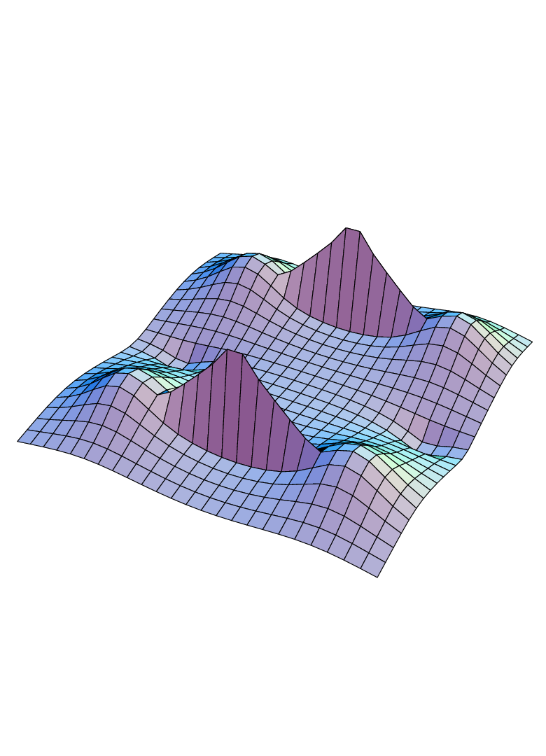
Calorons, however, have an additional feature. When squeezed in the imaginary time direction (the size $\rho$ becoming bigger than the period $\beta$), they split in constituent monopoles with masses $8\pi^{2}\nu_{j}/\beta$ ($\nu_{j}\equiv\mu_{j+1}-\mu_{j}$). Outside the cores of these monopoles the gauge field becomes abelian. Ignoring the charged components, which decay exponentially outside the cores of the constituent monopoles, the field is described in terms of self-dual Dirac monopoles. The singularity of a Dirac string can only be avoided by not neglecting the contributions coming from the charged components, even when far away from the constituents. For a single caloron we would not care, since the Dirac string is not seen in gauge invariant quantities. It does, however, involve a rather subtle interplay between the charged and neutral components of the gauge field in the vicinity of the would-be Dirac string [1]. It is this subtle interplay that is disturbed when we add gauge fields of various calorons together. Unlike for the gauge singularity, the combined field will not diverge, but it shows a narrow and steep enhancement at the location of the would-be Dirac string as illustrated in Fig. 1, where we added two $SU(2)$ calorons. Also here one may shield the Dirac strings from these tails. But one always pays the price that the Dirac string no longer can be hidden, and carries energy. Let us stress again that these are genuine gauge invariant non-singular features in the configuration, even though they are of course a consequence of our particular way of constructing a superposition.

A visible would-be Dirac string presents a formidable obstacle to considering the constituents as independent objects; they remember to which caloron they belong. Insisting the abelian field far from the constituents to be exactly additive under the approximate superposition leaves us little room for considering other possible superpositions, apart from carefully fine-tuning the charged components of the configuration. Solving for the exact self-dual caloron solutions of higher charge we wish to show that a visible Dirac string is an artifact of the particular procedure to construct approximate caloron solutions. For the exact charge $k$ caloron solutions we expect $kn$ constituents and from the point of view of the parameter space these can be expected to be independent (as long the constituents do not get too close together).

In this paper we develop the formalism and give exact solutions for a class of axially symmetric solutions. For $SU(2)$ an example of such an exact solution with charge 2 is presented in Fig. 2. We compare the exact solution (left), with the one obtained by adding two charge 1 calorons, showing the would-be Dirac strings (middle) and with the exact abelian solution determined from (self-dual) Dirac monopoles placed at the location of the constituents (right). Indeed, the would-be Dirac strings are no longer visible for the exact non-abelian solution. This gives us good reasons to expect that moving away from the requirement of axial symmetry, the exact solutions will exhibit the constituent monopoles as independent objects. This is an important prerequisite for attempting to formulate the long distance features of QCD in terms of these monopoles. Non-linearities will remain important when constituents overlap, like for instantons at zero-temperature, as will be illustrated through suitable examples.

Our results can also be used to extract information on multi-monopole solutions. In the charge 1 case it has been shown [1] that sending one of the constituents to infinity one is left with exact monopole solutions. Perhaps somewhat surprisingly, it has been notoriously difficult to construct approximate superpositions of magnetic monopoles in such a way the interaction energy decreases with their separation. Within our approach this is due to the difficulty (particularly when sending some constituents to infinity) in keeping Dirac strings hidden. It would therefore still be important to find approximate superpositions that achieve this. Nevertheless, it shows how subtle it is to consider abelian fields as embedded in non-abelian ones. There is much more to ’t Hooft’s abelian projection [7] than meets the eye at first glance.

The rest of the paper will be organized as follows. In Sect. 2 we formulate the Fourier analysis of the ADHM data for calorons of higher charge. This allows us in Sect. 2.1 to relate to the Nahm equations, providing the connection between the ADHM and Nahm data. The Nahm equation for charge $k$ calorons [4] expresses self-duality of dual $SU(k)$ gauge fields on a circle, but with singularities. In Sect. 2.2 we introduce the “master” Green’s function in terms of which the gauge field (Sect. 2.3) and the action density (Sect. 2.4) can be explicitly computed, relying heavily on some beautiful results [8, 9] derived in the context of the ADHM construction.

This can all be achieved without explicitly solving the Nahm equation. In Sect. 3 we will, however, solve it for some special cases with axial symmetry. There we also illustrate some interesting features that appear when constituents overlap, similar to what was observed at zero temperature [10].

Sect. 4 is devoted to the far-field limit (related to the high-temperature limit), where up to exponential corrections only the abelian component of the field survives. Again, expressions can be derived without explicitly solving the Nahm equation. We apply the formalism to the exact axially symmetric solutions in Sect. 4.3.1, where we prove that in the far-field region they are in a precise sense described by (self-dual) Dirac monopoles, which is conjectured to be the case for any exact solution.

We end in Sect. 5 with a discussion of lattice results that have been obtained by various groups, some open questions and suggestions for future studies.

In constructing the higher charge caloron solutions similar steps are followed as for charge 1. We distinguish two constructions, $Sp(n)$ based on quaternions, and $SU(n)$ based on complex spinors. With $SU(2)=Sp(1)$, this implies that for $SU(2)$ two constructions are possible. For $k=1$ it was easily shown these are identical, but for $k>1$ this is more complicated due to the quadratic ADHM constraint [3] which can not be solved in all generality. Since the essential part of the construction that employs the impurity scattering technique is identical in both approaches, we will give a unified presentation.

The $SU(n)$ ADHM formalism for charge $k$ instantons [3] employs a $k$ dimensional vector $\lambda=(\lambda_{1},\ldots,\lambda_{k})$, where $\lambda_{i}^{\dagger}$ is a two-component spinor in the $\bar{n}$ representation of $SU(n)$. Alternatively, $\lambda$ can be seen as a $n\times 2k$ complex matrix. In addition one has four complex hermitian $k\times k$ matrices $B_{\mu}$, combined into a $2k\times 2k$ complex matrix $B=\sigma_{\mu}\otimes B_{\mu}$, using the unit quaternions $\sigma_{\mu}=({\Eins}_{2},i\vec{\tau})$ and $\bar{\sigma}_{\mu}=({\Eins}_{2},-i\vec{\tau})$, where $\tau_{i}$ are the Pauli matrices. With some abuse of notation, we often write $B=\sigma_{\mu}B_{\mu}$. Together $\lambda$ and $B$ constitute the $(n+2k)\times 2k$ dimensional matrix $\Delta(x)$, to which is associated a complex $(n+2k)\times n$ dimensional normalized zero mode vector $v(x)$,

Here the quaternion $x=x_{\mu}\sigma_{\mu}$ denotes the position (a $k\times k$ unit matrix is implicit) and $v(x)$ can be solved explicitly in terms of the ADHM data by

As $\phi(x)$ is an $n\times n$ positive hermitian matrix, its square root $\phi^{{\scriptstyle{{1\over 2}}}}(x)$ is well-defined. The gauge field is given by

The $Sp(1)$ ADHM formalism for charge $k$ instantons [3] employs also a $k$ dimensional vector $\lambda=(\lambda_{1},\ldots,\lambda_{k})$, where now $\lambda_{i}$ is a quaternion (4 real parameters). Again, $\lambda$ can be seen as an $2\times 2k$ complex matrix (but with $4k$ real, as opposed to complex, parameters). Now the four $k\times k$ matrices $B_{\mu}$ are required to be real and symmetric, still to be combined into a $2k\times 2k$ complex matrix $B=\sigma_{\mu}B_{\mu}$. The $(2+2k)\times 2k$ dimensional matrix $\Delta(x)$ is constructed as before. It is immediately obvious that now $\phi(x)$ is proportional to $\sigma_{0}$, simplifying the expression for the gauge field to

For $A_{\mu}(x)$ to be a self-dual connection, $\Delta(x)$ has to satisfy the quadratic ADHM constraint, which states that $\Delta^{\dagger}(x)\Delta(x)=B^{\dagger}(x)B(x)+\lambda^{\dagger}\lambda$ (considered as a $k\times k$ complex quaternionic matrix) has to commute with the quaternions, or equivalently

defining $f_{x}$ as a hermitian (resp. symmetric) $k\times k$ Green’s function. The self-duality follows by computing the curvature

making essential use of the fact that $f_{x}$ commutes with the quaternions, and $\eta_{\mu\nu}\equiv\sigma_{[\mu}\bar{\sigma}_{\nu]}$ being self-dual ($\bar{\eta}_{\mu\nu}\equiv\bar{\sigma}_{[\mu}\sigma_{\nu]}$ is anti-selfdual). The quadratic constraint can be formulated as ${\Im m}(\Delta^{\dagger}(x)\Delta(x))=0$, where ${\Im m}W\equiv W-{\scriptstyle{{1\over 2}}}\sigma_{0}{\rm tr}_{2}W$, and one obtains

where ${\rm tr}_{2}$ is the spinorial trace. Note that this implies that ${\rm tr}_{2}(\tau_{a}\lambda^{\dagger}\lambda)$ is traceless for $a=1,2,3$.

To count the number of instanton parameters we observe that the transformation $\lambda\rightarrow\lambda T^{\dagger}$, $B_{\mu}\rightarrow TB_{\mu}T^{\dagger}$, with $T\in U(k)$ (resp. $T\in O(k)$) leaves the gauge field and the ADHM constraint untouched. Taking this symmetry into account, one checks the dimension of the instanton moduli space to be $4kn$ dimensional. We have $4kn$ and $4k^{2}$ real parameters from $\lambda$ and $B_{\mu}$. The $U(k)$ symmetry removes $k^{2}$ real parameters and finally the quadratic ADHM constraint gives $3k^{2}$ real equations. On the other hand, for the quaternionic construction there are $4k$ and $4\cdot{\scriptstyle{{1\over 2}}}k(k+1)$ parameters from $\lambda$ and $B_{\mu}$, of which ${\scriptstyle{{1\over 2}}}k(k-1)$ are removed by the $O(k)$ symmetry, and the quadratic ADHM constraint gives $3\cdot{\scriptstyle{{1\over 2}}}k(k-1)$ equations. Global gauge transformations are realized by $\lambda\rightarrow g\lambda$, with $g\in SU(n)$ and are here included in the parameter count. For calorons with non-trivial holonomy the dimension of the gauge invariant parameter space is minimally reduced by $n-1$ (maximal symmetry breaking) and maximally by $n^{2}-1$ (trivial holonomy).

We note that for $SU(2)$ the quadratic ADHM constraint and symmetry of the ADHM data for high charge differ considerably. For the caloron we have to deal in a sense with infinite topological charge, but finite within each (imaginary) time interval of length $\beta$. This infinity is resolved by Fourier transformation, relating it to the Nahm formalism [4], but the difference between the $U(k)$ and $O(k)$ symmetries (the infinity is moved to making these gauge symmetries local) remains, as well as of course the nature of the Nahm data (the Fourier transformation of the ADHM data). Henceforth we put $\beta=1$, which can always be achieved by a rescaling.

Like for charge one [1, 2] the caloron with Polyakov loop ${{\cal P}_{\infty}}$ at infinity is built out of a periodic array of instantons, twisted by ${{\cal P}_{\infty}}$. This is implemented in the ADHM formalism by requiring (suppressing color and spinor indices, respectively quaternion indices)

with $p\in{\mathbb{Z}}$ (the Fourier index), and $a=1,\ldots,k$ (associated to the non-Abelian nature of the Nahm data). Using that $\phi^{\pm{\scriptstyle{{1\over 2}}}}(x+1)={{\cal P}_{\infty}}\phi^{\pm{\scriptstyle{{1\over 2}}}}(x){\cal{P}}_{\infty}^{-1}$, Eq. (4) leads to the required periodicity. Demanding

suitably implements Eq. (9) and is partially solved by imposing

with $\hat{A}$ still to be determined to account for Eq. (8). It is useful to introduce the $n$ projectors $P_{m}$ on the $m$th eigenvalue of ${{\cal P}_{\infty}}$, such that ${{\cal P}_{\infty}}=\sum_{m}e^{2\pi i\mu_{m}}P_{m}$ and $\lambda_{pk+a}=\sum_{m}e^{2\pi ip\mu_{m}}P_{m}\zeta_{a}$.

References

- [1] T.C. Kraan and P. van Baal, Phys. Lett. B428 (1998) 268 [hep-th/9802049]; Nucl. Phys. B533 (1998) 627 [hep-th/9805168].
- [2] T.C. Kraan and P. van Baal, Phys. Lett. B435 (1998) 389 [hep-th/9806034].
- [3] M.F. Atiyah, N.J. Hitchin, V.G. Drinfeld, Yu. I. Manin, Phys. Lett. 65 A (1978) 185; M.F. Atiyah, Geometry of Yang-Mills fields, Fermi lectures, (Scuola Normale Superiore, Pisa, 1979).
- [4] W. Nahm, Self-dual monopoles and calorons, in: Lect. Notes in Physics. 201, eds. G. Denardo, e.a. (1984) p. 189.
- [5] K. Lee and P. Yi, Phys. Rev. D56 (1997) 3711 (hep-th/9702107); K. Lee, Phys. Lett. B426 (1998) 323 [hep-th/9802012]; K. Lee and C. Lu, Phys. Rev. D58 (1998) 025011 (hep-th/9802108).
- [6] W. Nahm, Phys. Lett. 90B (1980) 413.
- [7] G. ’t Hooft, Nucl. Phys. B190 [FS3] (1981) 455; Physica Scripta 25 (1982) 133.
- [8] E.F. Corrigan, D.B. Fairlie, S. Templeton and P. Goddard, Nucl. Phys. B140 (1978) 31.
- [9] H. Osborn, Nucl. Phys. B159 (1979) 497.
- [10] M. García Pérez, T.G. Kovács and P. van Baal, Phys. Lett. B472 (2000) 295 [hep-ph/9911485].
- [11] P. van Baal, in: Lattice fermions and structure of the vacuum, eds. V. Mitrjushkin and G. Schierholz (Kluwer, Dordrecht, 2000), p. 269 [hep-th/9912035].
- [12] K. Lee, E.J. Weinberg and P. Yi, Phys. Lett. B376 (1996) 97 (hep-th/9601097); Phys. Rev. D54 (1996) 6351 (hep-th/9605229); E.J. Weinberg, Massive and Massless Monopoles and Duality, hep-th/9908095.
- [13] T.C. Kraan, Comm. Math. Phys. 212 (2000) 503 [hep-th/9811179].
- [14] B.J. Harrington and H.K. Shepard, Phys. Rev. D17 (1978) 2122; ibid. D18 (1978) 2990.
- [15] P. Rossi, Nucl. Phys. B149 (1979) 170.
- [16] M. García Pérez, A. González-Arroyo, A. Montero and P. van Baal, Jour. of High Energy Phys. 06 (1999) 001 [hep-lat/9903022)].
- [17] M. García Pérez, A. González-Arroyo, C. Pena and P. van Baal, Phys. Rev. D60 (1999) 031901 [hep-th/9905016].
- [18] M.N. Chernodub, T.C. Kraan and P. van Baal, Nucl. Phys. B(Proc.Suppl.) 83-84 (2000) 556 [hep-lat/9907001].
- [19] M. García Pérez, A. González-Arroyo, C. Pena and P. van Baal, Nucl. Phys. B564 (1999) 159 [hep-th/9905138].
- [20] E.-M. Ilgenfritz, M. Müller-Preussker, and A.I. Veselov, in: Lattice fermions and structure of the vacuum, eds. V. Mitrjushkin and G. Schierholz (Kluwer, Dordrecht, 2000), 345 [hep-lat/0003025].
- [21] E.-M. Ilgenfritz, B.V. Martemyanov, M. Müller-Preussker and A.I. Veselov, Nucl. Phys. B(Proc.Suppl.)94 (2001) 407 [hep-lat/0011051]; Nucl. Phys. B(Proc. Suppl.)106 (2002) 589 [hep-lat/0110212].
- [22] M.L. Laursen and G. Schierholz, Z. Phys. C38 (1988) 501.
- [23] E.-M. Ilgenfritz, B.V. Martemyanov, M. Müller-Preussker, S. Shcherendin and A.I. Veselov, hep-lat/0206004.
- [24] P. van Baal, Nucl. Phys. B(Proc.Suppl.)106 (2002) 586 [hep-lat/0108027].
- [25] C. Gattringer, M. Göckeler, P.E.L. Rakow, S. Schaefer, A. Schäfer, Nucl. Phys. B618 (2001) 205 [hep-lat/0105023].
- [26] Christof Gattringer, private communications. The zero-mode densities for the case of Fig. 7 were produced for the purpose of illustrating the behavior observed by C. Gattringer and co-workers in lattice gauge theory.
- [27] T.C. Kraan and P. van Baal, Nucl. Phys. B(Proc. Suppl.)73 (1999) 554 [hep-lat/9808015].
- [28] www.lorentz.leidenuniv.nl/vanbaal/Caloron.html
- [29] P. van Baal, Chiral zero-modes for abelian BPS dipoles, to appear in “Confinement, Topology, and other Non-Perturbative Aspects of QCD”, eds. J. Greensite and S. Olejnik (Kluwer), hep-th/0202182.