Testing quantum chromodynamics to high precision is not easy. Even in processes involving high momentum transfer, perturbative QCD predictions are complicated by questions of the convergence of the series, particularly by the presence of “renormalon” terms which grow as $n!$, reflecting the uncertainty in the analytic form of the QCD coupling at low scales. Virtually all QCD processes are complicated by the presence of dynamical higher twist effects, including power-law suppressed contributions due to multi-parton correlations, intrinsic transverse momentum, and finite quark masses. Many of these effects are inherently nonperturbative in nature and require knowledge of hadron wavefunction themselves. The problem of interpreting perturbative QCD predictions is further compounded by theoretical ambiguities due to the apparent freedom in the choice of renormalization schemes, renormalization scales, and factorization procedures.

A central principle of renormalization theory is that predictions which relate physical observables to each other cannot depend on theoretical conventions. For example, one can use any renormalization scheme, such as the modified minimal subtraction scheme, and any choice of renormalization scale $\mu$ to compute perturbative series relating observables $A$ and $B$. However, all traces of the choices of the renormalization scheme and scale must disappear when one algebraically eliminates the $\alpha_{\overline{\mbox{MS}}}(\mu)$ and directly relate $A$ to $B$. This is the principle underlying “commensurate scale relations” (CSR),[1] which are general leading-twist QCD predictions relating physical observables to each other. For example, the “generalized Crewther relation”, which is discussed in more detail below, provides a scheme-independent relation between the QCD corrections to the Bjorken (or Gross Llewellyn-Smith) sum rule for deep inelastic lepton-nucleon scattering, at a given momentum transfer $Q$, to the radiative corrections to the annihilation cross section $\sigma_{e^{+}e^{-}\to\rm hadrons}(s)$, at a corresponding “commensurate” energy scale $\sqrt{s}$. [1, 2] The specific relation between the physical scales $Q$ and $\sqrt{s}$ reflects the fact that the radiative corrections to each process have distinct quark mass thresholds.

Any perturbatively calculable physical quantity can be used to define an effective charge[3, 4, 5] by incorporating the entire radiative correction into its definition. For example, the $e^{+}e^{-}\to\gamma^{*}\to{\rm hadrons}$ to muon pair cross section ratio can be written $(C_{F}=(N^{2}_{C}-1)/2N_{C})$

where $R^{0}_{e^{+}e^{-}}$ is the prediction at Born level. Similarly, one can define the entire radiative correction to the Bjorken sum rule as the effective charge $\alpha_{g_{1}}(Q^{2})$ where $Q$ is the corresponding momentum transfer:

By convention, each effective charge is normalized to $\alpha_{s}$ in the weak coupling limit. One can define effective charges for virtually any quantity calculable in perturbative QCD; e.g. moments of structure functions, ratios of form factors, jet observables, and the effective potential between massive quarks. In the case of decay constants of the $Z$ or the $\tau$, the mass of the decaying system serves as the physical scale in the effective charge. In the case of multi-scale observables, such as the two-jet fraction in $e^{+}e^{-}$ annihilation, the multiple arguments of the effective coupling $\alpha_{2jet}(s,y)$ correspond to the overall available energy $s$ and variables such as $y=\rm{max}_{ij}(p_{i}+p_{j})^{2}/s$ representing the maximum jet mass fraction.

Commensurate scale relations take the general form

The function $C_{AB}(\alpha_{B})$ relates the observables $A$ and $B$ in the conformal limit; i.e., $C_{AB}$ gives the functional dependence between the effective charges which would be obtained if the theory had zero $\beta$ function. The conformal coefficients $c_{n}^{AB}$ can be distinguished from the terms associated with the $\beta$ function at each order in perturbation theory from their color and flavor dependence, or by an expansion about a fixed point.

The ratio of commensurate scales $\Lambda_{BA}$ is determined by the requirement that all terms involving the $\beta$ function are incorporated into the arguments of the running couplings, as in the original BLM procedure.[6] Physically, the ratio of scales corresponds to the fact that the physical observables have different quark threshold and distinct sensitivities to fermion loops. More generally, the differing scales are in effect relations between mean values of the physical scales which appear in loop integrations. Commensurate scale relations are transitive; i.e., given the relation between effective charges for observables $A$ and $C$ and $C$ and $B$, the resulting between $A$ and $B$ is independent of $C$. In particular, transitivity implies $\Lambda_{AB}=\Lambda_{AC}\times\Lambda_{CB}$. The shift in scales which gives conformal coefficients in effect pre-sums the large and strongly divergent terms in the PQCD series which grow as $n!(\beta_{0}\alpha_{s})^{n}$, i.e., the infrared renormalons associated with coupling-constant renormalization.[7, 8, 9, 10]

One can consider QCD predictions as functions of analytic variables of the number of colors $N_{C}$ and flavors $N_{F}$. For example, one can show at all orders of perturbation theory that PQCD predictions reduce to those of an Abelian theory at $N_{C}\to 0$ with $C_{F}\alpha_{s}$ and $N_{F}/T_{F}C_{F}$ held fixed, where $C_{F}=4/3$ and $T_{F}=1/2$ for QCD. In particular, CSRs obey the “Abelian correspondence principle” in that they give the correct Abelian relations at $N_{C}\to 0.$ [6, 11, 12, 13, 14]

Similarly, commensurate scale relations obey the “conformal correspondence principle”: the CSRs reduce to correct conformal relations when $N_{C}$ and $N_{F}$ are tuned to produce zero $\beta$ function. Thus conformal symmetry provides a template for QCD predictions, providing relations between observables which are present even in theories which are not scale invariant. All effects of the nonzero beta function are encoded in the appropriate choice of relative scales $\Lambda_{AB}=Q_{A}/Q_{B}$.

The scale $Q$ which enters a given effective charge corresponds to a physical momentum scale. The total logarithmic derivative of each effective charge $\alpha_{A}(Q)$ with respect to its physical scale is given by the Gell Mann-Low equation:

where the functional dependence of $\Psi_{A}$ is specific to its own effective charge. Here $m$ refers to the quark’s pole mass. The pole mass is universal in that it does not depend on the choice of effective charge. The Gell Mann-Low relation is reflexive in that $\Psi_{A}$ depends on only on the coupling $\alpha_{A}$ at the same scale. It should be emphasized that the Gell Mann-Low equation deals with physical quantities and is independent of the renormalization procedure and choice of renormalization scale. A central feature of quantum chromodynamics is asymptotic freedom; i.e., the monotonic decrease of the QCD coupling $\alpha_{A}(Q)$ at large spacelike scales. The empirical test of asymptotic freedom is the verification of the negative sign of the Gell Mann-Low function at large momentum transfer, which must be true for any effective charge.

In perturbation theory,

At large scales $Q^{2}\gg m^{2}$, the first two terms are universal and identical to the first two terms of the $\beta$ function $\psi_{A}^{\{0\}}=\beta_{0}={11N_{C}\over 6}-{2\over 3}T_{F}N_{F},\psi_{A}^{\{1\}}=\beta_{1}={17\over 12}C_{A}^{2}-{5\over 6}C_{A}T_{F}N_{F}-{1\over 2}C_{F}T_{F}N_{F},$ whereas $\psi_{A}^{\{n\}}$ for $n\geq 2$ are process dependent. The quark mass dependence of the $\Psi$ function is analytic, and in the case of the $\alpha_{V}$ scheme is known to two loops.[15] Collecting all the mass effects into a mass dependent function $N_{F}$ gives the effective number of flavors in the V-scheme; $\psi_{V}^{\{0\}}\left(Q/m\right)=\frac{11}{2}-\frac{1}{3}N_{F,V}^{\{0\}}\left(Q/m\right)$ and $\psi_{V}^{\{1\}}\left(Q/m\right)=\frac{51}{4}-\frac{19}{12}N_{F,V}^{\{1\}}\left(Q/m\right)$, with the subscript $V$ indicating the scheme dependence.

The commensurate scale relation between $\alpha_{A}$ and $\alpha_{B}$ implies an elegant relation between their conformal dependence $C_{AB}$ and their respective Gell Mann Low functions:

Thus given the result for $N_{F,V}(m/Q)$ in the $\alpha_{V}$ scheme one can use the CSR to derive $N_{F,A}(m/Q)$ for any other effective charge, at least to two loops. The above relation also shows that if one effective charge has a fixed point $\Psi_{A}[\alpha_{A}(Q^{FP}_{A})]=0$, then all effective charges $B$ have a corresponding fixed point $\Psi_{B}[\alpha_{B}(Q^{FP}_{B})]=0$ at the corresponding commensurate scale and value of effective charge.

In quantum electrodynamics, the running coupling $\alpha_{QED}(Q^{2})$, defined from the Coulomb scattering of two infinitely heavy test charges at the momentum transfer $t=-Q^{2}$, is taken as the standard observable. Is there a preferred effective charge which one should use to characterize the coupling strength in QCD? In the case of QCD, the heavy-quark potential $V(Q^{2})$ is customarily defined via a Wilson loop from the interaction energy of infinitely heavy quark and antiquark at momentum transfer $t=-Q^{2}.$ The relation $V(Q^{2})=-4\pi C_{F}\alpha_{V}(Q^{2})/Q^{2}$ then defines the effective charge $\alpha_{V}(Q).$ As in the corresponding case of Abelian QED, the scale $Q$ of the coupling $\alpha_{V}(Q)$ is identified with the exchanged momentum. Thus there is never any ambiguity in the interpretation of the scale. All virtual corrections due to fermion pairs are incorporated in $\alpha_{V}$ through loop diagrams which depend on the physical mass thresholds. Other observables could be used to define the standard QCD coupling, such as the effective charge defined from heavy quark radiation.[16]

Commensurate scale relations between $\alpha_{V}$ and the QCD radiative corrections to other observables have no scale or scheme ambiguity, even in multiple-scale problems such as multi-jet production. As is the case in QED, the momentum scale which appears as the argument of $\alpha_{V}$ reflect the mean virtuality of the exchanged gluons. Furthermore, one can write a commensurate scale relation between $\alpha_{V}$ and an analytic extension of the $\alpha_{\overline{\mbox{MS}}}$ coupling, thus transferring most of the unambiguous scale-fixing and analytic properties of the physical $\alpha_{V}$ scheme to the $\overline{\mbox{MS}}$ coupling.

Some examples of CSR’s at NNLO are given by:

For numerical purposes in each case $N_{F}=5$ and $\alpha_{V}=0.1$ have been used to compute the NLO correction to the CSR scale.

Commensurate scale relations thus provide fundamental and precise scheme-independent tests of QCD, predicting how observables track not only in relative normalization, but also in their commensurate scale dependence.

The generalized Crewther relation[2] can be derived by calculating the QCD radiative corrections to the deep inelastic sum rules and $R_{e^{+}e^{-}}$ in a convenient renormalization scheme such as the modified minimal subtraction scheme $\overline{\rm MS}$. One then algebraically eliminates $\alpha_{\overline{\mbox{MS}}}(\mu)$. Finally, BLM scale-setting[6] is used to eliminate the $\beta$-function dependence of the coefficients. The form of the resulting relation between the observables thus matches the result which would have been obtained had QCD been a conformal theory with zero $\beta$ function. The final result relating the observables is independent of the choice of intermediate $\overline{\rm MS}$ renormalization scheme.

More specifically, consider the Adler function[17] for the $e^{+}e^{-}$ annihilation cross section

The entire radiative correction to this function is defined as the effective charge $\alpha_{D}(Q^{2})$:

The coefficient $C_{\rm L}(Q^{2})$ appears at the third order in perturbation theory and is related to the “light-by-light scattering type” diagrams.

It is straightforward to algebraically relate $\alpha_{g_{1}}(Q^{2})$ to $\alpha_{D}(Q^{2})$ using the known expressions to three loops in the $\overline{\rm MS}$ scheme. If one chooses the renormalization scale to resum all the corrections due to the running of the coupling into $\alpha_{D}(Q^{2})$, then the final result turns out to be remarkably simple[2] $(\widehat{\alpha}=3/4\,C_{F}\ \alpha/\pi):$

where

This relation shows how the coefficient functions for these two different processes are related to each other at their respective commensurate scales. We emphasize that the $\overline{\mbox{MS}}$ renormalization scheme is used only for calculational convenience; it serves simply as an intermediary between observables. The renormalization group ensures that the forms of the CSR relations in perturbative QCD are independent of the choice of an intermediate renormalization scheme.

The Crewther relation was originally derived assuming that the theory is conformally invariant; i.e., for zero $\beta$ function. In the physical case, where the QCD coupling runs, all non-conformal effects are resummed into the energy and momentum transfer scales of the effective couplings $\alpha_{R}$ and $\alpha_{g1}$. The general relation between these two effective charges for non-conformal theory thus takes the form of a geometric series

We have dropped the small light-by-light scattering contributions. This is again a special advantage of relating observable to observable. The coefficients are independent of color and are the same in Abelian, non-Abelian, and conformal gauge theory. The non-Abelian structure of the theory is reflected in the expression for the scale ${Q}^{*}$.

Is experiment consistent with the generalized Crewther relation? Fits [18] to the experimental measurements of the $R$-ratio above the thresholds for the production of $c\overline{c}$ bound states provide the empirical constraint: $\alpha_{R}({\sqrt{s}}=5.0~{\rm GeV})/\pi\simeq 0.08\pm 0.03.$ The prediction for the effective coupling for the deep inelastic sum rules at the commensurate momentum transfer $Q$ is then $\alpha_{g_{1}}(Q=12.33\pm 1.20~{\rm GeV})/\pi\simeq\alpha_{\rm GLS}(Q=12.33\pm 1.20~{\rm GeV})/\pi\simeq 0.074\pm 0.026.$ Measurements of the Gross-Llewellyn Smith sum rule have so far only been carried out at relatively small values of $Q^{2}$;[19, 20] however, one can use the results of the theoretical extrapolation[21] of the experimental data presented in:[22] $\alpha_{\rm GLS}^{\rm extrapol}(Q=12.25~{\rm GeV})/\pi\simeq 0.093\pm 0.042.$ This range overlaps with the prediction from the generalized Crewther relation. It is clearly important to have higher precision measurements to fully test this fundamental QCD prediction.

In general, one can write the relation between any two effective charges at arbitrary scales $Q_{A}$ and $Q_{B}$ as a correction to the corresponding relation obtained in a conformally invariant theory:

where

is the functional relation when $\Psi_{B}[\alpha_{B}]=0$. In fact, if $\alpha_{B}$ approaches a fixed point $\bar{\alpha}_{B}$ where $\Psi_{B}[\bar{\alpha}_{B}]=0$, then $\alpha_{A}$ tends to a fixed point given by

The commensurate scale relation for observables $A$ and $B$ has a similar form, but in this case the relative scales $\Lambda_{BA}=Q_{B}/Q_{A}$ are fixed such that the non-conformal term $D^{AB}$ is zero. Thus the commensurate scale relation $\alpha_{A}(Q_{A})=C^{AB}[\alpha_{B}(\Lambda_{BA}Q_{A})]$ at general commensurate scales is also the relation connecting the values of the fixed points for any two effective charges or schemes. Furthermore, as $\Psi\rightarrow 0$, the ratio of commensurate scales $Q^{2}_{A}/Q^{2}_{B}$ becomes the ratio of fixed point scales $\bar{Q}^{2}_{A}/\bar{Q}^{2}_{B}$ as one approaches the fixed point regime.

The effective charge $\alpha_{V}(Q)$ provides a physically-based alternative to the usual modified minimal subtraction ($\overline{\mbox{MS}}$) scheme. All virtual corrections due to fermion pairs are incorporated in $\alpha_{V}$ through loop diagrams which depend on the physical mass thresholds. When continued to time-like momenta, the coupling has the correct analytic dependence dictated by the production thresholds in the crossed channel. Since $\alpha_{V}$ incorporates quark mass effects exactly, it avoids the problem of explicitly computing and resumming quark mass corrections which are related to the running of the coupling. Thus the effective number of flavors $N_{F}(Q/m)$ is an analytic function of the scale $Q$ and the quark masses $m$. The effects of finite quark mass corrections on the running of the strong coupling were first considered by De Rújula and Georgi[23] within the momentum subtraction schemes (MOM) (see also references[24, 25, 26, 27]). The two-loop calculation was first done by Yoshino and Hagiwara[28] in the MOM-scheme using Landau gauge and was also recently calculated by Jegerlehner and Tarasov[29] using background field gauge.

One important advantage of the physical charge approach is its inherent gauge invariance to all orders in perturbation theory. This feature is not manifest in massive $\beta$-functions defined in non-physical schemes such as the MOM schemes. A second, more practical, advantage is the automatic decoupling of heavy quarks according to the Appelquist-Carazzone theorem.[30]

The specification of the coupling and renormalization scheme also depends on the definition of the quark mass. In contrast to QED where the on-shell mass provides a natural definition of lepton masses, an on-shell definition for quark masses is complicated by the confinement property of QCD. For a physical charge it is natural to use the pole mass $m$ which has the advantage of being scheme and renormalization-scale invariant as well as giving explicit decoupling.

In a recent paper[15] with M. Melles we have presented a two-loop analytic extension of the $\alpha_{V}$-scheme based on previous results.[31] The mass effects are in principle treated exactly to two-loop order and are only limited in practice by the uncertainties from numerical integration. The desired features of gauge invariance and decoupling are manifest in the form of the two-loop Gell-Mann Low function. Strong consistency checks of the results are performed by comparing the Abelian limit to the well known QED results in the on-shell scheme. In addition, the massless as well as the decoupling limit are reproduced exactly, and the two-loop Gell-Mann Low function is shown to be renormalization scale ($\mu$) independent.

The results of the numerical calculation of $N_{F,V}^{(1)}$ in the $V$-scheme for QCD and QED are shown in Fig. 1. The decoupling of heavy quarks becomes manifest at small $Q/m$, and the massless limit is attained for large $Q/m$. The QCD form actually becomes negative at moderate values of $Q/m$, a novel feature of the anti-screening non-Abelian contributions. This property is also present in the (gauge dependent) MOM results. In contrast, in Abelian QED the two-loop contribution to the effective number of flavors becomes larger than one at intermediate values of $Q/m$. The figure also displays the one-loop contribution $N^{(0)}_{F,V}\left(Q/m\right)$ which monotonically interpolates between the decoupling and massless limits. The solid curves displayed in Fig. 1 shows simple parameterizations of $N_{F,V}^{(1)}$ which can be used to get a simple representation of the numerical results.

By employing the commensurate scale relations, other physical observables can be expressed in terms of the analytic coupling $\alpha_{V}$ without scale or scheme ambiguity. This way the quark mass threshold effects in the running of the coupling are taken into account by utilizing the mass dependence of the physical $\alpha_{V}$ scheme. In effect, quark thresholds are treated analytically to all orders in $m^{2}/Q^{2}$; i.e., the evolution of the physical $\alpha_{V}$ coupling in the intermediate regions reflects the actual mass dependence of a physical effective charge and the analytic properties of particle production. Furthermore, the definiteness of the dependence in the quark masses automatically constrains the scale $Q$ in the argument of the coupling. There is thus no scale ambiguity in perturbative expansions in $\alpha_{V}$.

The use of $\alpha_{V}$ and related physically defined effective charges such as the plaquette charge $\alpha_{P}$ (to NLO the effective charge defined from the (1,1) plaquette, $\alpha_{P}$ is the same as $\alpha_{V}$) as expansion parameters has been found to be valuable in lattice gauge theory, greatly increasing the convergence of perturbative expansions relative to those using the bare lattice coupling.[12] Recent lattice calculations of the $\Upsilon$- spectrum[32] have been used with BLM scale-fixing to determine a NLO normalization of the static heavy quark potential: $\alpha_{V}^{(3)}(8.2{\rm GeV})=0.196(3)$ where the effective number of light flavors is $N_{F}=3$. The corresponding modified minimal subtraction coupling evolved to the $Z$ mass and five flavors is $\alpha_{\overline{MS}}^{(5)}(M_{Z})=0.1174(24)$. Thus a high precision value for $\alpha_{V}(Q^{2})$ at a specific scale is available from lattice gauge theory. Predictions for other QCD observables can be directly referenced to this value without the scale or scheme ambiguities, thus greatly increasing the precision of QCD tests.

One can also use $\alpha_{V}$ to characterize the coupling which appears in the hard scattering contributions of exclusive process amplitudes at large momentum transfer, such as elastic hadronic form factors, the photon-to-pion transition form factor at large momentum transfer[6, 33] and exclusive weak decays of heavy hadrons.[34] Each gluon propagator with four-momentum $k^{\mu}$ in the hard-scattering quark-gluon scattering amplitude $T_{H}$ can be associated with the coupling $\alpha_{V}(k^{2})$ since the gluon exchange propagators closely resembles the interactions encoded in the effective potential $V(Q^{2})$. [In Abelian theory this is exact.] Commensurate scale relations can then be established which connect the hard-scattering subprocess amplitudes which control exclusive processes to other QCD observables.

We can anticipate that eventually nonperturbative methods such as lattice gauge theory or discretized light-cone quantization will provide a complete form for the heavy quark potential in QCD. It is reasonable to assume that $\alpha_{V}(Q)$ will not diverge at small space-like momenta. One possibility is that $\alpha_{V}$ stays relatively constant $\alpha_{V}(Q)\simeq 0.4$ at low momenta, consistent with fixed-point behavior. There is, in fact, empirical evidence for freezing of the $\alpha_{V}$ coupling from the observed systematic dimensional scaling behavior of exclusive reactions.[33] If this is in fact the case, then the range of QCD predictions can be extended to quite low momentum scales, a regime normally avoided because of the apparent singular structure of perturbative extrapolations.

There are a number of other advantages of the $V$-scheme:

1. 1.

   Perturbative expansions in $\alpha_{V}$ with the scale set by the momentum transfer cannot have any $\beta$-function dependence in their coefficients since all running coupling effects are already summed into the definition of the potential. Since coefficients involving $\beta_{0}$ cannot occur in an expansions in $\alpha_{V}$, the divergent infrared renormalon series of the form $\alpha^{n}_{V}\beta_{0}^{n}n!$ cannot occur. The general convergence properties of the scale $Q^{*}$ as an expansion in $\alpha_{V}$ is not known.[8]

2. 2.

   The effective coupling $\alpha_{V}(Q^{2})$ incorporates virtual contributions with finite fermion masses. When continued to time-like momenta, the coupling has the correct analytic dependence dictated by the production thresholds in the $t$ channel. Since $\alpha_{V}$ incorporates quark mass effects exactly, it avoids the problem of explicitly computing and resumming quark mass corrections.

3. 3.

   The $\alpha_{V}$ coupling is the natural expansion parameter for processes involving non-relativistic momenta, such as heavy quark production at threshold where the Coulomb interactions, which are enhanced at low relative velocity $v$ as $\pi\alpha_{V}/v$, need to be re-summed.[35, 36, 37] The effective Hamiltonian for nonrelativistic QCD is thus most naturally written in $\alpha_{V}$ scheme. The threshold corrections to heavy quark production in $e^{+}e^{-}$ annihilation depend on $\alpha_{V}$ at specific scales $Q^{*}$. Two distinct ranges of scales arise as arguments of $\alpha_{V}$ near threshold: the relative momentum of the quarks governing the soft gluon exchange responsible for the Coulomb potential, and a high momentum scale, induced by hard gluon exchange, approximately equal to twice the quark mass for the corrections.[36] One thus can use threshold production to obtain a direct determination of $\alpha_{V}$ even at low scales. The corresponding QED results for $\tau$ pair production allow for a measurement of the magnetic moment of the $\tau$ and could be tested at a future $\tau$-charm factory.[35, 36]

We also note that computations in different sectors of the Standard Model have been traditionally carried out using different renormalization schemes. However, in a grand unified theory, the forces between all of the particles in the fundamental representation should become universal above the grand unification scale. Thus it is natural to use $\alpha_{V}$ as the effective charge for all sectors of a grand unified theory, rather than in a convention-dependent coupling such as $\alpha_{\overline{MS}}$.

The standard $\overline{\mbox{MS}}$ scheme is not an analytic function of the renormalization scale at heavy quark thresholds; in the running of the coupling the quarks are taken as massless, and at each quark threshold the value of $N_{F}$ which appears in the $\beta$ function is incremented. However, one can use the commensurate scale relation between $\alpha_{V}(Q)$ and the conventional $\overline{\mbox{MS}}$ coupling to define an extended $\overline{\mbox{MS}}$ scheme which is continuous and analytic at any scale. The new modified scheme inherits most of the good properties of the $\alpha_{V}$ scheme, including its correct analytic properties as a function of the quark masses and its unambiguous scale fixing.[38] The modified coupling is defined as

for all perturbative scales $Q$, where the LO commensurate scale is given by $Q^{*}=Q\exp\left(5/6\right)$ and $m$ are the pole-masses. This equation not only provides an analytic extension of the $\overline{\mbox{MS}}$ and similar schemes, but it also ties down the renormalization scale to the masses of the quarks as they enter into the virtual corrections to $\alpha_{V}$.

The coefficients in the perturbation expansion have their conformal values, i.e., the same coefficients would occur even if the theory had been conformally invariant with $\beta=0$. The coefficient $2N_{C}/3$ in the NLO coefficient is a feature of the non-Abelian couplings of QCD; the same coefficient occurs even if the theory were conformally invariant with $\beta_{0}=0.$

The modified scheme ${\widetilde{\alpha}_{\overline{\mbox{MS}}}}$ provides an analytic interpolation of conventional $\overline{\mbox{MS}}$ expressions by utilizing the mass dependence of the physical $\alpha_{V}$ scheme. In effect, quark thresholds are treated analytically to all orders in $m^{2}/Q^{2}$; i.e., the evolution of the analytically extended coupling in the intermediate regions reflects the actual mass dependence of a physical effective charge and the analytic properties of particle production. Furthermore, the definiteness of the dependence in the quark masses automatically constrains the renormalization scale. There is thus no scale ambiguity in perturbative expansions in $\alpha_{V}$ or ${\widetilde{\alpha}_{\overline{\mbox{MS}}}}$.

In leading order the effective number of flavors in the modified scheme ${\widetilde{\alpha}_{\overline{\mbox{MS}}}}$ is given to a very good approximation by the simple form[38]

Thus the contribution from one flavor is $\simeq 0.5$ when the scale $Q$ equals the quark mass $m$. The standard procedure of matching $\alpha_{\overline{\mbox{MS}}}(\mu)$ at the quark masses serves as a zeroth-order approximation to the continuous $N_{F}$.

Adding all flavors together gives the total $\widetilde{N}_{F,\overline{\mbox{MS}}}^{(0)}(Q)$ which is shown in Fig. 2. For reference, the continuous $N_{F}$ is also compared with the conventional procedure of taking $N_{F}$ to be a step-function at the quark-mass thresholds. The figure shows clearly that there are hardly any plateaus at all for the continuous $\widetilde{N}_{F,\overline{\mbox{MS}}}^{(0)}(Q)$ in between the quark masses. Thus there is really no scale below 1 TeV where $\widetilde{N}_{F,\overline{\mbox{MS}}}^{(0)}(Q)$ can be approximated by a constant; for all $Q$ below 1 TeV there is always one quark with mass $m$ such that $m^{2}\ll Q^{2}$ or $Q^{2}\gg m^{2}$ is not true. We also note that if one would use any other scale than the BLM-scale for $\widetilde{N}_{F,\overline{\mbox{MS}}}^{(0)}(Q)$, the result would be to increase the difference between the analytic $N_{F}$ and the standard procedure of using the step-function at the quark-mass thresholds.

Figure 3 shows the relative difference between the two different solutions of the 1-loop renormalization group equation, i.e. $(\widetilde{\alpha}_{\overline{\mbox{MS}}}(Q)-{\alpha}_{\overline{\mbox{MS}}}(Q))/\widetilde{\alpha}_{\overline{\mbox{MS}}}(Q)$. The solutions have been obtained numerically starting from the world average[39] $\alpha_{\overline{\mbox{MS}}}(M_{Z})=0.118$. The figure shows that taking the quark masses into account in the running leads to effects of the order of one percent which are most especially pronounced near thresholds.

The extension of the $\overline{\mbox{MS}}$-scheme provides a coupling which is an analytic function of both the scale and the quark masses. The modified coupling $\widetilde{\alpha}_{\overline{\mbox{MS}}}(Q)$ inherits most of the good properties of the $\alpha_{V}$ scheme, including its correct analytic properties as a function of the quark masses and its unambiguous scale fixing[38]. However, the conformal coefficients in the commensurate scale relation between the $\alpha_{V}$ and $\overline{\mbox{MS}}$ schemes does not preserve one of the defining criterion of the potential expressed in the bare charge, namely the non-occurrence of color factors corresponding to an iteration of the potential. This is probably an effect of the breaking of conformal invariance by the $\overline{\mbox{MS}}$ scheme. The breaking of conformal symmetry has also been observed when dimensional regularization is used as a factorization scheme in both exclusive[40, 41] and inclusive[42] reactions. Thus, it does not turn out to be possible to extend the modified scheme ${\widetilde{\alpha}}_{\overline{\mbox{MS}}}$ beyond leading order without running into an intrinsic contradiction with conformal symmetry.

This section shows how the analytic $\alpha_{V}$-scheme can be used to calculate the non-singlet hadronic width of the Z-boson, including finite quark mass corrections from the running of the coupling[15]. The results are compared with the standard treatment in the $\overline{\mbox{MS}}$ scheme where finite quark mass effects are calculated as higher twist corrections.

The finite quark mass effects which are of interest are in leading order given by the “double bubble” diagrams, which are shown in Fig. 4, where the outer quark loop which couples to the weak current is considered massless and the inner quark loop is massive. These correction have been calculated in the $\overline{\mbox{MS}}$ scheme as expansions in $m_{q}^{2}/s$[36] and $s/m_{Q}^{2}$[43] for light and heavy quarks, respectively, whereas they have been calculated numerically[44]. In addition the $\alpha_{\mbox{{s}}}^{3}$ correction due to heavy quarks has been calculated as an expansion in $s/m_{Q}^{2}$ in[45]. Other types of mass corrections, such as the double-triangle graphs where the external current is electroweak, are not taken into account.

The non-singlet hadronic width of a hypothetical Z-boson with mass $\sqrt{s}$ is given by

where $\alpha_{\Gamma}^{NS}(s)$ is the effective charge[3] which contains all QCD corrections.

In the following, the next-to-leading order expressions for the effective charge $\alpha_{\Gamma}^{NS}(s)$ in the $\overline{\mbox{MS}}$ and V schemes will be compared for arbitrary $s$ using next-to-leading order evolution starting from the physical mass $\sqrt{s}=M_{Z}$ which is used as normalization condition.

In the $\overline{\mbox{MS}}$ scheme the effective charge $\alpha_{\Gamma}^{NS}(s)$ is to next-to-leading order given by

where the coefficient $r_{1}$ is given by,

(with $\beta_{0}=\psi_{V}^{(0)}(m=0)$ ) and the functions $F_{1}$ and $G_{1}$ are the effects of non-zero quark masses for light and heavy quarks, respectively. The expansions of the finite quark mass corrections are given by

which are good to within a few percent for $m_{q}^{2}/s<0.25$ and $s/m_{Q}^{2}<4$ respectively. In addition the relation,[44]

is used to obtain $F_{1}$ in the interval $0.25<m^{2}/s<1$ where the expansion of $F_{1}$ given above breaks down.

The number of light flavors $N_{L}$ in the $\overline{\mbox{MS}}$ scheme is a function of the renormalization scale $\mu$. In the following it is assumed that the matching of the different effective theories with different number of massless quarks is done at the quark masses. In other words a quark with mass $m<\mu$ is considered as light whereas a quark with mass $m>\mu$ is considered as heavy. In addition the $\overline{\mbox{MS}}$ quark masses are used. The dependence on the matching scale can be made arbitrarily small by calculating the matching condition to high enough order. However this does not mean that the finite quark mass effects are taken into account. The only way to include these mass effects in the ordinary $\overline{\mbox{MS}}$ treatment is by making a higher twist expansion to all orders in $m^{2}/Q^{2}$ and $Q^{2}/m^{2}$ for light and heavy quarks respectively, i.e. the functions $F$ and $G$ given above. In the following comparison $\mu=\sqrt{s}$ is used and the matching is done at the quark masses.

The commensurate scale relation between $\alpha_{\Gamma}^{NS}$ and $\alpha_{V}$ is given by,[15]

where $Q^{*}$ is the commensurate scale and $m_{i}$ are the pole masses. To leading order $Q^{*}$ is given by

whereas to next-to-leading order it is given by

where

The resulting commensurate scale $Q^{*}$ is shown in Fig. 5 where it is also compared with the leading order scale. As can be seen from the figure the next-to-leading order correction to the commensurate scale is small. The general convergence properties of the scale $Q^{*}$ as an expansion in $\alpha_{V}$ is not known.[8]

It should be noted that the scale $Q^{*}$ is only known to next-to-leading order. Similarly the evolution equation for $\alpha_{V}(Q,m_{i})$ is only known to next-to-leading order. Therefore one can only consistently use the next-to-leading order result when comparing with the treatment of finite quark mass effects $\overline{\mbox{MS}}$ scheme, i.e.

where the scale $Q^{*}$ should be the leading order result for consistency.

Figure 6 shows the relative difference between the next-to-leading order expressions for $\alpha_{\Gamma}^{NS}(\sqrt{s})$ in the $\overline{\mbox{MS}}$ and V schemes given by Eqs. (23) and (29) respectively. The predictions have been normalized to the same value at $\sqrt{s}=M_{Z}$ using $\alpha_{\overline{\mbox{MS}}}^{(5)}(M_{Z})=0.118$ and then evolved using next-to-leading order evolution in the respective schemes.

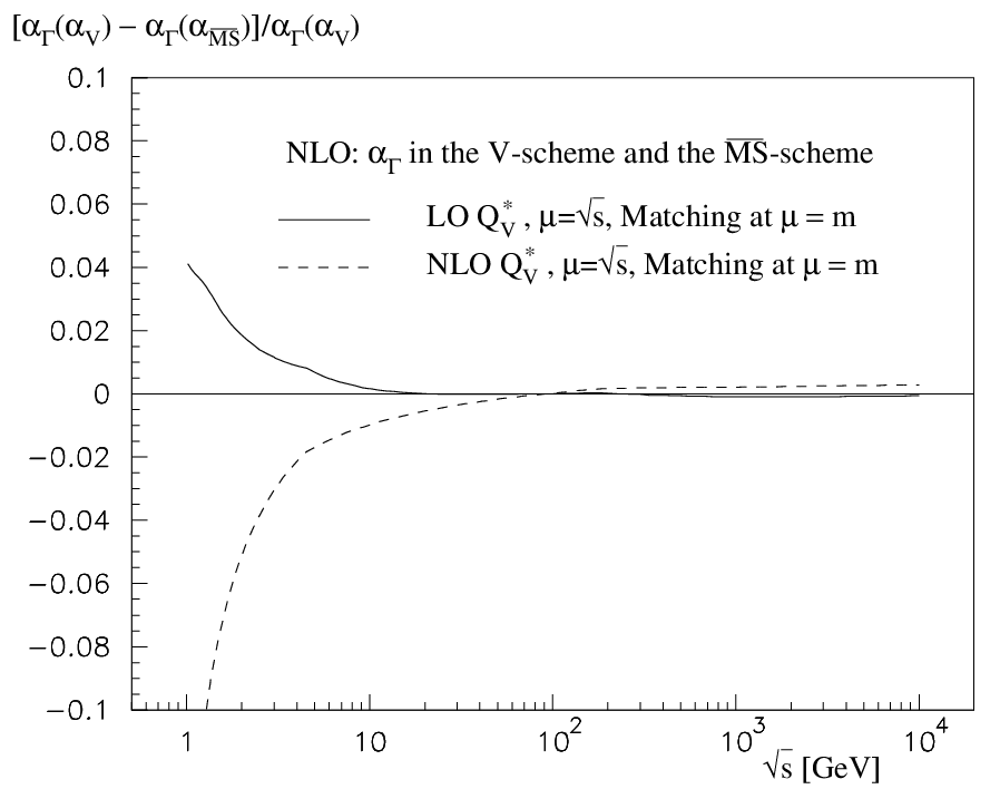
The comparison shown in Fig. 6 illustrates the relative difference between the predictions for $\alpha_{\Gamma}^{NS}(\sqrt{s})$ in the $\overline{\mbox{MS}}$ and V schemes. It has been shown[38] that the different ways of including the finite quark mass effects is smaller than $\sim 0.1\%$ by comparing the $\overline{\mbox{MS}}$ scheme with the analytic extension of the same which properly takes into account the flavor threshold effects analytically. Therefore the difference between the $\overline{\mbox{MS}}$ and V scheme predictions for $\alpha_{\Gamma}^{NS}(\sqrt{s})$ can be attributed to the scheme dependence. This is illustrated by the fact that when using the next-to-leading order approximation for the commensurate scale, instead of the leading order one, the relative difference changes sign and even becomes larger. This sensitivity is a consequence of the scale dependence of the coupling, especially at small scales where the $\Psi$-function is large. The proper inclusion of the finite quark mass effects is verified by the smoothness of the curve.

The observation of rapidly increasing structure functions in deep inelastic scattering at small-$x_{bj}$ and the observation of rapidly increasing diffractive processes such as $\gamma^{*}p\to\rho p$ at high energies at HERA is in agreement with the expectations of the BFKL[46] QCD high-energy limit. The highest eigenvalue, $\omega^{\max}$, of the LO BFKL equation[46] is related to the intercept of the Pomeron which in turn governs the high-energy asymptotics of the cross sections: $\sigma\sim s^{\alpha_{I\negthinspace P}-1}=s^{\omega^{\max}}$. The BFKL Pomeron intercept in LO turns out to be rather large: $\alpha_{I\negthinspace P}-1=\omega_{L}^{\max}=12\,\ln 2\,(\alpha_{S}/\pi)\simeq 0.55$ for $\alpha_{S}=0.2$; hence, it is very important to know the NLO corrections.

Recently the NLO corrections to the BFKL resummation of energy logarithms were calculated[47, 48] by employing the $\overline{\mbox{MS}}$ scheme to regulate the ultraviolet divergences with arbitrary scale setting. The NLO corrections to the highest eigenvalue of the BFKL equation turn out to be negative and even larger than the LO contribution for $\alpha_{s}>0.157$. It is thus important to analyze the NLO BFKL resummation of energy logarithms in physical renormalization schemes and apply the BLM-CSR method. In fact, as shown in a recent paper,[49] the reliability of QCD predictions for the intercept of the BFKL Pomeron at NLO when evaluated using BLM scale setting[6] within non-Abelian physical schemes, such as the momentum space subtraction (MOM) scheme[50, 51] or the $\Upsilon$-scheme based on $\Upsilon\rightarrow ggg$ decay, is significantly improved compared to the $\overline{\mbox{MS}}$-scheme.

The renormalization scale ambiguity problem can be resolved if one can optimize the choice of scales and renormalization schemes according to some sensible criteria. In the BLM optimal scale setting,[6] the renormalization scales are chosen such that all effects related to the QCD $\beta$-function are resummed into the running couplings. The coefficients of the perturbative series are thus identical to the perturbative coefficients of the corresponding conformally invariant theory with $\beta=0$.

In the present case one can show that within the V-scheme (or the $\overline{\mbox{MS}}$-scheme) the BLM procedure does not change significantly the value of the NLO coefficient $r(\nu)$. This can be understood since the V-scheme, as well as $\overline{\mbox{MS}}$-scheme, are adjusted primarily to the case when in the LO there are dominant QED (Abelian) type contributions, whereas in the BFKL case there are important LO gluon-gluon (non-Abelian) interactions. Thus one can choose for the BFKL case the MOM-scheme[50, 51] or the $\Upsilon$-scheme based on $\Upsilon\rightarrow ggg$ decay.

Adopting BLM scale setting, the NLO BFKL eigenvalue in the MOM-scheme is

where $r_{BLM}^{MOM}(\nu)$ is given numerically in Table 1 and the BLM scale is given by,

where $I=-2\int^{1}_{0}dx\,{\rm ln}(x)/[x^{2}-x+1]\sim 2.3439$. At $\nu=0$ we have $Q^{MOM\,2}_{BLM}(0)=Q^{2}\bigl(4\exp[2(1+2I/3)-5/3]\bigr)\simeq Q^{2}\,127$. Note that $Q^{MOM\,2}_{BLM}(\nu)$ contains a large factor, $\exp[2(1+2I/3)]\simeq 168$, which reflects a large kinematic difference between MOM- and $\overline{\mbox{MS}}$- schemes.[52, 6]

Figure 7 gives the result for the $Q^{2}$ dependence of the eigenvalue of the NLO BFKL kernel using the QCD parameter $\Lambda=0.1$ GeV which corresponds to $\alpha_{S}=4\pi/\bigl[\beta_{0}\ln(Q^{2}/\Lambda^{2})\bigr]\simeq 0.2$ at $Q^{2}=15$ GeV².

One of the striking features of this analysis is that the NLO value for the intercept of the BFKL Pomeron, improved by the BLM procedure, has a very weak dependence on the gluon virtuality $Q^{2}$. This agrees with the conventional Regge-theory where one expects an universal intercept of the Pomeron without any $Q^{2}$-dependence. The minor $Q^{2}$-dependence obtained, on one side, provides near insensitivity of the results to the precise value of $\Lambda$, and, on the other side, leads to approximate scale and conformal invariance. Thus one may use conformal symmetry[53, 54] for the continuation of the present results to the case $t\neq 0$.

The NLO corrections to the BFKL equation for the QCD Pomeron thus become controllable and meaningful provided one uses physical renormalization scales and schemes relevant to non-Abelian gauge theory. BLM scale setting automatically sets the appropriate physical renormalization scale by absorbing the non-conformal $\beta$-dependent coefficients. These results open new windows for applications of NLO BFKL resummation to high-energy phenomenology. and constitutes a first step towards a more complete understanding of the NLO corrections to the structure functions in the Regge limit. An important issue raised by R. Thorne[55] is the factorization scheme dependence of the result. Ideally one should make the analysis employing a physical factorization scheme.[3, 56]

Recently the $L3$ collaboration at LEP has presented new results for the virtual photon cross section $\sigma(\gamma^{*}(Q_{A})\gamma^{*}(Q_{b})\to{\rm hadrons})$ using double tagged $e^{+}e^{-}\to e^{+}e^{-}{\rm hadrons}.$ This process provides a remarkably clean possible test of the perturbative QCD pomeron since there are no initial hadrons.[57] The calculation of $\sigma(\gamma^{*}\gamma^{*})$ is discussed in detail in references.[57] We note here some important features:

i) For large virtualities, $\sigma(\gamma^{*}\gamma^{*})$ the longitudinal cross section $\sigma_{LL}$ dominates and scales like $1/Q^{2}$, where $Q^{2}\sim{\mbox{\rm max}}\{Q_{A}^{2},Q_{B}^{2}\}$. This is characteristic of the perturbative QCD prediction. Models based on Regge factorization (which work well in the soft-interaction regime dominating $\gamma\,\gamma$ scattering near the mass shell) would predict a higher power in $1/Q$.

ii) $\sigma(\gamma^{*}\gamma^{*})$ is affected by logarithmic corrections in the energy $s$ to all orders in $\alpha_{s}$. As a result of the BFKL summation of these contributions, the cross section rises like a power in $s$, $\sigma\propto s^{\lambda}$. The Born approximation to this result; that is, the ${\cal O}(\alpha_{s}^{2})$ contribution, corresponding to single gluon exchange gives a constant cross section, $\sigma_{\rm Born}\propto s^{0}$. A fit to photon-photon sub-energy dependence measured by L3 at $\sqrt{s}_{e^{+}e^{-}}=91~{\rm GeV}$ and $\left\langle{Q_{A}^{2}}\right\rangle=\left\langle{Q_{B}^{2}}\right\rangle=3.5~{\rm GeV}^{2}$ gives $\alpha_{P}-1=0.28\pm 0.05$. The L3 data at $\sqrt{s}_{e^{+}e^{-}}=183~{\rm GeV}$ and $\left\langle{Q_{A}^{2}}\right\rangle=\left\langle{Q_{B}^{2}}\right\rangle=14~{\rm GeV}^{2},$ gives $\alpha_{P}-1=0.40\pm 0.07$ which shows a rise of the virtual photon cross section much stronger than single gluon or soft pomeron exchange, but it is compatible with the expectations from the NLO scale- and scheme-fixed BFKL predictions. It will be crucial to measure the $Q_{A}^{2}$ and $Q_{B}^{2}$ scaling and polarization dependence and compare with the detailed predictions of PQCD.[57]

References

- 1 . S.J. Brodsky, H.J. Lu, Phys. Rev. D51, 3652 (1995); hep-ph/9506322.
- 2 . S. J. Brodsky , G. T. Gabadadze, A. L. Kataev, and H. J. Lu. Phys. Lett. B 372, 133 (1996).
- 3 . G. Grunberg, Phys. Lett. B85. 70 (1980); Phys. Lett. B110, 501 (1982); Phys. Rev. D29, 2315 (1984).
- 4 . A. Dhar and V. Gupta, Phys. Rev. D29, 2822 (1984).
- 5 . V. Gupta, D. V. Shirkov and O. V. Tarasov, Int. J. Mod. Phys. A6, 3381 (1991).
- 6 . S. J. Brodsky, G. P. Lepage and P. B. Mackenzie, Phys. Rev. D28, 228 (1983).
- 7 . G. ’t Hooft, in the Proceedings of the International School, Erice, Italy, 1977, edited by A. Zichichi, Subnuclear Series Vol. 15 (Plenum, New York, 1979).
- 8 . A. H. Mueller, Phys. Lett. B308, 355 (1993).
- 9 . H. J. Lu, Phys. Rev. D45, 1217 (1992).
- 10 . M. Beneke and V. M. Braun, Phys. Lett. B348, 513 (1995).
- 11 . S. J. Brodsky and P. Huet, Phys. Lett. B417, 145 (1998).
- 12 . G. Peter Lepage and P. B. Mackenzie, Phys. Rev. D48, 2250 (1993).
- 13 . M. Neubert, Phys. Rev. D51, 5924 (1995).
- 14 . P. Ball, M. Beneke and V. M. Braun, Nucl. Phys. B452, 563 (1995).
- 15 . S.J. Brodsky, M. Melles, J. Rathsman, SLAC–PUB–8019, hep-ph/9906324.
- 16 . A. Czarnecki, K. Melnikov, and N. Uraltsev, Phys. Rev. Lett. 80, 3189 (1998). Yu. L. Dokshitser and B. R. Webber, Phys. Lett. B404, 321 (1997).
- 17 . S. Adler, Phys. Rev. 182, 1517 (1969).
- 18 . A. C. Mattingly and P. M. Stevenson, Phys. Rev. D49, 437 (1994).
- 19 . CCFR Collaboration, W.C. Leung, et al., Phys. Lett. B317, 655 (1993).
- 20 . CCFR and NuTeV Collaboration, presented by D. Harris at XXX Recontre de Moriond, 1995, presented by J. H. Kim at the European Conference on High Energy Physics, Brussels, July 1995.
- 21 . A. L. Kataev, A.V. Sidorov, Phys. Lett. B331, 179 (1994).
- 22 . CCFR Collaboration, P.Z. Quinta, et al., Phys. Rev. Lett. 71, 1307 (1993).
- 23 . A. De Rújula and H. Georgi, Phys. Rev. D13, 1296 (1976).
- 24 . H. Georgi and H.D. Politzer, Phys. Rev. D14, 1829 (1976).
- 25 . D.A. Ross, Nucl. Phys. B140, 1 (1978); T. Goldman and D.A. Ross, Nucl. Phys. B171, 273 (1980).
- 26 . D. V. Shirkov, Teor. Mat. Fiz. 98, 500 (1992) [Theor. Math. Phys. 93, 1403 (1992)]; D. V. Shirkov and S. V. Mikhailov, Zeit. Phys. C63, 463 (1994).
- 27 . J. Chýla, Phys. Lett. B 351, 325 (1995).
- 28 . T. Yoshino, K. Hagiwara, Z.Phys. C 24, 185 (1984).
- 29 . F. Jegerlehner, O.V. Tarasov, hep-ph/9809485 and DESY 98-093.
- 30 . T. Appelquist, J. Carazzone, Phys. Rev. D11, 2856 (1975).
- 31 . M. Melles, hep-ph/9805216, Phys. Rev. D58:114004, 1998.
- 32 . C.T.H. Davies, et al., Phys. Lett. B345, 42 (1995); Phys. Rev. D56, 2755 (1997).
- 33 . S. J. Brodsky, C.-R. Ji, A. Peng and D. G. Robertson, Phys. Rev. D57, 345 (1998).
- 34 . A. Szczepaniak, E. M. Henley, S. J. Brodsky, Phys. Lett. B243, 287 (1990).
- 35 . B. H. Smith, M. B. Voloshin, Phys. Lett. B324, 117 (1994). Erratum-ibid. B333, 564 (1994).
- 36 . S.J. Brodsky, A. H. Hoang, J. H. Kuhn, and T. Teubner, Phys. Lett. B359, 355 (1995).
- 37 . V. S. Fadin, V. A. Khoze, A. D. Martin, and W. J. Stirling, Phys. Lett. B363, 112 (1995).
- 38 . S. J. Brodsky, M. S. Gill, M. Melles, and J. Rathsman, Phys. Rev. D58, 116006 (1998).
- 39 . P. N. Burrows, Acta Phys. Polon. B28, 701 (1997).
- 40 . S. J. Brodsky, Y. Frishman and G. P. Lepage, Phys. Lett. 167B, 347 (1986); S. J. Brodsky, P. Damgaard, Y. Frishman and G. P. Lepage, Phys. Rev. D33, 1881 (1986).
- 41 . D. Muller, Phys. Rev. D59, 116001 (1999); A. V. Belitsky and D. Muller, Nucl. Phys. B537, 397 (1999); D. Muller, Phys. Rev. D49, 2525 (1994).
- 42 . J. Blümlein, V. Ravindran and W. L. van Neerven, Acta Phys. Polon. B29, 2581 (1998).
- 43 . K.G. Chetyrkin, Phys. Lett. B 307, 169 (1993).
- 44 . D.E. Soper and L.R. Surguladze, Phys. Rev. Lett. 73, 2958 (1994).
- 45 . S.A. Larin, T. van Ritbergen, J.A.M. Vermaseren, Nucl. Phys. B438, 278 (1995).
- 46 . V. S. Fadin, E. A. Kuraev and L. N. Lipatov, Phys. Lett. 60B, 50 (1975); L. N. Lipatov, Yad. Fiz. 23, 642 (1976) [Sov. J. Nucl. Phys. 23, 338 (1976)]; E. A. Kuraev, L. N. Lipatov and V. S. Fadin, Zh. Eksp. Teor. Fiz. 71, 840 (1976) [Sov. JETP 44, 443 (1976)]; ibid. 72, 377 (1977) [45, 199 (1977)]; Ya. Ya. Balitskiǐ and L. N. Lipatov, Yad. Fiz. 28, 1597 (1978) [Sov. J. Nucl. Phys. 28, 822 (1978)].
- 47 . V. S. Fadin and L. N. Lipatov, Phys. Lett. 429B, 127 (1998).
- 48 . G. Camici and M. Ciafaloni, Phys. Lett. 430B, 349 (1998).
- 49 . S.J. Brodsky, V.S. Fadin, V.T. Kim, L.N. Lipatov and G.B. Pivovarov, hep-ph/9901229.
- 50 .
W. Celmaster and R. J. Gonsalves,
Phys. Rev. D20, 1420 (1979);
Phys. Rev. Lett. 42, 1435 (1979). - 51 . P. Pascual and R. Tarrach, Nucl. Phys. B174, 123 (1980); (E) B181, 546 (1981).
- 52 . W. Celmaster and P. M. Stevenson, Phys. Lett. 125B, 493 (1983).
- 53 . L. N. Lipatov, Phys. Rept. C286, 131 (1997).
- 54 . L. N. Lipatov, Zh. Eksp. Teor. Fiz. 90, 1536 (1986) [Sov. JETP 63, 904 (1986)]; in Perturbative Quantum Chromodynamics, ed. A.H. Mueller (World Scientific, Singapore, 1989) p. 411; R. Kirschner and L. Lipatov, Zeit. Phys. C45, 477 (1990).
- 55 .
R.S. Thorne,
“NLO BFKL equation, running coupling and renormalization scales,”
hep-ph/9901331;
J.R. Forshaw, G.P. Salam and R.S. Thorne, “BFKL at next-to-leading order,” hep-ph/9812304. - 56 . S. Catani, “Physical anomalous dimensions at small x,” Z. Phys. C75, 665 (1997)
- 57 . S. J. Brodsky, F. Hautmann and D. E. Soper,‘ Phys. Rev. D56, 6957 (1997); S. J. Brodsky, F. Hautmann and D. E. Soper, Phys. Rev. Lett. 78, 803 (1997); F. Hautmann, talk at ICHEP96 (Warsaw, July 1996), preprint OITS 613/96, in Proceedings of the XXVIII International Conference on High Energy Physics, eds. Z. Ajduk and A. K. Wroblewski, World Scientific, p.705; J. Bartels, A. De Roeck and H. Lotter, Phys. Lett. B389, 742 (1996).
- 58 . S. J. Brodsky, J. R. Pelaez, and N. Toumbas, hep-ph/9810424, to be published in Phys. Rev. D.