Lattice calculation of $\alpha_{s}$ in momentum scheme

The conventional two-loop $\Lambda^{(c)}$ is obtained in any scheme from $\alpha(\mu^{2})\equiv g_{R}(\mu^{2})^{2}/(4\pi)$ by

$$\Lambda^{(c)}\equiv\mu\exp\left(\frac{-2\pi}{\beta_{0}\alpha(\mu^{2})}\right)\times\left(\frac{\beta_{0}\alpha(\mu^{2})}{4\pi}\right)^{-\frac{\beta_{1}}{\beta_{0}^{2}}}$$

(10)

where

$$\mu\frac{\partial\alpha}{\partial\mu}=-\frac{\beta_{0}}{2\pi}\alpha^{2}-\frac{\beta_{1}}{4\pi^{2}}\alpha^{3}-\frac{\beta_{2}}{64\pi^{3}}\alpha^{4}-...$$

(11)

$\beta_{0}=11$, $\beta_{1}=51$ and $\beta_{2}$ is scheme dependent ($\beta_{2,\overline{\rm MS}}=2857$). Integrating exactly eq. (11) expanded up to order $\alpha^{n+1}$, and imposing the asymptotic limit $\Lambda^{(n)}/\Lambda^{(c)}(\alpha)\to 1$ when $\alpha\to 0$, leads to the definition

$$\Lambda^{(2)}\equiv\left(1+\frac{\beta_{1}\alpha}{2\pi\beta_{0}}\right)^{\left(\frac{\beta_{1}}{\beta_{0}^{2}}\right)}\Lambda^{(c)}(\alpha)$$

(12)

at two loop and to the three loop $\Lambda^{(3)}$:

$$\Lambda^{(3)}\equiv\Lambda^{(c)}(\alpha)\left(1+\frac{\beta_{1}\alpha}{2\pi\beta_{0}}+\frac{\beta_{2}\alpha^{2}}{32\pi^{2}\beta_{0}}\right)^{\frac{\beta_{1}}{2\beta_{0}^{2}}}\times$$

$$\exp\left\{\frac{\beta_{0}\beta_{2}-4\beta_{1}^{2}}{2\beta_{0}^{2}\sqrt{\Delta}}\left[\arctan\left(\frac{\sqrt{\Delta}}{2\beta_{1}+\beta_{2}\alpha/4\pi}\right)-\arctan\left(\frac{\sqrt{\Delta}}{2\beta_{1}}\right)\right]\right\}$$

(13)

when $\Delta\equiv 2\beta_{0}\beta_{2}-4\beta_{1}^{2}>0$.

One simple criterium has been proposed in [6] to exhibit perturbative scaling: when plotting (10) as a function of $\mu$ perturbative scaling implies that $\Lambda$ should become constant for large enough $\mu$. We will thus try to fit each of the formulae (10), (12), (13), expressed in terms of our measured $\alpha(\mu)$, as a constant. All these formulae converge to the same $\Lambda$ when $\alpha\to 0$. But since our fits are for $\alpha$ in the range of 0.3 - 0.5, and since they do not have the same dependence on $\alpha$ they should not all fit our data. However, as we shall see, within our errors, acceptable fits are possible with (10), and (13) varying $\beta_{2}$ on a wide range. This is due to the fact that, even with our rather large statistics, the three loop effect, being only logarithmic, does not modify strongly enough the variation of $\Lambda(\alpha)$ in our fitting range although the resulting fitted $\Lambda$ depends significantly on the formula used and on $\beta_{2}$. In other words we have different acceptable fits, with slightly different slopes in $\mu$, which lead asymptotically, when $\alpha\to 0$, to significantly different $\Lambda$’s. There results a systematic error which cannot be fully eliminated until $\beta_{2}$ is really computed.

Notwithstanding this problem, we believe that the possibility to fit several of these formulae by a constant on a large range of $\mu$ and with small statistical errors, is an indication that perturbative scaling has been reached. In other words, our data show that the uncertainty is of logarithmic type (higher loops), but there is no room for significant power corrections. To study power corrections, one has to consider with care lower scales [12], and we plan to do that in a forthcoming publication [14].

In order to compare different schemes, it is standard to translate the results into the $\overline{\rm MS}$ scheme. Once known in any scheme, a one loop computation is enough to yield $\Lambda_{\rm QCD}$ in any other scheme [10], [11]. From [10] and [6] we get for zero flavors

$$\Lambda_{\rm MOM}=3.334\Lambda_{\overline{\rm MS}},\qquad\Lambda_{\widetilde{\rm MOM}}=\exp(70/66)\simeq 2.888\Lambda_{\overline{\rm MS}}.$$

(14)

In a finite hypercubic volume the momenta are the discrete set of vectors

$$p_{\mu}=2\pi n_{\mu}/L$$

(15)

where $n_{\mu}$ are integer and $L$ is the lattice size. The isometry group for momenta is generated by the four reflections $p_{\mu}\to-p_{\mu}$ for $\mu=1,\cdots,4$ and the permutations between the four directions such as $p_{x}\leftrightarrow p_{y}$. Altogether this group has $2^{4}\,4!=384$ elements. We use fully this symmetry in order to increase the statistics. The functions $G^{(2)}(p^{2})$ and $G^{(3)}(p^{2},0,p^{2})$ in eqs (1) and (7) are systematically symmetrized over the momenta lying on one given group orbit. The number of distinct momenta in an orbit is 384 or a divisor of 384 (when the momentum is invariant by some subgroup).

In the case of $G^{(3)}(p^{2},p^{2},p^{2})$ in eq. (5) we furthermore symmetrize over the 6 permutations of external legs (Bose symmetry). The number of elements in an orbit will be $6\times 384=2304$ or one of its divisors.

We build all triplets of momenta up to some maximum value of the momentum to be specified later.

In the asymmetric case, there are as many triplets as momenta. For every integer number there exists at least one orbit of the isometry group with $n_{\mu}n^{\mu}$ equal to that integer. The number of elements is often a much smaller number than 384: 1, 8, 16, 24, 64, etc.

In the symmetric case, $n_{\mu}n^{\mu}$ has to be an even number: $n_{1}^{2}=n_{2}^{2}=(n_{1}+n_{2})^{2}$, where the subindices label the external particles, and consequently, $n_{1\mu}n_{2}^{\mu}=-n_{1}^{2}/2$ being an integer, $n_{1}^{2}$ is even. It happens that for every even integer, we have found at least one orbit. The number of elements in one orbit is often a large number, 2304 and 1152 are frequent, 576 and 192 are less. Notwithstanding these larger sets, the statistical noise will turn out to be larger in the symmetric case than in the asymmetric one. Let us give some examples of symmetric triplets: for $n^{2}=2$: $(1100)(0-110)(-10-10)$ and its 192 tranformed by the isometry-Bose group; for $n^{2}=4$: $(2000)(-1111)(-1-1-1-1)$ and its 192 transformed. For $n^{2}=16$: $(4000)(-2222)(-2-2-2-2)$ its 192 transformed. For $n^{2}=18$ there are 6 orbits, for example $(4110)(-1-2-32)(-312-2)$ and its 2304 transformed, $(3300)(-1-232)(-2-1-3-2)$ and its 1152 transformed, etc.

The calculation has been performed on a QUADRICS QH1, with hypercubic lattices of $16^{4}$ and $24^{4}$ sites at $\beta=6.0$, $24^{4}$ at $\beta=6.2$ ( all three with 1000 configurations) and $32^{4}$ at $\beta=6.4$ (100 configurations), combining the Metropolis and the overrelaxation algorithms.

The configurations have been transformed to the Landau gauge by a combination of overrelaxation algorithm and Fourier acceleration. We end when $|\partial_{\mu}A_{\mu}|^{2}<10^{-12}$ and when the spatial integral of $A_{0}$ is constant in time to better than $10^{-5}$.

We define

$$A_{\mu}(x+\hat{\mu}/2)=\frac{U_{\mu}(x)-U_{\mu}^{\dagger}(x)}{2iag_{0}}-\frac{1}{3}\hbox{Tr}\left(\frac{U_{\mu}(x)-U_{\mu}^{\dagger}(x)}{2iag_{0}}\right)$$

(16)

where $\hat{\mu}$ indicates the unit lattice vector in the direction $\mu$ and $g_{0}$ is the bare coupling constant, and compute the n-point Green functions in momentum space from

$$G^{(n)\,a_{1}a_{2}\cdots a_{n}}_{\mu_{1}\mu_{2}\cdots\mu_{n}}(p_{1},p_{2},\cdots p_{n})=<A_{\mu_{1}}^{a_{1}}(p_{1})A_{\mu_{2}}^{a_{2}}(p_{2})\cdots A_{\mu_{n}}^{a_{n}}(p_{n})>$$

(17)

where $p_{1}+p_{2}+..+p_{n}=0$, $<>$ indicates the Monte-Carlo average and where

$$A_{\mu}^{a}(p)=\frac{1}{2}\hbox{Tr}\left[\sum_{x}A_{\mu}(x+\hat{\mu}/2)\exp(ip(x+\hat{\mu}/2))\lambda^{a}\right]$$

(18)

$\lambda^{a}$ being the Gell-Mann matrices and the trace being taken in the $3\times 3$ color space.

We have computed the Fourier transforms up to a maximum momentum of $\simeq 3$ GeV at $\beta=6$, and $\simeq 4.2$ GeV at $\beta=6.2$ and $\beta=6.4$. These maxima correspond to $n^{2}\equiv n_{\mu}n^{\mu}\leq 16$ for $(\beta,V)=(6.0,16^{4})$ and $\leq 36$ for all the other cases.

From the color structure of QCD we expect the two point Green functions to be proportional to the color tensor $\delta_{a_{1}a_{2}}$. This is indeed the case to an accuracy of the order of 1 %. Furthermore one can prove from gauge symmetry (global and local) and Bose symmetry that the three point Green functions have to be proportional to $f^{a_{1}a_{2}a_{3}}$ in the MOM and $\widetilde{\rm MOM}$ schemes. This is indeed the case, but the errors now depend on the momentum. For small values of $n^{2}$ the agreement is of a few percent. The errors increase with $n^{2}$ and when $n^{2}$ reaches the $30$’s the error reaches 100 %. This is an indication that the large momenta are grieved by noise. Luckily this caution is necessary only for the very few largest values of $n^{2}$ that we have considered. Indeed we will exclude the points $n^{2}>30$ from our fits. In order to reduce the noise we work from now on with color averaged Green functions: $\frac{1}{24}G^{(3)\,a_{1}a_{2}a_{3}}f^{a_{1}a_{2}a_{3}}$ and $\frac{1}{8}G^{(2)\,a_{1}a_{2}}\delta_{a_{1}a_{2}}$.

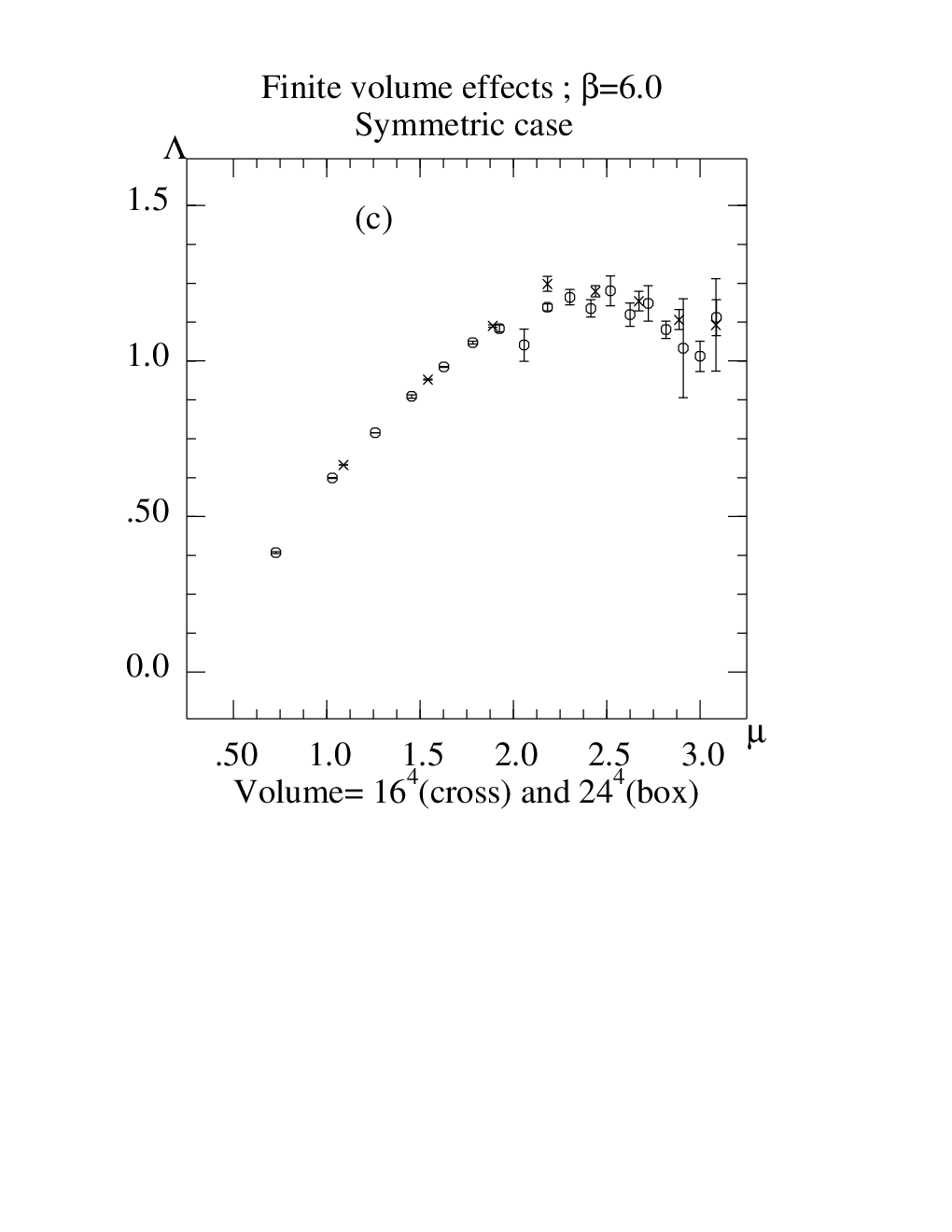
The finite volume effects can be checked by a comparison of the two calculations at $\beta=6.0$, Fig 1. For relatively small $\mu$, close to the maximum of $\alpha$, there is a visible decrease of $\alpha$ when the volume is increased.

For larger $\mu$, the volume dependence is still visible, but reduced to a few percent. Comparing the values of $\Lambda$ fitted in the asymptotic region given in table 1, one finds

$$\Lambda_{sym}(24)/\Lambda_{sym}(16)=0.96\pm 0.02,\qquad\Lambda_{asym}(24)/\Lambda_{asym}(16)=0.97\pm 0.02$$

(19)

which indicates that the finite volume effect affects moderately the asymptotic estimate of $\Lambda$. More study is needed to quantify precisely this effect. Still, from gross estimates, our largest physical volume, $\beta=6.0,\,24^{4}$, lies presumably within 5% above the infinite volume limit.

Figs. 1(a,b) show the shape of $\alpha(\mu)$. The same shape is seen for the other $\beta$’s. In fact $\alpha(\mu)$ scales in $a$ to a very good accuracy. We keep this study for another publication [14].

Turning to the scaling in $\mu$, we see from figs 1(c,d) that both $\Lambda$’s do not really show plateaus at large momentum: they go through a maximum around 2 GeV and fall down later on. Our study shows that this feature cannot be cured simply by a three loop effect. Using eq. (13) with different values for $\beta_{2}$ cannot lead to acceptable plateaus for all lattice spacings. Since the fall at large $\mu$ is observed systematically, beyond statistical errors, but decreases when $\beta$ increases, we conjecture that we deal with an $O(a^{2}p^{2})$ effect.

We have successfully tried a correction which will be described now. It starts from the remark that in the lattice Landau gauge, obtained by minimizing $\sum_{\mu,x}{\rm Tr}[1-U_{\mu}(x)]$, $p_{\mu}A^{a}_{\mu}(p)$ does not vanish while $\tilde{p}_{\mu}A^{a}_{\mu}(p)$ does, when $A_{\mu}^{a}(p)$ is defined from eq (18) and where

$$\tilde{p}_{\mu}=\frac{2}{a}\sin\left(\frac{ap_{\mu}}{2}\right).$$

(20)

The latter momentum differs from the one in (15) by $O(a^{2}p^{2})$: $\tilde{p}_{\mu}\simeq p_{\mu}(1-\frac{1}{24}a^{2}p_{\mu}^{2})$. It results that the lattice two point Green function is not really proportional to the tensor in (1) but to the tensor deduced from (1) with $p_{\mu}$ substituted by $\tilde{p}_{\mu}$, [9].

We perform a similar change in the tensors used to extract $\alpha$. The projectors in (6) and (8) have been normalized to give 1 when contracted to the tensors which multiply $G^{(3)}$ in (5) and (7) respectively. Assuming that the lattice calculations is such as to produce the tensors in (5) and (7) with $p_{\mu}$ substituted by $\tilde{p}_{\mu}$, there would be a bias in our formulae (6) and (8). Indeed the contraction of the “tilded” tensors in (5) and (7) with the tensors in (6) and (8) is smaller than one and decreases with increasing $p$. We tentatively correct the bias by dividing the result in (3) by this factor smaller than one. We shall refer to this as the “sinus improvement”.

For brevity we only show $(\beta,V)=(6.2,\,24^{4})$ in fig. 2. The improvement of the plateaus is dramatic. The large $\mu$ fall has been considerably reduced. The improvement is confirmed by a reduction of the $\chi^{2}$ per degree of freedom from exceedingly large values to acceptable ones, see tables 2 and 3.

Of course, this is only an ad hoc $O(a^{2}p^{2})$ improvement, by no way rigorous and systematic. Fitting directly a corrective term of the form $1-ca^{2}p^{2}$ leads also to drastically improved $\chi^{2}$ with best values of $c$ in reasonable agreement with the “sinus improvement” ($c\sim 1/24$). It should be stressed that the sinus improvement, and the $1-ca^{2}p^{2}$ fits yield very similar values of $\Lambda$. We may thus conclude that the $O(a^{2}p^{2})$ systematic error on $\Lambda$ is moderate after “sinus improvement”.

A final source of systematic uncertainty comes from our ignorance of $\beta_{2}$ in the MOM scheme. From a preliminary perturbative calculation [15] in the $\widetilde{\rm MOM}$ scheme we get $\beta_{2}\simeq 4824$. On the other hand we unsuccessfully tried to fix $\beta_{2}$ non-perturbatively from our asymptotic fits. The ratio $\Lambda^{(3)}/\Lambda^{(c)}$, eqs (10)-(13), drops from 1 when $\alpha$ increases, the drop increasing with $\beta_{2}$. As a result, the fitted value for $\Lambda^{(3)}$ will decrease as $\beta_{2}$ increases. Simultaneously the shape of the plateaus are modified. In principle, the requirement of an acceptable $\chi^{2}$ might have restricted the admissible domain for $\beta_{2}$. Unhappily our preliminary analysis did not turn out to be so restrictive. Only for $\beta_{2}$ below $0.5\,\beta_{2,\overline{\rm MS}}$ does the $\chi^{2}$ become prohibitive, see for example the $\beta_{2}=0$ case ($\Lambda^{(2)}$) in tables 2 and 3. It might look strange that $\Lambda^{(c)}$ fits well while $\Lambda^{(2)}$ does not, both being two-loop formulae. In fact $\Lambda^{(c)}$ is only an approximate two-loop formula which can be proven to be very close to $\Lambda^{(3)}$ with $\beta_{2}\simeq 8\frac{\beta_{1}^{2}}{\beta_{0}}\simeq 0.66\beta_{2,\overline{\rm MS}}$.

We therefore cannot do better in the MOM scheme, at present, than to provide fits of $\Lambda^{(3)}$ as a function of $\beta_{2}$. For comparison we also provide the same analysis in the $\widetilde{\rm MOM}$ scheme. The maximum value for $\beta_{2}$ which we consider is $\beta_{2}=2\beta_{2,\overline{\rm MS}}=5714$ since, for such a large value, the term $\propto\alpha^{4}$ in the $\beta$ function (11) is of the same order as the term $\propto\alpha^{3}$ for our range of $\alpha$. If $\beta_{2}$ was larger than that, the perturbative expansion would be dubious, and the evidence for perturbative scaling shown by our data would appear as a miraculous fake.

The “sinus improved” $\Lambda$’s exhibit a very clear scaling when $\mu$ varies above 2.1 GeV, as can be seen from the quality of the plateaus in figs 2 and 3 and from the $\chi^{2}$ per d.o.f. In this subsection we want to study further the scaling when $\beta$, i.e. $a$, is varied.

Since $\Lambda$ depends linearly on $a^{-1}$, the consistency of our fits can only be checked through a spacing independent ratio. We use the ratios $a\Lambda/(a\sqrt{\sigma})$, see table 1, where $a\sqrt{\sigma}$ is the central value of string tension computed in [2].

In order to write $\Lambda$ in physical units we then multiply all ratios by one global scale factor: $\sqrt{\sigma}_{0}=445$ MeV tuned to the central value of a very recent fit [13] from the $K^{\ast}$ mass: $a^{-1}{(\beta=6.2)}=2.75(18)$ GeV. We take the central value: $a^{-1}{(\beta=6.2)}=2.75$ GeV, whence $a^{-1}{(\beta=6.0)}=1.966$ GeV and $a^{-1}{(\beta=6.4)}=3.664$ GeV.

This leads to the plots in fig. 3. The presence of nice plateaus is striking. We fit the average $\Lambda$ on these plateaus, for scales never smaller than 2.1 GeV, and as high as allowed by lattice effects. The results are presented in tables 1, 2 and 3. The fits for $\Lambda^{(c)}$ and for a large range of $\Lambda^{(3)}$ yield a $\chi^{2}$ per degree of freedom smaller than 1.5. Scaling in the lattice spacing is striking, especially for those lattice parameters which correspond to a similar physical volume of $\simeq(1.7\,{\rm fm})^{4}$, i.e. $(\beta,V)=(6.0,\,16^{4}),(6.2,\,24^{4})$ and $(6.4,\,32^{4})$. They average to:

$$\Lambda^{(c)}_{\overline{\rm MS}}=378(6)\,{\rm MeV}\ ({\rm symmetric})\qquad\Lambda^{(c)}_{\overline{\rm MS}}=355(4)\,{\rm MeV}\ ({\rm asymmetric})$$

$$\Lambda^{(3)}_{\overline{\rm MS}}\left(\beta_{2}=1.69\,\beta_{2\,\overline{\rm MS}}=4824\right)\,=\,\left\{\matrix{327(5)\,{\rm MeV}\ ({\rm symmetric})\cr 313(3)\,{\rm MeV}\ ({\rm asymmetric})\cr}\right.$$

(21)

where the errors are only statistical. $\beta_{2}=4824$ results from our preliminary calculation [15] in the asymmetric scheme. For comparison we provide the result with the same $\beta_{2}$ in the symmetric case. The result at the larger volume of $\simeq(2.44\,{\rm fm})^{4}$, $(\beta,V)=(6.0,24^{4})$, presumably close to the infinite volume limit (section 2.3), is:

$$\Lambda^{(c)}_{\overline{\rm MS}}=361(6)\,{\rm MeV}\ ({\rm symmetric})\qquad\Lambda^{(c)}_{\overline{\rm MS}}=345(6)\,{\rm MeV}\ ({\rm asymmetric})$$

$$\Lambda^{(3)}_{\overline{\rm MS}}\left(\beta_{2}=1.69\,\beta_{2\,\overline{\rm MS}}=4824\right)\,=\left\{\matrix{\,311(5)\,{\rm MeV}\ ({\rm symmetric})\cr 303(5)\,{\rm MeV}\ ({\rm asymmetric})\cr}\right.$$

(22)

Varying $\beta_{2}$ we find acceptable $\chi^{2}$’s from $\beta_{2}\approx 0.5\beta_{2,\overline{\rm MS}}=1428$ up to beyond $2\beta_{2,\overline{\rm MS}}=5714$ which we take as the maximum perturbatively consistent value, see section 2.5. In this range of $\beta_{2}$ the fitted $\Lambda^{(3)}$ have, to a surprisingly good approximation, a linear dependence on $\beta_{2}$. We provide the result in the next section.

Finally it is worth mentioning that we have also checked scaling of $\alpha$ in $a$ over the whole range in $\mu$, including the small values. We leave this point for a forthcoming publication [14]

References

- [1] M. Lüscher, Talk given at the 18th International Symposium on Lepton-Photon Interactions, Hamburg, 28 July-1 August 1997; Lecture at l’Ecole des Houches, August 26-29 1997; M.Lüscher, R.Sommer, P.Weisz and U. Wolf, Nucl. Phys. B413(1994)481.
- [2] G.S. Bali and K. Schilling Phys. Rev. D47 (1993) 661.
- [3] G.S.Bali, In Prodvino 1993, Problems on high energy physics and field theory 147-163, hep-lat/9311009.
- [4] G.P.Lepage and P. Mackenzie, Phys. Rev. Lett. D48(1992)2250.
- [5] G. de Divitiis et al, Nucl. Phys. B433(1995)390; B437(1995)447.
- [6] B. Alles, D. Henty, H. Panagopoulos, C. Parrinello, C. Pittori, D.G. Richards, Nucl. Phys. B502 (1997) 325; C. Parrinello Nucl. Phys. Proc. Suppl. 63 (1998) 245; B. Alles, D. Henty, H. Panagopoulos, C. Parrinello, C. Pittori, IFUP-TH-23-96, hep-lat/9605033.
- [7] H.D. Politzer, Phys. Reports 14C (1974) 141.
- [8] J.S. Ball and T-W. Chiu, Phys. Rev. D22 (1980) 2550.
- [9] D.Zwanziger, Nucl Phys. B364 (1991)127.
- [10] W.Celmaster and R.J.Gonsalves Phys. Rev. D20 (1979) 1420.
- [11] A.Billoire Phys. Lett. B104 (1981) 472.
- [12] G. Burgio, F. Di Renzo, C. Parrinello and C. Pittori, LTH 417, hep-ph/9808258.
- [13] D. Becirevic et al. LPTHE-Orsay 98/33, hep-lat/9809129.
- [14] D. Becirevic et al. in preparation.
- [15] Ph. Boucaud et al. in preparation
- [16] A.I.Davydychev, P.Osland and O.V.Tarasov Phys. Rev. D58 (1998) 036007.