1Introduction

LU TP 97–12

May 1997

Creating a hybrid of matrix elements and parton showers
Johan André
Department of Theoretical Physics,
Lund University, Lund, Sweden

Abstract
The second-order QCD matrix elements give a very good agreement with experimental data on the angular distributions of the four-jet events in $\mathrm{e}^{+}\mathrm{e}^{-}$ collisions at the $\mathrm{Z^{0}}$ resonance energy. Unfortunately the description of the sub-jet structure is quite poor. The alternative approach, parton showers, gives a good description of the sub-jet structure but is worse than matrix elements when it comes to the angular distributions. Here is presented a hybrid between the matrix elements and the parton showers that is intended to combine the best of the two approaches.

1 Introduction

According to the viewpoint of modern particle physics all matter in the universe is composed of the particles listed in the table below.

\begin{array}[]{lllll}&\underline{\mathrm{Quarks}}&&\underline{\mathrm{Leptons}}&\\ \mathrm{Charge}&\mathrm{2/3}&\mathrm{-1/3}&\mathrm{-1}&\mathrm{0}\\ \underline{\mathrm{Generation}}&&&&\\ \mathrm{first}&\mathrm{u~(5\cdot 10^{-3})}&\mathrm{d~(7\cdot 10^{-3})}&\mathrm{e~(0.5\cdot 10^{-3})}&\mathrm{\nu_{e}~(0)}\\ \mathrm{second}&\mathrm{c~(1.5)}&\mathrm{s~(0.2)}&\mathrm{\mu~(0.106)}&\mathrm{\nu_{\mu}~(0)}\\ \mathrm{third}&\mathrm{t~(170)}&\mathrm{b~(5)}&\mathrm{\tau~(1.784)}&\mathrm{\nu_{\tau}~(0)}\end{array}

(1)

The approximate particle masses in the parentheses are given in GeV. All these particles have spin 1/2 and are therefore fermions. This means that the total wave-function $\Psi(q_{1},\ldots,q_{N})$ of a $N$ particle system is antisymmetric under the permutation of two identical particles i.e. $\Psi(\ldots,q_{i}\ldots,q_{j},\ldots)=-\Psi(\ldots,q_{j}\ldots,q_{i},\ldots)$ . Thus two identical particles $i$ and $j$ can’t have identical quantum numbers $q_{i}=q_{j}$ because this would imply that $\Psi=0$ . This is the so-called Pauli principle that determines the structure of the periodic system. The particles in the second and third generations have the same properties as the corresponding particles in the first generation except for the masses that increases with the generation number. It is only the particles in the first generation that is needed to build the matter on earth.

There are four known fundamental interactions between the matter particles. These are the electromagnetic, the weak, the strong and the gravitational interactions. For the first three interactions we have quantum mechanical theories possessing local gauge symmetries, in which the forces are mediated by exchange of virtual particles. The fourth interaction, gravitation, is currently described by Einstein’s general theory of relativity, which is a classical theory. One of the main objectives of current theoretical research is to find the correct quantum mechanical description of the gravitation. Fortunately the gravitational interactions between the particles studied in particle physics experiments are so weak that they can be leaved out of account. The interactions, their mediating particles and the matter they affect are listed in the table below.

\begin{array}[]{lll}\underline{\mathrm{Interaction}}&\underline{\mathrm{Particle}}&\underline{\mathrm{Affects}}\\ \mathrm{electromagnetic}&\mathrm{\gamma}&\mathrm{all~except~\nu_{e}~,\nu_{\mu}~,\nu_{\tau}}\\ \mathrm{weak}&\mathrm{W^{+}~~W^{-}~~Z}^{0}&\mathrm{all~particles}\\ \mathrm{strong}&\mathrm{g}_{i}~~i=1\ldots 8&\mathrm{all~quarks}\\ \mathrm{gravitation}&\mathrm{graviton}&\mathrm{all~particles}\end{array}

(2)

All these particles have integer spin and are therefore bosons. The $\gamma$ particle which mediates the electro-magnetic interaction is a spin 1 particle. The virtual $\mathrm{\gamma}$ particle is massive and can therefore exist in the tree different spin-states $-1$ , $0$ and $+1$ , this corresponds to the fact that the classical $\mathrm{\vec{E}}$ and $\mathrm{\vec{B}}$ fields can be described by three independent parameters. Similar arguments lead to the conclusion that the graviton, if it exists, should be a spin 2 particle. The electromagnetic interaction is described by QED (Quantum Electro Dynamics) a theory whose predictions agrees extremely well with experimental results. This is in part due to the smallness of $\alpha=e^{2}/4\pi\varepsilon_{0}\hbar c$ in which the perturbative solutions are expanded. The weak interaction is described by a theory that combines the electromagnetic and the weak interaction into a theory of the so called electro-weak interaction. In the electro-weak theory the fundamental particles that mediate the interactions are the B, $\mathrm{W^{0}}$ , $\mathrm{W^{+}}$ and $\mathrm{W^{-}}$ particles. They are all massless, a condition that is necessary for a consistent theory. The $\mathrm{W^{+}}$ and $\mathrm{W^{-}}$ particles acquire their masses through interaction with the Higgs field that fills all of space. This is analogous to the repeated absorption and emission of photons e.g. in glass, which slows down the overall velocity of the photons and thus gives them an effective mass that is larger than zero. The same Higgs field polarizes the superposition of B and $\mathrm{W^{0}}$ into the physical states $\mathrm{\gamma}$ and $\mathrm{Z^{0}}$ , where the $\mathrm{\gamma}$ remains massless and the $\mathrm{Z^{0}}$ acquires a mass.

The theory of the strong interaction is described by QCD (Quantum Chromo Dynamics) a gauge theory based on the symmetry group SU(3). The group SU(3) could in matrix language be described as the set of unitary $3\times 3$ matrices whose determinants equals unity. Such a matrix has 8 independent parameters that corresponds to the eight gluons that mediates the interaction. The quarks, which are the only particles to be affected by the strong interaction, carry a strong charge. This comes in three different types, whimsically labeled R(ed) G(reen) and B(lue). The antiquarks carries the corresponding anticharges labeled $\mathrm{\bar{R}}$ , $\mathrm{\bar{G}}$ and $\mathrm{\bar{B}}$ .

Quarks never exists freely, but are always combined into color singlet states called hadrons. There are three fundamental ways to build a hadron:

1.

equal combinations of colors RGB
2.

equal combinations of anticolors $\mathrm{\overline{R}\,\overline{G}\,\overline{B}}$
3.

equal combinations of a color and its anticolor $\mathrm{R\overline{R}+G\overline{G}+B\overline{B}}$

No 1 corresponds to baryons, no 2 to antibaryons and no 3 to mesons and antimesons. The quarks and gluons are collectively called partons, this term stems from the days before the quark model was well established. QCD is a non-Abelian field theory; this corresponds to the fact that the gluons carry color charge themselves. The gluons can thus interact with each other. This self-interaction give rise to the confinement of quarks into hadrons. The field lines of the color field between two quarks forms a narrow tube when the quarks separation increases, instead of spreading out as the electromagnetic field lines. The energy in the color field is thus proportional to the distance between the quarks. When the potential energy is big enough a quark antiquark pair is created. The consequence is that there can never exist a free color charged quark. Another consequence of the self-interactions is that the equations of QCD can only be solved perturbatively for short distances, i.e. high energies. For larger distances the perturbative approach fails. Since the equations of QCD are too complex to be solved directly one must use some kind of simplified picture. One such approximation is the Lund model.

This article is focused on the QCD treatment of the $\mathrm{e^{+}e^{-}}\rightarrow$ hadrons event. The article is organized as follows: Section 2 presents the two standard methods used to describe the perturbative phase of QCD, i.e. matrix elements and parton showers. It also contains a description of fragmentation of quarks into hadrons and the jets that these hadrons form. Section 3 describes the hybrid of matrix elements and parton showers, the main result of my diploma work. Section 4 shows the theoretical predictions of the hybrid compared with those of the matrix elements and the parton showers.

2 Existing descriptions of the $\mathrm{e^{+}e^{-}}\rightarrow$ hadrons event

One experimental way to study QCD is the collision of $\mathrm{e^{+}}$ with $\mathrm{e^{-}}$ . This method has the advantage that the process is very clean in the sense that both $\mathrm{e^{+}}$ and $\mathrm{e^{-}}$ are considered to be fundamental point-like particles. The process could to first order in $\alpha_{\mathrm{s}}$ be described by the Feynman diagram in figure 1.

Figure 1:

\mathrm{e^{+}e^{-}}\rightarrow\mathrm{q\overline{q}}

The zeroth order cross section $\sigma_{0}$ is approximately given by

\sigma_{0}\sim\left(\frac{A}{p^{2}}+\frac{B~p^{2}}{(p^{2}-m^{2}_{\mathrm{Z^{0}}})^{2}+m^{2}_{\mathrm{Z^{0}}}\Gamma_{Z^{0}}^{2}}+\mathrm{interference}\right)

(3)

where $p$ is the four momentum of either $\mathrm{\gamma}$ or $\mathrm{Z^{0}}$ . The zeroth order cross section contains no QCD corrections except for a factor 3 counting the number of possible quark colors. The first term corresponds to the $\mathrm{\gamma}$ channel while the second term corresponds to the $\mathrm{Z^{0}}$ channel. There is also a $\mathrm{\gamma}$ / $\mathrm{Z^{0}}$ interference term between the two channels. The factors A and B depends on the electro-magnetic and the weak coupling constants. The quantity $p^{2}$ equals the total energy in the center of momentum frame that coincides with the rest frame of the detector. The cross section has two peaks at $m_{\mathrm{\gamma}}=0$ GeV and $m_{\mathrm{Z^{0}}}=91.2$ GeV. Experiments designed for detailed studies of QCD are therefore preferably run at $E_{\mathrm{cm}}=91.2$ GeV in order to obtain maximum statistics.

2.1 Matrix elements

The perturbative solution to the QCD equations is expanded in terms of $\alpha_{\mathrm{s}}$ , the strong coupling constant. The matrix elements are the terms of this expansion. They can be represented by Feynman diagrams. Each three-parton vertex involving the strong interaction is assigned a factor $\sqrt{\alpha_{\mathrm{s}}}$ . The four-gluon vertex has a factor $\alpha_{\mathrm{s}}$ but it does not appear until in higher orders than considered here. Because the probability amplitudes are squared to obtain the cross section the number of strong interaction vertices equals the order in $\alpha_{\mathrm{s}}$ . The strong coupling constant is, despite its name, a function of $Q^{2}=E_{\mathrm{cm}}^{2}$ where cm refers to the center of momentum frame of the whole event. To first order $\alpha_{\mathrm{s}}$ is given by [1]

\alpha_{\mathrm{s}}(Q^{2})=\frac{12\pi}{(33-2n_{\mathrm{f}})\log(Q^{2}/\Lambda^{2})}~.

(4)

The integer $n_{\mathrm{f}}$ is the number of quark flavors available at the given energy, typically 4 or 5. As seen from expression (4) $\alpha_{\mathrm{s}}(Q^{2})$ decreases with increasing energies and therefore becomes small for short-distance interactions. We say that QCD is asymptotically free. The parameter $\Lambda$ is a free parameter that has to be determined by experiments. According to experiments $\Lambda$ lies in the interval 0.2 to 0.3 GeV .

The matrix elements are in this article only showed explicitly to first order in $\alpha_{\mathrm{s}}$ because the second order matrix elements [2] are far too complex. The amplitude for a 3-parton event is to first order given by the Feynman diagrams in figure 2.

Figure 2:

\mathrm{e^{+}e^{-}\rightarrow qg\mathrm{\overline{q}}}

The cross section $\sigma_{1}$ is given explicitly as

\frac{1}{\sigma_{0}}\,\frac{\mathrm{d}\sigma_{1}}{\mathrm{d}x_{1}\,\mathrm{d}x_{2}}=\frac{\alpha_{\mathrm{s}}}{2\pi}\,\frac{4}{3}\,\frac{x_{1}^{2}+x_{2}^{2}}{(1-x_{1})(1-x_{2})}\hskip 28.45274ptx_{i}=\frac{2E_{i}}{E_{\mathrm{cm}}}~~~i=1,2,3

(5)

where 1,2,3 corresponds to q, $\mathrm{\overline{q}}$ ,g and the energies $E_{i}$ are given in the center of momentum frame. The masses of the partons are assumed to be 0. It is then easy to show that $0<x_{i}<1$ . Expression (5) is divergent in the region where at least one of $x_{1}$ or $x_{2}$ approaches 1. The case where only one of them approaches 1 is called the collinear singularity, because the other two parton momenta become collinear. The other case when both approaches 1 is called the soft singularity because the gluon energy becomes 0. The total first order cross section $\sigma_{\mathrm{tot}}$ is given by

\sigma_{\mathrm{tot}}=\left(1+\frac{\alpha_{\mathrm{s}}}{\pi}\right)\sigma_{0}=\sigma_{0}+\sigma_{1}+\sigma_{\mathrm{virt}}

(6)

where $\sigma_{\mathrm{virt}}$ is the first order virtual corrections created by the interference between the diagrams in figure 1 and 3.

Figure 3: first order virtual corrections

The above mentioned divergences in $\sigma_{1}$ are cancelled by divergences in $\sigma_{\mathrm{virt}}$ thus rendering $\sigma_{\mathrm{tot}}$ finite. The divergences in $\sigma_{1}$ is therefore no real analytical problem but the use of Monte Carlo methods requires $0\leq\sigma_{1}/\sigma_{\mathrm{tot}}\leq 1$ . To handle this we introduce cuts in the phase space by demanding that $y_{jk}>y_{\mathrm{min}}$ . The variable $y_{jk}$ is given by $y_{jk}=(p_{j}+p_{j})^{2}/E^{2}_{\mathrm{cm}}=1-x_{i}$ where indices i,j,k are all different.

By plotting the expression

\frac{\sigma_{1}}{\sigma_{0}}=\int_{y_{ij}>y_{\mathrm{min}}}\frac{1}{\sigma_{0}}\,\frac{\mathrm{d}\sigma_{1}}{\mathrm{d}x_{1}\,\mathrm{d}x_{2}}\,\mathrm{d}x_{1}\,\mathrm{d}x_{2}=\frac{\alpha_{\mathrm{s}}}{2\pi}\,\frac{4}{3}\,\int_{y_{ij}>y_{\mathrm{min}}}\frac{(1-y_{23})^{2}+(1-y_{13})^{2}}{y_{23}\,y_{13}}\,\mathrm{d}y_{23}\,\mathrm{d}y_{13}

(7)

as a function of $y_{\mathrm{min}}$ with $\alpha_{\mathrm{s}}\simeq 0.15$ one notices that $y_{\mathrm{min}}$ must be at least $0.01$ to ensure that $\sigma_{1}/\sigma_{\mathrm{tot}}\leq 1$ . This corresponds to a minimum mass

m_{\mathrm{min}}=\sqrt{y_{\mathrm{min}}}E_{\mathrm{cm}}~.

(8)

At the $Z^{0}$ resonance we obtain $m_{\mathrm{min}}\simeq 9$ GeV. The running of $\alpha_{\mathrm{s}}$ sets a limit for the perturbative approach at $m_{ij}\raisebox{-2.27621pt}{\hskip 2.84526pt$\stackrel{{\scriptstyle>}}{{\sim}}$\hskip 2.84526pt}1$ GeV. The result is that the gluons in the region 1 to 9 GeV are missed. As seen from expression (8) the region of discarded gluons increases as a linear function of the energy $E_{\mathrm{cm}}$ . This is a severe shortcoming of the matrix element approach.

The amplitudes for a 4-parton event to second order in $\alpha_{\mathrm{s}}$ is given by the Feynman diagrams listed in fig 4.

Figure 4: 4-parton histories to second order in

\alpha_{\mathrm{s}}

The diagrams can be divided into three categories: double-bremsstrahlung (1-3), triple-gluon vertex (4-5) and secondary qq̄-production (6-7). The cross sections for reaction $\mathrm{e^{+}e^{-}\rightarrow\gamma^{*}/Z^{0}\rightarrow q\overline{q}gg}$ and reaction $\mathrm{e^{+}e^{-}\rightarrow\gamma^{*}/Z^{0}\rightarrow q\overline{q}q\overline{q}}$ are given by [3]

	$\displaystyle\sigma_{\mathrm{q\overline{q}gg}}(y_{ij})$	$\displaystyle=$	$\displaystyle\sigma_{0}\left[C_{\mathrm{F}}^{2}A(y_{ij})+\left(C_{\mathrm{F}}^{2}-\frac{1}{2}C_{\mathrm{F}}C_{\mathrm{A}}\right)B(y_{ij})+C_{\mathrm{F}}C_{\mathrm{A}}C(y_{ij})\right]$		(9)
	$\displaystyle\sigma_{\mathrm{q\overline{q}q\overline{q}}}(y_{ij})$	$\displaystyle=$	$\displaystyle\sigma_{0}\left[C_{\mathrm{F}}T_{\mathrm{F}}n_{\mathrm{f}}D(y_{ij})+\left(C_{\mathrm{F}}^{2}-\frac{1}{2}C_{\mathrm{F}}C_{\mathrm{A}}\right)E(y_{ij})\right]$		(10)

where $n_{\mathrm{f}}$ is the number of active quark flavors and $y_{ij}=m_{ij}^{2}/E_{\mathrm{cm}}^{2}$ is the normalized two-body invariant mass with indices i and j running over the four partons. The functions $A(y_{ij})\ldots E(y_{ij})$ are group independent and contains the full kinematical dependence of the cross section. A set of five independent $y_{ij}$ are needed to specify the kinematical configuration of a 4-parton event. The so-called Casimir factors $C_{\mathrm{F}}$ , $C_{\mathrm{A}}$ , $T_{\mathrm{F}}$ are respectively a measure of the coupling strengths of the reactions $\mathrm{q}\rightarrow\mathrm{qg}$ , $\mathrm{g}\rightarrow\mathrm{gg}$ and $\mathrm{g}\rightarrow\mathrm{q\overline{q}}$ . Thus the first term in expression (9) correspond to diagrams 1 to 3 in figure 4 and the third term correspond to diagrams 4 and 5. The second term in expressions (9) and (10) are formed by the quantum mechanical interference. The Casimir factors $C_{\mathrm{F}}$ , $C_{\mathrm{A}}$ , $T_{\mathrm{F}}$ are given directly by the symmetry group. For QCD the group is SU(3) and the Casimir factors have the values $C_{\mathrm{F}}=4/3$ , $C_{\mathrm{A}}=3$ and $T_{\mathrm{F}}=1/2$ .

2.2 Parton showers

A parton shower is a kind of semi-classical approximation of parton events in the sense that every parton in the event has a given history with a specified four-momentum. Under the simulation each particle is allowed to branch into two new particles. The three basic branchings are shown in figure 5.

Figure 5: The basic branchings in a parton shower

By iterating these basic branches a final state with an arbitrary number of partons may be constructed. The differential probabilities for each branching are given by the so-called Altarelli-Parisi equations of evolution [4]:

\mathrm{d}P_{a\rightarrow bc}=\frac{\alpha_{\mathrm{s}}(Q^{2})}{2\pi}\,\frac{\mathrm{d}m^{2}_{a}}{m^{2}_{a}}\,P_{a\rightarrow bc}(z)\,\mathrm{d}z~.

(11)

The splitting kernels $P_{a\rightarrow bc}(z)$ are given by the following expressions depending on the type of branching:

$\displaystyle P_{\mathrm{q}\rightarrow\mathrm{qg}}(z)$	$\displaystyle=$	$\displaystyle\frac{4}{3}\,\frac{1+z^{2}}{1-z}~,$
$\displaystyle P_{\mathrm{g}\rightarrow\mathrm{gg}}(z)$	$\displaystyle=$	$\displaystyle 3\,\frac{(1-z(1-z))^{2}}{z(1-z)}~,$
$\displaystyle P_{\mathrm{g}\rightarrow\mathrm{q\overline{q}}}(z)$	$\displaystyle=$	$\displaystyle\frac{\mathrm{n_{f}}}{2}\,(z^{2}+(1-z)^{2})~.$	(12)

The splitting kernels can be obtained from the 3-parton matrix elements. By defining $z=x_{1}$ expression (5) turns into:

$\displaystyle\mathrm{d}P_{\mathrm{q}\rightarrow\mathrm{qg}}$	$\displaystyle=$	$\displaystyle\frac{\mathrm{d}\sigma}{\sigma_{0}}=\frac{\alpha_{\mathrm{s}}}{2\pi}\,\frac{4}{3}\,\frac{x_{1}^{2}+x_{2}^{2}}{(1-x_{1})(1-x_{2})}\,\mathrm{d}x_{1}\,\mathrm{d}x_{2}$	(13)
	$\displaystyle=$	$\displaystyle\frac{\alpha_{\mathrm{s}}}{2\pi}\,\frac{4}{3}\,\frac{z^{2}+(1-y_{13})^{2}}{(1-z)y_{13}}\,\mathrm{d}z\,\mathrm{d}y_{13}$
	$\displaystyle\simeq$	$\displaystyle\frac{\alpha_{\mathrm{s}}}{2\pi}\,\frac{4}{3}\,\frac{\mathrm{d}m^{2}_{\mathrm{q}}}{m^{2}_{\mathrm{q}}}\,\frac{z^{2}+1}{1-z}\,\mathrm{d}z$
	$\displaystyle=$	$\displaystyle\frac{\alpha_{\mathrm{s}}}{2\pi}\,\frac{\mathrm{d}m^{2}_{\mathrm{q}}}{m^{2}_{\mathrm{q}}}\,P_{\mathrm{q}\rightarrow\mathrm{qg}}(z)\,\mathrm{d}z~.$

In the last step comparison with expression (11) gives the expression for $P_{\mathrm{q}\rightarrow\mathrm{qg}}(z)$ . The expressions $P_{\mathrm{g}\rightarrow\mathrm{gg}}$ and $P_{\mathrm{g}\rightarrow\mathrm{q\bar{q}}}$ could be obtained in a similar way. As seen from the approximation in expression (13) the parton shower only gives a good description in the limit $y_{13}\rightarrow 0$ , i.e. when the partons produced in the branching becomes collinear. Probabilities larger than unity in the collinear region correspond to possibility of a quark emitting more than one gluon. Parton showers are therefore complementary to the matrix elements in the sense that they are well behaved below the $y_{\mathrm{min}}$ cut at 9 GeV. The exact definition of $z$ and $Q^{2}$ varies amongst different algorithms but generally $z$ is some variant of energy sharing between the two daughters and $Q^{2}$ is a function of $m^{2}_{a}$ and $z$ . Furthermore the expression $\mathrm{d}m^{2}_{\mathrm{q}}/m^{2}_{\mathrm{q}}$ in equation (11) can be replaced by $\mathrm{d}(m^{2}_{\mathrm{q}}f(z))/(m^{2}_{\mathrm{q}}f(z))$ where $f(z)$ is an arbitrary well-behaved function of $z$ .

The probability that a parton does not branch between an initial mass $m$ and a minimum value $m_{\mathrm{min}}$ is given by the integration and exponentiation of expression (11):

S_{a}(m)=\exp\left\{-\int^{m^{2}}_{m^{2}_{\mathrm{min}}}\frac{\mathrm{d}m^{\prime 2}}{m^{\prime 2}}\int^{z_{\mathrm{max}}(m^{\prime})}_{z_{\mathrm{min}}(m^{\prime})}\frac{\alpha_{\mathrm{s}}(Q^{2})}{2\pi}\,\mathrm{d}z\,P_{a\rightarrow bc}(z)\right\}

(14)

where $m_{\mathrm{min}}$ is a small cutoff mass that is used to regularize the collinear divergences in $z$ and the infrared divergences in $m^{2}$ . Expression (14) is called the Sudakov form factor. An analogue to expression (14) is the formula

\frac{N}{N_{0}}=e^{-\lambda t}

which gives the fraction of radioactive nucleus still remaining after a time $t$ . The probability that a parton with a maximum mass $m_{\mathrm{max}}$ will branch in the interval $[m^{2},m^{2}+dm^{2}]$ is given by

P_{a}(m_{\mathrm{max}}^{2},m^{2})=S_{a}(m_{\mathrm{max}}^{2})\frac{\mathrm{d}}{\mathrm{d}m^{2}}\left\{\frac{1}{S_{a}(m^{2})}\right\}\mathrm{d}m^{2}~.

(15)

A branching with a specific $m$ is then selected using a Monte Carlo method. A random number $R$ is chosen uniformly in the interval $(0,1)$ and the equation

S_{a}(m^{2})=\frac{S_{a}(m_{\mathrm{max}}^{2})}{R}

(16)

is solved for m. Unfortunately is it often impossible to solve equation (16) analytically but appropriate numerical methods exists. Whenever the lower limit $m=m_{\mathrm{min}}$ is reached the particle is put on its mass-shell and the evolution of the particle is terminated.

An independent evolution of each parton in the shower overestimates the total amount of evolution. The coherence effect can to some extent be included by imposing angular ordering, i.e. by requiring that the angle between two daughter partons decreases as one goes from the initial to the final partons. A consequence of the angular ordering is a slower multiplicity growth of partons and a depletion of parton production at small energies.

As previously mentioned the definition of $Q^{2}$ and $z$ in the parton shower varies between the different parton shower algorithms. In JETSET [5], the event generator that I’ve been using, the argument $Q^{2}$ in $\alpha_{\mathrm{s}}$ is given by

Q^{2}=z(1-z)m^{2}_{a}\sim p_{T}^{2}

(17)

where $p_{T}$ is the component of the daughters momentum transverse to the momentum of the parent. The definition of $Q^{2}$ is motivated by the attempt to include coherence effects. To choose a definition for $z$ we first look at the system in the rest-frame of parton $a$ and with the z-axis collinear to the velocity of $a$ in the parton shower CM-frame, see figure 6.

Figure 6: The branching

a\rightarrow bc

in the rest frame of

a

If we now translate to the parton showers CM-frame it is straightforward to show that

z=\frac{E_{b}}{E_{a}}=\frac{1+\beta\mathrm{\cos}\theta}{2}\hskip 56.9055pt\beta=\frac{(p_{a})_{z}}{E_{a}}

(18)

under the assumption that $b$ and $c$ are massless. In the infinite-momentum frame, $\beta\rightarrow 1$ , this reduces to $z=(1+\cos\theta)/2$ . If we now decide that relation (18) should hold even if $b$ and $c$ are massive then, after some calculations, $z$ turns out to be given by:

	$\displaystyle z$	$\displaystyle=$	$\displaystyle\frac{m^{2}_{a}}{\lambda}\frac{E_{b}}{E_{a}}-\frac{m^{2}_{a}-\lambda+m^{2}_{b}-m^{2}_{c}}{2\lambda}$		(19)
	$\displaystyle\mathrm{with~~}\lambda$	$\displaystyle=$	$\displaystyle\sqrt{(m^{2}_{a}-m^{2}_{b}-m^{2}_{c})^{2}-4m^{2}_{b}\,m^{2}_{c}}~.$

2.3 Fragmentation

At large times, when the partons produced by a matrix element or a parton shower become more separated, the strong coupling constant $\alpha_{\mathrm{s}}$ increases to the limit where perturbative calculations become impossible. Because of the increasing strength of the strong interaction all color-charged partons are forced to combine into colorless states, the so-called hadrons. It is this process of free quarks and gluons turning into hadrons that is called fragmentation. The process is not yet understood in the context of the fundamental QCD equations, so some kind of phenomenological method is needed. These methods can be divided into 3 categories: independent fragmentation, string fragmentation and cluster fragmentation. One example of string fragmentation is the ‘Lund model’. To explain the string model we first look at how it works in the simplest case with a q $\mathrm{\overline{q}}$ color-singlet. Calculations with lattice QCD indicate that the energy in the color-field is proportional to the distance between the partons. This leads to the picture of a color flux tube that is stretched between the two particles. The flux tube is uniform along its length and has a transverse size of roughly 1 fm. When the distance between the endpoints q and $\mathrm{\overline{q}}$ increases the energy in the tube becomes large enough to create two new partons $\mathrm{q^{\prime}}\mathrm{\overline{q}}^{\prime}$ . The result is two new color-singlets q $\mathrm{\overline{q}}^{\prime}$ and $\mathrm{q^{\prime}}\mathrm{\overline{q}}$ each with its own flux tube. The process is then repeated until only on-mass-shell hadrons remains.

In the more complex situation with the initial configuration qg $\mathrm{\overline{q}}$ , shown in figure 7, one draws a tube from the quark to the gluon and then to the anti-quark.

Figure 7: String drawing for a

\mathrm{qg\overline{q}}

event

The gluon must be placed inside the string because the gluon has a color-charge given by a color and a anti-color. The charges of the string q – g – $\mathrm{\overline{q}}$ is of the form R – $\mathrm{\overline{R}}$ G – $\mathrm{\overline{G}}$ . The sub-strings q – g and g – $\mathrm{\overline{q}}$ are then evolving as in the q $\mathrm{\overline{q}}$ example except for one meson that is produced at the gluon-corner consisting of one parton from each sub-string. When the partonic state contains $2n$ quarks then $n$ strings are formed, each containing a quark, an antiquark and an arbitrary number of gluons.

The procedure above only produces mesons. One easy way to obtain the production of baryons is to treat a diquark in a color antitriplet state as an ordinary antiquark. The strings can then either break by quark-antiquark or antidiquark-diquark pair production. An alternative model is the ‘popcorn’ model in which the antidiquark-diquark pair production is replaced by two consecutive quark-antiquark pair productions. The ‘popcorn’ model gives a less strong correlation between the color and momentum space of the baryon and the antibaryon coming from the same pair production.

Many of the particles produced in the fragmentation process are unstable particles with very short lifetimes. The simulation of the decay process is governed by tables over the possible decay modes and their corresponding branching ratios. Normally it is assumed that decay products are distributed according to phase space, i.e. there is no dynamics involved in their relative distribution.

2.4 Jets and their angular distributions

The angular distribution of the particles detected in an $e^{+}e^{-}$ collision is not uniform. Instead the particles are clustered together in so-called jets. The directions of the jets are strongly correlated to the directions of the hardest partons in the perturbative phase. Since there is a continuum of differently separated parton emissions there is no unique jet definition. In order to determine the number of jets and their corresponding four-momenta some kind of cluster algorithm has to be used on the final particles. One type of cluster algorithm are those based on binary joining. In these algorithms all particles are considered to be separate clusters at the start. Then a distance measure $d_{ij}$ is calculated for every pair of clusters. If the smallest $d_{ij}$ is smaller than some given $d_{\mathrm{join}}$ then the corresponding clusters are joined into a new cluster. The procedure is then repeated for the remaining clusters until all clusters are separated by a distance greater than $d_{\mathrm{join}}$ . The final clusters are then the seeked-for jets. One possible definition of $d_{ij}$ used in the JADE scheme [6] is

d_{ij}=\frac{2E_{i}E_{j}(1-\cos\theta_{ij})}{E^{2}_{\mathrm{vis}}}~.

(20)

Here $E_{\mathrm{vis}}$ is the total visible energy of the event. In an event simulation and in an ideal experiment $E_{\mathrm{vis}}$ equals $E_{\mathrm{cm}}$ . The dimensionless nature of $d_{ij}$ in expression (20) makes it suitable for comparing results at different c.m. energies. When given the jets from a 4-parton event there is no unique pairing of partons with jets. The quark-jets are harder than the gluon-jets on the average, but the difference smears out for the individual jets under the fragmentation and the clustering process. With the four jets enumerated in decreasing energy order the first two jets preferentially correspond to the initial qq̄-par while the two last jets preferentially correspond to the emitted gluons or the secondary produced qq̄-par. The uncertainty in the parton-jet pairing prevents one from accessing the full five-dimensional distribution of the 4-parton event. Instead there is need for simpler measures that are less sensitive to the above discussed uncertainties. The following angular distributions for 4-jet events are examples of such measures:

The Bengtsson-Zerwas correlation [7]:

\mathrm{\cos}\chi_{\mathrm{BZ}}=\frac{|(\vec{p}_{1}\times\vec{p}_{2})\cdot(\vec{p}_{3}\times\vec{p}_{4})|}{|\vec{p}_{1}\times\vec{p}_{2}||\vec{p}_{3}\times\vec{p}_{4}|}~,

(21)

The modified Nachtmann-Reiter variable [8]:

|\mathrm{\cos}\theta^{\ast}_{\mathrm{NR}}|=\frac{|(\vec{p}_{1}-\vec{p}_{2})\cdot(\vec{p}_{3}-\vec{p}_{4})|}{|\vec{p}_{1}-\vec{p}_{2}||\vec{p}_{3}-\vec{p}_{4}|}~,

(22)

3.

The cosine of the angle between the two jets with lowest energy [9]:

$\mathrm{\cos}\alpha_{34}=\frac{\vec{p}_{3}\cdot\vec{p}_{4}}{|\vec{p}_{3}||\vec{p}_{4}|}~.$ (23)

The three variables are not orthogonal but still sufficiently different to provide complementary information. The variable $\mathrm{\cos}\chi_{\mathrm{BZ}}$ measure the angle between the plane spanned by the two most energetic jets and the plane spanned by the two least energetic jets. The $\mathrm{g}\rightarrow\mathrm{gg}$ vertex in QCD tends to align the two planes, contrary to the $\mathrm{g}\rightarrow\mathrm{q}\mathrm{\overline{q}}$ vertex that favors a perpendicular relation between the planes. This is due to the different spins of the quark and the gluon. The variable could therefore be used to measure the difference between QCD and an Abelian variant of QCD that lacks the $\mathrm{g}\rightarrow\mathrm{gg}$ vertex. The Abelian variant is not a serious competitor to QCD because it doesn’t explain the running of $\alpha_{\mathrm{s}}$ , it is rather a counter-example used to prove the non-Abelian character of QCD. The original Nachtmann-Reiter variable measure the angle $\theta_{\mathrm{NR}}$ between the two vectors $\vec{p}_{1}$ and $\vec{p}_{3}$ . The $\mathrm{g}\rightarrow\mathrm{gg}$ vertex tends to decrease the $\theta_{\mathrm{NR}}$ angle contrary to the $\mathrm{g}\rightarrow\mathrm{q}\mathrm{\overline{q}}$ that tends to increase $\theta_{\mathrm{NR}}$ . This is again due to the different spins of the quark and the gluon. The modified angle $\theta^{\ast}_{\mathrm{NR}}$ becomes equal to $\theta_{\mathrm{NR}}$ in the limit when parton 1 and 2 are back-to-back whereas when the angles between parton 1 and 2 or between parton 3 and 4 decrease, $\theta^{\ast}_{\mathrm{NR}}$ is roughly equal to $\chi_{\mathrm{BZ}}$ . The observable $\theta^{\ast}_{\mathrm{NR}}$ is thus complementary to $\chi_{\mathrm{BZ}}$ . It is used in order to distinguish between two-gluon final states and secondary q $\mathrm{\overline{q}}$ -production. The variable $\mathrm{\cos}\alpha_{34}$ is used in order to distinguish between the double-bremsstrahlung and the triple-gluon vertex.

3 Creating a forced parton shower

The second-order QCD matrix elements give a very good agreement with experimental data on the angular distributions of the four-jet events in $\mathrm{e}^{+}\mathrm{e}^{-}$ collisions at the $\mathrm{Z^{0}}$ resonance [10]. Unfortunately the description of the subjet structure is quite poor. The alternative approach, parton showers, gives a good description of the subjet structure but is worse than matrix elements when it comes to the angular distributions. To enhance the theoretical accuracy there are different paths to follow. One way is to calculate matrix elements to a higher order. Unfortunately this is impossible in practice because of the enormous amount of work needed. Another way is to first use the matrix element and then apply a parton shower on the resulting partons. The problem here is that the parton shower is normally formulated so that it starts from two initial partons in order get all its internal procedures right. For example the angular ordering procedure doesn’t have any initial angle to start from. In this report the attempt is to combine the matrix element and the parton shower in a more subtle way. The combination is done in the sense that a parton-shower is forced to follow a history derived from a matrix-element in the first steps of its evolution. The forced parton shower has been implemented as a set of Fortran77 subroutines which in turn heavily rely on the event generator JETSET 7.410. The whole procedure is described in detail in the following text:

1.

The 4-parton matrix element procedure based on the paper [2] is executed for given values on $E_{\mathrm{cm}}$ and $y_{\mathrm{min}}$ . The result is the four-momentum and the particle codes of the final particles in either reaction $\mathrm{e^{+}e^{-}\rightarrow\gamma^{*}/Z^{0}\rightarrow q\overline{q}gg}$ or in reaction $\mathrm{e^{+}e^{-}\rightarrow\gamma^{*}/Z^{0}\rightarrow q\overline{q}q\overline{q}}$ . How these final particles were formed is not known; this is due to the underlying quantum mechanical theory that treats the process as a superposition of all possible histories.

The Feynman diagrams corresponding to all 4 jet histories of second order in $\alpha_{\mathrm{s}}$ are shown in fig 4. The enumeration of the diagrams is the same as is used in the program source code to label the different histories. The particle codes are examined in order to decide if the event, generated in step 1, was a $\mathrm{q\overline{q}gg}$ , event number 1–5, or a $\mathrm{q\overline{q}q\bar{q}}$ event, number 6–7. When the event type has been narrowed down to one of these categories it still remains to select one of the relevant histories. The exact choice of history can not be uniquely determined, due to the quantum mechanical interference, but a probability can be assigned to each history. The probability for a diagram is given by the product of the branching probabilities for the two vertices. The branching probabilities are given by expression (11) but with the approximation (necessary for the matrix-element approach) that $\alpha_{\mathrm{s}}(Q^{2})$ is assumed to be equal for the two vertices. The phase space is chosen as $\mathrm{d}m^{2}\mathrm{d}z$ in order to have a consistency between the parton-shower algorithm and the matrix-element descriptions, cf. eq. (13). For example the relative probability for the history shown in figure 8 is given by:

P=P_{1\rightarrow 34}P_{4\rightarrow 56}=\frac{1}{m_{1}^{2}}\frac{4}{3}\frac{1+z^{2}_{34}}{1-z_{34}}\cdot\frac{1}{m_{4}^{2}}3\frac{(1-z_{56}(1-z_{56}))^{2}}{z_{56}(1-z_{56})}

(24)

where

	$\displaystyle m_{1}^{2}$	$\displaystyle=$	$\displaystyle p_{1}^{2}=(p_{3}+p_{5}+p_{6})^{2}~,$		(25)
	$\displaystyle m_{4}^{2}$	$\displaystyle=$	$\displaystyle p_{4}^{2}=(p_{5}+p_{6})^{2}~,$

and z values are evaluated using expression (19).

Figure 8: 4-parton history no 4

Once the probabilities have been calculated a specific history is chosen in one of the following ways:

•

Monte Carlo: a history is chosen at random but according to the relative probabilities calculated above.
•

Winner takes all: the history with the largest probability is chosen.

Once a history is chosen the values of $z$ , $m_{a}^{2}$ and a $\varphi$ -angle is recorded for each of the two vertices. The two $\varphi$ -angles are obtained in the following way. First the coordinates are rotated so that the initial quark momentum is in the positive z direction, then a second rotation is done so that the the mother of the considered vertex has its momentum in the positive z direction. These rotations consist of a rotation in the $xy$ -plane followed by a rotation in the $xz$ -plane. The need to specify a specific rotation procedure is due to the fact that the orientation of a rigid body is determined by three Euler angles. The $\varphi$ -angle is then given by the polar representation of one of the daughters momentum:

$\displaystyle p_{x}$	$\displaystyle=$	$\displaystyle r\sin\theta\cos\varphi$	(26)
$\displaystyle p_{y}$	$\displaystyle=$	$\displaystyle r\sin\theta\sin\varphi$
$\displaystyle p_{z}$	$\displaystyle=$	$\displaystyle r\cos\theta$

In a q $\rightarrow$ qg or a $\mathrm{\overline{q}}\rightarrow\mathrm{\overline{q}}$ g vertex the daughter is chosen to be the quark.

4.

A modified version of the parton shower procedure in JETSET is executed. Given the chosen history the procedure forces the $z$ -value and the $m_{a}^{2}$ -value of the two vertices in the corresponding diagram to be as close as possible to the values given by the matrix element. The forced $z$ value and the $z$ value given by the matrix element differs slightly, see figure 9.

Figure 9: distribution of $z_{\mathrm{final}}-z_{\mathrm{forced}}$ .

This is due to the fact that the final partons given by the matrix element is on the mass-shell while the corresponding partons in the parton shower might be virtual particles who branches into new particles. The difference is fortunately small, roughly $10^{-6}$ , compared with the upper limit $z_{max}\simeq 1$ . Thus the kinematics is slightly different in the two cases. The difference in kinematics is illustrated by figure 10 that shows the distribution of the angle between the parton given by the matrix elements and the corresponding forced parton. The angular differences are somewhat larger than the $z$ differences but they are still small. The larger angular differences is mainly explained by the fact that the angle between the daughters in a branching decreases when the daughters obtain non-zero masses.

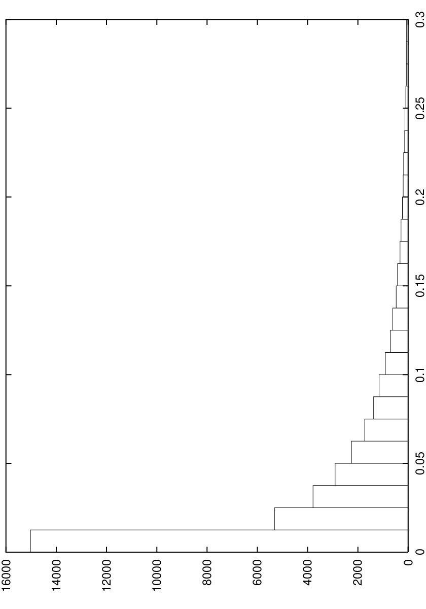
Figure 10: Distribution of the angle between the forced parton and the corresponding matrix-elements parton.

All other branchings are treated as before except that the masses of the partons not included in the history are forced to have masses below a given threshold. The matrix elements generate no emission below the mass cut at 9 GeV. The hybrid mass threshold must therefore be at least 9 GeV in order to account for the emission missing from the matrix-element part. Since no 5-parton emission is generated by the second order matrix elements, one could allow a threshold higher than 9 GeV in order to account for this potential emission. However, if any such mass is larger than one of the forced masses, the result would be a different history than the chosen one. Thus one possible mass threshold is to choose it as the smallest of the two forced masses. Another choice is a fixed mass threshold at 13 GeV, a value that gives the same average multiplicity as the original parton shower. This may be viewed as a pragmatical compromise between the two extremes above.

To show the exact execution the forced parton-shower algorithm is traced on the diagram shown in figure 8.

a

The initial partons 1 and 2 are stored in the event array. Their four-momenta are given in the center of momentum system and their spatial momentum is rotated so it coincides with the directions of the initial partons given by the matrix element and the chosen history. The directions are in this case given by $\vec{p}_{3}+\vec{p}_{5}+\vec{p}_{6}$ and $\vec{p}_{2}$ . The partons are on the mass-shell.

b

The mass of parton 1 and the $z$ value of $1\rightarrow 34$ are forced. The mass of parton 2 is chosen by solving equation (16), with the extra condition that it is below the previously mentioned threshold. The type of branching for parton 2 is also decided. Because the parton is a antiquark the only available branching is $\mathrm{\overline{q}}\rightarrow\mathrm{\overline{q}}$ g. If the branching parton is a gluon then one has to choose between branch g $\rightarrow$ gg or branch g $\rightarrow$ q $\mathrm{\overline{q}}$ . Once the branch type is chosen the z value is chosen according to one of the probabilities in (12).

c

The mass and z value of parton 3 is chosen in the same way as for parton 2 while the mass and z value of parton 4 is forced. Then the $\varphi$ angle of parton 3 and 4 is forced around the axis of parton 1.

d

Later on, after the masses of 5 and 6 have been selected, the $\varphi$ angle of parton 5 and 6 is forced. Then the parton shower is allowed to evolve in its usual way until all the partons are left on their mass-shells.

4 Results

In order to evaluate the hybrid between matrix elements and parton showers complete events are generated with parton showers, matrix elements and the hybrid. All events are generated at the $Z^{0}$ -resonance 91.2 GeV. As jet-finding algorithm the JADE scheme (technically the P0 variant [11]) is used. Only four-jet events are kept for further analysis. The three different methods have been compared in the following ways:

1.

The multiplicity distributions of charged particles are shown in figure 11. The hybrid is executed with three different mass thresholds: fixed at 13 GeV (ME+PS I), fixed at 9 GeV (ME+PS II) and minimum of the two forced masses (ME+PS III). The lower limit on jet separation is set to $d_{\mathrm{join}}=0.02$ . This choice of $d_{\mathrm{join}}$ give well separated jets and reasonable high event statistics. The distribution of the parton shower (PS) and the three hybrid distributions nearly coincide. These four distributions are also in good agreement with the experimental data [12] from the DELPHI detector at the LEP collider. The only distribution that is apparently different and doesn’t agree with the experimental data is the matrix elements distribution (ME).

Figure 11: Distributions of charged particle multiplicity
2.

The subjet multiplicity is plotted in figure 12. The number of jets is plotted as a function of the lower limit on the jet separation $d_{\mathrm{join}}\leq 0.03$ for events with four jets at $d_{\mathrm{join}}=0.03$ . Thus the subjet multiplicity gives a picture of how narrow the particles are in the four original jets. The events have been generated using the fixed mass threshold at 13 GeV. The curve corresponding to the matrix elements has the strongest tendency towards 4 jets. This is due to the fact that the matrix elements only generates 4 partons; further jets can only appear by fluctuations in the fragmentation stage.

Figure 12: subjet multiplicities
3.

The angular distributions defined in equations (21-23) are plotted in figures 13 to 15. The events have been generated using the fixed mass threshold at 13 GeV and with the lower limit on jet separation set to $d_{\mathrm{join}}=0.03$ . The distributions of the matrix element (ME) and the hybrid (ME+PS) nearly coincides for all the three angular variables while the distribution of the parton shower (PS) clearly deviates. Comparison with data is complicated, since it is difficult exactly to reproduce the experimental selection criteria, but we know [10] that the matrix elements describe them well. Thus $|\mathrm{\cos}\theta^{\ast}_{\mathrm{NR}}|$ distributions given by the hybrid, the parton shower and by experimental data [10] from the OPAL detector at LEP are scaled by the distribution given by the matrix elements. The experimental data is scaled by the ME distribution given in the referred paper while the other two distributions are scaled by the ME distribution shown in figure 14. The result is shown in figure 16. The hybrid distribution clearly matches the experimental distribution better than the parton-shower distribution does.

Refer to caption — Figure 13: $\mathrm{\cos}\chi_{\mathrm{BZ}}$ distributions

5 Summary and Outlook

The results above shows that the hybrid simulation of hadronic $\mathrm{e^{+}e^{-}}$ events gives almost the same results as the matrix elements in the case of the three angular variables $\mathrm{\cos}\chi_{\mathrm{BZ}}$ , $|\mathrm{\cos}\theta^{\ast}_{\mathrm{NR}}|$ and $\mathrm{\cos}\alpha_{34}$ . The hybrid also matches the parton showers closely when it comes to the charged particle multiplicity and the subjet multiplicity. This indicates that the hybrid gives the best total description of the hadronic $\mathrm{e^{+}e^{-}}$ four-jet events at the $\mathrm{Z^{0}}$ energy resonance.

A possible continuation of the work described in this paper is to expand the hybrid to simulations of the full second order event q $\mathrm{\overline{q}}$ +q $\mathrm{\overline{q}}$ g+q $\mathrm{\overline{q}}$ gg+q $\mathrm{\overline{q}}$ q $\mathrm{\overline{q}}$ . In such events the scale ambiguity in $\alpha_{\mathrm{s}}$ affects the rate of 4-parton events while the shape of these 4-parton events are unaffected. The first order matrix elements correction to parton showers has already been investigated by Michael H. Seymour [13]. Another much more difficult task is to apply the forced parton showers method to the description of hadron collisions.

Acknowledgment

I would like to thank my supervisor T. Sjöstrand for excellent supervision.

References

[1] F. Halzen and A. D. Martin, “Quarks & Leptons, An Introductory Course in Modern Particle Physics”, Wiley (Singapore, 1984), p. 171.
[2] R. K. Ellis, D. A. Ross and A. E. Terrano, Nucl. Phys. B178 (1981) 421.
[3] OPAL Collaboration, P.Abreu et al., Z. Phys. C59 (1993) 357.
[4] G. Altarelli and G. Parisi, Nucl. Phys. B126 (1977) 298.
[5] T. Sjöstrand, Computer Phys. Comm. 82 (1994) 74.
[6] JADE Collaboration, W. Bartel et al., Z. Phys. C33 (1986) 23;
JADE Collaboration, S. Bethke et al., Phys. Lett. B213 (1988) 235.
[7] M. Bengtsson and P. Zerwas, Phys. Lett. B206 (1988) 306.
[8] O. Nachtmann and A. Reiter, Z. Phys. C16 (1982) 45;
M. Bengtsson, Z. Phys. C42 (1989) 75.
[9] DELPHI Collaboration, P. Abreu et al., Phys. Lett. B255 (1991) 466.
[10] OPAL Collaboration, R. Akers et al., Z. Phys. C65 (1995) 367.
[11] OPAL Collaboration, M. Z. Akrawy et al., Z. Phys. C49 (1991) 375.
[12] DELPHI Collaboration, P. Abreu et al., Z. Phys. C56 (1992) 63.
[13] M. Seymour, Comp. Phys. Comm. 90 (1995) 95.