In the chiral superfield formalism, the Kähler potential, for our matter content, is commonly taken to be

$$K=-\ln Y-\sum\nolimits_{I}\ln x_{I}+\sum\nolimits_{A}X_{A},$$

(2.4)

where

$$Y=s+\bar{s}-V^{\textnormal{GS}},$$

(2.5)

with $V^{\textnormal{GS}}$ defined in (2.3). It is conventional in this formalism to write the Green-Schwarz coefficient, $b_{I}$, as²² 2 Though it is conventional in the chiral superfield formalism for the Green-Schwarz coefficient $\delta_{I}$ (or $b_{I}$) to be written with the subscript $I$, most compactifications lead to $I$ independent $\delta_{I}$.

$$b_{I}=\frac{\delta^{\textnormal{GS}}_{I}}{8\pi^{2}}.$$

(2.6)

Standard compactifications lead to $\delta^{\textnormal{GS}}_{I}\leq 30$ [9]. We will refrain from using $\delta_{I}$ to keep the clutter down in equations. The field dependence of the superpotential is

$$W=W(s,t_{I},\phi_{AI},\phi_{A}).$$

(2.7)

Its form will be given in section 2.3.

The scalar potential is made up of the $F$-term and the $D$-term: $V=V_{F}+V_{D}$. $V_{F}$ is given by

$$V_{F}=e^{K}\Bigl[K^{m\bar{n}}(W_{m}+K_{m}W)(\overline{W}_{\bar{n}}+K_{\bar{n}}\overline{W})-3|W|^{2}\Bigr],$$

(2.8)

where a subscript $m$ refers to a derivative with respect to a chiral superfield, such as $t_{I}$, and a subscript $\bar{n}$ refers to a derivative with respect to an antichiral superfield, such as $\bar{t}_{I}$. $K^{m\bar{n}}$ is the inverse of the Kähler metric, $K_{m\bar{n}}$. Both the Kähler metric and its inverse are given in appendix A.1. We will consider $V_{D}$ in section 5.1. In the absence of twisted matter, $\phi_{A}$, the scalar potential was given in [11] (see also [12]). Here, we give the scalar potential when twisted matter is included, which is

	$\displaystyle V_{F}=e^{K}$	$\displaystyle\Biggl\{-3|W|^{2}+|W-YW_{s}|^{2}$		(2.9)
		$\displaystyle+\sum\nolimits_{A}\widetilde{\Pi}_{A}^{-1}\frac{Y}{Y+p_{A}}\left|W_{A}+\widetilde{\Pi}_{A}\bar{\phi}_{A}W+p_{A}\widetilde{\Pi}_{A}\bar{\phi}_{A}W_{s}\right|^{2}$
		$\displaystyle+\sum\nolimits_{I}\frac{Y}{Y+b_{I}+\sum\nolimits_{A}q_{I}^{A}X_{A}(Y+p_{A})}$
		$\displaystyle\times\biggl[\left|x_{I}W_{I}+\sum\nolimits_{A}q_{I}^{A}\phi_{A}W_{A}-W-b_{I}W_{s}\right|^{2}+x_{I}\sum\nolimits_{A}\Bigl|\bar{\phi}_{AI}W_{I}+W_{AI}\Bigr|^{2}\biggr]\Biggr\},$

where we have defined

$$\widetilde{\Pi}_{A}\equiv\prod\nolimits_{I}x_{I}^{-q_{I}^{A}}.$$

(2.10)

In the linear superfield formalism, in the form of the Binétruy-Gaillard-Wu (BGW) model [13], the Kähler potential is [10]

$$K=\ln(\ell)+g(\ell)-\sum\nolimits_{I}\ln x_{I}+\sum\nolimits_{A}X_{A},$$

(2.11)

where $\ell$ is the dilaton in the linear superfield formalism (its relation to the dilaton in the chiral superfield formalism is given in section 2.4) and $g(\ell)$ is a nonperturbative correction that can stabilize the dilaton, which will be discussed in section 4.3. As we will see, the prescription for computing the scalar potential in this formalism requires temporarily replacing the dilaton with the (anti)chiral superfields $s$, $\bar{s}$. Hence, the field dependence of the superpotential is

$$W=W(s,t_{I},\phi_{AI},\phi_{A}).$$

(2.12)

Its general form will be given in section 2.3.

The scalar potential may be derived through the following prescription.³³ 3 Additional details may be found in Appendix A of [14]. First form

$$K^{(s)}\equiv k(s,\bar{s})-\sum\nolimits_{I}\ln x_{I}+\sum\nolimits_{A}X_{A},$$

(2.13)

which is identical to (2.11) except that the $\ell$ dependence has been replaced with a dependence on the (anti)chiral superfields $s$, $\bar{s}$. Then define the effective Kähler metric,

$$\widehat{K}_{m\bar{n}}\equiv K^{(s)}_{m\bar{n}}+\ell V^{\textnormal{GS}}_{m\bar{n}},$$

(2.14)

whose inverse is $\widehat{K}^{m\bar{n}}$ and where $V^{\textnormal{GS}}$ was defined in (2.3). Both the effective Kähler metric and its inverse are given in appendix A.2. It is conventional in this formalism to write the Green-Schwarz coefficient, $b_{I}$, as independent of $I$,⁴⁴ 4 See foonote 2.

$$b_{I}=b.$$

(2.15)

Standard compactifications lead to $b\leq 30/8\pi^{2}$ [9]. Again, the scalar potential is made up of the $F$-term and the $D$-term, but now the $F$-term is given by

$$V_{F}=e^{K}\left[\widehat{K}^{m\bar{n}}(W_{m}+K^{(s)}_{m}W)(\overline{W}_{\bar{n}}+K^{(s)}_{\bar{n}}\overline{W})-3|W|^{2}\right],$$

(2.16)

along with the replacements

$$K^{(s)}_{s}\rightarrow-\ell,\qquad\widehat{K}_{s\bar{s}}\rightarrow\frac{\ell}{\partial K/\partial\ell}=\frac{\ell^{2}}{1+\ell g^{\prime}(\ell)},$$

(2.17)

where the prime denotes differentiation with respect to $\ell$. One finds

	$\displaystyle V=e^{K}$	$\displaystyle\Biggl\{-3|W|^{2}+(\ell g^{\prime}+1)|W-\ell^{-1}W_{s}|^{2}$		(2.18)
		$\displaystyle+\sum\nolimits_{A}\widetilde{\Pi}^{-1}_{A}\frac{1}{1+p_{A}\ell}|W_{A}+\widetilde{\Pi}_{A}\bar{\phi}_{A}W+p_{A}\widetilde{\Pi}_{A}\bar{\phi}_{A}W_{s}|^{2}$
		$\displaystyle+\sum\nolimits_{I}\frac{1}{1+b\ell+\sum\nolimits_{B}(1+p_{B}\ell)q_{I}^{B}X_{B}}$
		$\displaystyle\times\biggl[\Bigl|x_{I}W_{I}+\sum\nolimits_{A}q_{I}^{A}\phi_{A}W_{A}-W-bW_{s}\Bigr|^{2}+x_{I}\sum\nolimits_{A}\Bigl|\bar{\phi}_{AI}W_{I}+W_{AI}\Bigr|^{2}\biggr]\Biggr\},$

where, as before, $\widetilde{\Pi}_{A}\equiv\prod\nolimits_{I}x_{I}^{-q_{I}^{A}}$.

The superpotential is made up of both a perturbative term and a nonperturbative term,

$$W=w_{\textnormal{p}}+w_{\textnormal{np}}.$$

(2.19)

This terminology is meant to indicate that the perturbative term leads to (pertubative) loop corrections while the nonperturbative term is induced nonperturbatively.

The perturbative term is essentially an arbitrary polynomial in the matter fields. Its precise form is dictated by the requirement of (spacetime) modular invariance, to be discussed in section 4.1. If we denote both untwisted and twisted matter by $\phi_{\alpha}$, so that $\alpha=AI$, $A$, then, for either formalism, it is given by

$$w_{\textnormal{p}}=\sum\nolimits_{m}\lambda_{m}\left[\prod\nolimits_{I}\eta(t_{I})^{-2}\right]\prod\nolimits_{\alpha}\phi_{\alpha}^{n_{m}^{\alpha}}\prod\nolimits_{J}\eta(t_{J})^{2n_{m}^{\alpha}q_{J}^{\alpha}},$$

(2.20)

where the $\lambda_{m}$ are constants, the $n_{m}^{\alpha}$ are nonnegative integers and $\eta(t_{I})$ is the Dedekind eta function,

$$\eta(t_{I})=e^{-\pi t_{I}/12}\prod_{n=1}^{\infty}\left(1-e^{-2\pi nt_{I}}\right).$$

(2.21)

The nonperturbative term follows from gaugino condensation [15]. A strongly coupled hidden sector gauge group, $G_{a}$, is expected to condense, analogously to QCD. The corresponding gaugino condensates, $u_{a}=\langle\lambda_{a}^{\alpha}\lambda^{a}_{\alpha}\rangle$, pick up nonzero VEVs, spontaneously breaking supersymmetry. If heavy enough they may be integrated out, inducing a nonperturbative contribution to the superpotential. In the chiral superfield formalism this term takes the form [13, 14]

$$w_{\textnormal{np}}=-\frac{1}{4}e^{-K/2}\sum\nolimits_{a}b_{a}u_{a},\qquad u_{a}=ce^{K/2}e^{-s/b_{a}}\prod\nolimits_{I}\left[\eta(t_{I})\right]^{2(b_{I}-b_{a})/b_{a}},$$

(2.22)

where $b_{a}$ is the $\beta$-function coefficient of the condensing gauge group and $c$ is a constant. By squaring $u_{a}$ we may write it in terms of $Y$ instead of $s$,

$$|u_{a}|^{2}=|c|^{2}e^{K}e^{-Y/b_{a}}e^{-V^{\textnormal{GS}}/b_{a}}\prod\nolimits_{I}\left|\eta(t_{I})\right|^{4(b_{I}-b_{a})/b_{a}}.$$

(2.23)

In the linear superfield formalism we have instead [13, 14]

$$w_{\textnormal{np}}=-\frac{1}{4}e^{-K/2}\sum\nolimits_{a}b_{a}u_{a},\qquad|u_{a}|^{2}=|c|^{2}e^{K}e^{-(1+f)/b_{a}\ell}e^{-V^{\textnormal{GS}}/b_{a}}\prod\nolimits_{I}\left|\eta(t_{I})\right|^{4(b-b_{a})/b_{a}},$$

(2.24)

along with the replacement

$$W_{s}\rightarrow\frac{1}{4}e^{-K/2}\sum\nolimits_{a}u_{a}.$$

(2.25)

In (2.24) $f=f(\ell)$ is uniquely determined from the nonperturbative correction $g(\ell)$ though the differential equation and boundary conditions [13]

$$\ell g^{\prime}=f-\ell f^{\prime},\qquad g(\ell=0)=f(\ell=0)=0,$$

(2.26)

where a prime denotes differentiation with respect to $\ell$.

The dilaton in the two formalisms are related by [13]

$$\frac{\ell}{1+f}=\frac{1}{s+\bar{s}-V^{\textnormal{GS}}}=\frac{1}{Y},$$

(2.27)

with $f$ defined in (2.26). If we ignore the nonperturbative term in the superpotential, then for identical perturbative terms the two formalisms are equivalent. There exists a duality transformation, made up of (2.17) and (2.27), linking them, known as chiral linear duality [7, 8]. This is manifest in the classical limit, i.e. for $f=g=0$, but also holds true in the general case. When the nonperturbative terms in the superpotential are included, it is unknown whether the two formalisms are equivalent [16]. Even with such an equivalence, it may be simpler to build models in one formalism than in the other. In the following subsections many of the results will be presented in both formalisms.⁵⁵ 5 A major exception is section 4.3 where we consider only the linear superfield formalism. However, we will find, in many different cases, that inflation model building is simpler in the linear superfield formalism.

If we denote both untwisted and twisted matter by $\phi_{\alpha}$, so that $\alpha=AI$, $A$, then modular transformations⁷⁷ 7 By modular transformations we mean specifically spacetime T-duality transformations. of the Kähler moduli and matter fields are defined by [6]

$$t_{I}\rightarrow\frac{a_{I}t_{I}-ib_{I}}{ic_{I}t_{I}+d_{I}},\qquad\phi_{\alpha}\rightarrow\phi_{\alpha}\prod\nolimits_{I}(ic_{I}t_{I}+d_{I})^{-q_{I}^{\alpha}},$$

(4.1)

where

$$a_{I}d_{I}-b_{I}c_{I}=1,\qquad a_{I},b_{I},c_{I},d_{I}\in\mathbb{Z}.$$

(4.2)

Recall that the $q_{I}^{\alpha}$ are the modular weights and that for untwisted matter fields, $q_{J}^{\alpha}=q_{J}^{AI}=\delta_{J}^{I}$, while for twisted matter fields, $q_{I}^{\alpha}=q_{I}^{A}\geq 0$.⁸⁸ 8 See footnote 1. The Kähler potential and superpotential also undergo modular transformations, which are a special case of a Kähler-Weyl transformation [24, 26],

$$K\rightarrow K+\sum\nolimits_{I}\ln|ic_{I}t_{I}+d_{I}|^{2},\qquad W\rightarrow W\prod\nolimits_{I}(ic_{I}t_{I}+d_{I})^{-1}.$$

(4.3)

Thus, the superpotential transforms with modular weight equal to 1. An important function with modular weight equal to $-1/2$ is the Dedekind eta function,

$$\eta(t_{I})=e^{-\pi t_{I}/12}\prod_{n=1}^{\infty}\left(1-e^{-2\pi nt_{I}}\right),\qquad\eta(t_{I})\rightarrow\eta(t_{I})(ic_{I}t_{I}+d_{I})^{1/2},$$

(4.4)

which tells us that the superpotential transforms as $\eta(t_{I})^{-2}$ and matter fields transform as $\eta(t_{I})^{-2q_{I}^{\alpha}}$.

Heterotic string theory is known to be modular invariant to all orders in perturbation theory [27]. This means that the effective theory must be as well. This is assured at tree level since modular transformations are just special cases of Kähler-Weyl transformations and Kähler-Weyl transformations are always symmetries of a tree level supergravity Lagrangian [24, 26]. Field theory loop corrections in general break the modular symmetry, leading to a modular anomaly. This anomaly is partially⁹⁹ 9 Threshold corrections from integrating out heavy fields cancel the remainder of the anomaly [25, 6]. canceled by introducing the Green-Schawz counterterm (2.3) [9].

We saw in section 2 that the Green-Schwarz counterterm is introduced differently in the chiral and linear superfield formalisms. In the chiral superfield formalism, the dilaton, $s+\bar{s}$, is modular invariant at tree level, but not so at loop level. For this reason, the Green-Schwarz counterterm was introduced so that the combination in (2.5) is modular invariant and the Kähler potential (2.4) transforms correctly. An important advantage of the linear superfield formalism is that the dilaton, $\ell$, is modular invariant to all orders in perturbation theory. This allows the Green-Schwarz counterterm to be introduced as in (2.14). As we will see, this will lead to simplifications.

Modular invariance also dictates the form of the perturbative term in the superpotential [13, 10]. We wrote down its form in (2.20). The eta functions in front make sure the superpotential transforms with modular weight 1, while the eta functions on the end cancel the modular transformations of the $\phi_{\alpha}$’s.

Massive states in string theory have masses on the order of the string scale ($\sim\!10^{17}$ GeV). Since an effective theory is only relevant far below this scale, all massive fields must be integrated out (leading to threshold corrections). Hence, the effective theory contains only massless fields (at least, before any fields pick up nonzero VEVs) and cannot contain mass terms. From (2.9) or (2.18) we see that the superpotential and its derivatives enter the scalar potential squared. For there to be no dimension two terms in the scalar potential, i.e. no mass terms, each term in the superpotential must be dimension three or greater. Note that this applies only to matter fields, $\phi_{\alpha}$, with moduli not included in the counting.

The method we will use for building inflation models, to be described in section 6.1, does not allow the dilaton to be the inflaton.¹⁰¹⁰ 10 In general, the dilaton as the inflaton is problematic [28]. This means that the dilaton must be stabilized, otherwise it can destroy inflation [28]. By stabilized we mean that during inflation the dilaton potential must contain a stable minimum. The method we use to achieve this, known as Kähler stabilization [13, 32, 29, 30], has been worked out in the linear superfield formalism in some detail [13, 31], where it is simpler. It has also been considered in a chiral superfield formalism without modular invariance [32]. We consider only the linear superfield formalism.

We make two further requirements. First, in the true vacuum the dilaton potential must have a stable minimum with vanishing vacuum energy,¹¹¹¹ 11 A related issue concerning dilaton stabilization in the BGW model was considered in [33]. and second, the coupling constant for the gauge fields at the string scale, $g_{s}$, must take the supersymmetric GUT value, $\approx 0.7$.

In the models we will consider the dilaton dependence during inflation is contained in the overall factor

$$V^{(\ell\>\!)}_{\textnormal{inf}}=\frac{e^{g}\ell}{1+b\ell},$$

(4.5)

where $g=g(\ell)$ is the nonperturbative correction in (2.11). In the true vacuum, using gaugino condensates to break supersymmetry and making the usual assumption that all matter fields vanish, we find that the Kähler moduli are stabilized at the fixed point $t_{I}=1$ [13]. The scalar potential in the true vacuum is then (see, for example, [31])

$$V_{0}\propto\frac{1}{b_{a}^{2}\ell^{2}}(f-f^{\prime}\ell+1)(1+b_{a}\ell)^{2}-3,$$

(4.6)

where $b_{a}$ is the $\beta$-function coefficient for the hidden sector condensing gauge group which produces the gaugino condensates, with phenomenologically preferred values $0.03\apprle b_{a}\apprle 0.04$ [34], and $f=f(\ell)$ was defined in (2.26). Finally, the coupling constant for the gauge fields at the string scale, $g_{s}$, is given by [13]

$$g_{s}^{2}=\frac{2\ell}{1+f},$$

(4.7)

where the right hand side is to be evaluated at the true vacuum.

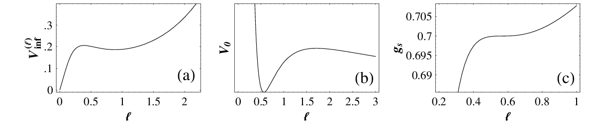
A similar (and more comprehensive) analysis of these requirements for the dilaton was made in [31], where additional phenomenological constraints were mentioned. Following [10, 31] we use only the two leading terms for the nonperturbative parameters [29],

$$f(\ell)=B\left(1+A\frac{1}{\sqrt{b\ell}}\right)e^{-1/\sqrt{b\ell}}.$$

(4.8)

In figure 1

we have plotted (4.5), (4.6) and (4.7) for the values

$$A=-0.27,\qquad B=26.8.$$

(4.9)

Figure 1(a) shows a stable minimum during inflation at $\langle\ell\rangle_{\textnormal{inf}}=0.87$, figure 1(b) shows a stable minimum with vanishing vacuum energy in the true vacuum at $\langle\ell\rangle_{0}=0.56$, and figure 1(c) shows, when evaluated at $\langle\ell\rangle_{0}=0.56$, that the coupling constant at the string scale is $0.7$.

In addition to the dilaton, the three Kähler moduli, $t_{I}$, as long as they are not the inflaton, must be stabilized. In modular invariant theories we are assured that the scalar potential will have stationary points at $t_{I}=1$, $\exp(i\pi/6)$. These two points correspond to fixed points of the modular transformation (4.1). The important question is whether the stationary points are (stable) minima.

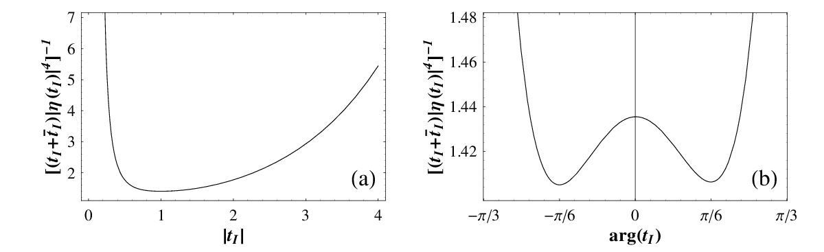
In the models we will consider the Kähler moduli dependence is often of the form

$$\left[x_{I}|\eta(t_{I})|^{4}\right]^{-1}=\left[(t_{I}+\bar{t}_{I})|\eta(t_{I})|^{4}\right]^{-1},$$

(4.10)

where we have made the usual assumption that the untwisted matter fields, $\phi_{AI}$, are negligible compared to the moduli. Setting $t_{I}=\exp(i\pi/6)+\sqrt{3}\delta$ one finds [11]

$$\left[(t_{I}+\bar{t}_{I})\left|\eta(t_{I})\right|^{4}\right]^{-1}=\frac{1}{\sqrt{3}}\left|\eta\left(e^{i\pi/6}\right)\right|^{-4}\left[1+|\delta|^{2}+O(\delta^{3})\right],$$

(4.11)

showing that $t_{I}=\exp(i\pi/6)$ corresponds to a stable minimum ($t_{I}=1$ corresponds to a saddle point). Alternatively this can be shown by plotting (4.10). Figure 2(a)

is a plot of (4.10) with $\arg(t_{I})=\pi/6$ and figure 2(b) is a plot of (4.10) with $|t_{I}|=1$. It is clear that $t_{I}=\exp(i\pi/6)$ corresponds to a stable minimum.

In many orbifold compactifications there is an anomalous $U(1)$ gauge group [35]. Canceling the anomaly requires a Green-Schwarz counterterm which leads to a Fayet-Illiopoulos contribution to the $D$-term [36]. A natural way for fields to obtain VEVs is by having them cancel such a $D$-term. The $D$-term contribution to the scalar potential is

$$V_{D}=\frac{1}{2}g^{2}\left(\sum\nolimits_{\alpha}q_{\alpha}K_{\alpha}\phi_{\alpha}+\xi_{D}\right)^{2},$$

(5.1)

where $q_{\alpha}$ is the $U(1)$ charge (and should not be confused with the modular weight) and, in the linear superfield formalism, the Fayet-Illiopoulos term is

$$\xi_{D}=\frac{2\ell\textnormal{Tr}(Q)}{192\pi^{2}},$$

(5.2)

where $\textnormal{Tr}(Q)=\sum\nolimits_{\alpha}q_{\alpha}\sim 100$ [35]. With the Kähler potential (2.11), the $D$-term (5.1) becomes

$$V_{D}=\frac{1}{2}g^{2}\left[\sum\nolimits_{\alpha}\left(\prod\nolimits_{I}x_{I}^{-q_{I}^{\alpha}}\right)q_{\alpha}|\phi_{\alpha}|^{2}+\xi_{D}\right]^{2}.$$

(5.3)

To avoid $D$-term supersymmetry breaking during inflation the matter fields must pick up the modular invariant VEVs,

$$|\langle\phi_{\alpha}\rangle|^{2}=f_{\alpha}\ell\prod\nolimits_{I}x_{I}^{q_{I}^{\alpha}},$$

(5.4)

where $f_{\alpha}$ is a constant, to cancel (5.3).

It is also possible to induce VEVs using the $F$-term of the scalar potential [10]. Consider three fields, $\chi$, $\phi_{2}$, $\phi_{3}$. Assume $\phi_{2}$, $\phi_{3}$ pick up nonzero VEVs: $\langle\phi_{2}\rangle$, $\langle\phi_{3}\rangle\neq 0$ (for example, by canceling a $D$-term). Now form the modular invariant expression

$$\Gamma=\chi\phi_{2}\phi_{3}\prod\nolimits_{I}\eta(t_{I})^{2\sum\nolimits_{\beta}q_{I}^{\beta}},\qquad\beta=\chi,2,3,$$

(5.5)

to be used in the superpotential

$$W(\Gamma)=\left[\psi\phi_{2}\phi_{3}\prod\nolimits_{I}\eta(t_{I})^{-2(1-\sum_{\gamma}q_{I}^{\gamma})}\right]\sum_{n=0}c_{n}\Gamma^{n},\quad\gamma=\psi,2,3,$$

(5.6)

where the $c_{n}$ are constants. It can be shown that, upon plugging this superpotential into the scalar potential, $\langle\psi\rangle=0$, and thus

$$V=e^{K}\prod\nolimits_{J}x_{J}^{q_{J}^{\psi}}\left|\phi_{2}\phi_{3}\prod\nolimits_{I}\eta(t_{I})^{-2(1-\sum_{\gamma}q_{I}^{\gamma})}\left[c_{0}+\sum_{n=1}c_{n}\Gamma^{n}\right]\right|^{2}.$$

(5.7)

Since $\phi_{2}$, $\phi_{3}$ are assumed to have nonzero VEVs, $\langle\chi\rangle$ is determined by

$$c_{0}+\sum_{n=1}c_{n}\Gamma^{n}=0.$$

(5.8)

The only way that (5.8) could be satisfied is if [10]

$$\Gamma=f^{3},$$

(5.9)

where $f$ is a constant, and thus

$$|\langle\chi\rangle|^{2}=|f|^{6}\left|\left<\phi_{2}\phi_{3}\prod\nolimits_{I}\eta(t_{I})^{2\sum\nolimits_{\beta}q_{I}^{\beta}}\right>\right|^{-2}.$$

(5.10)

As a first step in $F$-term inflation model building in supergravity, one must overcome the $\eta$-problem, which may be understood as follows. With the help of a Kähler-Weyl transformation and a holomorphic field redefinition a Kähler potential may be written as

$$K=\sum\nolimits_{a}|\phi_{a}|^{2}+\cdots,$$

(6.1)

where dots represent additional and, for the purpose of this subsubsection, irrelevant terms. The $F$-term contribution to the scalar potential, as we have seen above, is of the form

$$V_{F}=e^{K}(\cdots).$$

(6.2)

The slow roll parameter $\eta$, defined in (1.1), is then given by

$$\eta=1+\cdots.$$

(6.3)

Recall that slow roll inflation requires $|\eta|\ll 1$, and therefore, barring model dependent cancellations of the 1 in (6.3), slow roll inflation will not occur in a generic supergravity scalar potential. This is the $\eta$-problem.

The method we use to solve the $\eta$-problem was proposed in [11, 18], and is particularly suited for orbifold compactifications of string theory. Consider three fields, $\phi$, $\psi$, $\chi$, where $\phi$ is the inflaton. Take $\psi$ to have a small, perhaps vanishing, VEV during inflation, designated by

$$\langle\psi\rangle\sim 0.$$

(6.4)

By small we mean that $\psi$ is completely negligible in the scalar potential so that any term containing $\psi$ can be ignored (i.e. set to zero). We take this also to mean that any function which contains $\psi$ can also be ignored. In particular, the superpotential, $W(\phi,\psi,\chi)$, which is assumed to be a polynomial function of the fields in which every term contains $\psi$, during inflation satisfies

$$\langle W(\phi,\psi,\chi)\rangle\sim 0.$$

(6.5)

$\phi$ and $\chi$ derivatives do not effect the overall $\psi$ dependence of $W$ and so are small as well, $\langle W_{\phi}\rangle$, $\langle W_{\chi}\rangle\sim 0$. However, a $\psi$ derivative of $W$ removes a factor of $\psi$, and is therefore not small,

$$\left<W_{\psi}\right>\not\sim 0.$$

(6.6)

As shown by Stewart [18], for a Kähler potential of the form¹²¹² 12 Stewart actually gives the general form that the Kähler potential may take, which includes (2.1) [18]. (2.1), a $W_{\psi}$ which leads to inflation in global supersymmetry will also lead to inflation in supergravity where the inflaton can be a Kähler moduli or an untwisted matter field. Thus, inflation model building in supergravity has been rendered equivalent to inflation model building in global supersymmetry, where there is no $\eta$-problem.

As an example of what these assumptions can do, we review the superpotential presented in [10],

$$W=\lambda\psi_{1}\eta_{2}^{-2}\eta_{3}^{-2},$$

(6.7)

which is of the form (2.20) and where $\lambda$ is a constant. This superpotential does not satisfy the requirements of section 4.2. It will be generalized in section 6.3 so that it does. For now, we consider it for illustrative purposes. Plugging the superpotential (6.7) into (2.18) we obtain the scalar potential in the linear superfield formalism. It was not shown in [10] under what conditions $|\psi_{1}|=0$ will correspond to a stable minimum so that the framework of the previous subsection may be used. In appendix C.1 we show explicitly the conditions required. Assuming these conditions, so that we may set $|\psi_{1}|=0$, the scalar potential collapses down to [10]

$$V=e^{K}x_{1}\frac{|\lambda|^{2}}{|\eta_{2}\eta_{3}|^{4}}.$$

(6.8)

For the Kähler potential (2.11) this becomes [10]

$$V=\frac{\ell e^{g}}{1+b\ell}\frac{|\lambda|^{2}}{x_{2}x_{3}|\eta_{2}\eta_{3}|^{4}}.$$

(6.9)

In the chiral superfield formalism we instead find

$$V=\frac{1}{Y+b_{1}}\frac{|\lambda|^{2}}{x_{2}x_{3}|\eta_{2}\eta_{3}|^{4}}.$$

(6.10)

Notice that (6.9) is completely independent of moduli and untwisted matter from the first moduli sector ($t_{1}$ and $\phi_{1A}$). Any combination of these fields corresponds to perfect flat directions of the potential. The framework of section 6.1 has allowed us to preserve flat directions, canceling their generic lifting by supergravity, thus solving the $\eta$-problem.

In (6.10) there is an explicit dependence on these fields through the Green-Schwarz counterterm (2.3) contained in $Y$, which appears to lift the flat directions and contradict our statement in section 2.4 that the two formalisms are equivalent. In fact the flat directions do exist in (6.10); it is just more difficult to determine what they are. To do so requires diagonalizing the Kähler metric, equivalent to canonically normalizing the fields, just as we did in section 3, but now with the Green-Schwarz coefficients included—not an easy thing to do in the chiral superfield formalism.

Finally, we note two things. First, the dilaton dependence of (6.9) is precisely what we showed in section 4.3 could stabilize the dilaton during inflation and in the true vacuum, and second, the Kähler moduli dependence of (6.9) is precisely what we showed in section 4.4 would stabilize Kähler moduli.

The superpotential in section 6.2 may be generalized so that it satisfies the requirements of section 4.2 [10]. To do so, consider the superpotential

$$W_{0}=w+w^{\prime},$$

(6.11)

where

$$w=\lambda\psi_{1}\chi_{2}\phi_{2}\phi_{3}\eta_{2}^{2}.$$

(6.12)

Assume $\phi_{2}$, $\phi_{3}$ are charged under an anomalous $U(1)$ gauge group and pick up VEVs to cancel the $D$-term, as explained in section 5.1. If (6.12) were the entire superpotential (so that we did not have the contribution $w^{\prime}$ in (6.11)), we would find (under certain assumptions; see appendix C.1) that $\langle\psi_{1}\rangle=0$, which would give

$$V=e^{K}x_{1}|\langle\chi_{2}\phi_{2}\phi_{3}\rangle|^{2}|\eta_{2}|^{4}.$$

(6.13)

It would appear then that $\langle\chi_{2}\rangle=0$, but we are going to use $w^{\prime}$ in (6.11) to induce a ($F$-term) VEV for $\chi_{2}$. Following (5.6) we take

$$w^{\prime}=\psi^{\prime}_{1}\phi^{\prime}_{2}\phi^{\prime}_{3}\sum_{n=0}c_{n}\left(\chi_{2}\phi^{\prime}_{2}\phi^{\prime}_{3}\eta_{2}^{4}\eta_{3}^{2}\right)^{n}$$

(6.14)

where the primed fields in (6.14) and the unprimed fields in (6.12) are distinct, the $c_{n}$ are constants and $\phi^{\prime}_{2}$, $\phi^{\prime}_{3}$ are assumed to pick up $D$-term VEVs. Plugging the complete superpotential (6.11) (made up of (6.12) and (6.14)) into the scalar potential, we find that $\langle\psi_{1}\rangle=\langle\psi^{\prime}_{1}\rangle=0$ (see appendix C.2 for details), which gives

$$V=e^{K}x_{1}\left[\Bigl|\lambda\chi_{2}\phi_{2}\phi_{3}\eta_{2}^{2}\Bigr|^{2}+\biggl|\phi^{\prime}_{2}\phi^{\prime}_{3}\Bigr[c_{0}+\sum_{n=1}c_{n}\left(\chi_{2}\phi^{\prime}_{2}\phi^{\prime}_{3}\eta_{2}^{4}\eta_{3}^{2}\right)^{n}\Bigr]\biggr|^{2}\right].$$

(6.15)

Although $\langle\psi_{1}\rangle$ cannot be determined until the $c_{n}$ are specified, we might imagine that $V$ is minimized when the second term in (6.15) vanishes [10]. This is plausible since the term lowest order in the fields is the $c_{0}$ term and we might expect that $\langle\psi_{1}\rangle$ is determined by its cancellation. This was the case considered in section (5.2) and we assume it to be true here [10]. From (5.10) we then have [10]

$$|\langle\chi_{2}\rangle|^{2}=|f|^{6}|\langle\phi^{\prime}_{2}\phi^{\prime}_{3}\eta_{2}^{4}\eta_{3}^{2}\rangle|^{-2}.$$

(6.16)

The potential is then

$$\langle V\rangle=|\lambda|^{2}|f|^{6}\frac{f_{2}f_{3}}{f^{\prime}_{2}f^{\prime}_{3}}\frac{\ell e^{g}}{1+b\ell}\frac{1}{x_{2}x_{3}|\eta_{2}\eta_{3}|^{4}},$$

(6.17)

where we have plugged in the $D$-term VEVs of $\phi_{2}$, $\phi_{3}$, $\phi^{\prime}_{2}$, $\phi^{\prime}_{3}$ using (5.4).

In the next subsection we will consider a model in which the inflaton enters at loop level. In this subsection we review the relevant one loop corrections to the scalar potential.

In the full supergravity theory there are numerous terms in the one loop correction to the scalar potential [21, 22]. Fortunately, for the models we consider, there will be only a single term that contributes to the inflaton mass [20, 21]. To write down this term we begin by reviewing Kähler covariant notation (see, for example, [21]). First, we define

$$A\equiv e^{K}W,$$

(6.18)

with corresponding covariant derivatives

$$A_{m}=D_{m}A=\partial_{m}A=\frac{\partial}{\partial\phi_{m}}A,\qquad A_{mn}=D_{m}D_{n}A=\partial_{m}A_{n}-\Gamma^{\ell}_{mn}A_{\ell},$$

(6.19)

where the connection is defined by

$$\Gamma^{\ell}_{mn}=K^{\ell\bar{p}}\partial_{m}K_{n\bar{p}}.$$

(6.20)

With this notation we can now compactly write down the relevant loop correction. It is contained in the expression [20, 21]

$$\Delta V=2\langle V\rangle\varepsilon e^{K}A_{ij}\bar{A}^{ij},\qquad\varepsilon=\frac{\ln\Lambda}{32\pi^{2}},$$

(6.21)

where $\Lambda$ is the momentum cutoff, $\langle V\rangle$ is the tree level $F$-term contribution to the scalar potential and

$$\bar{A}=e^{K}\overline{W},\qquad\bar{A}^{mn}=K^{m\bar{\ell}}K^{n\bar{p}}\bar{A}_{\bar{\ell}\bar{p}}.$$

(6.22)

Consider now a superpotential of the form

$$W=\lambda\phi_{1}\phi_{2}\phi_{3}+\phi^{\prime}_{1}(\cdots)+\phi^{\prime\prime}_{1}(\cdots),$$

(6.23)

where $\phi_{1}$ is the inflaton, $\phi_{2}$, $\phi_{3}$, $\phi^{\prime}_{1}$, $\phi_{1}^{\prime\prime}$ are zero during inflation and the dots are any set of fields not contained in the first term nor from the same moduli sector as the inflaton (in this case $I=1$). If (6.23) leads to the tree level scalar potential $\langle V\rangle$ then by including the loop correction (6.21) it can be shown that

$$V=\langle V\rangle\left[1-4|\lambda|^{2}\varepsilon\frac{|\phi_{1}|^{2}}{t_{1}+\bar{t_{1}}-|\phi_{1}|^{2}}\right]=\langle V\rangle\Bigl[1-4|\lambda|^{2}\varepsilon\sinh^{2}(\phi)\Bigr],$$

(6.24)

where $\phi$ is the canonically normalized inflaton. Expanding this to quadratic order we have

$$V=\langle V\rangle\bigl(1-4|\lambda|^{2}\varepsilon\phi^{2}\bigr),$$

(6.25)

which is an example of a so called small field model of inflation [2, 23].

In the previous subsection we saw that to construct a model in which the inflaton dependence shows up at loop level there must be a nonzero tree level vacuum energy. Obviously the inflaton must also be missing from the tree level potential. Both of these requirements are satisfied by the potential in section 6.3. In this subsection we combine the works of [10, 20] and consider the loop corrections to that potential.

The superpotential we use is

$$W=\lambda^{\prime}\phi_{1}\phi^{\prime\prime}_{2}\phi^{\prime\prime}_{3}+W_{0},$$

(6.26)

where $W_{0}$ was given in (6.11), $\phi_{1}$ is the inflaton and both $\phi^{\prime\prime}_{2}$ and $\phi^{\prime\prime}_{3}$ have vanishing VEVs. This is of the form (6.23) and it can be shown that with the fields at their VEVs the tree level potential comes out as if the superpotential were just $W_{0}$, which was given in (6.17) (see appendix C.3),

$$\langle V\rangle=|\lambda|^{2}|f|^{6}\frac{f_{2}f_{3}}{f^{\prime}_{2}f^{\prime}_{3}}\ell e^{g}\frac{1}{x_{2}x_{3}|\eta_{2}\eta_{3}|^{4}}.$$

(6.27)

The inflaton dependence then enters at loop level, as explained in the previous subsection, yielding

$$V=\langle V\rangle\left[1-4|\lambda^{\prime}|^{2}\varepsilon\sinh^{2}(\phi)\right].$$

(6.28)

This potential stabilizes the dilaton, $t_{1}$, $t_{2}$, but does not induce a potential for $t_{1}$. For small $\phi$ during inflation,

$$V=\langle V\rangle\left(1-4|\lambda^{\prime}|^{2}\varepsilon\phi^{2}\right).$$

(6.29)

The inflaton potential in (6.29) is of the form

$$V=V_{0}\left[1-\left(\frac{\phi}{\mu}\right)^{2}\right],$$

(6.30)

with

$$V_{0}=|\lambda|^{2}|f|^{6}\frac{f_{2}f_{3}}{f^{\prime}_{2}f^{\prime}_{3}}\ell e^{g}\frac{1}{x_{2}x_{3}|\eta_{2}\eta_{3}|^{4}},\qquad\mu=\frac{1}{\sqrt{4|\lambda|^{2}\varepsilon}}.$$

(6.31)

For large $\mu$ (6.30) is an example of a small field model of inflation [2, 23]. This is precisely the situation we have since $\varepsilon$ is small, it being a loop factor. During inflation $\phi/\mu$ is usually small enough that $V\approx V_{0}$. The slow roll parameters (1.1) are then given by

$$\epsilon=\frac{2}{\mu^{2}}\left(\frac{\phi}{\mu}\right)^{2},\qquad\eta=-\frac{2}{\mu^{2}},\qquad\xi^{2}=0.$$

(6.32)

For inflation to be possible we require

$$\mu\gg\sqrt{2}$$

(6.33)

so that $|\eta|\ll 1$. Slow roll inflation ends at

$$\phi_{e}=\frac{1}{\sqrt{2}}\mu^{2},$$

(6.34)

rolling from left to right. In lieu of (6.33) inflation is ending at large field values. If we wish to restrict ourselves to small field values we must imagine that some other mechanism is acting to end inflation earlier, such as the hybrid inflation mechanism [37, 2]. We will therefore write the remaining equations in terms of an arbitrary ending field value, $\phi_{e}$.

References

- [1] A. R. Liddle and D. H. Lyth, “Cosmological inflation and large-scale structure,” Cambridge, UK: Univ. Pr. (2000).
- [2] D. H. Lyth and A. Riotto, Phys. Rept. 314, 1 (1999) [hep-ph/9807278].
- [3] D. N. Spergel et al., astro-ph/0603449; U. Seljak, A. Slosar and P. McDonald, astro-ph/0604335; A. G. Sanchez et al., Mon. Not. Roy. Astron. Soc. 366, 189 (2006) [astro-ph/0507583]; W. H. Kinney, E. W. Kolb, A. Melchiorri and A. Riotto, Phys. Rev. D 74, 023502 (2006) [astro-ph/0605338].
- [4] S. Dodelson and L. Hui, Phys. Rev. Lett. 91, 131301 (2003) [astro-ph/0305113]; A. R. Liddle and S. M. Leach, Phys. Rev. D 68, 103503 (2003) [astro-ph/0305263].
- [5] L. J. Dixon, J. A. Harvey, C. Vafa and E. Witten, Nucl. Phys. B 261, 678 (1985) and Nucl. Phys. B 274, 285 (1986).
- [6] D. Bailin and A. Love, Phys. Rept. 315, 285 (1999).
- [7] W. Siegel, Phys. Lett. B 85, 333 (1979).
- [8] P. Adamietz, P. Binetruy, G. Girardi and R. Grimm, Nucl. Phys. B 401, 257 (1993); J. P. Derendinger, F. Quevedo and M. Quiros, Nucl. Phys. B 428, 282 (1994) [hep-th/9402007]; Chapter V of P. Binetruy, G. Girardi and R. Grimm, Phys. Rept. 343, 255 (2001) [hep-th/0005225].
- [9] G. Lopes Cardoso and B. A. Ovrut, Nucl. Phys. B 369, 351 (1992); J. P. Derendinger, S. Ferrara, C. Kounnas and F. Zwirner, Nucl. Phys. B 372, 145 (1992).
- [10] M. K. Gaillard, D. H. Lyth and H. Murayama, Phys. Rev. D 58, 123505 (1998) [hep-th/9806157].
- [11] E. J. Copeland, A. R. Liddle, D. H. Lyth, E. D. Stewart and D. Wands, Phys. Rev. D 49, 6410 (1994) [astro-ph/9401011].
- [12] D. Lust and C. Munoz, Phys. Lett. B 279, 272 (1992) [hep-th/9201047].
- [13] P. Binetruy, M. K. Gaillard and Y. Y. Wu, Nucl. Phys. B 481, 109 (1996) [hep-th/9605170] and Nucl. Phys. B 493, 27 (1997) [hep-th/9611149]; M. K. Gaillard and B. D. Nelson, Int. J. Mod. Phys. A 22, 1451 (2007) [arXiv:hep-th/0703227].
- [14] P. Binetruy, M. K. Gaillard and B. D. Nelson, Nucl. Phys. B 604, 32 (2001) [hep-ph/0011081].
- [15] S. Ferrara, L. Girardello and H. P. Nilles, Phys. Lett. B 125, 457 (1983); J. P. Derendinger, L. E. Ibanez and H. P. Nilles, Phys. Lett. B 155 (1985) 65; M. Dine, R. Rohm, N. Seiberg and E. Witten, Phys. Lett. B 156 (1985) 55.
- [16] C. P. Burgess, J. P. Derendinger, F. Quevedo and M. Quiros, Phys. Lett. B 348, 428 (1995) [arXiv:hep-th/9501065].
- [17] J. Ellis, Z. Lalak, S. Pokorski and K. Turzynski, hep-th/0606133.
- [18] E. D. Stewart, Phys. Rev. D 51, 6847 (1995) [hep-ph/9405389].
- [19] P. R. Lindblom, B. A. Ovrut and P. J. Steinhardt, Phys. Lett. B 172, 309 (1986).
- [20] M. K. Gaillard, H. Murayama and K. A. Olive, Phys. Lett. B 355, 71 (1995) [arXiv:hep-ph/9504307].
- [21] M. K. Gaillard and V. Jain, Phys. Rev. D 49, 1951 (1994) [arXiv:hep-th/9308090].
- [22] M. K. Gaillard, V. Jain and K. Saririan, Phys. Rev. D 55, 883 (1997) [arXiv:hep-th/9606052] and Phys. Lett. B 387, 520 (1996) [arXiv:hep-th/9606135].
- [23] J. Martin and C. Ringeval, JCAP 0608, 009 (2006) [arXiv:astro-ph/0605367].
- [24] B. Zumino, Phys. Lett. B 87, 203 (1979).
- [25] L. J. Dixon, V. Kaplunovsky and J. Louis, Nucl. Phys. B 355, 649 (1991).
- [26] J. Wess and J. Bagger, “Supersymmetry and supergravity,” ”Princeton, USA: Univ. Pr. (1992).”
- [27] A. Giveon, N. Malkin and E. Rabinovici, Phys. Lett. B 220, 551 (1989); E. Alvarez and M. A. R. Osorio, Phys. Rev. D 40, 1150 (1989).
- [28] R. Brustein and P. J. Steinhardt, Phys. Lett. B 302, 196 (1993) [hep-th/9212049].
- [29] S. H. Shenker, in “Random surfaces and quantum gravity. Proceedings, NATO Advanced Research Workshop, Cargese, France, May 27 - June 2, 1990,” eds. O. Alvarez, E. Marinari and P. Windey, New York, USA: Plenum (1991) (NATO ASI series B, Physics, 262).
- [30] E. Silverstein, Phys. Lett. B 396, 91 (1997) [hep-th/9611195].
- [31] M. J. Cai and M. K. Gaillard, Phys. Rev. D 62, 047901 (2000) [hep-ph/9910478].
- [32] J. A. Casas, Phys. Lett. B 384, 103 (1996) [hep-th/9605180].
- [33] D. Skinner, Phys. Rev. D 67, 103506 (2003) [hep-th/0302024].
- [34] M. K. Gaillard and B. D. Nelson, Nucl. Phys. B 571, 3 (2000) [hep-ph/9909563]; A. Birkedal-Hansen and B. D. Nelson, Phys. Rev. D 64, 015008 (2001) [hep-ph/0102075] and Phys. Rev. D 67, 095006 (2003) [hep-ph/0211071].
- [35] J. Giedt, Annals Phys. 297, 67 (2002) [hep-th/0108244].
- [36] M. Dine, N. Seiberg and E. Witten, Nucl. Phys. B 289, 589 (1987); J. J. Atick, L. J. Dixon and A. Sen, Nucl. Phys. B 292, 109 (1987); M. Dine, I. Ichinose and N. Seiberg, Nucl. Phys. B 293, 253 (1987).
- [37] A. D. Linde, Phys. Lett. B 259, 38 (1991); A. D. Linde, Phys. Rev. D 49, 748 (1994) [astro-ph/9307002].