Study of the gluon propagator in the large-$N_{f}$ limit at finite temperature
and chemical potential for weak and strong couplingsPreprint: ECT*-05-07Preprint: TUW-05-11

The main technical difficulty in finding the poles of the propagator of Eq. (4), or correspondingly the zeros of the inverse propagator, is the correct analytic continuation of the self-energies from the physical sheet into the neighbouring unphysical sheet. The propagator $G(\omega+i\epsilon,q)$ neither contains poles for $\epsilon>0$ nor for $\epsilon<0$, but these two analytic regions are separated by a discontinuity along $\epsilon=0$. In order to obtain the correct pole, one has to analytically continue the function $G(\omega+i\epsilon,q)$ across this separating line from $\epsilon>0$ to $\epsilon<0$.

The self-energy components that appear in the propagator (4) can be split into a thermal piece and a vacuum piece

where the thermal pieces can be expressed as one-dimensional integrals (see Appendix A), while the vacuum part depends on a renormalization scale $\bar{\mu}$, and in the modified minimal subtraction ($\overline{{\rm MS}}$) scheme is given by

The analytic continuation of this vacuum piece is straightforward, as one just has to move the branch cut of the logarithm appropriately. One possibility is to split up the logarithm $\log(-Q^{2})\rightarrow\log(q+q_{0})+\log(q-q_{0})$. As the logarithm has a branch cut along the negative real axis, we would cross it for ${\rm Re}\,q\pm\omega<0$ when continuing $q_{0}=\omega+i\epsilon$ from $\epsilon>0$ to $\epsilon<0$. In the first logarithm we should therefore place the branch cut along the negative imaginary axis, and in the second logarithm along the positive imaginary axis. It is useful to define

where $\log(z)$ is the standard logarithmic function with a branch cut along the negative real axis. Then $\log^{\uparrow}(z)$ has the branch cut along the positive imaginary axis, $\log^{\downarrow}(z)$ has the branch cut along the negative imaginary axis, while they both agree to $\log(z)=\log^{\uparrow}(z)=\log^{\downarrow}(z)$ for ${\rm Re}(z)>0$. The analytically continued vacuum contribution can then be written by replacing

in equation (7).

The analytic continuation of the thermal self-energy functions turns out to be more involved. The expressions for $\Pi_{{\rm T,th}}$ and $\Pi_{{\rm L,th}}$, which are given in Appendix A, involve a one-dimensional integral over a real variable $k$ that has to be evaluated numerically. One might assume that it suffices to rewrite the logarithms appearing in the integrands, similar to the vacuum contribution $\Pi_{{\rm vac}}$, and leave the integration over the real variable $k$ untouched. It turns out that this prescription does not give the correct analytic continuation for the functions $\Pi_{{\rm T,th}}(q_{0},q)$ and $\Pi_{{\rm L,th}}(q_{0},q)$, as one can convince oneself by observing a discontinuity in the second derivative of the self-energies at $\epsilon=0$. Indeed, we have to be careful that the integration path for $k$ stays away from logarithmic singularities or branch cuts as we approach and penetrate the border of the physical sheet. In order to obtain the proper analytic continuation we have to deform the $k$-integration path such that crossings with singular points from the logarithms will be avoided. Another subtlety involved is that the logarithmic arguments first have to be rewritten in such a way that it is possible at all to deform the integration path satisfactorily. Details of this procedure are given in Appendix B.

For later use we note that the general form of the analytically continued inverse transverse propagator can be written as

where the renormalization scale $\bar{\mu}_{\overline{\rm MS}}$ appears explicitly in the temperature-independent vacuum piece $\Pi_{{\rm vac}}$ and implicitly in the coupling $g_{\rm eff}^{2}=g_{\rm eff}^{2}(\bar{\mu}_{\overline{\rm MS}})$, but the scalar function $f(Q/T)=\Pi_{T}(g_{\rm eff},T,Q)/(g_{\rm eff}^{2}T^{2})$ is independent of the renormalization scale $\bar{\mu}_{\overline{\rm MS}}$ as $\Pi_{T}$ is proportional to $g_{\rm eff}^{2}$ in the large-$N_{f}$ limit.

In the hard thermal loop (HTL) or hard dense loop (HDL) limit Braaten:1992gm; Frenkel:1992ts, $\Pi_{{\rm L}}$ and $\Pi_{{\rm T}}$ are given by elementary functions (listed in Appendix A.2). The HTL limit is derived by assuming soft external lines $Q\sim gT$. In this kinematical regime, the leading contribution is not only gauge independent (also beyond the large-$N_{f}$ limit), but also formally independent of the renormalization scale, as the vacuum contribution $\Pi_{{\rm vac}}$ is suppressed by $g^{2}$ compared to the leading HTL result. This leading piece is of the order of the Debye mass (HTL/HDL quantities will be marked by a hat)

which is the only scale in the HTL/HDL propagator. The HTL plasma frequency, the frequency above which there exist propagating longitudinal and transverse modes, is given by ${\hat{\omega}}_{\rm pl.}^{2}=\hat{m}_{D}^{2}/3$; the effective mass of transverse modes in the limit of large momenta (asymptotic thermal mass) by $\hat{m}_{\infty}^{2}=\hat{m}_{D}^{2}/2$.

In the large-$N_{f}$ limit, there is no such simple scaling, and the shape of the dispersion relation could in principle depend on the coupling, the temperature, and the renormalization scale. We have a restriction through the exact renormalization dependence given by Eq. (1) which means that we can basically choose a scale for plotting the dispersion relations as the result does not change if we vary renormalization scale and coupling according to the $\beta$-function.

To see how this works, let us assume that we know the position of a pole of $G(Q)$, i.e. $G^{-1}(Q)=0$. We want to show that $\bar{\mu}\partial G^{-1}(Q)/\partial\bar{\mu}=0$ is also true, provided that $g_{\rm eff}$ and $\bar{\mu}$ follow the $\beta$-function $\beta(g_{\rm eff}^{2})\equiv\bar{\mu}\,\partial g_{\rm eff}^{2}/\partial\bar{\mu}$. We find that the derivative of (11)

vanishes indeed, where we used $G_{T}^{-1}(Q)=0$ to get from the first to the second line, and the large-$N_{f}$ $\beta$-function Eq. (1) in the last line. Stated the other way round, we could have derived the $\beta$-function by demanding that $\partial G^{-1}(Q)/\partial\bar{\mu}=0$ vanishes. A similar proof holds of course for the longitudinal component as well. Also the solution $\omega(q)$ given implicitly by $G^{-1}(\omega(q),q)=0$ is independent of $\bar{\mu}_{\overline{\rm MS}}$. Since the Landau pole is also a solution to the zeros of the inverse propagator $G^{-1}(\Lambda_{{\rm Landau}})=0$, the position of the Landau pole also obeys the renormalization group equation. The same is also true for the Debye mass, which is the solution at zero frequency $\omega$ and purely imaginary $q$ for the longitudinal propagator $G_{L}^{-1}(\omega=0,q=im_{D})=0$.

Therefore, if we plot the large-$N_{f}$ dispersion relations for a specific choice of the renormalization scale, we actually plot the curve for all couplings and renormalization scales that are connected to each other by the renormalization group equation. The only problem that we might run into is the presence of the Landau pole.

Because of the presence of the Landau pole in the large-$N_{f}$ theory, the basic spectral function sum rule

valid for complex $\omega$, has to be modified. In the following, we will calculate the missing contribution. Let us first look at the zero temperature gauge field propagator. At zero temperature and zero chemical potential, $\Pi_{T}(q_{0},q)$ and $\Pi_{L}(q_{0},q)$ vanish, and one can analytically calculate the position of the Landau pole of the propagator (4) using only the vacuum self-energy (7). Solving for $G_{T}^{-1}(q_{0},q)=0$ we obtain

We define the spectral function as the discontinuity of the boson propagator along the real $q_{0}$ axis

The integral over the spectral function

can be calculated by closing the contour by a harmless grand half circle at infinity and picking up all pole contributions. The Landau pole (15) provides additional poles in the $q_{0}$ plane

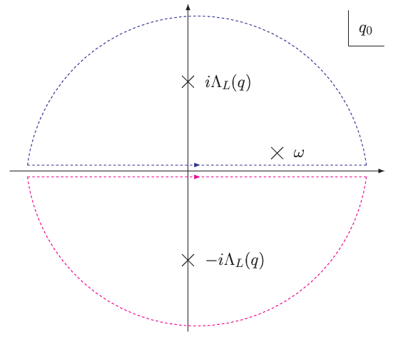
The first pole lies in the upper half of the complex plane and its residue can be calculated as:

The pole in the lower half $q_{0}=-i\Lambda_{L}(q)$ will receive an additional minus sign from the integration orientation, so that the total contribution (including the usual pole) is given by

where we have substituted back $\Lambda_{L}^{2}(q)=\Lambda_{L}^{2}-q^{2}$ with $\Lambda_{L}$ as defined in (15).

With a full one-loop self energy insertion, the position of the Landau pole $\Lambda_{L}(q)$ as the solution to $G^{-1}(q_{0}=\Lambda_{L}(q),q)=0$ for a given $q$ can in general only be calculated numerically. In the previous section we simply had $\Lambda_{L}(q)=\sqrt{\Lambda_{L}^{2}-q^{2}}$, but the dependence on $q$ is more complicated in the general case. Following the previous derivation for a general propagator, we can write the residue at the Landau pole as

Using the pole in the lower half plane and the property that the derivative of $G(q_{0},q)$ is antisymmetric along the Euclidean axis $\left.\partial G^{-1}(q_{0},q)/\partial q_{0}\right|_{q_{0}=-i\Lambda_{L}(q)}$$=-\left.\partial G^{-1}(q_{0},q)/\partial q_{0}\right|_{q_{0}=i\Lambda_{L}(q)}$ ($G(q_{0},q)$ is real and symmetric on the Euclidean axis, so its derivative is antisymmetric), the full relation is then given by

where the last part is real, despite the appearance of explicit “$i$”s. The last term corrects the usual spectral function sum rule due to the presence of the Landau pole. A rough estimate of the size of this correction can be obtained from the last term of (20): For small $Q^{2}$ it is around $5\times 10^{-7}T^{-2}$ for $g_{\rm eff}^{2}(\bar{\mu}_{\overline{\rm MS}}=\pi T)=9$ and around $2\times 10^{-3}T^{-2}$ at $g_{\rm eff}^{2}(\pi T)=36$, and increases with increasing $Q^{2}$. For soft momenta $Q\sim g_{\rm eff}T$ one could estimate roughly that this term gives a correction to the propagator of the order of $(T/\Lambda_{L})^{2}$. For hard momenta $Q\sim T$ the correction is of order $(T/g_{\rm eff}\Lambda_{L})^{2}$.

Figure 3 recalls the pressure obtained in the large-$N_{f}$ limit for finite temperature and zero quark chemical potential Moore:2002md; Ipp:2003zr; Ipp:2003jy. The full line gives the result at large $N_{f}$. The ambiguity introduced by varying the numerical cutoff below the Landau pole $Q_{{\rm max}}^{2}=a\Lambda_{L}^{2}$ between $a=1/4$ and $1/2$ is shown as a tiny (red) band for large couplings. This ambiguity is suppressed by a factor $(T/\Lambda_{L})^{4}$. Practically, this means that we can study a range of couplings $g_{\rm eff}^{2}(\bar{\mu}_{\overline{\rm MS}}=\pi T)\lesssim 36$ safely, where this number of course depends on the choice of renormalization scale $\bar{\mu}_{\overline{\rm MS}}$ [a change of this scale changes the coupling according to Eq. (2)]. Perturbation theory ceases to work much sooner and shows large scale dependences for couplings already at $g_{\rm eff}^{2}\gtrsim 4$. Using an optimized renormalization scale, namely fastest apparent convergence of the effective mass parameter $m_{{\rm E}}$ (FAC-m), the perturbative result to order $g_{\rm eff}^{5}$ follows the exact result up to $g_{\rm eff}^{2}\approx 8$. Still, there is a large range of couplings $8\lesssim g_{\rm eff}^{2}(\pi T)\lesssim 36$ to explore where strict perturbation theory fails, but the ambiguity introduced by the vicinity of the Landau pole is still negligible.

One of the remarkable and so far not easily understood features of the pressure curve is the minimum appearing at a coupling $g_{\rm eff}^{2}(\pi T)\approx 14$. Paradoxically, in this strong coupling range $g_{\rm eff}^{2}\gtrsim 14$ the pressure seems to approach again the interaction-free pressure value. Since the nontrivial content of the large-$N_{f}$ pressure can be expressed entirely in terms of the gauge boson propagator Moore:2002md; Ipp:2003zr; Ipp:2003jy, it is natural to ask whether this nonmonotonic behavior is associated with qualitative changes in the properties of the gauge boson propagator. We shall find that this is not really the case. As will be shown in a subsequent paper Birr, the nonmonotonic behavior is instead associated with nonmonotonic behavior of the asymptotic quark mass, which is a required ingredient when expressing the entropy in terms of quasiparticle spectral data Vanderheyden:1998ph; Blaizot:2000fc.

In the following we will plot spectral functions and dispersion relations covering weak and strong coupling for the gauge boson propagator in the large-$N_{f}$ limit, and compare them to the corresponding HTL results. For larger couplings, the question of renormalization scale dependence becomes important. In principle one could plot the following comparisons between exact large-$N_{f}$ and HTL results at various scales. To avoid cluttering the plots, we decided to scale large-$N_{f}$ quantities by the large-$N_{f}$ Debye mass $m_{D}$, and HTL quantities by the HTL Debye mass $\hat{m}_{D}$ and present them in the same plot. Each of the quantities is then separately renormalization scale independent, while the renormalization scale dependence of the corresponding HTL approximations can be read off separately from a plot $m_{D}/\hat{m}_{D}$. (Note that the plasma frequency would be less appropriate to set a scale of the order $\sim gT$ because of the imaginary part it obtains at larger couplings $g_{\rm eff}^{2}$ – the Debye mass on the contrary always stays purely real.) For the spectral functions we note that $g_{\rm eff}^{2}G(q_{0},q)$ and therefore $g_{\rm eff}^{2}\rho(q_{0},q)$ is a renormalization scale independent quantity.

One of the most prominent properties of the gauge boson propagator is the emergence of a screening mass in the static longitudinal sector, the Debye mass. Numerically, we obtain the Debye mass as the solution to Eq. (4) in the static limit,

While in the HTL approximation $\hat{\Pi}_{{\rm L}}(q_{0}=0,q)=\hat{m}_{D}^{2}$ is a constant given by Eq. (12), this is no longer the case for the complete expression in the large-$N_{f}$ limit. Nevertheless, the solution for $m_{D}$ indeed turns out to be a purely real number. The latter can be identified with the screening mass in a Yukawa potential for static sources. Figure 4 shows a comparison of the Debye mass in the large-$N_{f}$ limit, normalized to its corresponding HTL value (12). Other than the following plots, the axis of Fig. 4 is not labelled at a fixed renormalization scale $g_{\rm eff}^{2}(\pi T)$, but rather at a different scale for each curve as denoted next to each line. The four curves are in fact related by the renormalization group equation (2), because the position of the large-$N_{f}$ Debye mass is renormalization scale independent, like any singularity of the propagator. The HTL result on the other hand is a truncated result at order $g_{\rm eff}^{2}$. Therefore the HTL Debye mass does not run properly with the renormalization scale, leading to a renormalization-scale dependence of $m_{D}/\hat{m}_{D}$.

For small $g_{\rm eff}^{2}$ an optimal choice of renormalization scale is obtained by requiring that the $g_{\rm eff}^{4}$ contribution to the Debye mass $m_{D}$ for the full large-$N_{f}$ result vanishes. This prescription of fastest apparent convergence will be labelled as FAC-m and leads to Moore:2002md; Ipp:2003zr; Ipp:2003jy

which is very close to the choice $\bar{\mu}_{\overline{\rm MS}}=\pi T$, the lowest Matsubara frequency. Even for the largest couplings $g_{\rm eff}^{2}\approx 36$ the deviation from the HTL Debye mass is only of the order of 5% for this choice. It will therefore suffice to compare all following quantities at a fixed scale $\bar{\mu}_{\overline{\rm MS}}=\pi T$, keeping in mind that a change of the scale e.g. by a factor of 2 will introduce additional deviations as displayed in Fig. 4.

Another quantity of central importance is the plasma frequency: It indicates the lowest frequency for which there exist propagating modes in the plasma. Transverse and longitudinal modes share the same plasma frequency in an isotropic plasma. Frequencies below the plasma frequency are associated with spatial screening. The plasma frequency and the frequency of propagating modes are obtained from

While the dispersion relations obtained in the HTL approximation involve only real frequencies $\omega(q)$, the full large-$N_{f}$ result is complex. Real and imaginary parts are plotted separately in Fig. 5. Compared to the real part, the magnitude of the imaginary part remains small for all values of the coupling. For small couplings, the plasma frequency approaches the HTL value, which is given by ${\hat{\omega}}_{\rm pl.}=\hat{m}_{D}/\sqrt{3}\approx 0.57735\,\hat{m}_{D}$. As the coupling increases, the renormalization-scale independent ratio of plasma frequency to Debye mass decreases by 10% at $g_{\rm eff}^{2}(\bar{\mu}_{\overline{\rm MS}}=\pi T)=14$ and by 20% at $g_{\rm eff}^{2}=36$. The imaginary part is due to the vacuum process of quark-antiquark pair creation, which is missing in the HTL approximation. (In QCD at finite $N_{f}$, the damping rate of propagating bosonic modes is dominated by Bose-enhanced gluonic contributions proportional to a single power of $g$ rather than to $g_{\rm eff}^{2}=g^{2}N_{F}/2$ Braaten:1990it; Pisarski:1993rf; Flechsig:1995sk.)

Figures 6 and 7 show the dispersion curve for representative values of the coupling $g_{\rm eff}^{2}(\bar{\mu}=\pi T)=9$ and 36. These plots are scaled by the large-$N_{f}$ plasma frequency and thus show a renormalization scale independent result. HTL quantities are scaled by the HTL Debye mass. One notes the lower plasma frequency compared to the corresponding HTL value, albeit the effect is moderate even at large coupling. The imaginary part of the longitudinal branch vanishes quickly as the curve approaches the light-cone. In the limit of vanishing $q/m_{D}$, the real as well as the imaginary parts of transverse and longitudinal contributions coincide.⁴⁴ 4 This is due to the isotropy of the plasma. See Ref. Romatschke:2003ms for counterexamples in anisotropic plasmas within the hard-loop approximation. The unique plasma frequency at $q=0$ evolves according to Fig. 5.

Instead of assuming real wave vectors $q$ and solving numerically for complex $\omega(q)$ as we had done in Fig. 6, we could start from a given real frequency $\omega$ and calculate the corresponding complex wave vector $q(\omega)$. This corresponds to calculating the linear response to perturbations with a given real frequency. The result is shown in Figure 8 for two different couplings $g_{\rm eff}^{2}(\bar{\mu}_{\overline{\rm MS}})=9$ and 36 (which are labelled as $g_{\rm eff}=3$ and 6 respectively in the plot). Above the plasma frequency, one has weakly damped spatial oscillations, and below the plasma frequency there is predominantly exponential screening, modulated by comparatively long-range oscillations that are absent in the HTL case (though fundamentally different from the Friedel oscillations FetW:Q; Kapusta:1988fi we shall discuss further below). Following the curves down to vanishing frequency $\omega\rightarrow 0$ leads to the (real) value of the Debye mass in the longitudinal mode (right panel of Fig. 8), and in the transverse mode (left panel) to unscreened static modes (but significant dynamical screening at small but non-vanishing $\omega$). The real part of $q(\omega)$, which corresponds to spatial oscillations, vanishes for both transverse and longitudinal modes, in the static limit $\omega\rightarrow 0$. The imaginary part of the longitudinal modes for $g_{\rm eff}=3$, 6, and HTL, approaches the value 1 in the static case as the curves are normalized to this value. The HTL results of Fig. 8, which are given by dotted and dash-dotted lines, are of course independent of the coupling in units of the HTL Debye mass. In a proper comparison between large $N_{f}$ and HTL one should keep the renormalization scale dependence of $m_{D}/\hat{m}_{D}$ from Fig. 4 in mind.

Figures 9 and 10 show the spectral functions at two different values of $q/m_{D}$. The combination $T^{2}g_{\rm eff}^{2}\rho(\omega,q)$ on the ordinate is chosen in order to show a renormalization scale independent result: The quantity $g_{\rm eff}^{2}G$ is renormalization scale independent, which can be seen by combining Equations (2) and (11). In all four plots the broadening of the propagating mode peak with increasing coupling is evident. For the smaller wave vector $q/m_{D}=0.2$ in Fig. 10, one furthermore nicely observes the decrease of the plasma frequency with increasing coupling. The HTL pole corresponds to a delta function peak, indicated by the vertical line.

In the following, we extend the analysis to finite chemical potential $\mu$ and zero temperature. Figure 11 shows the corresponding Debye mass. Here the prescription of fastest apparent convergence gives

The FAC-m scale for arbitrary finite $T$ and $\mu$ can be found in Ref. Ipp:2003yz. In addition to multiples of the FAC-m scale, also the simple scale choice $\bar{\mu}_{\overline{\rm MS}}=2\mu$, varied within a factor of 4, is depicted.

For the propagating modes, Figure 12 shows the imaginary part of the dispersion relations at zero temperature for the two couplings $g_{\rm eff}^{2}=9$ and 36 at the scale $\bar{\mu}_{\overline{\rm MS}}=4\mu$. We did not plot the real part of the function separately, since they are almost indistinguishable from Figures 6 and 7 at zero chemical potential. The HDL result for the imaginary part in Fig. 12 is just zero, and the resulting imaginary part beyond HDL shows a threshold around the Fermi momentum $q\gtrsim\mu$ which can be explained as follows.

The process responsible for the imaginary part of the self-energy and thus for the propagator pole is the pair creation as shown in Figure 13. At real momenta $q$ we are looking at time-like momenta for which the Landau damping process is kinematically forbidden, even for massive quarks. The only process that could contribute to the imaginary part of the self-energy is the creation of a quark with momentum ${\bf p+{\bf q}}$ and an anti-quark with momentum ${\bf p}$. At finite chemical potential, this process is kinematically restricted as the Fermi sea is filled up to the Fermi energy $E_{F}=\mu$ and the newly produced quark must have an energy above, $\epsilon_{{\bf p+q}}\geq\mu$. The anti-quark can in principle be produced within the Fermi sea, $\epsilon_{{\bf p}}\geq 0$, but the dispersion relation of the gluon $\omega(q)$ dictates a minimal energy. From energy conservation of the process $\omega=\epsilon_{{\bf p}}+\epsilon_{{\bf p+q}}$ we obtain for the angle $\theta$ between ${\bf p}$ and ${\bf q}$

For zero mass, requiring a valid angle $-1\leq\cos\theta\leq 1$, we obtain the kinematical restriction $\omega+q\geq 2p\geq\omega-q$. For a small finite quark mass $m^{2}\leq Q^{2}=\omega^{2}-q^{2}$, the lower bound for $p$ yields

with $\gamma(Q)\equiv\sqrt{1-4m^{2}/Q^{2}}$. From the energy threshold of the quark $\epsilon_{{\bf p+q}}\geq\mu$ we immediately obtain

where $\gamma(Q)=1$ in the massless case. The momentum thresholds in Figure 12 just follow this formula $q\geq 2\mu-{\rm Re}\,\omega(q)$, scaled by the Debye mass $m_{D}$, where real part of $\omega(q)$ can be read off from Figures 6 and 7. It also explains why the momentum threshold for transverse modes is slightly lower than for the corresponding longitudinal mode, because $\omega_{T}(q)>\omega_{L}(q)$ for $q>0$.

For finite chemical potential and comparatively small temperatures, electrostatic screening at sufficiently large distances is no longer given by a simple Yukawa-type potential involving the Debye mass $m_{D}$. As is well known in nonrelativistic quantum many-body theory FetW:Q, the sharpness of the Fermi surface leads to an asymptotic behavior of the potential that is governed by so-called Friedel oscillations, implying a shell-like structure with alternating screening and overscreening. At $T=0$, the amplitude of these oscillations decays by a power law and not like an exponential. As has been shown in Ref. Kapusta:1988fi, a similar modification of Debye screening occurs in high-density QED and QCD. In the following we shall investigate this effect quantitatively in the large-$N_{f}$ theory.

The free energy of two (Abelian) static charges at a distance $r$ is given by the Fourier transform of the electrostatic gauge boson propagator Kapusta:1988fi

The deviation from Coulomb law behavior is described by the screening function

where we have used the fact that $\Pi_{L}(k_{0}=0,k)$ is an even function of $k=\sqrt{k^{2}}$. In the HTL approximation, where $\Pi_{L}(k_{0}=0,k)=\hat{m}_{D}^{2}$, one has simply $s(r)=e^{-m_{D}r}$.

However, as can be seen from the analytical results in Appendix B.4, the full gauge boson propagator at zero temperature also involves logarithmic branch cuts which touch the real axis at momenta $k=\pm 2\mu$. Following Refs. FetW:Q; Kapusta:1988fi, we separate these branch cuts infinitesimally according to $k=\pm 2\mu\pm i\epsilon$ so that the integration path of Eq. (30) is threaded through the four branch points as shown in Fig. 14. Ignoring (as implicitly done in Ref. Kapusta:1988fi) the Landau poles located at real $k=\pm\Lambda_{L}\gg\mu$ by moving them slightly into the lower half-plane, the screening function receives contributions from the Debye mass pole at $k=im_{D}$ and two integrations along the cuts starting at $k=\pm 2\mu+i\epsilon$. Because of the latter, the electrical screening at sufficiently large distances is dominated by oscillatory behavior with wavelength $\pi/\mu$. In the ultrarelativistic case the asymptotic behavior has been calculated in Ref. Kapusta:1988fi with the result

which we have transcribed to the $\overline{\rm MS}$ scheme that we are using here. Nonzero temperature moves the branch cuts away from the real axis, leading to an extra exponential suppression factor Kapusta:1988fi $e^{-2\pi Tr}$ so that they cease to govern the asymptotic behavior for $T\gtrsim m_{D}/(2\pi)$. We shall therefore concentrate on the $T=0$ case, where Friedel oscillations should be maximally important.

With regard to potential implications to high-density QED or QCD Kapusta:1988fi, it is of interest to know whether deviations from standard Debye screening occur already at moderate distances before the screening function has become negligibly small. This requires a numerical evaluation of the integral in Eq. (30) and the results for $g_{\rm eff}^{2}=9$ and $g_{\rm eff}^{2}=16$ are shown in Fig. 15. The dotted line shows the contribution from the Debye mass pole with values $m_{D}=0.94269\mu$ and $m_{D}=1.24705\mu$, respectively; the long-dashed lines labelled “Friedel” correspond to the asymptotic formula (31). The full large-$N_{f}$ result which excludes contributions from the Landau poles by moving them infinitesimally into the lower half-plane is given by the line labelled “exact”. As one can see, significant deviations from Debye screening appear only at such large distances that the screening function $s(r)$ is of the order $10^{-4}$ or below for $g_{\rm eff}^{2}=9$ and $g_{\rm eff}^{2}=16$. At these couplings, the Landau pole is at scales of the order of $10^{4}\mu$ and $3\times 10^{2}\mu$, respectively. If instead of circumventing the Landau pole we cut off the momentum integration at $a\Lambda_{L}$ with $a$ varied between $1/2$ and $1/\sqrt{2}$, this affects the screening function already considerably above the scale where Friedel oscillations occur, as shown by the dash-dotted lines in Fig. 15.⁵⁵ 5 A cutoff independent of $r$ actually would give rapid oscillations at large distances. In Fig. 15 we have instead pinned the cutoff to the last zero of the oscillatory integrand below $a\Lambda_{L}$. In real QCD, the one-loop Dyson-resummed gluon propagator also involves vacuum contributions from the gluon loop which gives asymptotic freedom and eliminates the Landau pole.⁶⁶ 6 It also introduces a branch cut lying on the imaginary axis, which is however not stable against higher-order contributions. Because of this, the results obtained by simply circumventing the Landau pole in the large-$N_{f}$ theory are probably a reasonable model of screening in high-density QCD at low temperature. Taken as such, these results suggest that Friedel oscillations occur only at distances where the screened potential is already very small. At low but nonzero temperature, the importance of Friedel oscillations is further reduced by an extra exponential suppression factor Kapusta:1988fi $e^{-2\pi Tr}$ until they disappear completely for $T\gtrsim m_{D}/(2\pi)$.

In ultrarelativistic (massless) QED, where $g_{\rm eff}^{2}\approx 0.092$, Friedel oscillations are much more suppressed than in the examples above. Ordinary Debye screening dominates out to distances $r\sim 250\mu^{-1}$, where the screening function $s\lesssim 10^{-10}$. However, Friedel oscillations in massive QED are less strongly suppressed – they then come with an extra factor of $mr$ in the screening function FetW:Q; Kapusta:1988fi. Indeed, Friedel oscillations have been seen experimentally in the nonrelativistic electron gas.

The numerical integration paths have mostly been drawn with the packages Axodraw Vermaseren:1994je and Jaxodraw Binosi:2003yf.

References

- (1) V. P. Silin, Sov. Phys. - JETP 11, 1136 (1960).
- (2) O. K. Kalashnikov and V. V. Klimov, Sov. J. Nucl. Phys. 31, 699 (1980).
- (3) V. V. Klimov, Sov. J. Nucl. Phys. 33, 934 (1981).
- (4) H. A. Weldon, Phys. Rev. D26, 1394 (1982).
- (5) H. A. Weldon, Phys. Rev. D40, 2410 (1989).
- (6) R. D. Pisarski, Nucl. Phys. A498, 423C (1989).
- (7) R. Kobes, G. Kunstatter, and A. Rebhan, Nucl. Phys. B355, 1 (1991).
- (8) E. Braaten and R. D. Pisarski, Nucl. Phys. B337, 569 (1990).
- (9) U. Kraemmer and A. Rebhan, Rept. Prog. Phys. 67, 351 (2004).
- (10) J.-P. Blaizot, E. Iancu, and A. Rebhan, in Quark-Gluon Plasma 3, edited by R. C. Hwa and X.-N. Wang (World Scientific, Singapore, 2003).
- (11) J. O. Andersen and M. Strickland, Ann. Phys. 317, 281 (2005).
- (12) G. D. Moore, JHEP 0210, 055 (2002).
- (13) A. Ipp, G. D. Moore, and A. Rebhan, JHEP 0301, 037 (2003).
- (14) A. Ipp and A. Rebhan, JHEP 0306, 032 (2003).
- (15) J.-P. Blaizot, A. Ipp, A. Rebhan, and U. Reinosa, Asymptotic thermal quark masses and the entropy of QCD in the large- limit, in preparation.
- (16) A. Peshier, K. Schertler, and M. H. Thoma, Annals Phys. 266, 162 (1998).
- (17) G. Aarts and J. M. Martinez Resco, JHEP 03, 074 (2005).
- (18) I. T. Drummond, R. R. Horgan, P. V. Landshoff, and A. Rebhan, Nucl. Phys. B524, 579 (1998).
- (19) H. J. de Vega and M. Simionato, Phys. Rev. D64, 021703 (2001).
- (20) J.-P. Blaizot and E. Iancu, Phys. Rev. D56, 7877 (1997).
- (21) E. Braaten and R. D. Pisarski, Phys. Rev. D45, 1827 (1992).
- (22) J. Frenkel and J. C. Taylor, Nucl. Phys. B374, 156 (1992).
- (23) B. Vanderheyden and G. Baym, J. Stat. Phys. 93, 843 (1998).
- (24) J.-P. Blaizot, E. Iancu, and A. Rebhan, Phys. Rev. D63, 065003 (2001).
- (25) E. Braaten and R. D. Pisarski, Phys. Rev. D42, 2156 (1990).
- (26) R. D. Pisarski, Phys. Rev. D47, 5589 (1993).
- (27) F. Flechsig, A. K. Rebhan, and H. Schulz, Phys. Rev. D52, 2994 (1995).
- (28) P. Romatschke and M. Strickland, Phys. Rev. D68, 036004 (2003).
- (29) A. L. Fetter and J. D. Walecka, Quantum Theory of Many-Particle Systems (McGraw-Hill, New York, 1971).
- (30) J. Kapusta and T. Toimela, Phys. Rev. D37, 3731 (1988).
- (31) A. Ipp, A. Rebhan, and A. Vuorinen, Phys. Rev. D69, 077901 (2004).
- (32) J. A. M. Vermaseren, Comput. Phys. Commun. 83, 45 (1994).
- (33) D. Binosi and L. Theussl, Comput. Phys. Commun. 161, 76 (2004).
- (34) K. Kajantie and J. Kapusta, Ann. Phys. 160, 477 (1985).
- (35) U. Heinz, K. Kajantie, and T. Toimela, Ann. Phys. 176, 218 (1987).
- (36) M. Kitazawa, T. Koide, T. Kunihiro, and Y. Nemoto, Pre-critical phenomena of two-flavor color superconductivity in heated quark matter: Diquark-pair fluctuations and non-Fermi liquid behavior of quarks, hep-ph/0502035.
- (37) A. Ipp, Quantum corrections to thermodynamic properties in the large limit of the quark gluon plasma, PhD thesis TU Vienna, hep-ph/0405123.