Density resummation of perturbation series in a pion gas
to leading order in chiral perturbation theory
Abstract
The mean field (MF) approximation for the pion matter, being equivalent to the Leading ChPT order, involves no dynamical loops and, if self-consistent, produces finite renormalizations only. The weight factor of the Haar measure of the pion fields, entering the path integral, generates an effective Lagrangian which is generally singular in the continuum limit. There exists one parameterization of the pion fields only, for which the weight factor is equal to unity and , respectively. This unique parameterization ensures selfconsistency of the MF approximation. We use it to calculate thermal Green functions of the pion gas in the MF approximation as a power series over the temperature. The Borel transforms of thermal averages of a function of the pion fields with respect to the scalar pion density are found to be . The perturbation series over the scalar pion density for basic characteristics of the pion matter such as the pion propagator, the pion optical potential, the scalar quark condensate , the in-medium pion decay constant , and the equation of state of pion matter appear to be asymptotic ones. These series are summed up using the contour-improved Borel resummation method. The quark scalar condensate decreases smoothly until MeV. The temperature is the maximum temperature admissible for thermalized non-linear sigma model at zero pion chemical potentials. The estimate of is above the chemical freeze-out temperature MeV at RHIC and above the phase transition to two-flavor quark matter MeV, predicted by lattice gauge theories.
pacs
11.10.Wx, 13.25.Cq, 14.40.AqI Introduction
Ultrarelativistic heavy-ion collisions allow to study phase diagram of QCD at high temperatures and small chemical potentials. Under such conditions, lattice gauge theories (LGTs) predict a crossover or a first-order phase transition into the deconfined phase, accompanied by the restoration of chiral symmetry. In two- and three-flavor LGTs, the critical temperature is estimated to be MeV and MeV with a 5% systematic error KALAPE; AALIK; Aoki06. These values are close to the chemical freeze-out temperature determined from statistical models by fitting particle yields in heavy-ion collisions BRMU01. The chemical freeze-out temperatures MeV and MeV are extracted andronic06 at top SPS energies ( GeV) and top RHIC energies ( GeV), respectively. The boundary of the phase transition might apparently be already crossed.
In ultrarelativistic heavy-ion collisions pions are the most abundant particles BRMU01; BRAV02; andronic06, so thermodynamic characteristics of a pion-dominated medium and in-medium pion properties are of current interest. At zero chemical potentials, light degrees if freedom, i.e. pions, give the dominant contribution to the pressure of hadron matter KMK, while contributions of resonances like - and -mesons with masses are suppressed as . According to the Gibbs’ criterion, the balance of pressure determines the critical temperature of the phase transition at fixed chemical potentials. The QCD phase transition can be driven therefore by pions i.e. by the lightest QCD degrees of freedom.
The energy density of a resonance gas is proportional to the small parameter which can, however, be compensated by an exponentially large amount of resonances, as has been conjectured by Hagedorn hagedorn1; hagedorn2 and discussed recently e.g. in Ref. KART. The contribution of resonances to the pressure is still suppressed in such models by a factor where GeV is a typical scale of resonance masses.
Pions are Goldstone particles and play a special role in the restoration of chiral symmetry. LGTs give an evidence that deconfinement and chiral phase transitions occur at the same critical temperature for zero chemical potentials KALA03.
Chiral perturbation theory (ChPT) exploits the invariance of strong interactions under the symmetry GL84; GL85. It has been proven to be highly successful in phenomenological descriptions of low-energy dynamics of pseudoscalar mesons MEIS; DOBA. The pion matter created in relativistic heavy-ion collisions is charge symmetric BRMU01, so the pion chemical potentials can be set equal to zero. The ChPT expansion in the vacuum runs over inverse powers of the pion decay constant MeV and, in the medium, additionally over the pion density (or temperature). Properties of the pion gas at finite temperatures, the associated chiral phase transition, and the in-medium modifications of pseudoscalar mesons within ChPT have extensively been studied GL87; GELE89; ELET93; ELET94; PITY96; BOKA96; JEON; TOUB97; dobado; KRIV; LOEWE.
The optical potential of an in-medium particle yields the self-energy operator to the first order in the density. It is determined by the forward two-body scattering amplitude on particles of the medium. ChPT is suited for calculation of the pion self-energy beyond the lowest order in density, since ChPT has all multi-pion scattering amplitudes fixed. The forward scattering amplitudes of a probing pion scattered off thermalized pions describe contributions to the in-medium pion self-energy operator. The leading ChPT amplitudes do not contain loops. This approximation is equivalent to the mean field (MF) approximation.
In this paper, we perform to the leading ChPT order the generalized Borel resummation of the asymptotic density series for the pion propagator, the pion optical potential, the scalar quark condensate , the in-medium pion decay constant , and the equation of state (EOS) of pion matter.
The outline of the paper is as follows: In the next Sect., we find for the pion field a parameterization, which provides a constant Lagrange measure for path integrals. The integration over the pion field variables is extended from to to convert path integrals to the Gaussian form. Such a procedure does apparently not affect the perturbative part of the Green functions. In Sect. III, a method for calculation of thermal averages within ChPT in the MF approximation is described. The thermal averages appear as inverse Borel transforms with respect to the non-renormalized scalar pion density. The lowest order expansion coefficients are calculated for the pion effective mass and other quantities and compared to the earlier calculations. In Sect. IV, we show that the power series with respect to the density are asymptotic and hence divergent. They can, however, be summed up with the help of the contour-improved Borel resummation technique. In Sect. V, predictions of the non-linear sigma model are compared to LTGs. The results obtained by the resummation are discussed in Conclusion.
II Pion field parameterization
The lowest order ChPT Lagrangian has the form
| (II.1) |
where is the pion mass. The kinetic term for the matrix is invariant under the chiral transformations where . The second term in Eq.(II.1) breaks chiral symmetry explicitly. In what follows, we set .
The matrix can be parameterized in various ways. The on-shell vacuum amplitudes do not depend on the choice of variables for pions CHIK; KAME. The method proposed by Gasser and Leutwyller GL84 establishes a connection between QCD Green functions and amplitudes of the effective chiral Lagrangian. Using this method, the QCD on- and off-shell amplitudes can be calculated in a way independent on the parameterization. The detailed studies of Refs. Tho95; Lee95 demonstrate that the in-medium effective meson masses are independent on the choice of meson field variables up to next-to-leading order in ChPT and to first order in density, in accordance with the equivalence theorem. The in-medium off-shell behavior and going beyond the linear-density approximation are discussed in Refs. Lee95; Par02; Kon03.
In order to provide the -matrix invariant with respect to a symmetry group, both, the action functional and the Lagrange measure entering the path integral should be invariant. The chirally invariant measure entering the path integral over the generalized coordinates coincides with the Haar measure of the group. In the exponential parameterization,
| (II.2) |
and
| (II.3) |
(see e.g. WIGN). The leading order ChPT is equivalent to the non-linear sigma model due to the isomorphism of algebras . The quantization of the non-linear sigma model MIK yields automatically the measure (II.3).
Any perturbation theory uses for dynamical fields an oscillator basis to convert path integrals into a Gaussian form. It is necessary to specify variables, , in terms of which the Lagrange measure is ”flat”:
| (II.4) |
The weight factor can always be exponentiated to generate an effective Lagrangian , in which case provides the desired parameterization. The exponential parameterization (II.2) gives, in particular, where is a lattice size. diverges in the continuum limit. The non-linear sigma model is not a renormalizable theory, so divergences cannot be absorbed into a redefinition of and . Using the MF approximation, it is usually possible to keep renormalizations finite. The exponentiation of a variable weight factor breaks, in general, selfconsistency of the MF approximation.
The divergences arising from could, however, be compensated by divergences coming from the higher orders ChPT loops. From this point of view it looks naturally to attribute to higher orders ChPT loop expansion starting from one loop. The MF approximation for the ChPT implies then that the tree level approximation neglects from the start. It is hard to expect that such an approximation is relevant at the high temperature limit where the chiral invariance is supposed to be restored.
The interaction terms in the effective Lagrangian which appear due to presence of the Haar measure have been discussed earlier in QCD WEISS; SAIL. The exponentiation of the weight factor gives consistent results due to renormalizability of QCD. The divergences appearing in the continuum limit from at a tree level are compensated by one-loop gluon self-interaction diagrams.
The consistency of the MF approximation of the non-linear sigma model survives with one parameterization only, which uses the dilatated pion fields variables such that where and
| (II.5) |
The vacuum value corresponds to , is a monotonously increasing function of . The value of has the meaning of a volume covered by a -dimensional surface of radius in a -dimensional space.
The parameterization based on the dilatation of gives , does not require the higher orders ChPT loop expansion for the consistency, and allows to work in the continuum limit with finite quantities only.
The group has a finite group volume. The magnitude of the fields is restricted by . It is generally believed that using the perturbation theory, one can extend the integrals over from to . The modification of the result is connected to large fields fluctuations of a non-perturbative nature, which do, apparently, not affect perturbation series. This conjecture is essential for the standard loop expansion in ChPT. A similar extension of the integration region is used in QCD WEISS; SAIL.
The Weinberg’s parameterization PWEIN does not restrict the magnitude of the pion fields. Such a parameterization looks especially attractive as it simplifies conversion of the path integrals into the Gaussian form. Because of the variable Lagrange measure, it can be effective starting from one loop.
The propagators (heat kernels) of free particles moving on compact group manifolds have been analyzed in Refs.DOWK; MATE; SCHU; DURU; BAAQ. It was shown that the semiclassical approximation for the propagators is exact. An explicit form of the propagator for the group is given by Schulman SCHU and Duru DURU. The problem of the variable Lagrange measure of the path integrals appears already at the quantum mechanical level. The path integral as it was recognized by Marinov and Terent’ev MATE is ill posed at the tree level. As demonstrated by Baaquie BAAQ, the divergent contributions coming from the variable Lagrange measure are cancelled by loops generated by the effective Lagrangian. A system of coupled oscillators on a compact group manifold represents unsolved problem.
The requirement of chiral invariance of the Lagrange measure being combined with the requirements that (i) the perturbation expansion is based on the oscillator basis and (ii) the MF approximation does not involve loops restricts the parameterizations of the pion fields to only one admissible parameterization.
III Thermal averages in the MF approximation
The quadratic part of the Lagrangian with respect to the fields can be extracted from Eq.(II.1) and the rest treated as a perturbation:
| (III.1) |
where is an effective pion mass to be determined self-consistently and
| (III.2) |
with
| (III.3) | |||||
| (III.4) | |||||
| (III.5) | |||||
| (III.6) |
The physical observables are expressed in terms of the thermal Green functions.
III.1 Thermal Green functions
The scalar pion density in a thermal bath with temperature is defined by
| (III.7) |
where is a renormalization constant of the pion -field and
| (III.8) |
The average (III.7) involves the normally ordered operators. The energy which enters the Bose-Einstein distribution contains the in-medium pion mass . A similar situation occurs in the Bogoliubov model of a weakly interacting non-ideal Bose gas. Also in Fermi liquid theory the momentum space distribution is determined by the in-medium dispersion law of quasi-particles (see e.g. ABRI).
In terms of thermal two-body Green function,
| (III.9) |
the momentum space distribution is determined by equation
| (III.10) |
where and
| (III.11) |
The density can be found from
| (III.12) |
where is the vacuum density of the zero-point field fluctuations
The vacuum density can be treated self-consistently beyond the lowest order ChPT only. In the MF approximation it is assumed that zero-point field fluctuations are absorbed to a redefinition of physical parameters entering the Lagrangian. In our case, the pion mass and the pion decay constant receive these contributions.
We thus neglect the vacuum fluctuations. In what follows, is set equal to zero wherever it appears. This is equivalent to using thermal part of the Green function within the loops:
| (III.13) |
Eq.(III.12) is illustrated graphically on Fig. 1. Since we neglect the zero-point field fluctuations, we may not worry on the ordering of operators, entering thermal averages such as (III.7), (III.14) and others, anymore.

III.2 In-medium pion mass and other observables
In the MF approximation, the self-energy operator can be calculated from
| (III.14) |
Equation is a consequence of the symmetry of the pion matter with respect to isospin rotations. In the momentum representation, using equation
| (III.15) |
one gets
| (III.16) |
where and
| (III.17) | |||||
| (III.18) | |||||
| (III.19) |
The self-energy operator is presented graphically on Fig. 2

Eq.(III.15) can be derived as follows: The thermal average (III.15) can be rewritten in terms of the two-body Green function
| (III.20) |
where . The two-body Green function satisfies equation
| (III.21) |
The perturbation is quadratic with respect to the derivatives, so in the MF approximation is a first order polynomial. The expansion (III.16) makes this feature explicit. Eq.(III.21) can be rewritten in the form
| (III.22) |
where is the renormalization constant introduced earlier. Using and Eqs.(III.12), (III.20), (III.22), and (A.4), we arrive at Eq.(III.15) with replaced by . The value of must be neglected, however.
The effective pion mass can be determined from equation :
| (III.23) |
while the renormalization constant is given by
| (III.24) |
The Green function in the MF approximation has the form
| (III.25) |
It is presented graphically on Fig. 3.

In what follows, we need also functions
| (III.26) | |||||
| (III.27) | |||||
which appear in calculations of density dependent renormalization constant and the pion decay constant according to Eqs. (III.29) and (III.31). Here, and are first and second derivatives with respect to .
The thermal Green function of the pion is defined by . The pion fields do not depend on derivatives of . In such a case, no additional dependence appears as compared to the propagator. Given the renormalization constant , the renormalization constant of the pion propagator can be found from
| (III.28) |
The pion propagator is shown graphically on Fig. 4.

The quark scalar condensate is proportional to the expectation value of the scalar field . The calculation of the averages and leads after factorization of isotopic indices to the calculation of averages defined in terms of functions (III.5) and (III.26):
| (III.29) | |||||
| (III.30) |

In the pion gas, the spectral density of the axial two-point function is characterized by two different pion decay constants TOUB97. In the limit , these constants coincide with . Let us find an in-medium pion decay constant, , appearing in the spectral density of the two-point function .. This definition is equivalent to equation where the right side gives the physical pion .. The axial current has the form . The calculation of the average leads after factorization of isotopic indices to the calculation of an average defined in terms of the function (III.27). In this way we obtain
| (III.31) |
III.3 Thermal averages as inverse Borel transforms
Suppose we want to find the thermal average of a function which can be expanded in a power series of . The average values of powers of the operator can be calculated as follows:
| (III.32) | |||||
The summations run for , where . In the first line, we use the multibinomial formula for . The factorization of the average in the second line is a consequence of the MF approximation according to which the averages are calculated over the free gas of quasiparticles, i.e., non-interacting effective pions in three isotopic states. In order to calculate, e.g., the average value , one has to consider permutations of the operators due to their possible pairings. Permutations inside of each pair are counted twice, whereas permutations of the pairs are counted times. This gives the factor in the third line of (III.32). To arrive at the final result one has to express in terms of Euler’s gamma functions and use their integral representations to convert tree-dimensional integral into the one-dimensional integral.
The MF approximation we used consists in the neglection of dynamical loops, i.e., loops composed from more than one dressed pion propagator. The loops composed from one dressed pion propagator give the density (III.7) after neglecting . The calculation of the average value is graphically presented on Fig.. 1 (the indices and have to be contracted with ). The calculation of the is illustrated on Fig. 5. An alternative proof of Eq.(III.32), based on the thermal Green functions method, is given in Appendix A.
The average value of can be written in the form
| (III.33) |
The thermal fluctuations are suppressed exponentially according to the value of (see also Eq.(B.7)). For small fluctuations, coincides with .
The thermal average to all orders in the pion density and to leading order in ChPT is given by the inverse Borel transform of the function .
Using the explicit form of and re-expanding results in terms of the physical density , we obtain for
| (III.34) | |||||
| (III.35) | |||||
| (III.36) | |||||
| (III.37) | |||||
| (III.38) |
For massless pions . In such a case, the power series expansions over density and temperature coincide.
The result for to order is in agreement with GL87; TOUB97; KRIV, the result for to order is in agreement with KRIV, the result for to order is in agreement with GL87; GELE89; ELET94; BOKA96; TOUB97, the result for to order is in agreement with GL87; ELET93; BOKA96; JEON.
Chiral invariance of the non-linear sigma model in the MF approximation is commented in Appendix B.
IV Summation of the density series
Most perturbation series in quantum field theory are believed to be asymptotic and hence divergent DYSON; ITZU. The integral representation (III.33) permits by changing the variable an analytical continuation into the complex half-plane , whereas at the integral diverges. The half-plane contains in general singularities the character of which depends on properties of the function . The convergence radius of the Taylor expansion is determined by the nearest singularity. One cannot exclude that the point around which we make the expansion is a singular point.
Inspecting Eqs.(III.3)-(III.6) and (III.26)-(III.27), we observe that the Borel transforms involving and are singular at where . The integral along the real half-axis of the Borel variable is therefore not feasible. Series involving such functions are asymptotic, have zero convergence radii, and are furthermore not Borel summable ITZU; BEND; JEAN.
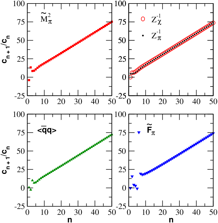
In order to clarify the character of the power series over the physical density , we calculate the higher order expansion coefficients. We write for observables (III.34)-(III.38) and plot on Fig. 6 the ratios versus up to . 11 1 The MAPLE code used to calculate the expansion coefficients is availbale upon request. The apparent asymptotic regime starts at . The ratios increase linearly with , indicating clearly that the power series are asymptotic. The slopes of these ratios are approximately equal. One can expect that the nearest singularity that appears in the series expansion over appears again in the series expansion over by virtue of . In such a case, we would expect a singularity in the Borel plane at as well. From the other side, for the Borel transform is singular at . The slope equals then , in good agreement with results presented on Fig. 6. The power series (III.34)-(III.38) with respect to the physical density have zero convergence radii and are also not Borel summable.
Generalizations of the Borel summation method have been proposed and effectively used in mathematics and atomic physics BEND; JEAN. In our case, fortunately, the residues at of the Borel transforms vanish. A contour-improved Borel resummation technique can therefore be applied which consists in a shift of the integration contour into the complex -plane. The result is stable against small variations of the contour around the positive real axis. The thermal averages, in particular, do not acquire imaginary parts and thus the expectation value, e.g., of the hermitian operator remains real. The uniqueness of the result justifies the integrations by parts of the functions , performed to derive Eqs.(III.18), (III.19), (III.29), and (III.31).

The power series (III.34)-(III.38) become summable using the contour-improved Borel resummation method.
The EOS of pion matter can be determined by averaging the energy-momentum tensor constructed from the Lagrangian (III.1). The renormalized energy density and the pressure are given by
| (IV.1) | |||||
| (IV.2) |
where . The results are plotted in Fig. 7.
There exists phenomenologically a broad interval of MeV with , covering the range of temperatures specific for heavy-ion colliders. Above MeV the renormalization constant . In the vacuum, one has as a consequence of positive definiteness of the spectral density of two-point Green functions. In the medium, the spectral density of temperature Green functions of bosons is not positive definite (see e.g. ABRI, Chap. 17-3), so does apparently not contradict unitarity. Although the product of and the pion spectral density cannot be negative, sum rule for this product is unknown. The region of self-consistency of the MF approximation within perturbation theory over the density extends up to MeV.
An interesting finite-temperature extension of the Weinberg sum rule for the product of and the spectral density of vector mesons is discussed in KAPU; ZSCH. In the MF approximation resonances do not exist, so the constraints KAPU; ZSCH apply starting from one loop ChPT.
For MeV the system has regular behavior. The scalar quark condensate decreases smoothly to zero. The effective pion mass increases with temperature in agreement with the partial restoration of chiral symmetry and approaches . The pion optical potential increases also.
The pion optical potential is calculated to all orders in density. It corresponds to the summation of the forward scattering amplitudes of a probing pion scattered on surrounding pions, with running from one to infinity.
For , . The pions disappear from the spectral density of the propagator . As elementary excitations, the pions do not disappear, however, from energy spectrum Eq.(IV.1) and contribute to the pressure Eq.(IV.2). Moreover, the pions contribute to the spectral density, e.g., of the two-point Green function .
The estimate of is significantly above the chemical freeze-out temperature MeV at RHIC.
It is worthwhile to notice that for massless pions, the scalar quark condensate vanishes at MeV. The behavior of observables (III.34)-(III.38) does not change qualitatively. EOS becomes identical with EOS of the ideal pion gas, as can be seen from Eqs.(IV.1) and (IV.2).

Let us check accuracy of presentation of the results by truncated series. In Fig. 8, we show the ratio calculated using the series expansion (III.37) truncated to orders for and . It is compared to the exact (numerical) summation of the perturbation series. We see that in the hadron phase , the first order approximation is very precise. Noticeable, irregular deviations appear beyond only. We expect, therefore, a 20% decrease of the scalar quark condensate at .
The first-order approximation is sufficiently precise for also: At , the first order of (III.34) gives for the effective pion mass , while the exact summation gives . The other observables display the similar features.
A prescription for approximate summation of asymptotic series, which is effective if initial sequential terms of asymptotic series decrease first before increasing, can be found in Ref. MIGD. One should attempt to truncate asymptotic series where two sequential terms are of the same order. The magnitude of the first neglected term gives the accuracy of the summation. Comparing and terms of (III.37), one may conclude that accuracy of the series truncated at is 100% for . One can expect that for , the accuracy is very good. As we observed, this is the case. The same arguments require be less than for . Such a requirement is satisfied also, however, with a lower precision.
V Comparison with lattice gauge theories
LGTs allow to calculate QCD observables from first principles. The smallness of physical quark masses and finite lattice spacing restrict the power of LGTs to temperatures above MeV. The non-linear sigma model, on the other hand, is an effective theory of QCD at temperatures small compared to the pion mass. There are no intrinsic restrictions to extrapolate results of the non-linear sigma model up to MeV. However, above pion mass the non-linear sigma model represents in the strict sense a model rather than an effective theory of QCD.
The phase transition to the quark matter appears in LGTs at MeV KALAPE; AALIK. The domain of validity of the non-linear sigma model is therefore limited to temperatures below . The interval of temperatures from MeV up to is suitable for a meaningful comparison of predictions from the non-linear sigma model and LTGs.

Fig. 9 shows the temperature dependence of the quark scalar condensate. The overall mass scale in LGTs is fixed assuming the string tension is flavor and quark mass independent. The agreement of the non-linear sigma model and LTG KALA03 is not unreasonable with regard to first two-three points with lowest temperatures. In the narrow deconfinement region the models strongly diverge, basically because the non-linear sigma model does not expose quark-gluon degrees of freedom.

The energy density as a function of temperature is shown in Fig. 10 at zero chemical potentials. The solid line and the dashed line are predictions of the non-linear sigma model. In addition, the lattice simulations from Refs. KALA03; KALAPE are shown.
At a first-order phase transition, the energy density experiences a jump while the pressure remains a smooth function. It is not quite clear from the LGT data presented on Fig. 10 whether we observe a crossover or a first-order phase transition. Usually, in the two-flavor case lattice simulations give evidence for a first-order phase transition, while pure gauge theory predicts a second-order transition and 2+1 flavor LGTs with physical quark masses predict a smooth crossover Aoki06.
If the phase transition is of first order , the energy density in LTG appears to be at several times greater than in the non-linear sigma model. Such a divergence can be attributed to resonances like - and -mesons which contribute to the energy density, but do not exist in the non-linear sigma model in MF approximation. An ideal resonance gas model which is in agreement with lattice simulations has e.g. been developed by Karsch et al. KART.
In the case of a first-order phase transition, the jump in the energy density can be as large as , in which case pions alone saturate the energy density. If the jump is smaller, Hagedorn’s conjecture on the exponential growth of the number of resonances with mass might be appropriate. The value of the jump is crucial in order to understand the role of higher resonances.
Modelling the first-order phase transition KMK within the framework of the MIT bag model WAIS allows to determine the critical temperature using the pressure balance where MeV/Fm3 is the vacuum pressure in flavor QCD MIT, and are pressures in quark and hadron phases, respectively, and determine jump in the energy density where and are energy densities of quark matter and hadron matter, respectively. For ideal gases of relativistic particles, , and so . The vacuum pressure is density and temperature dependent SHUR; KOBZ; MULL; DILA; ASTR; STRA, which brings to more uncertainties.
The energy density predicted by LTGs is obviously underestimated around MeV due to unphysical quark masses and restrictions from finite lattice size. The energy density and the pressure depend strongly on the quark masses and the pion mass. The horizontal part of EOS at high (dashed line and partially solid line) is close to the energy density of massless pions .

The pressure is plotted on Fig. 11. The lattice predictions KALAPE; KALA03 and the non-linear sigma model predictions are in agreement at the phase transition point, while at smaller temperatures the pressure in LGTs is significantly lower. The pressure of the pion gas approaches the pressure of ideal gas of massless pions at . However, it does not fully reach the ultrarelativistic limit, so the effects from the finite pion mass remain.
According to the Gibbs’ criterion (see e.g. LANDAF) the phase of matter with the highest presssure at equal temperatures and chemical potentials is preferable. At , heavy resonances are still slowly moving particles which contribute to the energy density mainly through their rest mass and contribute to the pressure as . For zero chemical potentials, the pressure in hadron phase is dominated by light pions KMK.
The non-linear sigma model predicts the critical pressure reasonably well. The critical temperature can be obtained phenomenologically from Fig. 11 applying the Gibbs’ criterion for the hadronic EOS derived using the non-linear sigma model and the quark matter EOS derived from LGTs. The intersection of the two pressure curves yields then the temperature of the phase transition. The value obtained in such a way is in the remarkable agreement with lattice estimates based on the position of the steep rise of the energy density seen on Fig. 10.
VI Conclusion
It is generally believed that ChPT represents an adequate tool for studying the pion matter at low temperatures. The Haar measure appearing in the path integral is important to keep the chiral symmetry at high temperatures unbroken within the MF approximation. In an arbitrary parameterization of the pion fields one faces a dilemma: Accounting for the effective potential arising due to the exponentiating the weigh factor of the path integral measure brings divergences which can be compensated by going beyond the MF approximation only, i.e., by including pion loops appearing in the higher order ChPT expansion. If is neglected, the MF approximation does not restore the chiral invariance with increasing the temperature. There is only one parameterization with , which makes the MF approximation selfconsistent: The renormalizations are finite and the chiral symmetry is restored at high temperatures. This parameterization was used to study the in-medium modifications of pions and collective characteristics of the thermalized pion matter in the MF approximation.
We made essentially two approximations:
(a) The results are obtained by extending the integration region over the pion fields from to .
(b) The MF approximation consists in the neglection of loops composed from more than one dressed pion propagator. Loops formed by one dressed pion propagator give the pion density (III.7), i.e., the thermal parts of loops are accounted for, whereas the vacuum contributions of the zero-point field fluctuations are systematically neglected. An accounting for the vacuum parts of the pion loops in a thermal bath is possible beyond the lowest ChPT order.
We constructed Borel transforms of most important thermal averages. The corresponding power series with respect to the density are asymptotic, have zero convergence radius, but are summable using the contour-improved Borel resummation method.. The pion gas does not exist above MeV, whereas at thermodynamic observables are smooth functions.
The deconfinement temperature and the corresponding scalar density appear to be small enough for approximate however quite accurate calculation of observables in hadron phase using truncated asymptotic series.
The region of validity of the method can be evaluated by requiring . The corresponding restriction MeV does not appear to be stringent.
The method of summation of the density series proposed in this work can be extended to higher orders of ChPT loop expansion.
Acknowledgements.
M.I.K. wishes to acknowledge kind hospitality at the University of Tübingen. This work has been supported by DFG grant No. 436 RUS 113/721/0-2 and RFBR grant No. 06-02-04004.Appendix A MF approximation for
The order of the operators entering the thermal average is not specified so far. As we shall see, it is not important. Let us rewrite with the help of the ordering operator . To make its action well defined, we set first arguments of the operators equal to small parameters , i.e., we make replacements . If the limit exists and does not depend on the way the parameters approach zero, the thermal average can be expressed in terms of the Green function:
| (A.1) |
In order to evaluate the Green function, we pass to the interaction representation,
| (A.2) |
where and is the thermal -matrix (see e.g. ABRI). Applying the Wick’s theorem to the -body Green function (A.2) and neglecting all the diagrams except for those corresponding to the non-interacting gas of the dressed pions, we obtain
| (A.3) |
where and are permutations of The summation runs over those permutations which occur according to the diagram decomposition of the -body Green function of a non-interacting gas. The pion propagators are dressed. Entering Eq.(A.3) are therefore the Green functions instead of .

Show on Fig. 12 are diagrams of the four-body Green function corresponding to the non-interacting gas of the effective pions. Such diagrams contribute to thermal averages. The diagram shown on Fig. 13 which accounts for the pion rescattering should be discarded in the MF approximation. This feature holds for -body Green functions. The MF approximation does not involve terms except for those entering Eq.(A.3).

The isotopic symmetry of the pion matter amounts to the two-body Green function which is symmetric under the permutation at Moreover,
| (A.4) |
Eqs.(A.3) and (A.4) imply that after neglection by all terms proportional to the limit in Eq.(A.1) exists indeed and, at least within the MF approximation, does not depend on the way the parameters approach zero. Loops formed by one pion propagator give the density (III.7), while loops involving more than one dressed pion propagator are neglected.
We obtain therefore
| (A.5) |
The combinatorial structure of the Wick’s decomposition is identical with that of the corresponding Gaussian integral, so one can write
| (A.6) | |||||
Replacing we arrive at Eq.(III.32).
Appendix B Chiral invariance in the MF approximation
As discussed in Sect. II, the MF approximation imposes restrictions on the pion field parameterizations. If the tree level is included into a MF calculation, one gets divergences. From other hand, the neglection by violates the chiral symmetry. Let us demonstrate it explicitly:
Equation (III.33) can be rewritten in more physical terms
| (B.7) |
The scalar product
| (B.8) |
is obviously chirally invariant. The value of determines the angular distance between two sets of the pion fields. The parameter space is thus a metric space with an infinitesimal distance
| (B.9) |
where and are polar and azimuthal angles of the vector .
Equation (B.7) has a transparent physical meaning. Quantum fluctuations of the fields induce fluctuations of a function . These fluctuations are suppressed by the exponential factor entering (B.7).
According to Eq.(II.5) depends on which has the meaning of a metric distance
| (B.10) |
between the vector and the vector which specifies the vacuum state on the -dimensional sphere, making thereby the chiral symmetry spontaneously broken. The only essential place in Eq.(B.7) where the dependence on the shows up is the exponential factor. In the limit the density increases, , and so the dependence on drops out. The exponential factor becomes a constant. It means that quantum fluctuations at all points of the -dimensional sphere contribute equally to thermal averages. This is in agreement with our expectations that the chiral symmetry restores with increasing the temperature.
A use of the exponential parameterization with the Haar measure neglected would result in
| (B.11) |
The Euclidean volume keeps explicitly a reference to the vacuum vector . It means that the high temperature limit does not restore the chiral invariance in the MF approximation if the Haar measure is neglected.
References
- (1) F. Karsch, E. Laermann and A. Peikert, Nucl. Phys. B605, 579 (2001).
- (2) A. Ali Khan et al., Phys. Rev. D63, 034502 (2001).
- (3) Y. Aoki, Z. Fodor, S. D. Katz and K. K. Szabo, arXiv:hep-lat/0609068.
- (4) P. Braun-Munzinger, D. Magestro, K. Reidlich, and J. Stachel, Phys. Lett. B518, 41 (2001).
- (5) A. Andronic, P. Braun-Munzinger, J. Stachel, Nucl. Phys.. A772, 167 (2006).
- (6) L. Bravina, A. Faessler, C. Fuchs, E. E. Zabrodin, Z.-D. Lu, Phys. Rev. C66, 014906 (2002).
- (7) L. A. Kondratyuk, B. V. Martemyanov, M. I. Krivoruchenko, Z. Phys. C52, 563 (1991).
- (8) F. Karsch, K. Redlich, A. Tawfik, Eur. Phys. J. C29, 549 (2003).
- (9) R. Hagedorn, Nuovo Cim. 35, 395 (1965).
- (10) R. Hagedorn, in Cargèse Lectures in Physics, Vol. 6, edited by E. Schatzman (Gordon and Breach, New York, 1973).
- (11) F. Karsch and E. Laermann, e-Print Archive: hep-lat/0305025..
- (12) J. Gasser and H. Leutwyler, Ann. Phys. 158, 142 (1984).
- (13) J. Gasser and H. Leutwyler, Nucl. Phys. B250, 465 (1985).
- (14) U. G. Meissner, Rep. Progr. Phys. 56, 903 (1993).
- (15) A. Dobado, A. N. Gómez, A. L. Maroto, and J. R. Peláez, Effective Lagrangians for the Standard Model, Springer-Verlag, Berlin (1997).
- (16) J. Gasser and H. Leutwyler, Phys. Lett. B184, 83 (1987).
- (17) P. Gerber and H. Leutwyler, Nucl. Phys. B321, 387 (1989).
- (18) V. L. Eletsky, Phys. Lett. B299, 111 (1993).
- (19) V. L. Eletsky and Ian I. Kogan, Phys. Rev. D49, 3083 (1994).
- (20) R. D. Pisarski and M. Tytgat, Phys. Rev. D54, R2989 (1996).
- (21) A. Bochkarev and J. Kapusta, Phys. Rev. D54, 4066 (1996).
- (22) S. Jeon, J. Kapusta, Phys. Rev. D54, R6475 (1996).
- (23) D. Toublan, Phys. Rev. D56, 5629 (1997).
- (24) A. Dobado, J. R. Peláez, Phys. Rev. D59, 034004 (1999).
- (25) B. V. Martemyanov, A. Faessler, C. Fuchs, M. I. Krivoruchenko, Phys. Rev. Lett. 93, 052301 (2004).
- (26) M. Loewe, C. Villavicencio, Phys. Rev. D71, 094001 (2005).
- (27) J. Chisholm, Nucl. Phys. 26, 469 (1961).
- (28) S. Kamefuchi, L. O’Raifeartaigh, and A. Salam, Nucl. Phys. 28, 529 (1961).
- (29) V. Thorsson and A. Wirzba, Nucl. Phys. A589, 633 (1995).
- (30) C.-H. Lee, G. E. Brown, D.-P. Min, and M. Rho, Nucl. Phys. A585, 401 (1995).
- (31) T.-S. Park, H. Jung, D.-P. Min, J. Kor. Phys. Soc. 41, 195 (2002).
- (32) S. Kondratyuk, K. Kubodera, F. Myhrer, Phys. Rev. C68, 044001 (2003).
- (33) E. Wigner, Group Theory, Academic, New York, 1959, p. 152.
- (34) M. I. Krivoruchenko, A. Faessler, A. A. Raduta, C. Fuchs, Phys. Lett. B608, 164 (2005).
- (35) N. Weiss, Phys. Rev. D24, 475 (1981).
- (36) K. Sailer, A. Schafer, W. Greiner, Phys. Lett. B350, 234 (1995).
- (37) S. Weinberg, Phys. Rev. 166, 1568 (1968).
- (38) J. S. Dowker, J. Phys. A 3, 451 (1970); Ann. Phys. (N.Y..) 62, 361 (1971).
- (39)
M. S. Marinov and M. V. Terent’ev, Yad. Fiz. 28, 1418 (1978) [Sov. J. Nucl. Phys. 28, 729 (1978)];
Fortschr. Phys. 27, 511 (1979). - (40) L. Schulman, Phys. Rev. 176, 1558 (1968).
- (41) I. H. Duru, Phys. Rev. D30, 2121 (1984).
- (42) B. E. Baaquie, Phys. Rev. D32, R1007 (1985).
- (43) A. A. Abrikosov, L. P. Gorkov, I. E. Dzyaloshinsky, Methods of Quantum Field Theory in Statistical Physics, Prentice-Hall, Inc. Englewood Cliffs, N. J. (1963).
- (44) F. J. Dyson, Phys. Rev. 85, 613 (1952).
- (45) C. Itzykson and J.-B. Zuber, Quantum Field Theory, McGraw-Hill, Inc. New York, 1980, Chap. 9-4.
- (46) C. M. Bender and S. A. Orszag, Advanced Mathematical Methods for Scientists and Engineers, McGraw-Hill, New York (1978).
- (47) U. D. Jentschura, Phys. Rev. A64, 013403 (2001).
- (48) J. I. Kapusta and E. V. Shuryak, Phys. Rev. D49, 4694 (1994).
- (49) S. Zschocke, O. P. Pavlenko, B. Kampfer, Eur. Phys. J. A15, 529 (2002).
- (50) A. B. Migdal, Qualitative Methods in Quantum Theory, W. A. Benjamin, Inc., Massachusetts (1977).
- (51) A. Chodos, R. L. Jaffe, K. Johnson, C. B. Thorn, V. F. Weisskopf, Phys. Rev. D9, 3471 (1974).
- (52) T. A. DeGrand, R. L. Jaffe, K. Johnson, J. E. Kiskis, Phys. Rev. D12, 2060 (1975).
- (53) E. V. Shuryak, Phys. Lett. 79, 135 (1978).
- (54) I. Yu. Kobzarev, B. V. Martemyanov, M. G. Shchepkin, Yad. Fiz. 29, 1620 (1979) [Sov. J. Nucl. Phys. 29, 831 (1979)].
- (55) B. Muller, J. Rafelski, Phys. Lett. B101, 111 (1981).
- (56) L. A. Kondratyuk, M. I. Krivoruchenko, M. G. Shchepkin, Pis’ma v ZHETF 43, 10 (1986) [JETP Lett. 43, 10 (1986)]; Yad. Fiz. 45, 514 (1987) [Sov. J. Nucl. Phys. 45, 323 (1987)].
- (57) L. A. Kondratyuk, M. I. Krivoruchenko, B. V. Martemyanov, Pis’ma v Astron. Zh. 16, 954 (1990) [Sov. Astron. Lett. 16, 410 (1990)].
- (58) N. Prasad, R. S. Bhalerao, Phys. Rev. D69, 103001 (2004).
- (59) L. Landau and E. Lifshitz, Statistical Mechanics, Pergamon, New York, (1958).