1Introduction

TUM-HEP-576/05

DESY 05-013

SHEP/0504

Running Neutrino Mass Parameters
in See-Saw Scenarios

Stefan Antusch¹¹ 1 E-mail: santusch@hep.phys.soton.ac.uk^(a), Jörn Kersten²² 2 E-mail: joern.kersten@desy.de^(b), Manfred Lindner³³ 3 E-mail: lindner@ph.tum.de^(c),
Michael Ratz⁴⁴ 4 E-mail: mratz@th.physik.uni-bonn.de^(d), and Michael Andreas Schmidt⁵⁵ 5 E-mail: mschmidt@ph.tum.de^(c)

^(a) Department of Physics and Astronomy, University of Southampton,
Southampton, SO17 1BJ, United Kingdom

^(b)Deutsches Elektronen-Synchrotron DESY, Notkestraße 85, 22603 Hamburg, Germany
^(c) Physik-Department T30, Technische Universität München
James-Franck-Straße, 85748 Garching, Germany

^(d) Physikalisches Institut der Universität Bonn,
Nussallee 12, 53115 Bonn, Germany.

We systematically analyze quantum corrections in see-saw scenarios, including effects from above as well as below the see-saw scales. We derive approximate renormalization group equations for neutrino masses, lepton mixings and CP phases, yielding an analytic understanding and a simple estimate of the size of the effects. Even for hierarchical masses, they often exceed the precision of future experiments. Furthermore, we provide a software package allowing for a convenient numerical renormalization group analysis, with heavy singlets being integrated out successively at their mass thresholds. We also discuss applications to model building and related topics.

1 Introduction

The observed smallness of neutrino masses finds an attractive explanation in the see-saw mechanism [1, 2, 3, 4, 5]. The light neutrino masses are, at tree-level, given by the famous see-saw relation

m_{\nu}\,=\,-(m_{\nu}^{\mathrm{Dirac}})^{T}\,M^{-1}\,m_{\nu}^{\mathrm{Dirac}}\;.

(1)

This relation emerges from integrating out heavy, singlet neutrinos with mass matrix $M$ . The Dirac neutrino mass $m_{\nu}^{\mathrm{Dirac}}$ is proportional to the neutrino Yukawa coupling $Y_{\nu}$ . Clearly, the see-saw operates at high energy scales while its implications are measured by experiments at low scales. Therefore, the neutrino masses given by Eq. (1) are subject to quantum corrections, i.e. they are modified by renormalization group (RG) running.

The running of neutrino masses and lepton mixing angles has been investigated intensively in the literature. For non-hierarchical neutrino mass spectra, RG effects can be very large and they can have interesting implications for model building. For example, lepton mixing angles can be magnified [6, 7, 8, 9, 10], bimaximal mixing at high energy can be compatible with low-energy experiments [11, 12, 13] or the small mass splittings can be generated from exactly degenerate light neutrinos [14, 15, 16, 17, 18, 19]. On the other hand, facing the high precision of future neutrino experiments, rather small RG corrections are important as well. For instance, deviations from $\theta_{13}=0$ or maximal mixing $\theta_{23}=\pi/4$ are induced by RG effects [20, 21, 22] also for a hierarchical spectrum. However, in most studies only the running of the dimension 5 operator has been considered, which is only appropriate for the energy range below the mass scale of the heavy singlets.

The importance of including the effects from energy ranges above and between these mass thresholds when analyzing RG effects in GUT models has been pointed out in [23, 24, 25, 26, 27, 11, 8, 12, 13, 21]. They are typically at least as important as the effects from below the thresholds since the relevant couplings, i.e. the entries of $Y_{\nu}$ , can be of order one, regardless of $\tan\beta$ .¹¹ 1 Large entries of $Y_{\nu}$ could be important in models of gauge-Yukawa unification (see, e.g., [28]), and may even be important for precision gauge unification in the MSSM [29]. Previous studies have investigated the RG effects above the see-saw scales mainly numerically.

In this paper we derive formulae which allow to understand the running of the neutrino parameters above the see-saw scales analytically. We further provide a software package for analyzing the RG evolution (with correct treatment of non-degenerate see-saw scales) numerically. We apply our results to investigate consequences of the running above the see-saw scales for model building and leptogenesis and compare the size of RG corrections to the precision of future experiments.

The paper is organized as follows: In Sec. 2, we review how the predictions for neutrino masses can be evolved from the GUT scale to the electroweak scale. Sec. 3 is dedicated to the analytic understanding of RG effects in see-saw scenarios with special emphasis on the range between $M_{\mathrm{GUT}}$ and the highest see-saw scale. In Sec. 4, we analyze the running between the see-saw scales in more detail. Sec. 5 contains a brief description of the accompanying Mathematica packages for numerical RG analyses (a detailed documentation is available at http://www.ph.tum.de/~rge/). In Sec. 6, we discuss applications to model building and related topics. Alternatives to the simplest see-saw scenario are briefly discussed in Sec. 7. Finally, Sec. 8 contains our conclusions.

2 Running Neutrino Masses in See-Saw Scenarios

In this section, we discuss how to obtain the RG evolution of neutrino masses, starting from initial conditions at a very high energy scale.²² 2 In the following we will refer to this high energy scale as $M_{\mathrm{GUT}}$ , although it can be any other scale where additional new physics, apart from the heavy singlet neutrinos, has to be taken into account. An important technical issue is that the heavy singlet neutrinos involved in the see-saw mechanism have to be integrated out one by one. Thus, one has to consider a series of effective theories [26, 27]. We will focus on the SM and the MSSM amended by three singlet neutrinos $N_{\mathrm{R}}^{i}$ or three singlet superfields $\bbnu_{i}$ , respectively. The discussion can be applied to other scenarios, such as multi-Higgs models, and a different number of singlets in a straightforward way.

We consider the Lagrangian of the SM extended by

\mathscr{L}^{\nu}=-\overline{N_{\mathrm{R}}}Y_{\nu}\ell_{\mathrm{L}}\widetilde{\phi}^{\dagger}-\frac{1}{2}\overline{N_{\mathrm{R}}}MN_{\mathrm{R}}^{\mathrm{C}}+\text{h.c.}\;,

(2)

where $\ell_{\mathrm{L}}:=(\ell_{\mathrm{L}}^{1},\ell_{\mathrm{L}}^{2},\ell_{\mathrm{L}}^{3})^{T}$ denotes the left-handed lepton doublets, $\phi$ is the Higgs doublet and $\widetilde{\phi}=i\tau^{2}\phi^{*}$ its charge conjugate. The superscript $\mathrm{C}$ denotes charge conjugation of fermion fields, and $N_{\mathrm{R}}^{\mathrm{C}}:=(N_{\mathrm{R}})^{\mathrm{C}}$ . In the supersymmetric case, $\phi$ is replaced by the Higgs doublet $H_{u}$ coupling to the up-type quarks.

In order to define mass and mixing parameters as functions of the renormalization scale $\mu$ above the highest see-saw scale, we consider the effective light neutrino mass matrix

m_{\nu}(\mu)\,=\,-\frac{v^{2}}{2}\,Y_{\nu}^{T}(\mu)\,M^{-1}(\mu)\,Y_{\nu}(\mu)\;,

(3)

where $Y_{\nu}$ and $M$ are $\mu$ -dependent. The relevant Higgs vev is $v=246\,\mathrm{GeV}$ in the SM and $v=246\,\mathrm{GeV}\cdot\sin\beta$ in the MSSM.³³ 3 As indicated in Eq. (3), we do not take into account the running of the Higgs vev. In principle, $v$ runs as well, so that $m_{\nu}$ actually does not yield the physical neutrino masses. However, the evolution of $v$ depends on the renormalization scheme and on the definition of the Higgs mass, see e.g. [30], so that there is no straightforward definition of a neutrino mass with a running vev. In any case, the mixing angles and phases are independent of the value of $v$ . This definition has shown appropriate for the applications discussed in this paper, such as leptogenesis. $m_{\nu}$ is the mass matrix of the three light neutrinos as obtained from block-diagonalizing the complete $6\times 6$ neutrino mass matrix, following the standard see-saw calculation. The scale-dependent mixing parameters are obtained from $m_{\nu}(\mu)$ and the running charged lepton Yukawa matrix $Y_{e}(\mu)$ . In Sec. 3 we are going to analyze the energy dependence of the parameters in the lepton sector such as neutrino masses, lepton mixing angles and CP phases above the highest see-saw scale analytically. Therefore, we will make use of the RGE for the composite quantity $m_{\nu}$ , calculated from those for $Y_{\nu}$ and $M$ [31, 32, 24, 25]. It is given by

16\pi^{2}\,\frac{\mathrm{d}m_{\nu}}{\mathrm{d}t}=(C_{e}\,Y_{e}^{\dagger}Y_{e}+C_{\nu}\,Y_{\nu}^{\dagger}Y_{\nu})^{T}\,m_{\nu}+m_{\nu}\,(C_{e}\,Y_{e}^{\dagger}Y_{e}+C_{\nu}\,Y_{\nu}^{\dagger}Y_{\nu})+\bar{\alpha}\,m_{\nu}

(4)

with $t:=\ln(\mu/\mu_{0})$ ,


$\displaystyle C_{e}$	$\displaystyle=-\frac{3}{2}\>,\;C_{\nu}=\frac{1}{2}$	in the SM,	(5a)
$\displaystyle C_{e}$	$\displaystyle=C_{\nu}=1$	in the MSSM,	(5b)

and (with $Y_{e}$ , $Y_{d}$ and $Y_{u}$ being the Yukawa matrices of charged leptons, down- and up-type quarks, respectively)⁴⁴ 4 We use GUT charge normalization for the gauge coupling $g_{1}$ .


$\displaystyle\bar{\alpha}_{\mathrm{SM}}$	$\displaystyle=$	$\displaystyle-\frac{9}{10}g_{1}^{2}-\frac{9}{2}g_{2}^{2}+2\Tr\big(Y_{\nu}^{\dagger}Y_{\nu}+Y_{e}^{\dagger}Y_{e}+3Y_{d}^{\dagger}Y_{d}+3Y_{u}^{\dagger}Y_{u}\big),$	(6a)
$\displaystyle\bar{\alpha}_{\mathrm{MSSM}}$	$\displaystyle=$	$\displaystyle-\frac{6}{5}g_{1}^{2}-6g_{2}^{2}+2\Tr\left(Y_{\nu}^{\dagger}Y_{\nu}+3Y_{u}^{\dagger}Y_{u}\right).$	(6b)

The RGE (4) governs only the evolution of the light neutrino mass matrix above the highest see-saw scale, which is given by the mass eigenvalue $M_{3}$ of the heaviest singlet $N_{\mathrm{R}}^{3}$ . For $\mu<M_{3}$ , we obtain the correct RG evolution by integrating out $N_{\mathrm{R}}^{3}$ . This leads to the appearance of an effective neutrino mass operator

\mathscr{L}_{\kappa}\,=\,\frac{1}{4}\,\accentset{(3)}{\kappa}_{fg}\;(\overline{\ell_{\mathrm{L}}^{\mathrm{C}}}{}^{f}\cdot\phi)\;(\ell_{\mathrm{L}}^{g}\cdot\phi)+\text{h.c.}\;,

(7)

where $f,g\in\{1,2,3\}$ are family indices and where the dot indicates the $\mathrm{SU}(2)_{\mathrm{L}}$ -invariant contractions. The coefficient of this operator is obtained by the (tree-level) matching condition⁵⁵ 5 We do not discuss finite threshold corrections, which arise due to the fact that the singlet neutrinos do not decouple abruptly [33]. The resulting uncertainty in the low-energy results is typically not larger than that due to two-loop effects. In the \hrefhttp://www.ph.tum.de/ rge/REAP software package described in Sec. 5, the corrections can be implemented approximately by integrating out $N_{\mathrm{R}}^{3}$ slightly below $M_{3}$ .

\accentset{(3)}{\kappa}_{gf}\,=\,2(Y_{\nu}^{T})_{g3}\,M^{-1}_{3}\,(Y_{\nu})_{3f}\;,

(8)

which is imposed at $\mu=M_{3}$ . This expression is specified in the mass basis for the singlets, i.e. in the basis where $M$ is diagonal. Let us mention that finding the matching scale properly requires some care as the mass matrix $M$ (and consequently the eigenvalue $M_{3}$ ) itself is subject to the RG evolution. As a consequence, for scales below $M_{3}$ the effective neutrino mass matrix can be described as a sum of two contributions,

m_{\nu}\,=\,-\frac{v^{2}}{4}\raise 1.5pt\hbox{$\displaystyle\bigl($}\,\accentset{(3)}{\kappa}+2\,\accentset{(3)}{Y}_{\nu}^{T}\accentset{(3)}{M}^{-1}\accentset{(3)}{Y}_{\nu}\raise 1.5pt\hbox{$\displaystyle\bigr)$}\;.

(9)

The $2\times 3$ Yukawa matrix $\accentset{(3)}{Y}_{\nu}$ is obtained by simply removing the last row of $Y_{\nu}$ in the basis where $M$ is diagonal. The $2\times 2$ mass matrix $\accentset{(3)}{M}$ is found from $M$ by removing the last row and column. By construction, $m_{\nu}$ is a continuous function of the renormalization scale. The RG evolution of the second term on the right-hand side of Eq. (9) is governed by Eq. (4) with $Y_{\nu}$ replaced by $\accentset{(3)}{Y}_{\nu}$ . The running of the first term, on the other hand, is determined by the RGE [27]

16\pi^{2}\,\frac{\mathrm{d}\,\accentset{(3)}{\kappa}}{\mathrm{d}t}=\raise 1.5pt\hbox{$\displaystyle\bigl($}C_{e}\,Y_{e}^{\dagger}Y_{e}+C_{\nu}\,\accentset{(3)}{Y}_{\nu}^{\dagger}\accentset{(3)}{Y}_{\nu}\raise 1.5pt\hbox{$\displaystyle\bigr)$}^{T}\,\accentset{(3)}{\kappa}+\accentset{(3)}{\kappa}\,\raise 1.5pt\hbox{$\displaystyle\bigl($}C_{e}\,Y_{e}^{\dagger}Y_{e}+C_{\nu}\,\accentset{(3)}{Y}_{\nu}^{\dagger}\accentset{(3)}{Y}_{\nu}\raise 1.5pt\hbox{$\displaystyle\bigr)$}+\accentset{(3)}{\bar{\alpha}}\;\accentset{(3)}{\kappa}

(10)

with $C_{e}$ and $C_{\nu}$ as in Eqs. (5) [34, 35, 36, 37], and


$\displaystyle\accentset{(3)}{\bar{\alpha}}_{\mathrm{SM}}$	$\displaystyle=$	$\displaystyle-3g_{2}^{2}+2\Tr\!\raise 1.5pt\hbox{$\displaystyle\bigl($}\accentset{(3)}{Y}^{\dagger}_{\nu}\accentset{(3)}{Y}_{\nu}+Y_{e}^{\dagger}Y_{e}+3Y_{d}^{\dagger}Y_{d}+3Y_{u}^{\dagger}Y_{u}\raise 1.5pt\hbox{$\displaystyle\bigr)$}+\lambda\;,$	(11a)
$\displaystyle\accentset{(3)}{\bar{\alpha}}_{\mathrm{MSSM}}$	$\displaystyle=$	$\displaystyle-\frac{6}{5}g_{1}^{2}-6g_{2}^{2}+2\Tr\!\raise 1.5pt\hbox{$\displaystyle\bigl($}\accentset{(3)}{Y}^{\dagger}_{\nu}\accentset{(3)}{Y}_{\nu}+3Y_{u}^{\dagger}Y_{u}\raise 1.5pt\hbox{$\displaystyle\bigr)$}\;.$	(11b)

One can now evolve the effective neutrino mass matrix down to the scale $M_{2}$ and repeat the matching procedure there. From integrating out $N_{\mathrm{R}}^{2}$ at $\mu=M_{2}$ , the Yukawa matrix gets further reduced and the effective neutrino mass operator receives an additional contribution. After a subsequent RG evolution to $\mu=M_{1}$ , the procedure is repeated for $N_{\mathrm{R}}^{1}$ . The emerging effective theories, as well as the quantities relevant to neutrino masses in each of them, are illustrated in Fig. 1.

Refer to caption — Figure 1: Validity ranges of the effective theories (EFTs) in the renormalization scale $\mu$ . At a scale close to the mass thresholds $M_{i}$ , the EFTs are related by matching conditions. Although we show this illustration for 3 heavy singlets, it is straightforward to generalize it to an arbitrary number (cf. [27]).

In summary, the running of the effective neutrino mass matrix $m_{\nu}$ above and between the see-saw scales is given by the running of two parts,

m_{\nu}\,=\,-\frac{v^{2}}{4}\raise 1.5pt\hbox{$\displaystyle\bigl($}\,\accentset{(n)}{\kappa}+2\,\accentset{(n)}{Y}_{\nu}^{T}\accentset{(n)}{M}^{-1}\accentset{(n)}{Y}_{\nu}\raise 1.5pt\hbox{$\displaystyle\bigr)$}\;.

(12)

where $n$ labels the effective theory (cf. Fig. 1). In the SM and the MSSM, the 1-loop $\beta$ -functions for $m_{\nu}$ in the various effective theories can be summarized as

\displaystyle 16\pi^{2}\,\frac{\mathrm{d}\accentset{(n)}{X}}{\mathrm{d}t}

\displaystyle=

\displaystyle\vphantom{\frac{1}{2}}\raise 1.5pt\hbox{$\displaystyle\bigl($}C_{e}Y_{e}^{\dagger}Y_{e}+C_{\nu}\accentset{(n)}{Y}^{\dagger}_{\nu}\accentset{(n)}{Y}_{\nu}\raise 1.5pt\hbox{$\displaystyle\bigr)$}^{T}\>\accentset{(n)}{X}+\accentset{(n)}{X}\,\raise 1.5pt\hbox{$\displaystyle\bigl($}C_{e}Y_{e}^{\dagger}Y_{e}+C_{\nu}\accentset{(n)}{Y}^{\dagger}_{\nu}\accentset{(n)}{Y}_{\nu}\raise 1.5pt\hbox{$\displaystyle\bigr)$}+\accentset{(n)}{\bar{\alpha}}_{X}\accentset{(n)}{X}\;,

(13)

where $\accentset{(n)}{X}$ stands for $\accentset{(n)}{\kappa}$ or for $2\,\accentset{(n)}{Y}_{\nu}^{T}\accentset{(n)}{M}^{-1}\accentset{(n)}{Y}_{\nu}$ , respectively. The coefficients $C_{i}$ and $\bar{\alpha}_{i}$ are listed in Tab. 1.

Model	$\accentset{(n)}{X}$	$\!C_{e}\!$	$\!C_{\nu}\!$	flavour-trivial term $\accentset{(n)}{\bar{\alpha}}_{X}$
SM	$\accentset{(n)}{\kappa}$	$\!-\tfrac{3}{2}\!$	$\tfrac{1}{2}$	$2\Tr\raise 1.5pt\hbox{$\displaystyle\bigl($}\accentset{(n)}{Y}^{\dagger}_{\nu}\accentset{(n)}{Y}_{\nu}+Y_{e}^{\dagger}Y_{e}+3Y_{d}^{\dagger}Y_{d}+3Y_{u}^{\dagger}Y_{u}\raise 1.5pt\hbox{$\displaystyle\bigr)$}-3g_{2}^{2}+\lambda$
SM	$2\,\accentset{(n)}{Y}_{\nu}^{T}\accentset{(n)}{M}^{-1}\accentset{(n)}{Y}_{\nu}\!\!$	$\!-\tfrac{3}{2}\!$	$\tfrac{1}{2}$	$2\Tr\raise 1.5pt\hbox{$\displaystyle\bigl($}\accentset{(n)}{Y}^{\dagger}_{\nu}\accentset{(n)}{Y}_{\nu}+Y_{e}^{\dagger}Y_{e}+3Y_{d}^{\dagger}Y_{d}+3Y_{u}^{\dagger}Y_{u}\raise 1.5pt\hbox{$\displaystyle\bigr)$}-\tfrac{9}{10}g_{1}^{2}-\tfrac{9}{2}g_{2}^{2}$
MSSM	$\accentset{(n)}{\kappa}$	$1$	$1$	$2\Tr\raise 1.5pt\hbox{$\displaystyle\bigl($}\accentset{(n)}{Y}^{\dagger}_{\nu}\accentset{(n)}{Y}_{\nu}+3Y_{u}^{\dagger}Y_{u}\raise 1.5pt\hbox{$\displaystyle\bigr)$}-\tfrac{6}{5}g_{1}^{2}-6g_{2}^{2}$
MSSM	$2\,\accentset{(n)}{Y}_{\nu}^{T}\accentset{(n)}{M}^{-1}\accentset{(n)}{Y}_{\nu}\!\!$	$1$	$1$	$2\Tr\raise 1.5pt\hbox{$\displaystyle\bigl($}\accentset{(n)}{Y}^{\dagger}_{\nu}\accentset{(n)}{Y}_{\nu}+3Y_{u}^{\dagger}Y_{u}\raise 1.5pt\hbox{$\displaystyle\bigr)$}-\tfrac{6}{5}g_{1}^{2}-6g_{2}^{2}$

Table 1: Coefficients of the

\beta

-functions of Eq. (13), which govern the running of the effective neutrino mass matrix in minimal see-saw models.

3 Analytic Understanding of the RG Evolution

The methods of [38, 31, 39, 20] can be used to derive differential equations for the running of the neutrino masses, mixing angles and CP phases in the see-saw scenario. In this section, we concentrate on the full theory above the highest see-saw scale. The corresponding differential equations for the running below the see-saw scales have been discussed in [40, 39, 20]. We abbreviate the flavour-dependent terms in the RGE (4) by

P:=C_{e}\,Y_{e}^{\dagger}Y_{e}+C_{\nu}\,Y_{\nu}^{\dagger}Y_{\nu}\;.

(14)

Due to the appearance of the neutrino Yukawa couplings, the running depends on more parameters than below the see-saw scale. In particular, since the see-saw formula does not allow to determine $Y_{\nu}$ uniquely from the light neutrino mass matrix, the running is no longer determined by (the RG extrapolation of) low-energy parameters only. Moreover, $Y_{e}^{\dagger}Y_{e}$ and $Y_{\nu}^{\dagger}Y_{\nu}$ are not simultaneously diagonalizable in general. As a consequence, the RG evolution generates off-diagonal entries in the charged lepton Yukawa couplings, even if one starts in a basis where they are diagonal (cf. the RGEs in App. D). This is also different from the situation below the see-saw scale and makes the results more complicated.

In a given basis, $Y_{e}^{\dagger}Y_{e}$ and $m_{\nu}$ can be diagonalized by unitary matrices, $U_{e}$ and $U_{\nu}$ , respectively. The lepton mixing matrix is given by $U_{\mathrm{MNS}}=U_{e}^{\dagger}U_{\nu}$ . Keeping the basis fixed, both matrices change with the renormalization scale, so that the RGEs of the mixing parameters consist of two parts, one coming from the RG change of $U_{e}$ , and the other from the change of $U_{\nu}$ . We will refer to these as $U_{e}$ and $U_{\nu}$ contribution in the following.⁶⁶ 6 One might wonder whether it is possible to simplify the situation by working in the basis where $P$ is diagonal. This is not the case, since the $U_{e}$ contribution depends on a different linear combination of $Y_{e}^{\dagger}Y_{e}$ and $Y_{\nu}^{\dagger}Y_{\nu}$ . Further details and the derivation of the formulae are given in App. B.

We will first discuss the $U_{\nu}$ contribution, which is often dominant. An important result is that in the RGEs above the see-saw scale, the same mass squared differences appear in the denominators as below the see-saw scale, so that


$\displaystyle\Delta\theta_{12},\Delta\varphi_{1},\Delta\varphi_{2},\Delta\delta$	$\displaystyle\propto$	$\displaystyle\frac{1}{\Delta m^{2}_{\mathrm{sol}}}\;,$	(15a)
$\displaystyle\Delta\theta_{13},\Delta\theta_{23}$	$\displaystyle\propto$	$\displaystyle\frac{1}{\Delta m^{2}_{\mathrm{atm}}}\;,$	(15b)

where, as usual, $\Delta m^{2}_{\mathrm{atm}}:=m_{3}^{2}-m_{2}^{2}$ and $\Delta m^{2}_{\mathrm{sol}}:=m_{2}^{2}-m_{1}^{2}$ .⁷⁷ 7 For specific textures, this observation has been made in [11, 8]. The result can also be obtained by using the formulae of [39]. Thus, $\theta_{12}$ and the phases generically still run faster than $\theta_{13}$ and $\theta_{23}$ . Besides, the running is suppressed by a strong normal mass hierarchy, as it is the case below $M_{1}$ . For the unphysical phases⁸⁸ 8 The term “unphysical phases” is somewhat misleading here, since the distinction between physical and unphysical parameters is not completely trivial in the full theory, cf. App. B.5., we find a generically larger change $\Delta\delta_{e}\propto 1/\Delta m^{2}_{\mathrm{sol}}$ , while $\Delta\delta_{\mu},\Delta\delta_{\tau}\propto 1/\Delta m^{2}_{\mathrm{atm}}$ .

Often, the evolution will be dominated by a single element of $P$ . Then, the derivatives of the masses and mixing parameters are given by this element times the corresponding entry in the tables of Sec. 3.3 and App. C. We will discuss an example in Sec. 6.1. Of course, if several entries of $P_{fg}$ are relevant, one obtains the analytic description by simply adding up their contributions. The tables are given in the basis where $Y_{e}$ is diagonal and where the unphysical phases in the MNS matrix are zero (cf. Apps. B.1 and B.5). In order to keep the expressions reasonably short, we only present the first order of the expansion in the small CHOOZ angle $\theta_{13}$ . We furthermore use the abbreviation

\zeta:=\frac{\Delta m^{2}_{\mathrm{sol}}}{\Delta m^{2}_{\mathrm{atm}}}\;.

(16)

Its current best-fit value is $\zeta\approx 0.038$ [41]. Note that this value is measured at low energy. It can change significantly, if the running of the mass eigenvalues is not a simple rescaling.

The tables in the appendix show that the numerators of the RGEs are of the order of $m_{i}^{2}$ in the generic case, i.e. if there are no significant cancellations. Then, the generic enhancement and suppression factors given in Tab. 2 yield a first estimate of the RG change of the mixing angles. In particular, they allow to understand analytically when the evolution is enhanced or suppressed compared to the naive estimate

\Delta\theta_{ij}^{\mathrm{naive}}\,=\,\frac{1}{16\pi^{2}}\,P_{fg}\times\ln\frac{M_{\mathrm{GUT}}}{M_{*}}\;,

(17)

where $P_{fg}$ is assumed to dominate the running and $M_{*}$ is the corresponding see-saw scale. The analogous factors for the CP phases are given in Tab. 3. The size of quantum corrections can thus be estimated by multiplying $\Delta\theta_{ij}^{\mathrm{naive}}$ with the corresponding enhancement or suppression factor. As the mass hierarchy is weaker in the neutrino sector than in the quark sector, the change of the mixing parameters in the MNS matrix is larger than that of the ones in the CKM matrix.

	$\dot{\theta}_{12}$			$\dot{\theta}_{13}$			$\dot{\theta}_{23}$
	d.	n.h.	i.h.	d.	n.h.	i.h.	d.	n.h.	i.h.
$P_{11}$	$\frac{m^{2}}{\Delta m^{2}_{\text{sol}}}$	$1$	$\zeta^{-1}$	$\mathcal{O}(\theta_{13})$	$\mathcal{O}(\theta_{13})$	$\mathcal{O}(\theta_{13})$	$\mathcal{O}(\theta_{13})$	$\mathcal{O}(\theta_{13})$	$\mathcal{O}(\theta_{13})$
$P_{22}$	$\frac{m^{2}}{\Delta m^{2}_{\text{sol}}}$	$1$	$\zeta^{-1}$	$\frac{m^{2}}{\Delta m^{2}_{\text{atm}}}$	$\sqrt{\zeta}$	$\mathcal{O}(\theta_{13})$	$\frac{m^{2}}{\Delta m^{2}_{\text{atm}}}$	$1$	$1$
$P_{33}$	$\frac{m^{2}}{\Delta m^{2}_{\text{sol}}}$	$1$	$\zeta^{-1}$	$\frac{m^{2}}{\Delta m^{2}_{\text{atm}}}$	$\sqrt{\zeta}$	$\mathcal{O}(\theta_{13})$	$\frac{m^{2}}{\Delta m^{2}_{\text{atm}}}$	$1$	$1$
$\re P_{21}$	$\frac{m^{2}}{\Delta m^{2}_{\text{sol}}}$	$1$	$\zeta^{-1}$	$\frac{m^{2}}{\Delta m^{2}_{\text{atm}}}$	$1$	$1$	$\frac{m^{2}}{\Delta m^{2}_{\text{atm}}}$	$\sqrt{\zeta}$	$\mathcal{O}(\theta_{13})$
$\re P_{31}$	$\frac{m^{2}}{\Delta m^{2}_{\text{sol}}}$	$1$	$\zeta^{-1}$	$\frac{m^{2}}{\Delta m^{2}_{\text{atm}}}$	$1$	$1$	$\frac{m^{2}}{\Delta m^{2}_{\text{atm}}}$	$\sqrt{\zeta}$	$\mathcal{O}(\theta_{13})$
$\re P_{32}$	$\frac{m^{2}}{\Delta m^{2}_{\text{sol}}}$	$1$	$\zeta^{-1}$	$\frac{m^{2}}{\Delta m^{2}_{\text{atm}}}$	$\sqrt{\zeta}$	$\mathcal{O}(\theta_{13})$	$\frac{m^{2}}{\Delta m^{2}_{\text{atm}}}$	$1$	$1$
$\im P_{21}$	$\frac{m^{2}}{\Delta m^{2}_{\text{sol}}}$	$\mathcal{O}(\theta_{13})$	$\zeta^{-1}$	$\frac{m^{2}}{\Delta m^{2}_{\text{atm}}}$	$1$	$1$	$\frac{m^{2}}{\Delta m^{2}_{\text{atm}}}$	$\sqrt{\zeta}$	$\mathcal{O}(\theta_{13})$
$\im P_{31}$	$\frac{m^{2}}{\Delta m^{2}_{\text{sol}}}$	$\mathcal{O}(\theta_{13})$	$\zeta^{-1}$	$\frac{m^{2}}{\Delta m^{2}_{\text{atm}}}$	$1$	$1$	$\frac{m^{2}}{\Delta m^{2}_{\text{atm}}}$	$\sqrt{\zeta}$	$\mathcal{O}(\theta_{13})$
$\im P_{32}$	$\mathcal{O}(\theta_{13})$	$\mathcal{O}(\theta_{13})$	$\mathcal{O}(\theta_{13})$	$\frac{m^{2}}{\Delta m^{2}_{\text{atm}}}$	$\sqrt{\zeta}$	$\mathcal{O}(\theta_{13})$	$\frac{m^{2}}{\Delta m^{2}_{\text{atm}}}$	$\sqrt{\zeta}$	$\mathcal{O}(\theta_{13})$

Table 2: Generic enhancement and suppression factors for the evolution of the angles, yielding an estimate of the size of the RG effect. The table entries correspond to the terms in the mixing parameter RGEs with the coefficient given by the first column. A ‘

1

’ indicates that there is no generic enhancement or suppression. ‘d.’ stands for a degenerate neutrino mass spectrum, i.e.

\Delta m_{\mathrm{atm}}^{2}\ll m_{1}^{2}\sim m_{2}^{2}\sim m_{3}^{2}\sim m^{2}

. ‘n.h.’ denotes a normally hierarchical spectrum, i.e.

m_{1}\ll m_{2}\ll m_{3}

, and ‘i.h.’ means an inverted hierarchy, i.e.

m_{3}\ll m_{1}\lesssim m_{2}

The RG evolution can deviate significantly from the generic estimate, if cancellations occur. For example, for non-zero $\varphi_{1}-\varphi_{2}$ , the running of $\theta_{12}$ usually gets damped (as it is the case below the see-saw scales [42]). Such effects can be understood from the complete formulae in App. C. However, care should be taken when estimating the RG effects for special phase configurations with extreme cancellations, such as $\varphi_{1}-\varphi_{2}=\pi$ , as terms proportional to $\theta_{13}$ (which are neglected in our formulae) can become important then.

3.1 Running of the Mixing Angles

From the generic enhancement and suppression factors for the evolution of the solar angle in Tab. 2, we see that all terms in $\dot{\theta}_{12}$ are enlarged by $m^{2}/\Delta m^{2}_{\mathrm{sol}}$ for quasi-degenerate masses. Thus, there will be large RG effects, if the different terms do not cancel each other. The term involving $\im P_{32}$ is an exception, because its leading order is proportional to $\theta_{13}$ , so that it only plays a role in special cases. In the case of a strong normal hierarchy, there is no enhancement. However, for a moderate hierarchy where the square of the lightest neutrino mass is small compared to $\Delta m^{2}_{\mathrm{atm}}$ but larger than $\Delta m^{2}_{\mathrm{sol}}$ the running is still enhanced by $m_{1}^{2}/\Delta m^{2}_{\mathrm{sol}}$ . This is similar for an inverted hierarchy, where the evolution is generically enhanced by $\zeta^{-1}$ , because the masses $m_{1}$ and $m_{2}$ are almost degenerate. Thus, the RG change of $\theta_{12}$ is generically large for an inverted hierarchy and for a degenerate spectrum, and small for a normal hierarchy. This conclusion is unchanged compared to the region below the see-saw scale.

The enhancement and suppression factors of $\theta_{13}$ are similar to those of $\theta_{23}$ . The evolution of both angles does not depend on $P_{11}$ for $\theta_{13}=0$ . The terms proportional to the other $P_{fg}$ are enhanced by $m^{2}/\Delta m^{2}_{\mathrm{atm}}$ in the degenerate case, so that we expect significant effects here as well. However, as already mentioned, they are usually smaller than those for $\theta_{12}$ . For both hierarchical spectra, the running is slow. For a diagonal $P$ and an inverted hierarchy with $m_{3}=0$ , $\theta_{13}$ does not run at all, if it vanishes at some energy, as it is the case below the see-saw scale [43]. However, this is no longer true if $P_{21}$ or $P_{31}$ is non-zero.

As far as the dependence of the RGEs on the mixing parameters is concerned, we find from Tab. 12 that the terms in the RGEs which are proportional to the diagonal elements of $P$ exhibit basically the same behavior as the RGEs below the see-saw scale [20]. The running of $\theta_{12}$ and $\theta_{23}$ is damped by non-zero Majorana phases, while the situation is more complicated for $\theta_{13}$ . In particular, the value of the Dirac phase in the case $\theta_{13}=0$ is determined by the condition that $\dot{\delta}$ remain finite. Additionally, the running is suppressed if the mixing angles are small, as it is the case in the quark sector. (This is another reason why the leptonic mixings run faster than the quark mixings [44].)

If the diagonal elements are equal, their contributions to the RGEs cancel exactly. This follows from the fact that the mixing angles do not change under the RG, if $P$ is the identity matrix and thus does not distinguish between the flavours. Of course, this statement holds also for the RGEs of the CP phases. It provides a consistency check for the results.

Interesting new effects occur for non-zero off-diagonal elements in $P$ . Some of their coefficients in the RGEs do not vanish for vanishing mixings, so that non-zero mixing angles are generated radiatively. Because of this, it is possible to reach low-energy parameter regions that are compatible with experiment even if the neutrino mass matrix is diagonal at the GUT scale [10]. This is in striking contrast to the region below the see-saw scale and to the quark sector. The terms proportional to the real parts of the off-diagonal $P_{fg}$ exhibit the same dependence on the Majorana phases as the diagonal elements. Some of them are suppressed for large angles $\theta_{12}$ and $\theta_{23}$ . For example, the $\re P_{23}$ contribution to $\dot{\theta}_{23}$ vanishes for maximal atmospheric mixing. The influence of the imaginary parts has quite a different dependence on the mixing parameters, in particular on the Majorana phases. The corresponding terms become maximal for non-vanishing phases, for instance for $\varphi_{1}-\varphi_{2}=\pi/2$ in the case of $\theta_{12}$ . Thus, the usual damping of the running by non-zero Majorana phases does not always take place above the see-saw scales. However, the maximal damping for $\varphi_{1}-\varphi_{2}=\pi$ (or $\varphi_{i}=\pi$ in the case of $\theta_{23}$ ) still occurs, since the coefficients of $\im P_{fg}$ are zero then. Some examples for the running with large imaginary entries in $P$ will be discussed in Sec. 6.4.

3.2 Running of the Phases

The CP phases show a fast running in general. The corresponding generic enhancement and suppression factors are given in Tab. 3. As for the RGE of the Dirac phase $\delta$ , there is always a term proportional to $\theta_{13}^{-1}$ , which is further enhanced for a degenerate spectrum. This implies that the running of $\delta$ is in general significant for small $\theta_{13}$ , irrespectively of the hierarchy.⁹⁹ 9 Note, however, that in measurable quantities $\delta$ appears always in combination with $\sin\theta_{13}$ , so that the RG change of predictions for experiments may not be significant. For $\theta_{13}=0$ , $\delta$ and $\dot{\delta}$ are undefined. However, it is possible to define an analytic continuation yielding a smooth evolution [20]. In addition, for the degenerate or inversely hierarchical spectrum, the running of $\delta$ gets enhanced by terms proportional to $m^{2}/\Delta m^{2}_{\mathrm{sol}}$ or $\zeta^{-1}$ , respectively. The coefficients of $P_{fg}$ in $\dot{\delta}$ are given in Tab. 13, from where one obtains the RGE as $\dot{\delta}=\theta_{13}^{-1}\dot{\delta}^{(-1)}+\dot{\delta}^{(0)}+\mathscr{O}(\theta_{13})$ .

	$\dot{\varphi}_{i}$			$\dot{\delta}$
	d.	n.h.	i.h.	d.	n.h.	i.h.
$P_{11}$	$\frac{m^{2}}{\Delta m^{2}_{\text{sol}}}$	$\mathcal{O}(\theta_{13})$	$\zeta^{-1}$	$\frac{m^{2}}{\Delta m^{2}_{\text{sol}}}$	$\sqrt{\zeta}$	$\zeta^{-1}$
$P_{22}$	$\frac{m^{2}}{\Delta m^{2}_{\text{sol}}}$	$\sqrt{\zeta}$	$\zeta^{-1}$	$\frac{m^{2}}{\Delta m^{2}_{\text{atm}}}\theta_{13}^{-1}+\frac{m^{2}}{\Delta m^{2}_{\text{sol}}}$	$\sqrt{\zeta}\theta_{13}^{-1}$	$\zeta^{-1}$
$P_{33}$	$\frac{m^{2}}{\Delta m^{2}_{\text{sol}}}$	$\sqrt{\zeta}$	$\zeta^{-1}$	$\frac{m^{2}}{\Delta m^{2}_{\text{atm}}}\theta_{13}^{-1}+\frac{m^{2}}{\Delta m^{2}_{\text{sol}}}$	$\sqrt{\zeta}\theta_{13}^{-1}$	$\zeta^{-1}$
$\re P_{21}$	$\frac{m^{2}}{\Delta m^{2}_{\text{sol}}}$	$\sqrt{\zeta}$	$\zeta^{-1}$	$\frac{m^{2}}{\Delta m^{2}_{\text{atm}}}\theta_{13}^{-1}+\frac{m^{2}}{\Delta m^{2}_{\text{sol}}}$	$\theta_{13}^{-1}$	$\theta_{13}^{-1}+\zeta^{-1}$
$\re P_{31}$	$\frac{m^{2}}{\Delta m^{2}_{\text{sol}}}$	$\sqrt{\zeta}$	$\zeta^{-1}$	$\frac{m^{2}}{\Delta m^{2}_{\text{atm}}}\theta_{13}^{-1}+\frac{m^{2}}{\Delta m^{2}_{\text{sol}}}$	$\theta_{13}^{-1}$	$\theta_{13}^{-1}+\zeta^{-1}$
$\re P_{32}$	$\frac{m^{2}}{\Delta m^{2}_{\text{sol}}}$	$\sqrt{\zeta}$	$\zeta^{-1}$	$\frac{m^{2}}{\Delta m^{2}_{\text{atm}}}\theta_{13}^{-1}+\frac{m^{2}}{\Delta m^{2}_{\text{sol}}}$	$\sqrt{\zeta}\theta_{13}^{-1}$	$\zeta^{-1}$
$\im P_{21}$	$\frac{m^{2}}{\Delta m^{2}_{\text{sol}}}$	$1$	$\zeta^{-1}$	$\frac{m^{2}}{\Delta m^{2}_{\text{atm}}}\theta_{13}^{-1}+\frac{m^{2}}{\Delta m^{2}_{\text{sol}}}$	$\theta_{13}^{-1}$	$\theta_{13}^{-1}+\zeta^{-1}$
$\im P_{31}$	$\frac{m^{2}}{\Delta m^{2}_{\text{sol}}}$	$1$	$\zeta^{-1}$	$\frac{m^{2}}{\Delta m^{2}_{\text{atm}}}\theta_{13}^{-1}+\frac{m^{2}}{\Delta m^{2}_{\text{sol}}}$	$\theta_{13}^{-1}$	$\theta_{13}^{-1}+\zeta^{-1}$
$\im P_{32}$	$\frac{m^{2}}{\Delta m^{2}_{\text{atm}}}$	$1$	$1$	$\frac{m^{2}}{\Delta m^{2}_{\text{atm}}}\theta_{13}^{-1}+\frac{m^{2}}{\Delta m^{2}_{\text{atm}}}$	$\sqrt{\zeta}\theta_{13}^{-1}$	$\zeta^{-1}$

Table 3: Generic enhancement and suppression factors for the evolution of the CP phases, yielding an estimate of the size of the RG effect. The table entries correspond to the terms in the mixing parameter RGEs with the coefficient given by the first column. A ‘

1

’ indicates that there is no generic enhancement or suppression. ‘d.’ denotes a degenerate neutrino mass spectrum, i.e.

\Delta m_{\mathrm{atm}}^{2}\ll m_{1}^{2}\sim m_{2}^{2}\sim m_{3}^{2}\sim m^{2}

. ‘n.h.’ denotes a normally hierarchical mass spectrum, i.e.

m_{1}\ll m_{2}\ll m_{3}

, and ‘i.h.’ means an inverted hierarchy, i.e.

m_{3}\ll m_{1}\lesssim m_{2}

The situation is similar for the Majorana phases. By the same reasoning as for the running of the solar angle, the generic RG effects are large for degenerate masses and for an inverted hierarchy, while they are suppressed for a strong normal hierarchy. The coefficients of $P_{fg}$ in $\dot{\varphi}_{i}$ are given in Tab. 14. These formulae are also important to understand the evolution of the mixing angles in some cases. An example will be discussed in Sec. 6.4.

	$16\pi^{2}\left(\dot{\varphi}_{1}-\dot{\varphi}_{2}\right)$
$P_{11}$	$-4\mathcal{S}_{12}\cos 2\theta_{12}$
$P_{22}$	$4\mathcal{S}_{12}c_{23}^{2}\cos 2\theta_{12}$
$P_{33}$	$4\mathcal{S}_{12}s_{23}^{2}\cos 2\theta_{12}$
$\re P_{21}$	$-8\mathcal{S}_{12}c_{23}\cos 2\theta_{12}\cot 2\theta_{12}$
$\re P_{31}$	$8\mathcal{S}_{12}s_{23}\cos 2\theta_{12}\cot 2\theta_{12}$
$\re P_{32}$	$-4\mathcal{S}_{12}\cos 2\theta_{12}\sin 2\theta_{23}$
$\im P_{21}$	$-4\mathcal{Q}^{-}_{12}c_{23}\cot 2\theta_{12}$
$\im P_{31}$	$4\mathcal{Q}^{-}_{12}s_{23}\cot 2\theta_{12}$
$\im P_{32}$	$0$

Table 4: Coefficients of

P_{fg}

in the slope of the Majorana phase difference for

\theta_{13}=0

. The abbreviations

\mathcal{S}_{ij}

and

\mathcal{Q}_{ij}^{\pm}

depend on the mass eigenvalues and phases only, and enhance the running for a degenerate mass spectrum since they are of the form

f_{ij}(m_{i},m_{j},\varphi_{1},\varphi_{2})/(m_{j}^{2}-m_{i}^{2})

. They are listed in Tab. 11. We use the abbreviations

c_{ij}=\cos\theta_{ij}

and

s_{ij}=\sin\theta_{ij}

(cf. App. A.1).

The evolution of the Majorana phase difference is governed by a simple equation, which can be read off from Tab. 4. It indicates strong running, since the slope is still inversely proportional to $\Delta m^{2}_{\mathrm{sol}}$ . However, in the case of equal Majorana phases, only the imaginary entries in $P$ and terms proportional to $\theta_{13}$ contribute to the running. Besides, the contribution proportional to the real parts is suppressed for large solar mixing.

If $Y_{\nu}^{\dagger}Y_{\nu}$ is close to the identity matrix, its contribution to the running is very small, since the terms proportional to the diagonal entries cancel approximately. Then, only the contribution from $Y_{e}^{\dagger}Y_{e}$ remains, so that the evolution above the see-saw scales is essentially the same as below. However, many GUT models suggest a hierarchical structure for $Y_{\nu}$ like for the other Yukawa matrices. Then the main contribution will be due to $P_{33}$ and the next-to-leading contribution will be from $\re P_{32}$ , if $Y_{\nu}^{\dagger}Y_{\nu}$ is almost diagonal in the basis with diagonal $Y_{e}^{\dagger}Y_{e}$ . Thus, the phase difference tends to decrease while running down,¹⁰¹⁰ 10 More accurately, it runs away from $\pi$ and towards either 0 or $2\pi$ , i.e. $|\varphi_{1}-\varphi_{2}|$ decreases for $|\varphi_{1}-\varphi_{2}|<\pi$ and increases for $|\varphi_{1}-\varphi_{2}|>\pi$ . as it is the case below the see-saw scales.

3.3 Running of the Masses

Below the see-saw scales, the evolution of the mass eigenvalues is, to a good approximation, described by a universal scaling caused by the flavour-independent part of the RGE [40, 39, 20]. This flavour-independent term, however, becomes smaller at high energies. In the MSSM, it can even cross zero at some intermediate scale. Therefore, the flavour-dependent terms play a more important role above the see-saw scales, the more so they can be larger if the entries of $Y_{\nu}$ are order one.

We list the coefficients in the slope of the mass eigenvalues and of the $\Delta m^{2}$ s in Tab. 5 and Tab. 6, respectively. Clearly, the RGE for each mass eigenvalue is proportional to the mass eigenvalue itself. As a consequence, the mass eigenvalues can never run from a finite value to zero or vice versa. In other words, the rank of the effective neutrino mass matrix is conserved under the renormalization group. In contrast, the mass squared differences can, in principle, run through zero. This, however, requires a very high value of $m_{1}$ .

$\begin{array}[]{|l|c|c|c|}\hline\cr&16\pi^{2}\,\dot{m}_{1}/m_{1}&16\pi^{2}\,\dot{m}_{2}/m_{2}&16\pi^{2}\,\dot{m}_{3}/m_{3}\\ \hline\cr\bar{\alpha}&1&1&1\\ P_{11}&2c_{12}^{2}&2s_{12}^{2}&0\\ P_{22}&2s_{12}^{2}c_{23}^{2}&2c_{12}^{2}c_{23}^{2}&2s_{23}^{2}\\ P_{33}&2s_{12}^{2}s_{23}^{2}&2c_{12}^{2}s_{23}^{2}&2c_{23}^{2}\\ \re P_{21}&-2\sin 2\theta_{12}c_{23}&2\sin 2\theta_{12}c_{23}&0\\ \re P_{31}&2\sin 2\theta_{12}s_{23}&-2\sin 2\theta_{12}s_{23}&0\\ \re P_{32}&-2\sin 2\theta_{23}s_{12}^{2}&-2\sin 2\theta_{23}c_{12}^{2}&2\sin 2\theta_{23}\\ \im P_{21}&0&0&0\\ \im P_{31}&0&0&0\\ \im P_{32}&0&0&0\\ \hline\cr\end{array}$

Table 5: Coefficients of

P_{fg}

in the slope of the mass eigenvalues for

\theta_{13}=0

$\begin{array}[]{|l|c|c|}\hline\cr&8\pi^{2}\,\frac{\mathrm{d}}{\mathrm{d}t}\Delta m^{2}_{\mathrm{sol}}&8\pi^{2}\,\frac{\mathrm{d}}{\mathrm{d}t}\Delta m^{2}_{\mathrm{atm}}\rule[-6.0pt]{0.0pt}{18.0pt}\\ \hline\cr\bar{\alpha}&\Delta m^{2}_{\mathrm{sol}}&\Delta m^{2}_{\mathrm{atm}}\\ P_{11}&2s_{12}^{2}m_{2}^{2}-2c_{12}^{2}m_{1}^{2}&-2s_{12}^{2}m_{2}^{2}\\ P_{22}&2c_{23}^{2}\left[c_{12}^{2}m_{2}^{2}-s_{12}^{2}m_{1}^{2}\right]&2s_{23}^{2}m_{3}^{2}-2c_{12}^{2}c_{23}^{2}m_{2}^{2}\\ P_{33}&2s_{23}^{2}\left[c_{12}^{2}m_{2}^{2}-s_{12}^{2}m_{1}^{2}\right]&2c_{23}^{2}m_{3}^{2}-2c_{12}^{2}s_{23}^{2}m_{2}^{2}\\ \re P_{21}&2\sin 2\theta_{12}c_{23}\left[m_{2}^{2}+m_{1}^{2}\right]&-2\sin 2\theta_{12}c_{23}m_{2}^{2}\\ \re P_{31}&-2\sin 2\theta_{12}s_{23}\left[m_{2}^{2}+m_{1}^{2}\right]&2\sin 2\theta_{12}s_{23}m_{2}^{2}\\ \re P_{32}&-2\sin 2\theta_{23}\left[c_{12}^{2}m_{2}^{2}-s_{12}^{2}m_{1}^{2}\right]&2\sin 2\theta_{23}\left[m_{3}^{2}+c_{12}^{2}m_{2}^{2}\right]\\ \im P_{21}&0&0\\ \im P_{31}&0&0\\ \im P_{32}&0&0\\ \hline\cr\end{array}$

Table 6: Coefficients of

P_{fg}

in the slope of the mass squared differences for

\theta_{13}=0

The flavour-independent term in the MSSM is subject to large cancellations (cf. Eq. (6b)). Note that the running of the mass eigenvalues strongly depends on the top Yukawa coupling $y_{t}$ , since the term $\bar{\alpha}$ contains $6y_{t}^{2}$ , and on the gauge couplings, which run differently for different SUSY breaking scales. This could, at least partially, explain why there exist mutually inconsistent numerical results for the scaling of the mass eigenvalues below the see-saw scales [20, 45, 46].

Between and above the see-saw scales, the running is strongly influenced by the neutrino Yukawa couplings. In particular, depending on the size of the $Y_{\nu}$ entries, $\bar{\alpha}_{\mathrm{MSSM}}$ can turn negative or not. For order one $Y_{\nu}$ entries, it typically stays positive. However, in such a situation, $\bar{\alpha}_{\mathrm{MSSM}}$ becomes small so that $P$ can dominate the running. Consider, for instance, the case of a dominant $P_{33}$ entry. Here, the coefficient of $\dot{m}_{2}$ is enhanced compared to the $\dot{m}_{1}$ coefficient by $(m_{2}/m_{1})\,\cot^{2}\theta_{12}$ (cf. Tab. 5). In many cases $\theta_{12}$ is at high scales much smaller than its low-energy value, so that $m_{2}$ runs much faster than $m_{1}$ . As a consequence, $\Delta m^{2}_{\mathrm{sol}}$ can be significantly enhanced even for not too degenerate spectra. A relatively drastic example is shown in Fig. 2. Clearly, the discrepancy in the scaling of $\Delta m^{2}_{\mathrm{sol}}$ and $\Delta m^{2}_{\mathrm{atm}}$ stems from the flavour-dependent terms $P$ . As $\tan\beta$ is large in this example, the $P_{33}$ induced terms cause important effects already below the see-saw scale. The dominant effect, however, is the running in the range $M_{3}\leq\mu\leq M_{\mathrm{GUT}}$ , i.e. over less than two orders of magnitude. By inspecting the tables, we find that analogous features are present if other elements of $P$ are large. In particular, one can enhance the evolution of $\Delta m^{2}_{\mathrm{atm}}$ as well. Therefore we expect many models which predict realistic values for the masses at tree level to be ruled out by several standard deviations due to RG effects.

If, on the other hand, the eigenvalues of $Y_{\nu}^{\dagger}Y_{\nu}$ are much smaller than 1, $\bar{\alpha}_{\mathrm{MSSM}}$ typically flips its sign. The entries of $P$ are now small if $\tan\beta$ is small, and for large $\tan\beta$ they are dominated by $Y_{e}^{\dagger}Y_{e}$ . Hence, for small $\tan\beta$ , $\bar{\alpha}_{\mathrm{MSSM}}$ still dominates the running of the masses (away from its zero point). In contrast, for large $\tan\beta$ , the contribution of $P$ (being now dominated by $Y_{e}^{\dagger}Y_{e}$ ) is of similar importance, as it is the case for the running of the effective neutrino mass operator $\kappa$ at high energies. Since $\bar{\alpha}$ can be negative at scales close to the GUT scale now, the contributions from the diagonal entries in $P$ can decrease the RG effects. The off-diagonal entries again can both increase and decrease them.

Finally, let us mention that since the terms in $\dot{m}_{i}$ involving the imaginary part of $P$ are proportional to $\sin\theta_{13}$ , they do not contribute in the approximation of vanishing $\theta_{13}$ . Clearly, in the SM, $\bar{\alpha}$ dominates the running if $Y_{\nu}$ is small.

3.4 $\boldsymbol{U_{e}}$ Contribution to the Running

As mentioned in the beginning of this section, the RGE for $Y_{e}$ contains non-diagonal terms above and between the thresholds, so that there is an additional contribution to the running of the leptonic mixing angles and CP phases. In the see-saw scenario, the RGE for $Y_{e}$ above $M_{3}$ is given by

16\pi^{2}\,\frac{\mathrm{d}Y_{e}}{\mathrm{d}t}=Y_{e}\,(D_{e}\,Y_{e}^{\dagger}Y_{e}+D_{\nu}\,Y_{\nu}^{\dagger}Y_{\nu})+\alpha_{e}\,Y_{e}=:Y_{e}\,F+\alpha_{e}\,Y_{e}

(18)

with


$\displaystyle D_{e}$	$\displaystyle=\frac{3}{2}\>,\;D_{\nu}=-\frac{3}{2}$	in the SM,	(19a)
$\displaystyle D_{e}$	$\displaystyle=3\>,\;D_{\nu}=1$	in the MSSM.	(19b)

As usual, $\alpha_{e}$ is flavour diagonal (cf. App. D). The resulting contributions to the evolution of the angles for vanishing $\theta_{13}$ and $y_{e},y_{\mu}\ll y_{\tau}$ are listed in Tab. 7. They can simply be added to the expressions discussed above (cf. App. B.4).

$\begin{array}[]{|l|c|c|c|}\hline\cr&16\pi^{2}\,\dot{\theta}_{12}^{U_{e}}&16\pi^{2}\,\dot{\theta}_{13}^{U_{e}}&16\pi^{2}\,\dot{\theta}_{23}^{U_{e}}\\ \hline\cr F_{11}&0&0&0\\ F_{22}&0&0&0\\ F_{33}&0&0&0\\ \re F_{21}&-c_{23}&-s_{23}\cos\delta&0\\ \re F_{31}&s_{23}&-c_{23}\cos\delta&0\\ \re F_{32}&0&0&-1\\ \im F_{21}&0&-s_{23}\sin\delta&0\\ \im F_{31}&0&-c_{23}\sin\delta&0\\ \im F_{32}&0&0&0\\ \hline\cr\end{array}$

Table 7: Coefficients of

F_{fg}

in the

U_{e}

contribution to the slope of the mixing angles for

\theta_{13}=0

and

y_{e},y_{\mu}\ll y_{\tau}

In contrast to the latter, all non-zero terms in the $U_{e}$ contribution have a generic enhancement factor of 1. The reason for this is the strong hierarchy among the charged lepton masses. As a consequence, the $U_{e}$ contribution is negligible compared to the $U_{\nu}$ contribution, if the relevant factor in Tab. 2 is much larger than 1. If it is close to 1, both contributions are generically of the same order of magnitude. The $U_{e}$ contribution can even be dominant if the factor is small. This is also possible, if cancellations occur between the leading-order terms in the RGEs.

To get a feeling for the size of the effects discussed in this section, let us consider a rough estimate. We assume that the running is linear on a logarithmic scale, that it is dominated by a single entry $y$ in $Y_{\nu}$ , which is related to the light neutrino mass $m_{3}$ and the see-saw scale $M_{3}$ by $m_{3}=\frac{v^{2}}{2}\frac{y^{2}}{M_{3}}$ , and that the relevant term in Tab. 7 is of the order of 1. Then we find

|\Delta\theta^{U_{e}}|\sim|\dot{\theta}^{U_{e}}|\,\ln\frac{M_{\mathrm{GUT}}}{M_{3}}\sim D_{\nu}y^{2}\,\Bigl(0.027+0.006\,\ln\frac{m_{3}/0.1\,\mathrm{eV}}{y^{2}}\Bigr)\;.

(20)

Thus, the change is small, but it can still be relevant in the context of precision studies (e.g. the change of $\theta_{13}$ ), if $y$ is large.

4 Running between the See-Saw Scales

Between the see-saw scales, the singlets are partly integrated out, which implies that only a $(n\!-\!1)\times 3$ submatrix of the neutrino Yukawa matrix remains. Therefore, we expect that the running between the thresholds caused by the neutrino Yukawa matrix can differ significantly from the running above or below them.

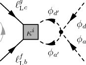
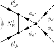
We now discuss the running due to the terms in the $\beta$ -functions with a flavour structure proportional to the unit matrix. Below and above the see-saw scales, they only cause a common scaling of the elements of the neutrino mass matrix and thus leave the mixing angles and phases unchanged. Between the thresholds, however, the effective neutrino mass matrix consists of the two parts $\accentset{(n)}{\kappa}$ and $2\,\accentset{(n)}{Y}_{\nu}^{T}\accentset{(n)}{M}^{-1}\accentset{(n)}{Y}_{\nu}$ , as shown in Eq. (12). Here, the mixing angles and phases change in general, unless both parts are scaled equally. From table 1, we see that in the SM, the $\beta$ -functions $\accentset{(n)}{\beta}_{{\kappa}}$ and $\accentset{(n)}{\beta}_{2{Y}_{\nu}^{T}{M}^{-1}{Y}_{\nu}}$ , have different coefficients in the terms proportional to the gauge couplings and to the Higgs self-coupling [27]. This difference can be understood by looking at the corresponding diagrams of the “full” and the effective theory. For instance, the diagram for the correction to the effective vertex proportional to $\lambda$ and its counterpart with the heavy singlet running in the loop are shown in figure 3. Diagram (a) is UV divergent, whereas diagram (b) is UV finite. We thus get no contribution proportional to $\lambda$ for the $\beta$ -function of the composite operator. The situation is similar for some of the diagrams corresponding to the vertex corrections proportional to the gauge couplings. Thus, in the SM, the RG scaling of the two parts $\accentset{(n)}{\kappa}$ and $2\,\accentset{(n)}{Y}_{\nu}^{T}\accentset{(n)}{M}^{-1}\accentset{(n)}{Y}_{\nu}$ of the effective mass matrix between the thresholds, caused by the interactions with trivial flavour structure, is different. This implies a running of the mixing angles and CP phases in addition to the running of the mass eigenvalues.¹¹¹¹ 11 To see this, let us assume that $U^{T}\raise 1.5pt\hbox{$\displaystyle\bigl($}\,\accentset{(n)}{\kappa}+2\,\accentset{(n)}{Y}_{\nu}^{T}\accentset{(n)}{M}^{-1}\accentset{(n)}{Y}_{\nu}\raise 1.5pt\hbox{$\displaystyle\bigr)$}\,U$ is diagonal. Then $U^{T}\raise 1.5pt\hbox{$\displaystyle\bigl($}a\,\accentset{(n)}{\kappa}+b\,2\,\accentset{(n)}{Y}_{\nu}^{T}\accentset{(n)}{M}^{-1}\accentset{(n)}{Y}_{\nu}\raise 1.5pt\hbox{$\displaystyle\bigr)$}\,U$ is in general only diagonal if $a=b$ (common scaling). This effect can even give the dominant contribution to the running of the mixing angles, as for instance in the example shown in figure 4 (from [11]).

Due to the non-renormalization theorem in supersymmetric theories, $\accentset{(n)}{\beta}_{\kappa}$ and $\accentset{(n)}{\beta}_{2Y_{\nu}^{T}M^{-1}Y_{\nu}}$ are identical in the MSSM (see Tab. 1 on p. 1), so that we can use the RGEs of Sec. 3 between the see-saw scales as well. In particular, the enhanced running between the thresholds due to terms with a trivial flavour structure does not occur. Of course, the heavy degrees of freedom have to be integrated out first, i.e. all parameters have to be replaced by the effective ones between the thresholds.

5 Mathematica Packages for Numerical RG Analyses

5.1 Numerical Solution of the RGEs

The Mathematica package \hrefhttp://www.ph.tum.de/ rge/REAP (Renormalization Group Evolution of Angles and Phases) numerically solves the RGEs of the quantities relevant for neutrino masses, for example the dimension 5 neutrino mass operator, the Yukawa matrices and the gauge couplings. The $\beta$ -functions for the SM, the MSSM and two Higgs doublet models with $\mathbb{Z}_{2}$ symmetry for FCNC suppression (2HDM) with and without right-handed neutrinos are implemented. In addition, the same models are available for Dirac neutrinos. New models can be added by the user. The heavy singlet neutrinos can be integrated out automatically at the correct mass thresholds, as described in Sec. 2.¹²¹² 12 We do not consider SUSY threshold corrections [47], as they are usually numerically less important [48]. The software can also be applied to type II see-saw models as long as one only considers the energy region below the additional see-saw scale $M_{\Delta}$ , where the new physics such as Higgs triplets only leads to another contribution to the effective neutrino mass operator. The package can be downloaded from http://www.ph.tum.de/~rge/REAP/. Mathematica 5 is required.

5.2 Extraction of Mixing Parameters from Mass Matrices

The package \hrefhttp://www.ph.tum.de/ rge/MixingParameterTools (\hrefhttp://www.ph.tum.de/ rge/MPT) allows to extract the physical lepton masses, mixing angles and CP phases from the mass matrices of the neutrinos and the charged leptons. Thus, the running of the neutrino mass matrix calculated by \hrefhttp://www.ph.tum.de/ rge/REAP can be translated into the running of the mixing parameters and the mass eigenvalues. For the definition of the mixing parameters, see App. A.1 and the documentation of the package. \hrefhttp://www.ph.tum.de/ rge/MixingParameterTools can also be useful as a stand-alone application in order to study textures without running, and it is not bound to the analysis of neutrino masses only but may be used for quark and superpartner mass matrices as well. Therefore, it can be obtained separately from \hrefhttp://www.ph.tum.de/ rge/REAP at http://www.ph.tum.de/~rge/MPT/.

5.3 Example Calculation

The following simple example demonstrates how to use the Mathematica packages to calculate the RG evolution of the neutrino mass matrix in the MSSM extended by three heavy singlet neutrinos. Of course, further documentation is provided together with the packages.

1.
The package corresponding to the model at the highest energy has to be loaded. All other packages needed in the course of the calculation are loaded automatically. (Note that ‘ is the backquote, which is used in opening quotation marks, for example.)
```
  Needs["REAP‘RGEMSSM‘"]
```
2.
Next, we specify that we would like to use the MSSM with singlet neutrinos and $\tan\beta=50$ . Furthermore, we set the SUSY breaking scale to $200\,\mathrm{GeV}$ and use the SM as an effective theory below this scale.
```
  RGEAdd["MSSM",RGEtan\[Beta]->50]
  RGEAdd["SM",RGECutoff->200]
```
3.
Now we have to provide the initial values. For instance, let us set the GUT-scale value of $\theta_{12}$ to $45^{\circ}$ and that of the first Majorana phase to $50^{\circ}$ . Besides, we use a simple diagonal pattern for the neutrino Yukawa matrix and the default values of the package for the remaining parameters.
```
  RGESetInitial[2*10^16,
    RGE\[Theta]12->45 Degree,RGE\[Phi]1->50 Degree,
    RGEY\[Nu]->{{1,0,0},{0,0.5,0},{0,0,0.1}}]
```
4.
RGESolve[low,high] solves the RGEs between the energy scales low and high. The heavy singlets are integrated out automatically at their mass thresholds.
```
  RGESolve[100,2*10^16]
```
5.
Using RGEGetSolution[scale,quantity] we can query the value of the quantity given in the second argument at the energy given in the first one. For example, this returns the mass matrix of the light neutrinos at $100\,\mathrm{GeV}$ :
```
  MatrixForm[RGEGetSolution[100,RGEM\[Nu]]]
```
6.
To find the leptonic mass parameters, we use the function MNSParameters[ $m_{\nu}$ , $Y_{e}$ ] (which also needs the Yukawa matrix of the charged leptons). The results are given in the order $\{\{\theta_{12},\theta_{13},\theta_{23},\delta,\delta_{e},\delta_{\mu},\delta_{\tau},\varphi_{1},\varphi_{2}\},\{m_{1},m_{2},m_{3}\},\{y_{e},y_{\mu},y_{\tau}\}\}$ .
```
  MNSParameters[
    RGEGetSolution[100,RGEM\[Nu]],RGEGetSolution[100,RGEYe]]
```

Finally, we can plot the running of the mixing angles:

  Needs["Graphics‘Graphics‘"]
  mNu[x_]:=RGEGetSolution[x,RGEM\[Nu]]
  Ye[x_]:=RGEGetSolution[x,RGEYe]
  \[Theta]12[x_]:=MNSParameters[mNu[x],Ye[x]][[1,1]]
  \[Theta]13[x_]:=MNSParameters[mNu[x],Ye[x]][[1,2]]
  \[Theta]23[x_]:=MNSParameters[mNu[x],Ye[x]][[1,3]]
  LogLinearPlot[{\[Theta]12[x],\[Theta]13[x],\[Theta]23[x]},
   {x,100,2*10^16}]

6 Applications

We now apply the analytical and numerical tools described in the previous sections to some specific cases with interesting RG effects above, between and below the see-saw scales within the conventional see-saw scenario.

6.1 RG Effects for a Dominant $\boldsymbol{(Y_{\nu})_{33}}$

Many unified models relate the Yukawa couplings of the different charged fermions and the neutrinos, e.g. $Y_{\nu}\sim Y_{u}$ or $Y_{\nu}\sim Y_{e}$ . For the charged fermions, the quantities accessible through observation are $Y^{\dagger}Y$ , where $Y$ denotes the corresponding Yukawa matrix. It is convenient to work in the basis where $Y_{u}^{\dagger}Y_{u}$ and $Y_{e}^{\dagger}Y_{e}$ are diagonal and positive, and the diagonal entries are ordered ascendingly. In this basis, all three combinations $Y^{\dagger}Y$ have a dominant 33 entry. In this subsection, we shall assume a similar pattern for $Y_{\nu}^{\dagger}Y_{\nu}$ , i.e. $(Y_{\nu}^{\dagger}Y_{\nu})_{33}\approx y_{3}^{2}\gg(Y_{\nu}^{\dagger}Y_{\nu})_{ij\neq 33}$ . Given such a hierarchy for $Y_{\nu}^{\dagger}Y_{\nu}$ , the RG corrections $\Delta\theta_{13}:=\theta_{13}(M_{\mathrm{SUSY}})-\theta_{13}(M_{\mathrm{GUT}})$ and $\Delta\theta_{23}$ can be approximated by

$\displaystyle\Delta\theta_{13}$	$\displaystyle\approx$	$\displaystyle\frac{-1}{32\pi^{2}}\left[C_{e}y_{\tau}^{2}\,\ln\Bigl(\frac{M_{\mathrm{GUT}}}{M_{\mathrm{SUSY}}}\Bigr)+C_{\nu}y_{3}^{2}\,\ln\Bigl(\frac{M_{\mathrm{GUT}}}{M_{*}}\Bigr)\right]\,\sin 2\theta_{12}\,\sin 2\theta_{23}\times$	(21)
		$\displaystyle{}\quad\times\frac{m_{3}}{\Delta m^{2}_{\mathrm{atm}}\left(1+\zeta\right)}\left[m_{1}\cos(\varphi_{1}-\delta)-\left(1+\zeta\right)m_{2}\,\cos(\varphi_{2}-\delta)-\zeta m_{3}\,\cos\delta\right]\quad\;\;\;$	(21)
$\displaystyle\Delta\theta_{23}$	$\displaystyle\approx$	$\displaystyle\frac{1}{32\pi^{2}}\left[C_{e}y_{\tau}^{2}\,\ln\Bigl(\frac{M_{\mathrm{GUT}}}{M_{\mathrm{SUSY}}}\Bigr)+C_{\nu}y_{3}^{2}\,\ln\Bigl(\frac{M_{\mathrm{GUT}}}{M_{*}}\Bigr)\right]\,\sin 2\theta_{23}\times$	(22)
		$\displaystyle{}\quad\times\frac{1}{\Delta m^{2}_{\mathrm{atm}}}\left[c_{12}^{2}\,\|m_{2}\,e^{\mathrm{i}\varphi_{2}}+m_{3}\|^{2}+s_{12}^{2}\,\frac{\|m_{1}\,e^{\mathrm{i}\varphi_{1}}+m_{3}\|^{2}}{1+\zeta}\right],$	(22)

where $M_{*}$ denotes the mass scale of the heavy neutrino(s) with the large Yukawa couplings.¹³¹³ 13 For the analytic estimates, we ignore complications due to the generically non-degenerate see-saw scales [27]. To obtain these results, we read off the RGEs from Tab. 12, and integrated them with the approximation of constant coefficients. This is reasonably accurate, since the running of $\theta_{13}$ and $\theta_{23}$ is almost linear on logarithmic scales [20].¹⁴¹⁴ 14 A comparison with numerical calculations shows that this is unchanged in the presence of neutrino Yukawa couplings.

In the SM, the term proportional to $y_{\tau}^{2}$ is negligible, since the Yukawa coupling is not enhanced by $\tan\beta$ . However, the $y_{3}^{2}$ contribution can be large, and it is not suppressed for small $\tan\beta$ . Furthermore, except for $y_{3}$ and $M_{*}$ , only (the RG extrapolation of) low-energy parameters enter the expressions (21) and (22).

In the case of the solar angle, the running is strongly non-linear when the RG change is large. Then, the approximation used in the above equations does not yield reliable results. Even by integrating the RGE (assuming $\theta_{12}$ to vary but the other parameters to be constant), one arrives at an expression which does not represent an accurate approximation in many cases because of the running of $\Delta m^{2}_{\mathrm{sol}}$ . Nevertheless, an inspection of the RGE reveals several qualitative features of the running such as the damping influence of the phases, as discussed in Sec. 3.1.

The running of the Majorana phases may be regarded as encouraging for the prospects of neutrinoless double $\beta$ decay experiments: it is known that even if the mass eigenvalues are large enough to make a discovery in future experiments possible, cancellations may strongly suppress the amplitude [49]. This can directly be seen from the fact that the amplitude is governed by the effective neutrino mass

\langle m_{\nu}\rangle\,=\,\left|m_{1}\,c_{12}^{2}c_{13}^{2}\,e^{\mathrm{i}\varphi_{1}}+m_{2}\,s_{12}^{2}c_{13}^{2}\,e^{\mathrm{i}\varphi_{2}}+m_{3}\,s_{13}^{2}\,e^{2\mathrm{i}\delta}\right|\;,

(23)

which is obviously suppressed if $\varphi_{1}-\varphi_{2}$ is close to $\pi$ . However, for dominant $P_{33}$ , the difference of Majorana phases is driven away from $\pi$ at low energies due to RG effects (cf. the discussion in Sec. 3.2). This implies that cancellations tend to be avoided. Note that the contribution from $Y_{e}^{\dagger}Y_{e}$ , which persists below the see-saw scales, increases the effect [20].

6.2 Neutrino Yukawa Couplings with Two Large Entries

As another example, let us assume that the neutrino Yukawa matrix contains two dominant entries, $(Y_{\nu})_{33}\approx e^{-\mathrm{i}\gamma}(Y_{\nu})_{32}\approx y_{3}$ with an arbitrary phase $\gamma$ , as it is the case in many models where the large atmospheric mixing angle emerges from $Y_{\nu}$ in the basis where $Y_{e}$ is diagonal. Then $(Y_{\nu}^{\dagger}Y_{\nu})_{33}\approx(Y_{\nu}^{\dagger}Y_{\nu})_{22}$ , which causes a cancellation between the contributions proportional to these terms in the RGEs of $\theta_{13}$ and $\theta_{23}$ . Thus, using the same linear approximation as in Sec. 6.1, we obtain the changes

$\displaystyle\Delta\theta_{13}$	$\displaystyle\approx$	$\displaystyle\frac{-1}{32\pi^{2}}\left[C_{e}y_{\tau}^{2}\,\ln\Bigl(\frac{M_{\mathrm{GUT}}}{M_{\mathrm{SUSY}}}\Bigr)\sin 2\theta_{23}-2C_{\nu}y_{3}^{2}\cos\gamma\,\ln\Bigl(\frac{M_{\mathrm{GUT}}}{M_{*}}\Bigr)\cos 2\theta_{23}\right]\,\sin 2\theta_{12}\times$	(24)
		$\displaystyle{}\quad\times\frac{m_{3}}{\Delta m^{2}_{\mathrm{atm}}\left(1+\zeta\right)}\left[m_{1}\cos(\varphi_{1}-\delta)-\left(1+\zeta\right)m_{2}\,\cos(\varphi_{2}-\delta)-\zeta m_{3}\,\cos\delta\right]$
		$\displaystyle{}+\frac{1}{16\pi^{2}}C_{\nu}y_{3}^{2}\sin\gamma\,\ln\Bigl(\frac{M_{\mathrm{GUT}}}{M_{*}}\Bigr)\sin 2\theta_{12}\times$
		$\displaystyle{}\quad\times\frac{m_{3}}{\Delta m^{2}_{\mathrm{atm}}\left(1+\zeta\right)}\left[m_{1}\sin(\varphi_{1}-\delta)-\left(1+\zeta\right)m_{2}\,\sin(\varphi_{2}-\delta)+\zeta m_{3}\,\sin\delta\right]\quad$
$\displaystyle\Delta\theta_{23}$	$\displaystyle\approx$	$\displaystyle\frac{1}{32\pi^{2}}\left[C_{e}y_{\tau}^{2}\,\ln\Bigl(\frac{M_{\mathrm{GUT}}}{M_{\mathrm{SUSY}}}\Bigr)\sin 2\theta_{23}-2C_{\nu}y_{3}^{2}\cos\gamma\,\ln\Bigl(\frac{M_{\mathrm{GUT}}}{M_{*}}\Bigr)\cos 2\theta_{23}\right]\times$	(25)
		$\displaystyle{}\quad\times\frac{1}{\Delta m^{2}_{\mathrm{atm}}}\left[c_{12}^{2}\,\|m_{2}\,e^{\mathrm{i}\varphi_{2}}+m_{3}\|^{2}+s_{12}^{2}\,\frac{\|m_{1}\,e^{\mathrm{i}\varphi_{1}}+m_{3}\|^{2}}{1+\zeta}\right]$
		$\displaystyle{}-\frac{1}{8\pi^{2}}C_{\nu}y_{3}^{2}\sin\gamma\,\ln\Bigl(\frac{M_{\mathrm{GUT}}}{M_{*}}\Bigr)\,\frac{m_{3}}{\Delta m^{2}_{\mathrm{atm}}}\left[c_{12}^{2}\,m_{2}\,\sin\varphi_{2}+s_{12}^{2}\frac{m_{1}\sin\varphi_{1}}{1+\zeta}\right]$
		$\displaystyle{}+\frac{1}{16\pi^{2}}D_{\nu}y_{3}^{2}\cos\gamma\,\ln\Bigl(\frac{M_{\mathrm{GUT}}}{M_{*}}\Bigr)\;.$

The change proportional to the real part of $P_{32}$ vanishes for maximal atmospheric mixing. Hence, the neutrino Yukawa couplings only contribute significantly to the running of $\theta_{13}$ in this case, if $(Y_{\nu})_{32}$ has a large imaginary part and if the CP phases are not close to 0 or $\pi$ . In $\Delta\theta_{23}$ , they always play a role by inducing off-diagonal elements in $Y_{e}^{\dagger}Y_{e}$ , which leads to the last term in Eq. (25). This term is actually dominant in the case of CP conservation and small $\tan\beta$ .

6.3 RG Corrections and Precision Measurements

In this section, we will estimate the order of magnitude of RG effects in see-saw models and compare it to the precision of future measurements of neutrino mixing (see also [21, 19, 50, 51] for related works). We shall first consider the effects of a large $P_{33}$ as an example. For instance, $P_{33}$ can be generated from the entry $(Y_{\nu})_{33}$ . Note that this is only an example. RG effects from different structures of $Y_{\nu}$ can be understood and estimated using the analytic formulae of Sec. 3. Graphically, the RG corrections caused by $P_{33}$ in the MSSM with $\tan\beta=20$ are illustrated in Fig. 5. We have assumed the initial values $\theta_{13}=0$ , $\theta_{23}=\pi/4$ and $\theta_{12}+\theta_{\mathrm{C}}=\pi/4$ (where $\theta_{\mathrm{C}}$ is the Cabibbo angle) at high energy, which may be especially interesting from a theoretical point of view [52, 53, 54]. The changes of $\theta_{13}$ and $\theta_{23}$ have been calculated from the approximations (21) and (22). We would like to stress that the mass squared differences are running quantities as well and taking them as constant, as it was done in Eqs. (21) and (22), restricts the accuracy of the estimates. For producing the plots in Fig. 5, we have used the values of $\Delta m^{2}_{\mathrm{atm}}$ and $\Delta m^{2}_{\mathrm{sol}}$ at $\mu=10^{14}\,\mathrm{GeV}$ . For the considered parameter ranges and for $m_{t}(m_{t})=175\,\mathrm{GeV}$ and $M_{\mathrm{SUSY}}=1\,\mathrm{TeV}$ , the mass squared differences at $\mu=10^{14}\,\mathrm{GeV}$ are about a factor $1.75$ larger than the low-energy values. Note that their running depends sensitively on the value of the top mass and on the SUSY breaking scale. The change of $\theta_{12}$ has also been determined assuming a linear running, which is possible here because only rather small neutrino masses and a moderate value of $\tan\beta$ are considered in the plot. We have used those values for the Majorana phases that do not damp the RG evolution, as well as best-fit values for the oscillation parameters. For the see-saw scale associated with the large Yukawa coupling, we have used the approximation

M_{*}\approx M_{33}\approx\frac{v^{2}}{2}(Y_{\nu})_{33}^{2}\,(m_{\nu}^{-1})_{33}\;.

(26)

To justify this, let us reconstruct $M$ from $Y_{\nu}$ and $m_{\nu}$ using the inverse of the see-saw formula (3), $M=-\frac{v^{2}}{2}Y_{\nu}\,m_{\nu}^{-1}Y_{\nu}^{T}$ , for a dominant entry $(Y_{\nu})_{33}$ in $Y_{\nu}$ and not too large neutrino masses, $m_{1}\lesssim 0.1\,\mathrm{eV}$ . In this case, one can see from $m_{\nu}^{-1}=U_{\nu}\,\diag(m_{1}^{-1},m_{2}^{-1},m_{3}^{-1})\,U_{\nu}^{T}$ that all entries of the inverse light neutrino mass matrix are usually of the same order of magnitude.¹⁵¹⁵ 15 Only for a narrow range in $m_{1}$ and a large difference of the Majorana phases, a suppression of the element $(m_{\nu}^{-1})_{33}$ is possible. Then, Eq. (26) may not be a good approximation. Consequently, $M_{33}$ is dominated by the term proportional to $(Y_{\nu})_{33}^{2}$ , i.e. the one given in Eq. (26). Furthermore, $M_{33}$ is the dominant entry in $M$ , so that it is approximately equal to the largest eigenvalue $M_{3}=M_{*}$ .

We find that the RG changes are comparable to the sensitivities of planned precision experiments (cf. Tabs. 8 and 9) in the shaded parts of the parameter space, providing a reason to be optimistic about the potential of these experiments to find interesting results and to constrain model parameters. Compared to the change due to the charged lepton Yukawa couplings alone [20], the gray-shaded regions are expanded, since the contribution from the neutrino Yukawa couplings has the same sign in the case we considered. For a very strong mass hierarchy, we find very small RG effects in our example. One reason for this is the decrease of the enhancement factors in the RGEs, as discussed in Sec. 3.1, but this is not the main effect. What is more important is the increase of $M_{*}$ . From Eq. (26) we find that it is roughly proportional to $m_{1}^{-1}$ for a strong hierarchy, so that it becomes close to or even larger than $M_{\mathrm{GUT}}$ . Consequently, the RG effects from $(Y_{\nu})_{33}$ become negligible, and we are left with the change proportional to $y_{\tau}^{2}$ . This change is small here, since we are using a moderate value of $\tan\beta=20$ .

Current Beams D-CHOOZ T2K $+$ NuMI Reactor-II JPARC-HK NuFact-II 0.14 0.061 0.032 0.023 0.014 $10^{-3}$ $6\times 10^{-5}$

Table 8: Current and expected sensitivities for

\sin^{2}2\theta_{13}

at the 90% CL [55, 56, 57]. The entry “Beams” includes the conventional beam experiments MINOS, ICARUS and OPERA. The last entry refers to an advanced stage neutrino factory with experiments at two different baselines. The sensitivity of a first stage neutrino factory (“NuFact-I”) is similar to that of JPARC-HK. For a description of the experiments and the assumptions used in the analysis, see [55, 56, 57] and references therein. The numbers should be treated with some care, since they depend on the true values of the other oscillation parameters, in particular

\Delta m^{2}_{\mathrm{atm}}

Current Beams T2K $+$ NuMI JPARC-HK NuFact-II 0.16 0.1 0.050 0.020 0.055

Table 9: Current and expected sensitivities for

|0.5-\sin^{2}\theta_{23}|

[22]. The numbers are the minimal values required to exclude maximal mixing at the 90% CL. “Current” is the current limit from SuperKamiokande [58], “Beams” means conventional neutrino beams. See [22] and references therein for a description of the experiments and the analysis methods. As in Tab. 8, the results depend on the true values of the other oscillation parameters.

In order to demonstrate that RG corrections from $Y_{\nu}$ are not necessarily negligible for a strongly hierarchical spectrum, let us consider another example, where two elements of $Y_{\nu}$ are large. The evolution of the atmospheric mixing angle and mass squared difference is shown in Fig. 6 for $\theta_{23}=\pi/4$ at high energy in the MSSM with different values of $\tan\beta$ and a strong normal mass hierarchy. In this example, we have taken $(Y_{\nu})_{33}=(Y_{\nu})_{32}=1$ at $M_{3}$ and assumed the other entries in $Y_{\nu}$ to be small in the basis where $M$ and $Y_{e}$ are diagonal. We have furthermore assumed that the right-handed neutrino with mass $M_{3}$ dominates in the see-saw formula, as it is the case for heavy sequential dominance (HSD) [59, 60].¹⁶¹⁶ 16 RG effects in this case have been discussed numerically in [26], in agreement with our analytic results. This allows to approximately calculate $M_{3}\approx v^{2}(Y_{\nu})_{33}^{2}\,m_{3}^{-1}$ with $m_{3}\approx\sqrt{\Delta m^{2}_{\mathrm{atm}}}$ in this case, and to consider only one see-saw scale $M_{*}=M_{3}$ when discussing the running. Eq. (25) then simplifies to

\Delta\theta_{23}\approx\frac{1}{32\pi^{2}}\,y_{\tau}^{2}\,\ln\Bigl(\frac{M_{\mathrm{GUT}}}{M_{\mathrm{SUSY}}}\Bigr)\left(1+2\sqrt{\zeta}c_{12}^{2}\cos\varphi_{2}\right)+\frac{1}{16\pi^{2}}\,\ln\Bigl(\frac{M_{\mathrm{GUT}}\sqrt{\Delta m^{2}_{\mathrm{atm}}}}{v^{2}}\Bigr)\;.

(27)

The resulting change of $\theta_{23}$ is in the range of about $[1^{\circ},5^{\circ}]$ . Thus, even with a strong normal mass hierarchy, the change of the mixing angles can be within the sensitivity of future long baseline experiments. The phase $\varphi_{1}$ is irrelevant due to $m_{1}=0$ , and $\varphi_{2}$ cannot cause a significant damping as it appears together with the rather small quantity $\sqrt{\zeta}$ . In Fig. 6, it has been set to 0.

As argued in Sec. 6.2, the running of $U_{e}$ (the second term in Eq. (27)) cannot be neglected in this example, because the $U_{\nu}$ contribution is strongly suppressed due to the cancellation between the terms proportional to $P_{22}$ and $P_{33}$ and the vanishing of the term proportional to $P_{23}$ for maximal atmospheric mixing and real $Y_{\nu}$ . Even without cancellations, both contributions are generically of the same order of magnitude for hierarchical neutrino masses. Another lesson that can be learned from this example is that a complete cancellation of the running is very unlikely. Hence, we always expect RG effects to be comparable to the sensitivity of planned precision experiments if there are large Yukawa couplings and if $Y_{\nu}$ and $Y_{e}$ are not simultaneously diagonal.

6.4 Large RG Effects Despite Phases

The main new effect above the see-saw thresholds is the appearance of off-diagonal terms in the Yukawa couplings. As large off-diagonal entries in the Yukawa matrices are postulated in a lot of fermion mass models in order to explain the large lepton mixing angles, we expect an important impact on the running in many cases. As mentioned in Sec. 3.1, the effect of large imaginary entries in $P$ is especially unusual, since their coefficients in the RGEs of the mixing angles $\theta_{12}$ and $\theta_{23}$ vanish for zero Majorana phases and become maximal if the phases or their difference equal $\pi/2$ . Thus, a fast running is now also possible for large Majorana phases. A numerical example with

Y_{\nu}(M_{\mathrm{GUT}})=\begin{pmatrix}0.001&0&0\\ 0&0.01&0\\ -0.4\mathrm{i}&0&0.5\end{pmatrix}\Rightarrow Y_{\nu}^{\dagger}Y_{\nu}(M_{\mathrm{GUT}})=\begin{pmatrix}0.16&0&0.2\mathrm{i}\\ 0&0.0001&0\\ -0.2\mathrm{i}&0&0.25\end{pmatrix},

(28)

i.e. a large and purely imaginary $P_{31}$ (as usual given in the basis where $Y_{e}$ is diagonal and all unphysical phases are zero) is shown in Fig. 7. We used the MSSM with $\tan\beta=30$ , $M_{\mathrm{SUSY}}=1\,\mathrm{TeV}$ , a normal hierarchy, $m_{1}=0.08\,\mathrm{eV}$ , $\Delta m^{2}_{\mathrm{sol}}=1.2\cdot 10^{-4}\,\mathrm{eV}^{2}$ , $\Delta m^{2}_{\mathrm{atm}}=4\cdot 10^{-3}\,\mathrm{eV}^{2}$ , $\varphi_{1}=\pi/2$ , $\varphi_{2}=0$ and bimaximal mixing at the GUT scale $M_{\mathrm{GUT}}=2\cdot 10^{16}\,\mathrm{GeV}$ .

Reasonable values for the low-energy oscillation parameters are reached, and $\Delta m^{2}_{\mathrm{sol}}$ stays positive. The running of the solar angle from maximal mixing to smaller values is caused by the term proportional to $\im P_{31}$ in the RGE. A negative value of $\im P_{31}$ is required for $\dot{\theta}_{12}>0$ (cf. Tab. 12), which is necessary to avoid running to the “dark side” of the solar oscillation parameters (corresponding to $\Delta m^{2}_{\mathrm{sol}}<0$ with our conventions). Alternatively, one could choose $\im P_{31}>0$ and exchange the initial phases, i.e. $\varphi_{1}=0$ , $\varphi_{2}=\pi/2$ . The terms proportional to the diagonal elements $P_{11}$ and $P_{33}$ do not play a significant role here, since they have opposite signs and therefore cancel approximately. The example demonstrates that for sufficiently large off-diagonal entries in $Y_{\nu}^{\dagger}Y_{\nu}$ , it is possible to avoid the requirement of an inverse hierarchy of the neutrino Yukawa couplings which was found for diagonal $Y_{\nu}^{\dagger}Y_{\nu}$ [11, 12, 13].

Adding another large imaginary entry in the 32-element,

Y_{\nu}(M_{\mathrm{GUT}})=\begin{pmatrix}0.001&0&0\\ 0&0.01&0\\ -0.4\mathrm{i}&-0.5\mathrm{i}&0.5\end{pmatrix}\Rightarrow Y_{\nu}^{\dagger}Y_{\nu}(M_{\mathrm{GUT}})=\begin{pmatrix}0.16&0.2&0.2\mathrm{i}\\ 0.2&0.25&0.25\mathrm{i}\\ -0.2\mathrm{i}&-0.25\mathrm{i}&0.25\end{pmatrix},

(29)

yields a rather extreme behavior of $\theta_{12}$ , as shown in Fig. 8.

The highest see-saw scale lies at about $8\cdot 10^{13}\,\mathrm{GeV}$ here, i.e. the turnaround in the running is not a threshold effect. Instead, it is due to the evolution of the Majorana phases, c.f. the lower plot in Fig. 8. Their difference initially equals $\pi/2$ but quickly starts to increase as soon as $\theta_{12}$ has moved away from $\pi/4$ . The evolution is dominated by the term proportional to $\im P_{31}$ , which is largest for $\varphi_{1}-\varphi_{2}=\pi$ . At this point, $\sin(\varphi_{1}-\varphi_{2})$ changes its sign, causing a sign change in the contributions of the imaginary parts of the off-diagonal Yukawa couplings to the RGE for $\theta_{12}$ . This explains the minimum in the evolution of this angle. At lower energies, the difference of the Majorana phases reaches a value of about $4.4$ and remains approximately constant afterwards.¹⁷¹⁷ 17 This happens even if the heaviest singlet neutrino is not integrated out, i.e. even if the large Yukawa couplings are not removed from the theory. From Tab. 14, one would expect this value to be closer to $2\pi$ . The difference is due to the subleading contributions to the running (the terms proportional to $\sin\theta_{13}$ and the charged lepton contribution), which become relevant here because of the strong damping of the leading terms.

6.5 Leptogenesis and RG Corrections

Leptogenesis [61] is an attractive explanation of the observed baryon-to-photon ratio $n_{\mathrm{B}}/n_{\gamma}=(6.5^{+0.4}_{-0.3})\cdot 10^{-10}$ [62]. It typically operates at the mass scale of the lightest right-handed neutrino. In such a scenario, we have to deal with three scales: the GUT scale where the predictions for the model parameters are fixed, the scale of leptogenesis where the parameters have to be right for successful baryogenesis, and the low scale at which the parameters can be measured in experiments. In particular, one cannot use GUT scale parameters or experimental results directly in order to test the viability of leptogenesis in a given model, rather one has to take into account quantum corrections. In the energy range between the leptogenesis scale $M_{1}$ and the electroweak scale $M_{\mathrm{EW}}$ , we can consider the running of the effective neutrino mass operator. For relating the see-saw parameters at the GUT scale with the ones at $M_{1}$ , the evolution above and between the see-saw scales has to be considered.

6.5.1 Corrections to Decay Asymmetries and to the Neutrino Mass Bound

The decay asymmetry for leptogenesis in the SM [63] can be written as

\displaystyle\varepsilon_{1}\approx\frac{3}{8\pi}\frac{M_{1}}{v^{2}}\frac{1}{(Y_{\nu}Y_{\nu}^{\dagger})_{11}}\sum_{f,g}\mbox{Im}\,[(Y_{\nu})_{1f}(Y_{\nu})_{1g}(m^{*}_{\nu})_{fg}]\;,

(30)

if $M_{1}\ll M_{2},M_{3}$ . In the MSSM, it is a factor of 2 larger. In the case of a type II see-saw and for $M_{1}\ll M_{\Delta}$ , where $M_{\Delta}$ is the mass of the SU(2)_L-triplet Higgs, the decay asymmetry for type II leptogenesis via the lightest right-handed neutrino coincides with the result for the conventional see-saw [64]. In the SM or for a moderate $\tan\beta$ in the MSSM, the RG running from $M_{\mathrm{EW}}$ to $M_{1}$ leads mainly to a scaling of the neutrino mass matrix $m_{\nu}$ . Including the RG effects results in an enhancement of the decay asymmetry for leptogenesis by roughly 20% in the MSSM and 30% – 50% in the SM [65, 20]. The decay asymmetry can be calculated by the \hrefhttp://www.ph.tum.de/ rge/REAP package described in Sec. 5 as a function of energy. Thus, one can easily check if a particular high-energy model for fermion masses is able to produce a large enough asymmetry. Let us remark that also the running of the mixing angles can be very important for the calculation of the baryon asymmetry, as has been shown recently for non-thermal leptogenesis models [66].

The requirement of successful baryogenesis via thermal leptogenesis imposes constraints on fermion mass models and even places an upper bound on the mass of the light neutrinos [67]. With respect to quantum corrections to this mass bound, it turns out that there are two effects operating in opposite directions, which partially cancel each other [20, 45, 68]: on the one hand, the increase of the mass scale leads to a larger decay asymmetry compared to the one at low energies. On the other hand, it results in a stronger washout driven by Yukawa couplings. Taking into account these effects and further corrections, one finds that the upper bound on the neutrino mass scale becomes more restrictive.

6.5.2 Models for Resonant Leptogenesis and RG Corrections

As an example where the running above the lowest see-saw scale can have large effects, we consider the RG corrections to the small mass splitting $\Delta M=|M_{1}-M_{2}|$ for resonant leptogenesis [63, 69, 70, 71]. Here, the decay asymmetry is enhanced compared to Eq. (30). For resonance effects in the decay asymmetries to be maximal, a mass splitting of $\tfrac{1}{2}$ times one of the decay widths (in the MSSM)

\displaystyle\Gamma_{1}\approx\frac{M_{0}}{8\pi}(Y_{\nu}Y^{\dagger}_{\nu})_{11}\;,\quad\Gamma_{2}\approx\frac{M_{0}}{8\pi}(Y_{\nu}Y^{\dagger}_{\nu})_{22}\;,

(31)

with $M_{2}\approx M_{1}:=M_{0}$ , is required. Given a model for neutrino masses with such a small mass splitting defined at $M_{\mathrm{GUT}}$ , the decay rate can be affected significantly by the RG evolution of the mass matrix of the heavy right-handed neutrinos from $M_{\mathrm{GUT}}$ to $M_{1}\approx M_{2}$ . Resonant leptogenesis with exactly degenerate heavy singlets at $M_{\mathrm{GUT}}$ has been discussed, e.g., in [72, 73, 74]. The running of $M$ and $Y_{\nu}$ between $M_{\mathrm{GUT}}$ and $M_{1}$ , taking into account the effects between the see-saw thresholds, can be computed conveniently using the software packages presented in Sec. 5.

7 Alternative Scenarios

For the examples in Sec. 6, we have focused on the conventional see-saw mechanism in the SM and in the MSSM. We now give a brief outlook on other scenarios. Some of them are already implemented in the software packages \hrefhttp://www.ph.tum.de/ rge/REAP/\hrefhttp://www.ph.tum.de/ rge/MPT introduced in Sec. 5.

7.1 Type II See-Saw

A generalization of the conventional see-saw is the type II see-saw [75, 76, 77], where an additional contribution to the neutrino mass matrix, e.g. from an induced vev of a $\mathrm{SU}(2)_{\mathrm{L}}$ -triplet Higgs, is present. Below the additional see-saw scale given by the mass $M_{\Delta}$ of the triplet, it can be integrated out, only leaving an additional contribution to the effective neutrino mass operator. The packages \hrefhttp://www.ph.tum.de/ rge/REAP/\hrefhttp://www.ph.tum.de/ rge/MPT and the analytic formulae for the running of the neutrino parameters can thus be applied for analyzing type II see-saw scenarios below $M_{\Delta}$ . Above $M_{\Delta}$ , the RGEs are modified due to the additional interactions.

7.2 Dirac Neutrinos

At present it is not known whether the nature of neutrino masses is Dirac or Majorana. The RG evolution of Dirac neutrino masses is studied in [44]. The packages \hrefhttp://www.ph.tum.de/ rge/REAP/\hrefhttp://www.ph.tum.de/ rge/MPT can also be used in this case.

7.3 Two Higgs Models

We restrict our discussion to a class of 2HDMs where flavour changing neutral currents (FCNCs) are naturally absent [78, 79, 80]. The Yukawa couplings of the theory are given by

	$\displaystyle\mathscr{L}_{\mathrm{Yukawa}}^{\mathrm{2HDM}}$	$\displaystyle=$	$\displaystyle-\sum\limits_{i=1}^{2}\left\{z_{e}^{(i)}\,\overline{e_{\mathrm{R}}}Y_{e}^{(i)}\ell_{\mathrm{L}}\phi^{(i)\dagger}+z_{\nu}^{(i)}\,\overline{N_{\mathrm{R}}}Y_{\nu}^{(i)}\ell_{\mathrm{L}}\widetilde{\phi}^{(i)\dagger}\right.$		(32)
			$\displaystyle\left.{}\hphantom{-\sum\limits_{i=1}^{2}\left\{\right.}+z_{d}^{(i)}\,\overline{d_{\mathrm{R}}}Y_{d}^{(i)}Q_{\mathrm{L}}\phi^{(i)\dagger}+z_{u}^{(i)}\,\overline{u_{\mathrm{R}}}Y_{u}^{(i)}Q_{\mathrm{L}}\widetilde{\phi}^{(i)\dagger}\right\}+\text{h.c.}\;,$		(32)

where either $z_{f}^{(1)}$ or $z_{f}^{(2)}$ has to be zero for each $f\in\{e,\nu,d,u\}$ in order to ensure the absence of FCNCs. In order to generate masses via Yukawa couplings, $z_{f}^{(1)}=1$ for $z_{f}^{(2)}=0$ and vice versa. By convention, the right-handed charged leptons always couple to the first Higgs, i.e. $z_{e}^{(1)}=1,z_{e}^{(2)}=0$ .

It is known that in these kind of models there are (at least) two effective neutrino mass operators. Furthermore, RG effects are comparatively large, since one has both the $\tan\beta$ enhancement as well as the absence of cancellations due to the SUSY non-renormalization theorem. An analytic understanding of the RG effects is more difficult to obtain, since the two components of the effective neutrino mass matrix

m_{\nu}\,=\,-\frac{v_{1}^{2}}{4}\kappa^{(11)}-\frac{v_{2}^{2}}{4}\kappa^{(22)}

(33)

run differently. Here, more investigations are needed, which are beyond the scope of this study. With the \hrefhttp://www.ph.tum.de/ rge/REAP package, an extensive numerical analysis is possible. Recently, the RGEs in multi-Higgs models have been derived [81]. The structure of the $\beta$ -functions is very similar.

7.4 Split SUSY

Let us note that the RGEs for the effective neutrino mass operator in the SM describe the running in the framework of ‘split supersymmetry’ [82, 83] as well, except for a contribution to the flavour-trivial part of the RGE (cf. App. D.3). This implies in particular that running effects for the mixing angles are suppressed compared to the MSSM (with not too small $\tan\beta$ ). The negative $g_{2}^{2}$ contribution to the flavour-trivial part of the RGE gets replaced by a positive $g_{1}^{1}$ contribution. This effect increases the running of the mass eigenvalues.

7.5 Other Alternative Sources of Neutrino Masses

If the dimension 5 neutrino mass operator does not give the leading contribution, possible alternative sources to the light neutrino masses can have interesting consequences. Neutrino masses can e.g. emerge from the Kähler potential in supersymmetric theories. It has been observed that in this case, large mixing angles can be an infrared fixed point of the renormalization group [84, 85]. In the SM, effects of additional dimension 6 operators on the running of the dimension 5 neutrino mass operator have been considered in [86].

8 Discussion and Conclusions

We have discussed the running of neutrino masses and leptonic mixing parameters in see-saw models involving singlet neutrinos. At energies above the masses of these heavy particles, their Yukawa couplings to the left-handed leptons play an important role. As they may be of order 1, they can cause significant quantum corrections. We have derived approximate renormalization group equations (RGEs) for the mixing angles, CP phases and mass eigenvalues. Due to the large number of parameters in the see-saw scenario, the details of the running strongly depend on the specific model under consideration. One is still able to obtain an extensive analytic understanding of the RG effects. It is instructive to compare the RGEs of the physical mixing parameters $\{\psi_{\ell}\}=\{\theta_{12},\theta_{32},\theta_{23},\delta,\varphi_{1},\varphi_{2}\}$ above the see-saw scales,

\mu\frac{\mathrm{d}}{\mathrm{d}\mu}\psi_{\ell}~=~\frac{f_{\ell}(m_{k},\text{phases})}{m_{i}^{2}-m_{j}^{2}}\times F_{\ell}^{(\nu)}(Y_{\nu},Y_{e},\{\psi_{\ell}\})+F_{\ell}^{(e)}(Y_{\nu},Y_{e},\{\psi_{\ell}\})

(34)

to those describing the evolution below the see-saw scales. The latter are obtained by replacing $F_{\ell}^{(\nu)}(Y_{\nu},Y_{e},\{\psi_{\ell}\})$ by $F_{\ell}(Y_{e},\{\psi_{\ell}\})$ and $F_{\ell}^{(e)}$ by zero in Eq. (34). Most importantly, the structure of the RGEs of the mixing parameters is the same above and below the see-saw scales. Hence, there are features common to the evolution above and below. For a degenerate spectrum, the first mass quotient in (34) becomes large, yielding strong RG effects. There are, however, important differences as well. First, the dimensionless function $F_{\ell}(Y_{e},\{\psi_{\ell}\})$ vanishes for zero mixing, which is not the case for $F_{\ell}^{(\nu)}(Y_{\nu},Y_{e},\{\psi_{\ell}\})$ . Zero mixing angles are hence not stable under the RG in the full see-saw framework. Second, in the SM or the MSSM with small $\tan\beta$ , RG effects are small below the see-saw scales. In contrast, above the entries of $Y_{\nu}$ can be of order one and cause important running effects. Third, the RGE contains the $F_{\ell}^{(e)}(Y_{\nu},Y_{e},\{\psi_{\ell}\})$ term, which describes the radiative rotation of $Y_{e}^{\dagger}Y_{e}$ in the presence of neutrino Yukawa couplings $Y_{\nu}$ . Finally, between the thresholds, there are important effects in non-supersymmetric theories which stem from the different scaling of different parts of the effective neutrino mass matrix.

We listed the leading order RG coefficients for the mixing parameter RGEs in extensive tables. Our results allow to obtain a qualitative understanding of generic effects such as the influence of the CP phases and that of the absolute neutrino mass scale. For example, non-zero phases often damp the running, but some terms in the RGEs are actually enhanced by them. A rough quantitative estimate of the size of the RG effects is possible as well. Although the change of the mixing angles is quite small for strongly hierarchical masses (in the case of a normal hierarchy), it turns out that often it is still comparable to the sensitivities of planned oscillation experiments. Therefore, quantum corrections should not be neglected in any study of fermion mass models if one aims at theoretical predictions whose precision matches that of the experiments. The neutrino mass eigenvalues always change significantly due to the RG evolution. This means that a model predicting precisely the measured value of $\Delta m^{2}_{\mathrm{atm}}=2.1\cdot 10^{-3}\,\mathrm{eV}^{2}$ at the GUT scale would actually be excluded by several standard deviations. Another consequence is a correction to the mass bound from thermal leptogenesis. Furthermore, the running of the masses of the singlet neutrinos is important for models of resonant leptogenesis.

In order to obtain precise quantitative results, the complete system of coupled RGEs has to be solved. Therefore, one has to resort to numerical calculations. For this purpose, we have developed a set of Mathematica packages, which are available at the web page http://www.ph.tum.de/~rge/. The package \hrefhttp://www.ph.tum.de/ rge/REAP solves the RGEs and thus provides the neutrino mass matrix as well as the other parameters such as Yukawa couplings at each energy. In models with heavy singlet neutrinos, they are integrated out automatically at the corresponding mass thresholds. Thus, the effects of non-degenerate singlet masses, which are generally sizable, are correctly taken into account. From the results of \hrefhttp://www.ph.tum.de/ rge/REAP, \hrefhttp://www.ph.tum.de/ rge/MixingParameterTools allows to extract the values of the mixing angles, phases and mass eigenvalues.

Acknowledgements

We would like to thank W. Buchmüller, K. Hamaguchi, F.R. Joaquim, S.F. King, M. Plümacher, P. Ramond, K. Turzyński and S. West for useful discussions. One of us (M.R.) would like to thank the Aspen Center for Physics for support. This work was partially supported by the EU 6th Framework Program MRTN-CT-2004-503369 “Quest for Unification”, MRTN-CT-2004-005104 “ForcesUniverse”, by the PPARC grant PPA/G/O/2002/ 00468, by the “Impuls- und Vernetzungsfonds” of the Helmholtz Association, contract number VH-NG-006, and by the “Sonderforschungsbereich 375 für Astro-Teilchenphysik der Deutschen Forschungsgemeinschaft”.

Note added

We have been made aware that F. R. Joaquim is finalizing a work on similar issues.

Appendix

Appendix A Conventions for Mixing Parameters and Experimental Data

A.1 Conventions

Here, we describe our conventions concerning mixing angles and phases. For a general unitary matrix we choose the so-called standard-parametrization

\displaystyle U

\displaystyle=

\displaystyle\diag(e^{\mathrm{i}\delta_{e}},e^{\mathrm{i}\delta_{\mu}},e^{\mathrm{i}\delta_{\tau}})\cdot V\cdot\diag(e^{-\mathrm{i}\varphi_{1}/2},e^{-\mathrm{i}\varphi_{2}/2},1)

(A.1)

where

V=\left(\begin{array}[]{ccc}c_{12}c_{13}&s_{12}c_{13}&s_{13}e^{-\mathrm{i}\delta}\\ -c_{23}s_{12}-s_{23}s_{13}c_{12}e^{\mathrm{i}\delta}&c_{23}c_{12}-s_{23}s_{13}s_{12}e^{\mathrm{i}\delta}&s_{23}c_{13}\\ s_{23}s_{12}-c_{23}s_{13}c_{12}e^{\mathrm{i}\delta}&-s_{23}c_{12}-c_{23}s_{13}s_{12}e^{\mathrm{i}\delta}&c_{23}c_{13}\end{array}\right)

(A.2)

with $c_{ij}$ and $s_{ij}$ defined as $\cos\theta_{ij}$ and $\sin\theta_{ij}$ , respectively.

The MNS mixing matrix $U_{\mathrm{MNS}}$ is defined to diagonalize the effective neutrino mass matrix $m_{\nu}$ in the basis where $Y_{e}^{\dagger}Y_{e}=\diag(y_{e}^{2},y_{\mu}^{2},y_{\tau}^{2})$ ,

U_{\mathrm{MNS}}^{T}\,m_{\nu}\,U_{\mathrm{MNS}}\,=\,\diag\big(m_{1},m_{2},m_{3}\big)\;.

(A.3)

The mass eigenvalues $m_{i}$ are positive, and $m_{1}<m_{2}<m_{3}$ for a normal hierarchy or $m_{3}<m_{1}<m_{2}$ for an inverted hierarchy, respectively. For our conventions for extracting the mixing parameters from the MNS matrix, we would like to refer the reader to Ref. [20] and the documentation of the MixingParameterTools package associated with this study.

A.2 Experimental Data

An overview over the best-fit values and allowed ranges for the neutrino oscillation parameters resulting from a global fit to the experimental data [41] is given in Tab. 10.

Parameter	Best-fit value	$3\sigma$ range
$\theta_{12}$	$33.2^{\circ}$	$28.7^{\circ}\;..\;38.1^{\circ}$
$\theta_{23}$	$45.0^{\circ}$	$35.7^{\circ}\;..\;55.6^{\circ}$
$\theta_{13}$	$0^{\circ}$	$0^{\circ}\;..\;13.1^{\circ}$
$\Delta m^{2}_{\mathrm{sol}}$	$7.9\cdot 10^{-5}\,\mathrm{eV}^{2}$	$(7.1\;..\;8.9)\cdot 10^{-5}\,\mathrm{eV}^{2}$
$\|\Delta m^{2}_{\mathrm{atm}}\|$	$2.1\cdot 10^{-3}\,\mathrm{eV}^{2}$	$(1.3\;..\;3.2)\cdot 10^{-3}\,\mathrm{eV}^{2}$

Table 10: Overview of experimental results for neutrino oscillation parameters [41].

Appendix B Derivation of the Analytic Formulae

This appendix contains a couple of technical details relevant for the derivation of the analytic formulae discussed in the main part. Our derivation is based on earlier works [38, 31, 39], but differs from them by a few steps allowing to express the running of the mixing parameters by the mixing parameters themselves rather than mixing matrix elements [20] (see also [87] for real couplings).

B.1 General Strategy

In an arbitrary basis, one can define unitary matrices $U_{\nu}$ and $U_{e}$ by


$\displaystyle U_{\nu}(t)^{T}\,m_{\nu}(t)\,U_{\nu}(t)$	$\displaystyle=$	$\displaystyle\diag\bigl(m_{1}(t),m_{2}(t),m_{3}(t)\bigr)\;,$	(B.4a)
$\displaystyle U_{e}(t)^{\dagger}\,Y_{e}^{\dagger}Y_{e}(t)\,U_{e}(t)$	$\displaystyle=$	$\displaystyle\diag\bigl(y_{e}^{2}(t),y_{\mu}^{2}(t),y_{\tau}^{2}(t)\bigr)\;,$	(B.4b)

where $m_{\nu}$ is the effective light neutrino mass matrix of Eq. (3). The MNS matrix is then given by

U_{\mathrm{MNS}}(t)\,=\,U_{e}^{\dagger}(t)\,U_{\nu}(t)\;.

(B.5)

For convenience, we choose to work in a basis, called reference basis in the following, where

Y_{e}^{\dagger}Y_{e}(t_{0})\,=\,\diag\big(y_{e}^{2}(t_{0}),y_{\mu}^{2}(t_{0}),y_{\tau}^{2}(t_{0})\big)\;.

(B.6)

Obviously, $U_{e}(t_{0})=\mathbbm{1}$ and $U_{\mathrm{MNS}}(t_{0})=U_{\nu}(t_{0})$ .

Let us now consider the changes caused by changing the renormalization scale according to $t_{0}\to t_{0}+\Delta t$ (with $\Delta t$ being small). The RGE (4) for $m_{\nu}$ induces a change

	$\displaystyle m_{\nu}(t_{0}+\Delta t)$	$\displaystyle=$	$\displaystyle m_{\nu}(t_{0})+\frac{\Delta t}{16\pi^{2}}\left[P(t_{0})^{T}\,m_{\nu}(t_{0})+m_{\nu}(t_{0})\,P(t_{0})+\bar{\alpha}(t_{0})\,m_{\nu}(t_{0})\right]$		(B.7)
			$\displaystyle{}+\mathscr{O}\big((\Delta t)^{2}\big)$		(B.7)

with $P=(C_{e}\,Y_{e}^{\dagger}Y_{e}+C_{\nu}\,Y_{\nu}^{\dagger}Y_{\nu})$ in the energy region above the highest see-saw scale. We restrict our derivation to this region. As explained in Sec. 4, the results for the MSSM can also be applied between the see-saw scales after replacing $Y_{\nu}$ by $\accentset{(n)}{Y_{\nu}}$ . However, this is not possible in the SM. Due to the change of $m_{\nu}$ ,

U_{\nu}(t_{0}+\Delta t)\,=\,U_{\nu}(t_{0})+\Delta t\,U_{\nu}(t_{0})\,T+\mathscr{O}\big((\Delta t)^{2}\big)\;,

(B.8)

where $T$ is to be calculated below. This relation, however, does not give the full RG change of $U_{\mathrm{MNS}}$ , since also $Y_{e}^{\dagger}Y_{e}$ gets rotated,

	$\displaystyle Y_{e}^{\dagger}Y_{e}(t_{0}+\Delta t)$	$\displaystyle=$	$\displaystyle Y_{e}^{\dagger}Y_{e}(t_{0})+\frac{\Delta t}{16\pi^{2}}\left[F^{\dagger}(t_{0})\,Y_{e}^{\dagger}Y_{e}(t_{0})+Y_{e}^{\dagger}Y_{e}\,F(t_{0})+f(t_{0})\,Y_{e}^{\dagger}Y_{e}(t_{0})\right]$		(B.9)
			$\displaystyle{}+\mathscr{O}\big((\Delta t)^{2}\big)\;,$		(B.9)

where $F=(D_{e}\,Y_{e}^{\dagger}Y_{e}+D_{\nu}\,Y_{\nu}^{\dagger}Y_{\nu})$ and $f=2\re\alpha_{e}$ . Hence, $U_{e}(t_{0}+\Delta t)$ is different from $U_{e}(t_{0})=\mathbbm{1}$ in general,

U_{e}(t_{0}+\Delta t)\,=\,U_{e}(t_{0})+\Delta t\,U_{e}(t_{0})\,X+\mathscr{O}\big((\Delta t)^{2}\big)\;,

(B.10)

with $X$ to be calculated below.

Using Eq. (B.5) together with Eqs. (B.8) and (B.10), we thus get two contributions to the change of the MNS matrix,

U_{\mathrm{MNS}}(t_{0}+\Delta t)\,=\,U_{\mathrm{MNS}}(t_{0})+\Delta t\left[U_{\mathrm{MNS}}(t_{0})\,T+X^{\dagger}\,U_{\mathrm{MNS}}(t_{0})\right]+\mathscr{O}\big((\Delta t)^{2})\;.

(B.11)

We call them the $U_{\nu}$ and the $U_{e}$ contribution. Following the analysis of [20], this relation allows to derive RGEs for the mixing parameters.

Before going to the actual calculation, we would like to stress that to derive the mixing parameter RGEs, it is useful to work in the reference basis. The resulting equations, however, are basis-independent. Of course, if one changes the basis, one needs to transform $P$ and $F$ accordingly, which means that the tables in Sec. 3 and App. C are changed as well.

B.2 RG Corrections Induced by $\boldsymbol{P}$

This part of the derivation coincides with the one performed in [20] except for the fact that we have to deal with a non-diagonal $P$ . Rather than repeating the analysis of [20], we just summarize the results: the evolution of $U_{\nu}$ is found to be described by

U_{\nu}^{\dagger}\,\dot{U}_{\nu}=T\;,

(B.12)

where the entries of $T$ are given by


$\displaystyle 16\pi^{2}\,\im T_{ij}$	$\displaystyle=$	$\displaystyle-\frac{m_{i}-m_{j}}{m_{i}+m_{j}}\,\im P^{\prime}_{ij}\;,$	(B.13a)
$\displaystyle 16\pi^{2}\,\re T_{ij}$	$\displaystyle=$	$\displaystyle-\frac{m_{i}+m_{j}}{m_{i}-m_{j}}\,\re P^{\prime}_{ij}\;.$	(B.13b)

$m_{i}$ denote the eigenvalues of the effective neutrino mass matrix $m_{\nu}$ (cf. App. A.1), and $P^{\prime}=U_{\nu}^{\dagger}\,P\,U_{\nu}$ .

B.3 Contribution from the Running of $\boldsymbol{Y_{e}}$

Let us now derive the $U_{e}$ contribution to the RGEs stemming from the fact that $Y_{e}^{\dagger}Y_{e}$ changes its structure under the RG. To calculate the corresponding change of the MNS matrix, we only need the running of the unitary matrix $U_{e}$ which diagonalizes $Y_{e}^{\dagger}Y_{e}$ . Using Eq. (18), it is easy to check that

\displaystyle 16\pi^{2}\,\frac{\mathrm{d}}{\mathrm{d}t}Y_{e}^{\dagger}Y_{e}

\displaystyle=

\displaystyle F^{\dagger}\,Y_{e}^{\dagger}Y_{e}+Y_{e}^{\dagger}Y_{e}\,F+2\re\alpha_{e}\,Y_{e}^{\dagger}Y_{e}\;.

(B.14)

Plugging this into the inverse of Eq. (B.4b), $Y_{e}^{\dagger}Y_{e}=U_{e}\,\diag(y_{e}^{2},y_{\mu}^{2},y_{\tau}^{2})\,U_{e}^{\dagger}=:U_{e}D\,U_{e}^{\dagger}$ , we obtain

	$\displaystyle\frac{\mathrm{d}}{\mathrm{d}t}(U_{e}D\,U_{e}^{\dagger})$	$\displaystyle=$	$\displaystyle\dot{U}_{e}D\,U_{e}^{\dagger}+U_{e}D\,\dot{U}_{e}^{\dagger}+U_{e}\dot{D}\,U_{e}^{\dagger}$		(B.15)
		$\displaystyle=$	$\displaystyle\frac{1}{16\pi^{2}}\left(F^{\dagger}U_{e}D\,U_{e}^{\dagger}+U_{e}D\,U_{e}^{\dagger}F+2\re\alpha_{e}\,U_{e}D\,U_{e}^{\dagger}\right).$		(B.15)

Multiplying by $U_{e}^{\dagger}$ from the left and by $U_{e}$ from the right yields

U_{e}^{\dagger}\dot{U}_{e}D+D\,\dot{U}_{e}^{\dagger}U_{e}+\dot{D}\,=\,\frac{1}{16\pi^{2}}\left(F^{\prime\,\dagger}\,D+D\,F^{\prime}+2\re\alpha_{e}\,D\right),

(B.16)

where $F^{\prime}:=U_{e}^{\dagger}\,F\,U_{e}$ . The evolution of $U_{e}$ can be written as

\frac{\mathrm{d}}{\mathrm{d}t}U_{e}\,=\,U_{e}\,X\;,

(B.17)

where $X$ is anti-Hermitian. Inserting this relation and using the anti-Hermiticity yields

\dot{D}\,=\,\frac{1}{16\pi^{2}}\left(F^{\prime\,\dagger}\,D+D\,F^{\prime}+2\re\alpha_{e}\,D\right)-X\,D+D\,X\;.

(B.18)

By analyzing the off-diagonal parts, we find

y_{i}^{2}\,X_{ij}-X_{ij}\,y_{j}^{2}\,=\,-\frac{1}{16\pi^{2}}\left[(F^{\prime\,\dagger})_{ij}\,y_{j}^{2}+y_{i}^{2}\,F^{\prime}_{ij}\right],

(B.19)

where $y_{1}\equiv y_{e}$ etc. For Hermitian $F$ , this can be written as

16\pi^{2}\,X_{ij}\,=\,\frac{y_{j}^{2}+y_{i}^{2}}{y_{j}^{2}-y_{i}^{2}}\,F_{ij}^{\prime}\;.

(B.20)

Due to the strong hierarchy of the charged lepton Yukawa couplings, the $y_{i}$ dependent factor is approximately $\pm 1$ . The corresponding equations for the $U_{\nu}$ contribution, Eqs. (B.13), contain the light neutrino mass eigenvalues, so that a significant enhancement of $T_{ij}$ , the analogon of $X_{ij}$ , occurs for quasi-degenerate neutrino masses. In this case, we expect the $U_{e}$ contribution to give only a small correction, unless severe cancellations occur in the $U_{\nu}$ contribution. However, for a strong normal neutrino mass hierarchy, both contributions are generically of the same order of magnitude. The diagonal parts of $X$ , which only influence the evolution of the unphysical phases, remain undetermined.

B.4 Combination of both Contributions

Inserting Eqs. (B.12) and (B.17) into Eq. (B.5), we find at $t=t_{0}$ in the reference basis

\frac{\mathrm{d}}{\mathrm{d}t}U_{\mathrm{MNS}}\,=\,U_{\mathrm{MNS}}\,T+X^{\dagger}\,U_{\mathrm{MNS}}

(B.21)

U_{\mathrm{MNS}}^{\dagger}\,\dot{U}_{\mathrm{MNS}}\,=\,T-U_{\mathrm{MNS}}^{\dagger}\,X\,U_{\mathrm{MNS}}=:R_{TX}\;.

(B.22)

Note that this is a relation for $U_{\mathrm{MNS}}$ where both $X$ and $T$ depend on how we split $U_{\mathrm{MNS}}$ into $U_{e}$ and $U_{\nu}$ . Specifically, in an arbitrary basis we have

U_{\mathrm{MNS}}^{\dagger}\,\dot{U}_{\mathrm{MNS}}\,=\,U_{e}\,T\,U_{e}^{\dagger}-U_{\nu}^{\dagger}\,X\,U_{\nu}\;.

(B.23)

As both sides of the last equation are anti-Hermitian, the derivatives of the mixing parameters are found from the system of linear equations

\sum\limits_{k}A^{(k)}\,\dot{\xi}_{k}+\mathrm{i}\,S^{(k)}\,\dot{\xi}_{k}\,=\,R_{TX}\;,

(B.24)

where $\{\xi_{k}\}:=\{\theta_{12},\theta_{13},\theta_{23},\delta,\delta_{e},\delta_{\mu},\delta_{\tau},\varphi_{1},\varphi_{2}\}$ . The real matrices $A^{(k)}$ and $S^{(k)}$ are antisymmetric and symmetric, respectively. Hence, each $A^{(k)}$ has 3 characteristic elements and each $S^{(k)}$ has 6, so that we can regard Eq. (B.24) as a system of 9 linear equations,

\underbrace{\left(\begin{array}[]{ccc}A^{(1)}_{12}&\cdots&A^{(9)}_{12}\\ A^{(1)}_{13}&\cdots&A^{(9)}_{13}\\ A^{(1)}_{23}&\cdots&A^{(9)}_{23}\\ S^{(1)}_{11}&\cdots&S^{(9)}_{11}\\ S^{(1)}_{12}&\cdots&S^{(9)}_{12}\\ S^{(1)}_{13}&\cdots&S^{(9)}_{13}\\ S^{(1)}_{22}&\cdots&S^{(9)}_{22}\\ S^{(1)}_{23}&\cdots&S^{(9)}_{23}\\ S^{(1)}_{33}&\cdots&S^{(9)}_{33}\end{array}\right)}_{=:\,B}\,\underbrace{\left(\begin{array}[]{c}\dot{\theta}_{12}\\[1.13809pt] \dot{\theta}_{13}\\[1.13809pt] \dot{\theta}_{23}\\[1.13809pt] \dot{\delta}\\[1.13809pt] \dot{\delta}_{e}\\[1.13809pt] \dot{\delta}_{\mu}\\[1.13809pt] \dot{\delta}_{\tau}\\[1.13809pt] \dot{\varphi}_{1}\\[1.13809pt] \dot{\varphi}_{2}\end{array}\right)}_{=\,\dot{\xi}}=\underbrace{\left(\begin{array}[]{c}\re(R_{TX})_{12}\\[1.70717pt] \re(R_{TX})_{13}\\[1.70717pt] \re(R_{TX})_{23}\\[1.70717pt] \im(R_{TX})_{11}\\[1.70717pt] \im(R_{TX})_{12}\\[1.70717pt] \im(R_{TX})_{13}\\[1.70717pt] \im(R_{TX})_{22}\\[1.70717pt] \im(R_{TX})_{23}\\[1.70717pt] \im(R_{TX})_{33}\end{array}\right)}_{=:\,v}\;.

(B.25)

$v$ can be split into two parts,

v\,=\,v_{T}+v_{X}\;,

(B.26)

where $v_{T}$ is built from $T$ and $v_{X}$ is built from $-U_{\mathrm{MNS}}^{\dagger}\,X\,U_{\mathrm{MNS}}$ . In particular, each $\dot{\xi}_{k}$ , for instance $\dot{\theta}_{12}$ , is the sum of two contributions, one from $T$ (i.e. from the running of $m_{\nu}$ ) and one from $X$ (i.e. from the running of $Y_{e}$ ).

B.5 Comment: ‘Unphysical’ Phases

The RGEs in the full theory contain the entries of $P$ . However, the phases appearing in the off-diagonal elements of $P$ are not basis-independent, rather they can be changed by a transformation using the ‘unphysical’ phases $\delta_{e}$ , $\delta_{\mu}$ and $\delta_{\tau}$ only. To see this, let us perform (in the basis where $Y_{e}^{\dagger}Y_{e}$ is diagonal) a transformation $K$ ,

\ell_{\mathrm{L}}\,\xrightarrow{K}\,K\,\ell_{\mathrm{L}}\;,\qquad e_{\mathrm{R}}\,\xrightarrow{K}\,K\,e_{\mathrm{R}}\;,

(B.27)

where $K=\diag(e^{\mathrm{i}\phi_{1}},e^{\mathrm{i}\phi_{2}},e^{\mathrm{i}\phi_{3}})$ is a diagonal phase matrix. $Y_{e}^{\dagger}Y_{e}$ is invariant under this transformation, yet it changes the effective neutrino mass matrix according to

m_{\nu}\,\xrightarrow{K}\,K^{*}\,m_{\nu}\,K^{\dagger}\;.

(B.28)

Hence, also $U_{\mathrm{MNS}}$ gets changed under this transformation,

U_{\mathrm{MNS}}\,\xrightarrow{K}\,K\,U_{\mathrm{MNS}}\;,

(B.29)

i.e. $K$ affects the phases $\delta_{e}$ , $\delta_{\mu}$ and $\delta_{\tau}$ in the standard parametrization (A.1). Furthermore, it rotates the phases of the off-diagonal entries of $Y_{\nu}^{\dagger}Y_{\nu}$ as

Y_{\nu}^{\dagger}Y_{\nu}\,\xrightarrow{K}\,K\,Y_{\nu}^{\dagger}Y_{\nu}\,K^{\dagger}\;.

(B.30)

This shows that one has to specify both the phases $\delta_{e}$ , $\delta_{\mu}$ , $\delta_{\tau}$ and the arguments of the off-diagonal entries of $Y_{\nu}^{\dagger}Y_{\nu}$ , as one set of parameters can be traded for the other. In other words, two theories with equal $P$ but different phases $\delta_{f}$ are not equivalent. In the main text, we use the convention

\delta_{e}\,=\,\delta_{\mu}\,=\,\delta_{\tau}\,=\,0\;.

(B.31)

As a technical comment, we would like to mention that in order to diagonalize a general neutrino mass matrix $m_{\nu}$ , the parameters $\delta_{e}$ , $\delta_{\mu}$ and $\delta_{\tau}$ are needed. Only after the transformation with $K=\diag(e^{-\mathrm{i}\delta_{e}},e^{-\mathrm{i}\delta_{\mu}},e^{-\mathrm{i}\delta_{\tau}})$ , one can write the MNS matrix without $\delta_{e}$ , $\delta_{\mu}$ and $\delta_{\tau}$ . The step of going to the basis where $\delta_{e}=\delta_{\mu}=\delta_{\tau}=0$ has often not been mentioned explicitly in the literature. In this context, we would like to comment that, of course, $\delta_{e}$ , $\delta_{\mu}$ and $\delta_{\tau}$ are subject to quantum corrections with their RGEs depending on the physical parameters. $\dot{\delta}_{e}$ has a term proportional to $1/\Delta m^{2}_{\mathrm{sol}}$ whereas $\dot{\delta}_{\mu}$ and $\dot{\delta}_{\tau}$ are both proportional to $1/\Delta m^{2}_{\mathrm{atm}}$ .¹⁸¹⁸ 18 The corresponding formulae below the see-saw scales can be obtained from the web page http://www.physik.tu-muenchen.de/~mratz/AnalyticFormulae/. There, the RG evolution of the $\delta_{f}$ phases depends on the physical parameters, but the RGEs of the physical parameters are independent of the $\delta_{f}$ phases.

Appendix C RGE Coefficients

In the following, we show the RGEs for the lepton mixing parameters obtained from the derivation discussed above. We give the first order of the expansion in the small CHOOZ angle $\theta_{13}$ . We furthermore use the abbreviation $\zeta$ for the ratio of the mass squared differences, cf. Eq. (16).

The results are presented in the form of tables which list the coefficients of $P_{fg}=(C_{e}\,Y_{e}^{\dagger}Y_{e}+C_{\nu}\,Y_{\nu}^{\dagger}Y_{\nu})_{fg}$ in the RGEs. Thus, if only a single element of $P$ is dominant, the derivatives of the mixing parameters are found from the corresponding rows in the tables. Of course, if several entries of $P_{fg}$ are relevant, their contributions simply add up. While the complete RGEs are basis-independent, the table entries do depend on the choice of the basis, since $P$ is basis-dependent. We use the basis where $Y_{e}$ is diagonal and where the unphysical phases in the MNS matrix are zero.

$\mathcal{C}_{13}^{12}\,=\,\frac{m_{1}}{\Delta m_{\mathrm{sol}}^{2}\left(1+\zeta\right)}\left[\left(1+\zeta\right)m_{2}\sin\left(\varphi_{1}-\varphi_{2}\right)-\zeta m_{3}\sin\left(2\delta-\varphi_{1}\right)\right]$
$\mathcal{Q}^{\pm}_{13}\,=\,\frac{\|m_{3}\pm m_{1}e^{i\varphi_{1}}\|^{2}}{\Delta m^{2}_{\mathrm{atm}}\left(1+\zeta\right)}$	$\mathcal{S}_{13}\,=\,\frac{m_{1}m_{3}\sin\varphi_{1}}{\Delta m^{2}_{\mathrm{atm}}\left(1+\zeta\right)}$
$\mathcal{Q}^{\pm}_{23}\,=\,\frac{\|m_{3}\pm m_{2}e^{i\varphi_{2}}\|^{2}}{\Delta m^{2}_{\mathrm{atm}}}$	$\mathcal{S}_{23}\,=\,\frac{m_{2}m_{3}\sin\varphi_{2}}{\Delta m^{2}_{\mathrm{atm}}}$
$\mathcal{Q}^{\pm}_{12}\,=\,\frac{\|m_{2}e^{i\varphi_{2}}\pm m_{1}e^{i\varphi_{1}}\|^{2}}{\Delta m^{2}_{\mathrm{sol}}}$	$\mathcal{S}_{12}\,=\,\frac{m_{1}m_{2}\sin(\varphi_{1}-\varphi_{2})}{\Delta m^{2}_{\mathrm{sol}}}$
$\mathcal{A}^{\pm}_{13}\,=\,\frac{\left(m_{1}^{2}+m_{3}^{2}\right)\cos\delta\pm 2m_{1}m_{3}\cos(\delta-\varphi_{1})}{\Delta m_{\mathrm{atm}}^{2}\left(1+\zeta\right)}$	$\mathcal{B}^{\pm}_{13}\,=\,\frac{\left(m_{1}^{2}+m_{3}^{2}\right)\sin\delta\pm 2m_{1}m_{3}\sin(\delta-\varphi_{1})}{\Delta m_{\mathrm{atm}}^{2}\left(1+\zeta\right)}$
$\mathcal{A}^{\pm}_{23}\,=\,\frac{\left(m_{2}^{2}+m_{3}^{2}\right)\cos\delta\pm 2m_{2}m_{3}\cos(\delta-\varphi_{2})}{\Delta m_{\mathrm{atm}}^{2}}$	$\mathcal{B}^{\pm}_{23}\,=\,\frac{\left(m_{2}^{2}+m_{3}^{2}\right)\sin\delta\pm 2m_{2}m_{3}\sin(\delta-\varphi_{2})}{\Delta m_{\mathrm{atm}}^{2}}$
$\mathcal{C}_{13}^{23}\,=\,\frac{m_{3}}{\Delta m_{\mathrm{atm}}^{2}\left(1+\zeta\right)}\left[m_{1}\sin\left(2\delta-\varphi_{1}\right)+\left(1+\zeta\right)m_{2}\sin\varphi_{2}\right]$
$\mathcal{C}_{23}^{12}\,=\,\frac{m_{2}}{\Delta m_{\mathrm{sol}}^{2}}\left[m_{1}\sin\left(\varphi_{1}-\varphi_{2}\right)-\zeta m_{3}\sin\left(2\delta-\varphi_{2}\right)\right]$
$\mathcal{C}_{23}^{13}\,=\,\frac{m_{3}}{\Delta m_{\mathrm{atm}}^{2}\left(1+\zeta\right)}\left[m_{1}\sin\varphi_{1}+\left(1+\zeta\right)m_{2}\sin\left(2\delta-\varphi_{2}\right)\right]$
$\mathcal{D}_{1}\,=\,\frac{m_{3}}{\Delta m_{\mathrm{atm}}^{2}\left(1+\zeta\right)}\left[m_{1}\cos\left(\delta-\varphi_{1}\right)-\left(1+\zeta\right)m_{2}\cos\left(\delta-\varphi_{2}\right)\right]\sin\delta$
$\mathcal{D}_{2}\,=\,\frac{m_{3}}{\Delta m_{\mathrm{atm}}^{2}\left(1+\zeta\right)}\left[m_{1}\cos\left(2\delta-\varphi_{1}\right)-\left(1+\zeta\right)m_{2}\cos\left(2\delta-\varphi_{2}\right)+\zeta m_{3}\right]$

Table 11: Definition of the abbreviations used in Tabs. 4 and 12–14

	$32\pi^{2}\,\dot{\theta}_{12}$	$64\pi^{2}\,\dot{\theta}_{13}$	$32\pi^{2}\,\dot{\theta}_{23}$
$P_{11}$	$\mathcal{Q}^{+}_{12}\sin 2\theta_{12}$	$0$	$0$
$P_{22}$	$-\mathcal{Q}^{+}_{12}\sin 2\theta_{12}c_{23}^{2}$	$\left(\mathcal{A}^{+}_{23}-\mathcal{A}^{+}_{13}\right)\sin 2\theta_{12}\sin 2\theta_{23}$	$\left(\mathcal{Q}^{+}_{23}c_{12}^{2}+\mathcal{Q}^{+}_{13}s_{12}^{2}\right)\sin 2\theta_{23}$
$P_{33}$	$-\mathcal{Q}^{+}_{12}\sin 2\theta_{12}s_{23}^{2}$	$-\!\left(\mathcal{A}^{+}_{23}-\mathcal{A}^{+}_{13}\right)\sin 2\theta_{12}\sin 2\theta_{23}$	$-\!\left(\mathcal{Q}^{+}_{23}c_{12}^{2}+\mathcal{Q}^{+}_{13}s_{12}^{2}\right)\sin 2\theta_{23}$
$\re P_{21}$	$2\mathcal{Q}^{+}_{12}\cos 2\theta_{12}c_{23}$	$4\left(\mathcal{A}^{+}_{13}c_{12}^{2}+\mathcal{A}^{+}_{23}s_{12}^{2}\right)s_{23}$	$\left(\mathcal{Q}^{+}_{23}-\mathcal{Q}^{+}_{13}\right)\sin 2\theta_{12}s_{23}$
$\re P_{31}$	$-2\mathcal{Q}^{+}_{12}\cos 2\theta_{12}s_{23}$	$4\left(\mathcal{A}^{+}_{13}c_{12}^{2}+\mathcal{A}^{+}_{23}s_{12}^{2}\right)c_{23}$	$\left(\mathcal{Q}^{+}_{23}-\mathcal{Q}^{+}_{13}\right)\sin 2\theta_{12}c_{23}$
$\re P_{32}$	$\mathcal{Q}^{+}_{12}\sin 2\theta_{12}\sin 2\theta_{23}$	$2\!\left(\mathcal{A}^{+}_{23}-\mathcal{A}^{+}_{13}\right)\sin 2\theta_{12}\cos 2\theta_{23}$	$2\!\left(\mathcal{Q}^{+}_{23}c_{12}^{2}+\mathcal{Q}^{+}_{13}s_{12}^{2}\right)\cos 2\theta_{23}$
$\im P_{21}$	$4\mathcal{S}_{12}c_{23}$	$4\left(\mathcal{B}^{-}_{13}c_{12}^{2}+\mathcal{B}^{-}_{23}s_{12}^{2}\right)s_{23}$	$2\left(\mathcal{S}_{23}-\mathcal{S}_{13}\right)\sin 2\theta_{12}s_{23}$
$\im P_{31}$	$-4\mathcal{S}_{12}s_{23}$	$4\left(\mathcal{B}^{-}_{13}c_{12}^{2}+\mathcal{B}^{-}_{23}s_{12}^{2}\right)c_{23}$	$2\left(\mathcal{S}_{23}-\mathcal{S}_{13}\right)\sin 2\theta_{12}c_{23}$
$\im P_{32}$	$0$	$2\left(\mathcal{B}^{-}_{23}-\mathcal{B}^{-}_{13}\right)\sin 2\theta_{12}$	$4\left(\mathcal{S}_{23}c_{12}^{2}+\mathcal{S}_{13}s_{12}^{2}\right)$

Table 12: Coefficients of

P_{fg}

in the RGEs of the mixing angles

\theta_{ij}

in the limit

\theta_{13}\to 0

. The abbreviations

\mathcal{A}^{\pm}_{ij}

\mathcal{B}^{\pm}_{ij}

\mathcal{S}_{ij}

and

\mathcal{Q}_{ij}^{\pm}

depend on the mass eigenvalues and phases only, and enhance the running for a degenerate mass spectrum, since they are of the form

f_{ij}(m_{i},m_{j},\text{phases})/(m_{j}^{2}-m_{i}^{2})

. They are listed in Tab. 11.

	$64\pi^{2}\dot{\delta}^{(-1)}$
$P_{11}$	$0$
$P_{22}$	$-\left(\mathcal{B}^{+}_{23}-\mathcal{B}^{+}_{13}\right)\sin 2\theta_{12}\sin 2\theta_{23}$
$P_{33}$	$\left(\mathcal{B}^{+}_{23}-\mathcal{B}^{+}_{13}\right)\sin 2\theta_{12}\sin 2\theta_{23}$
$\re P_{21}$	$-4\left(\mathcal{B}^{+}_{13}c_{12}^{2}+\mathcal{B}^{+}_{23}s_{12}^{2}\right)s_{23}$
$\re P_{31}$	$-4\left(\mathcal{B}^{+}_{13}c_{12}^{2}+\mathcal{B}^{+}_{23}s_{12}^{2}\right)c_{23}$
$\re P_{32}$	$-2\left(\mathcal{B}^{+}_{23}-\mathcal{B}^{+}_{13}\right)\sin 2\theta_{12}\cos 2\theta_{23}$
$\im P_{21}$	$4\left(\mathcal{A}^{-}_{13}c_{12}^{2}+\mathcal{A}^{-}_{23}s_{12}^{2}\right)s_{23}$
$\im P_{31}$	$4\left(\mathcal{A}^{-}_{13}c_{12}^{2}+\mathcal{A}^{-}_{23}s_{12}^{2}\right)c_{23}$
$\im P_{32}$	$2\left(\mathcal{A}^{-}_{23}-\mathcal{A}^{-}_{13}\right)\sin 2\theta_{12}$

	$64\pi^{2}\dot{\delta}^{(0)}$
$P_{11}$	$-8\left(\left(\mathcal{C}_{13}^{23}+\mathcal{S}_{12}-\mathcal{S}_{23}\right)c_{12}^{2}+\left(\mathcal{C}_{23}^{13}+\mathcal{S}_{12}-\mathcal{S}_{13}\right)s_{12}^{2}\right)$
$P_{22}$	$8\left(\left(\left(\mathcal{S}_{12}-\mathcal{S}_{23}\right)c_{23}^{2}+\mathcal{C}_{13}^{23}s_{23}^{2}\right)c_{12}^{2}+\left(\left(\mathcal{S}_{12}-\mathcal{S}_{13}\right)c_{23}^{2}+\mathcal{C}_{23}^{13}s_{23}^{2}\right)s_{12}^{2}\right)$
$P_{33}$	$8\left(\left(\mathcal{C}_{13}^{23}c_{23}^{2}+\left(\mathcal{S}_{12}-\mathcal{S}_{23}\right)s_{23}^{2}\right)c_{12}^{2}+\left(\mathcal{C}_{23}^{13}c_{23}^{2}+\left(\mathcal{S}_{12}-\mathcal{S}_{13}\right)s_{23}^{2}\right)s_{12}^{2}\right)$
$\re P_{21}$	$-16\mathcal{S}_{12}c_{23}\cot 2\theta_{12}+4\left(2\mathcal{D}_{1}c_{23}+\left(\mathcal{S}_{23}-\mathcal{S}_{13}\right)s_{23}\tan\theta_{23}\right)\sin 2\theta_{12}$
$\re P_{31}$	$16\mathcal{S}_{12}s_{23}\cot 2\theta_{12}-4\left(2\mathcal{D}_{1}s_{23}+\left(\mathcal{S}_{23}-\mathcal{S}_{13}\right)c_{23}\cot\theta_{23}\right)\sin 2\theta_{12}$
$\re P_{32}$	$-16\left(\mathcal{S}_{23}c_{12}^{2}+\mathcal{S}_{13}s_{12}^{2}\right)\cos 2\theta_{23}\cot 2\theta_{23}-8\left(\mathcal{C}_{13}^{12}c_{12}^{2}+\mathcal{C}_{23}^{12}s_{12}^{2}\right)\sin 2\theta_{23}$
$\im P_{21}$	$-8\mathcal{Q}^{-}_{12}c_{23}\csc 2\theta_{12}-2\left(2\mathcal{D}_{2}c_{23}+\left(\mathcal{Q}^{-}_{23}-\mathcal{Q}^{-}_{13}\right)\cos 2\theta_{23}\sec\theta_{23}\right)\sin 2\theta_{12}$
$\im P_{31}$	$8\mathcal{Q}^{-}_{12}s_{23}\csc 2\theta_{12}+2\left(2\mathcal{D}_{2}s_{23}-\left(\mathcal{Q}^{-}_{23}-\mathcal{Q}^{-}_{13}\right)\cos 2\theta_{23}\csc\theta_{23}\right)\sin 2\theta_{12}$
$\im P_{32}$	$-8\left(\mathcal{Q}^{-}_{23}c_{12}^{2}+\mathcal{Q}^{-}_{13}s_{12}^{2}\right)\cot 2\theta_{23}$

Table 13: Coefficients of

P_{fg}

in the derivative of the Dirac CP phase. The complete RGE is given by

\dot{\delta}=\theta_{13}^{-1}\dot{\delta}^{(-1)}+\dot{\delta}^{(0)}+\mathscr{O}{(\theta_{13})}

. The abbreviations

\mathcal{A}^{\pm}_{ij}

\mathcal{B}^{\pm}_{ij}

\mathcal{Q}_{ij}^{\pm}

\mathcal{C}_{ij}^{kl}

and

\mathcal{D}_{i}

depend on the mass eigenvalues and phases only, and are listed in Tab. 11

	$16\pi^{2}\dot{\varphi}_{1}$
$P_{11}$	$-4\mathcal{S}_{12}c_{12}^{2}$
$P_{22}$	$4\mathcal{S}_{12}c_{12}^{2}c_{23}^{2}-4\left(\mathcal{S}_{23}c_{12}^{2}+\mathcal{S}_{13}s_{12}^{2}\right)\cos 2\theta_{23}$
$P_{33}$	$4\mathcal{S}_{12}c_{12}^{2}s_{23}^{2}+4\left(\mathcal{S}_{23}c_{12}^{2}+\mathcal{S}_{13}s_{12}^{2}\right)\cos 2\theta_{23}$
$\re P_{21}$	$-4\mathcal{S}_{12}c_{23}\cos 2\theta_{12}\cot\theta_{12}-2\left(\mathcal{S}_{23}-\mathcal{S}_{13}\right)\cos 2\theta_{23}\sec\theta_{23}\sin 2\theta_{12}$
$\re P_{31}$	$4\mathcal{S}_{12}s_{23}\cos 2\theta_{12}\cot\theta_{12}-2\left(\mathcal{S}_{23}-\mathcal{S}_{13}\right)\cos 2\theta_{23}\csc\theta_{23}\sin 2\theta_{12}$
$\re P_{32}$	$-8\left(\mathcal{S}_{23}c_{12}^{2}+\mathcal{S}_{13}s_{12}^{2}\right)\cos 2\theta_{23}\cot 2\theta_{23}-4\mathcal{S}_{12}c_{12}^{2}\sin 2\theta_{23}$
$\im P_{21}$	$-2\mathcal{Q}^{-}_{12}c_{23}\cot\theta_{12}-\left(\mathcal{Q}^{-}_{23}-\mathcal{Q}^{-}_{13}\right)\cos 2\theta_{23}\sec\theta_{23}\sin 2\theta_{12}$
$\im P_{31}$	$2\mathcal{Q}^{-}_{12}s_{23}\cot\theta_{12}-\left(\mathcal{Q}^{-}_{23}-\mathcal{Q}^{-}_{13}\right)\cos 2\theta_{23}\csc\theta_{23}\sin 2\theta_{12}$
$\im P_{32}$	$-4\left(\mathcal{Q}^{-}_{23}c_{12}^{2}+\mathcal{Q}^{-}_{13}s_{12}^{2}\right)\cot 2\theta_{23}$

	$16\pi^{2}\dot{\varphi}_{2}$
$P_{11}$	$-4\mathcal{S}_{12}s_{12}^{2}$
$P_{22}$	$4\mathcal{S}_{12}c_{23}^{2}s_{12}^{2}-4\left(\mathcal{S}_{23}c_{12}^{2}+\mathcal{S}_{13}s_{12}^{2}\right)\cos 2\theta_{23}$
$P_{33}$	$4\mathcal{S}_{12}s_{23}^{2}s_{12}^{2}+4\left(\mathcal{S}_{23}c_{12}^{2}+\mathcal{S}_{13}s_{12}^{2}\right)\cos 2\theta_{23}$
$\re P_{21}$	$-4\mathcal{S}_{12}c_{23}\cos 2\theta_{12}\tan\theta_{12}-2\left(\mathcal{S}_{23}-\mathcal{S}_{13}\right)\cos 2\theta_{23}\sec\theta_{23}\sin 2\theta_{12}$
$\re P_{31}$	$4\mathcal{S}_{12}s_{23}\cos 2\theta_{12}\tan\theta_{12}-2\left(\mathcal{S}_{23}-\mathcal{S}_{13}\right)\cos 2\theta_{23}\csc\theta_{23}\sin 2\theta_{12}$
$\re P_{32}$	$-8\left(\mathcal{S}_{23}c_{12}^{2}+\mathcal{S}_{13}s_{12}^{2}\right)\cos 2\theta_{23}\cot 2\theta_{23}-4\mathcal{S}_{12}s_{12}^{2}\sin 2\theta_{23}$
$\im P_{21}$	$-2\mathcal{Q}^{-}_{12}c_{23}\tan\theta_{12}-\left(\mathcal{Q}^{-}_{23}-\mathcal{Q}^{-}_{13}\right)\cos 2\theta_{23}\sec\theta_{23}\sin 2\theta_{12}$
$\im P_{31}$	$2\mathcal{Q}^{-}_{12}s_{23}\tan\theta_{12}-\left(\mathcal{Q}^{-}_{23}-\mathcal{Q}^{-}_{13}\right)\cos 2\theta_{23}\csc\theta_{23}\sin 2\theta_{12}$
$\im P_{32}$	$-4\left(\mathcal{Q}^{-}_{23}c_{12}^{2}+\mathcal{Q}^{-}_{13}s_{12}^{2}\right)\cot 2\theta_{23}$

Table 14: Coefficients of

P_{fg}

in the RGEs of the Majorana phases for

\theta_{13}=0

Appendix D RGEs for See-Saw Models

In order to calculate the RG evolution of the effective neutrino mass matrix, the RGEs for all the parameters of the theory have to be solved simultaneously. We therefore summarize the RGEs for the minimal see-saw extensions of the SM, of the class of 2HDMs described in Sec. 7.3, and of the MSSM. We list the MS 1-loop results in the SM and 2HDM, as well as the 2-loop RGEs for the effective neutrino mass operator, the singlet mass matrix and the Yukawa couplings in the MSSM. For further RGEs and references, see e.g. [88, 89, 90, 91]. We use the notation defined in Sec. 2. In particular, a superscript $(n)$ denotes a quantity between the $n$ th and the $(n+1)$ th mass threshold. The RGEs for the SM, 2HDM or MSSM without singlet neutrinos can be recovered by setting the neutrino Yukawa coupling to zero. In the full theories above the highest see-saw scale, the superscript $(n)$ has to be omitted.

The RGEs for the gauge couplings are well-known and not affected by the additional singlets at 1-loop order. They are given by

\displaystyle 16\pi^{2}\,\beta_{g_{A}}:=16\pi^{2}\,\mu\frac{\mathrm{d}g_{A}}{\mathrm{d}\mu}=b_{A}\,g_{A}^{3}\;,

(D.32)

with $(b_{\mathrm{SU}(3)_{\mathrm{C}}},b_{\mathrm{SU}(2)_{\mathrm{L}}},b_{\mathrm{U}(1)_{\mathrm{Y}}})=(-7,-\tfrac{19}{6},\tfrac{41}{10})$ in the SM, $(-7,-3,\tfrac{21}{5})$ in the 2HDMs and $(-3,1,\tfrac{33}{5})$ in the MSSM. For $\mathrm{U}(1)_{\mathrm{Y}}$ , we use GUT charge normalization.

D.1 The RGEs in the Extended SM

In the SM extended by singlet neutrinos, the RG evolution is governed by the $\beta$ -functions [31, 27]


$\displaystyle 16\pi^{2}\accentset{(n)}{\beta}_{\kappa}$	$\displaystyle=$	$\displaystyle-\frac{3}{2}(Y_{e}^{\dagger}Y_{e})^{T}\>\accentset{(n)}{\kappa}-\frac{3}{2}\,\accentset{(n)}{\kappa}\,(Y_{e}^{\dagger}Y_{e})+\frac{1}{2}\raise 1.5pt\hbox{$\displaystyle\bigl($}\accentset{(n)}{Y}^{\dagger}_{\nu}\accentset{(n)}{Y}_{\nu}\raise 1.5pt\hbox{$\displaystyle\bigr)$}^{T}\,\accentset{(n)}{\kappa}+\frac{1}{2}\,\accentset{(n)}{\kappa}\>\raise 1.5pt\hbox{$\displaystyle\bigl($}\accentset{(n)}{Y}^{\dagger}_{\nu}\accentset{(n)}{Y}_{\nu}\raise 1.5pt\hbox{$\displaystyle\bigr)$}$	(D.33a)
		$\displaystyle{}\vphantom{\frac{1}{2}}+2\,\Tr(Y_{e}^{\dagger}Y_{e})\,\accentset{(n)}{\kappa}+2\,\Tr\raise 1.5pt\hbox{$\displaystyle\bigl($}\accentset{(n)}{Y}^{\dagger}_{\nu}\accentset{(n)}{Y}_{\nu}\raise 1.5pt\hbox{$\displaystyle\bigr)$}\,\accentset{(n)}{\kappa}+6\,\Tr(Y_{u}^{\dagger}Y_{u})\,\accentset{(n)}{\kappa}$
		$\displaystyle{}\vphantom{\frac{1}{2}}+6\,\Tr(Y_{d}^{\dagger}Y_{d})\,\accentset{(n)}{\kappa}-3g_{2}^{2}\>\accentset{(n)}{\kappa}+\lambda\accentset{(n)}{\kappa}\;,$
$\displaystyle 16\pi^{2}\accentset{(n)}{\beta}_{M}$	$\displaystyle=$	$\displaystyle\vphantom{\frac{1}{2}}\raise 1.5pt\hbox{$\displaystyle\bigl($}\accentset{(n)}{Y}_{\nu}\accentset{(n)}{Y}^{\dagger}_{\nu}\raise 1.5pt\hbox{$\displaystyle\bigr)$}\,\accentset{(n)}{M}+\accentset{(n)}{M}\,\raise 1.5pt\hbox{$\displaystyle\bigl($}\accentset{(n)}{Y}_{\nu}\accentset{(n)}{Y}^{\dagger}_{\nu}\raise 1.5pt\hbox{$\displaystyle\bigr)$}^{T}\;,$	(D.33b)
$\displaystyle 16\pi^{2}\accentset{(n)}{\beta}_{Y_{\nu}}$	$\displaystyle=$	$\displaystyle\accentset{(n)}{Y}_{\nu}\left\{\frac{3}{2}\raise 1.5pt\hbox{$\displaystyle\bigl($}\accentset{(n)}{Y}^{\dagger}_{\nu}\accentset{(n)}{Y}_{\nu}\raise 1.5pt\hbox{$\displaystyle\bigr)$}-\frac{3}{2}(Y_{e}^{\dagger}Y_{e})+\Tr\raise 1.5pt\hbox{$\displaystyle\bigl($}\accentset{(n)}{Y}^{\dagger}_{\nu}\accentset{(n)}{Y}_{\nu}\raise 1.5pt\hbox{$\displaystyle\bigr)$}+\Tr(Y_{e}^{\dagger}Y_{e})\right.$	(D.33c)
		$\displaystyle\hphantom{\accentset{(n)}{Y}_\nu\left[ \right.}\left.{}+3\,\Tr(Y_{u}^{\dagger}Y_{u})+3\,\Tr(Y_{d}^{\dagger}Y_{d})-\frac{9}{20}g_{1}^{2}-\frac{9}{4}g_{2}^{2}\right\},$	(D.33c)
$\displaystyle 16\pi^{2}\,\accentset{(n)}{\beta}_{Y_{e}}$	$\displaystyle=$	$\displaystyle Y_{e}\left\{\vphantom{\Tr\left[Y_{e}^{\dagger}Y_{e}+z_{\nu}^{(1)}\,\accentset{(n)}{Y}_{\nu}^{\dagger}\accentset{(n)}{Y}_{\nu}+3z_{d}^{(1)}\,Y_{d}^{\dagger}Y_{d}\ +3z_{u}^{(1)}\,Y_{u}^{\dagger}Y_{u}\right]}\frac{3}{2}Y_{e}^{\dagger}Y_{e}-\frac{3}{2}\,\accentset{(n)}{Y}_{\nu}^{\dagger}\accentset{(n)}{Y}_{\nu}-\frac{9}{4}g_{1}^{2}-\frac{9}{4}g_{2}^{2}\right.$	(D.33d)
		$\displaystyle\hphantom{Y_e\left\{ \right.}\left.{}+\Tr\left[Y_{e}^{\dagger}Y_{e}+\accentset{(n)}{Y}_{\nu}^{\dagger}\accentset{(n)}{Y}_{\nu}+3\,Y_{d}^{\dagger}Y_{d}\ +3\,Y_{u}^{\dagger}Y_{u}\right]\right\},$	(D.33d)
$\displaystyle 16\pi^{2}\,\accentset{(n)}{\beta}_{Y_{d}}$	$\displaystyle=$	$\displaystyle Y_{d}\left\{\frac{3}{2}Y_{d}^{\dagger}Y_{d}-\frac{3}{2}\,Y_{u}^{\dagger}Y_{u}-\frac{1}{4}g_{1}^{2}-\frac{9}{4}g_{2}^{2}-8\,g_{3}^{2}\right.$	(D.33e)
		$\displaystyle\hphantom{Y_e\left\{ \right.}\left.{}+\Tr\left[Y_{e}^{\dagger}Y_{e}+\accentset{(n)}{Y}_{\nu}^{\dagger}\accentset{(n)}{Y}_{\nu}+3\,Y_{d}^{\dagger}Y_{d}+3\,Y_{u}^{\dagger}Y_{u}\right]\right\},$	(D.33e)
$\displaystyle 16\pi^{2}\,\accentset{(n)}{\beta}_{Y_{u}}$	$\displaystyle=$	$\displaystyle Y_{u}\left\{\frac{3}{2}Y_{u}^{\dagger}Y_{u}-\frac{3}{2}\,Y_{d}^{\dagger}Y_{d}-\frac{17}{20}g_{1}^{2}-\frac{9}{4}g_{2}^{2}-8\,g_{3}^{2}\right.$	(D.33f)
		$\displaystyle\hphantom{Y_e\left\{ \right.}\left.{}+\Tr\left[Y_{e}^{\dagger}Y_{e}+\accentset{(n)}{Y}_{\nu}^{\dagger}\accentset{(n)}{Y}_{\nu}+3\,Y_{d}^{\dagger}Y_{d}+3\,Y_{u}^{\dagger}Y_{u}\right]\right\},$	(D.33f)
$\displaystyle 16\pi^{2}\,\accentset{(n)}{\beta}_{\lambda}$	$\displaystyle=$	$\displaystyle 6\,\lambda^{2}-3\,\lambda\,\left(3g_{2}^{2}+\frac{3}{5}g_{1}^{2}\right)+3\,g_{2}^{4}+\frac{3}{2}\,\left(\frac{3}{5}g_{1}^{2}+g_{2}^{2}\right)^{2}$	(D.33g)
		$\displaystyle{}+4\,\lambda\,\Tr\left[Y_{e}^{\dagger}Y_{e}+\accentset{(n)}{Y}_{\nu}^{\dagger}\accentset{(n)}{Y}_{\nu}+3\,Y_{d}^{\dagger}Y_{d}+3\,Y_{u}^{\dagger}Y_{u}\right]$
		$\displaystyle{}-8\,\Tr\left[Y_{e}^{\dagger}Y_{e}\,Y_{e}^{\dagger}Y_{e}+\accentset{(n)}{Y}_{\nu}^{\dagger}\accentset{(n)}{Y}_{\nu}\,\accentset{(n)}{Y}_{\nu}^{\dagger}\accentset{(n)}{Y}_{\nu}+3\,Y_{d}^{\dagger}Y_{d}\,Y_{d}^{\dagger}Y_{d}+3\,Y_{u}^{\dagger}Y_{u}\,Y_{u}^{\dagger}Y_{u}\right].$

We use the convention that the Higgs self-interaction term in the Lagrangian is $-\frac{\lambda}{4}(\phi^{\dagger}\phi)^{2}$ .

D.2 The RGEs in Extended 2HDMs

Here, we list the $\beta$ -functions for the class of 2HDMs described in Sec. 7.3 [92, 32, 37]. The coefficients $z_{f}^{(i)}$ determine which fermion couples to which Higgs, cf. Eq. (32).


$\displaystyle 16\pi^{2}\accentset{(n)}{\beta}_{\kappa^{(ii)}}$	$\displaystyle=$	$\displaystyle\left(\tfrac{1}{2}-2\delta_{i1}\right)\,\left[\kappa^{(ii)}(Y_{e}^{\dagger}Y_{e})+(Y_{e}^{\dagger}Y_{e})^{T}\kappa^{(ii)}\right]+\left[z^{(i)}_{\nu}\,2\,\Tr(\accentset{(n)}{Y}_{\nu}^{\dagger}\accentset{(n)}{Y}_{\nu})\right.$	(D.34a)
		$\displaystyle{}+\left.\delta_{i1}\,2\,\Tr(Y_{e}^{\dagger}Y_{e})+z^{(i)}_{u}\,6\,\Tr(Y_{u}^{\dagger}Y_{u})+z^{(i)}_{d}\,6\,\Tr(Y_{d}^{\dagger}Y_{d})\vphantom{\accentset{(n)}{Y}_{\nu}^{\dagger}\accentset{(n)}{Y}_{\nu}}\right]\kappa^{(ii)}$
		$\displaystyle{}\vphantom{\frac{1}{2}}+\lambda_{i}\kappa^{(ii)}+\delta_{i1}\lambda_{5}^{*}\kappa^{(22)}+\delta_{i2}\lambda_{5}\kappa^{(11)}-3g_{2}^{2}\kappa^{(ii)}\;,$
$\displaystyle 16\pi^{2}\accentset{(n)}{\beta}_{M}$	$\displaystyle=$	$\displaystyle\vphantom{\frac{1}{2}}\raise 1.5pt\hbox{$\displaystyle\bigl($}\accentset{(n)}{Y}_{\nu}\accentset{(n)}{Y}^{\dagger}_{\nu}\raise 1.5pt\hbox{$\displaystyle\bigr)$}\,\accentset{(n)}{M}+\accentset{(n)}{M}\,\raise 1.5pt\hbox{$\displaystyle\bigl($}\accentset{(n)}{Y}_{\nu}\accentset{(n)}{Y}^{\dagger}_{\nu}\raise 1.5pt\hbox{$\displaystyle\bigr)$}^{T},$	(D.34b)
$\displaystyle 16\pi^{2}\accentset{(n)}{\beta}_{Y_{\nu}}$	$\displaystyle=$	$\displaystyle\vphantom{\frac{1}{2}}\accentset{(n)}{Y}_{\nu}\left\{\vphantom{\sum_{i=1}^{2}z_{\nu}^{(i)}}\frac{3}{2}\accentset{(n)}{Y}_{\nu}^{\dagger}\accentset{(n)}{Y}_{\nu}+\left(\tfrac{1}{2}-2\,z_{\nu}^{(1)}\right)\frac{3}{2}Y_{e}^{\dagger}Y_{e}-\frac{9}{20}g_{1}^{2}-\frac{9}{4}g_{2}^{2}\right.$	(D.34c)
		$\displaystyle{}\left.+\sum_{i=1}^{2}\!z_{\nu}^{(i)}\,\Tr\!\left[\delta_{i1}Y_{e}^{\dagger}Y_{e}+\accentset{(n)}{Y}_{\nu}^{\dagger}\accentset{(n)}{Y}_{\nu}+3z_{d}^{(i)}\,Y_{d}^{\dagger}Y_{d}\ +3z_{u}^{(i)}\,Y_{u}^{\dagger}Y_{u}\right]\right\},$	(D.34c)
$\displaystyle 16\pi^{2}\,\accentset{(n)}{\beta}_{Y_{e}}$	$\displaystyle=$	$\displaystyle Y_{e}\left\{\vphantom{\Tr\left[Y_{e}^{\dagger}Y_{e}+z_{\nu}^{(1)}\,\accentset{(n)}{Y}_{\nu}^{\dagger}\accentset{(n)}{Y}_{\nu}+3z_{d}^{(1)}\,Y_{d}^{\dagger}Y_{d}\ +3z_{u}^{(1)}\,Y_{u}^{\dagger}Y_{u}\right]}\frac{3}{2}Y_{e}^{\dagger}Y_{e}+\left(\tfrac{1}{2}-2\,z_{\nu}^{(1)}\right)\accentset{(n)}{Y}_{\nu}^{\dagger}\accentset{(n)}{Y}_{\nu}-\frac{9}{4}g_{1}^{2}-\frac{9}{4}g_{2}^{2}\right.$	(D.34d)
		$\displaystyle\left.+\Tr\left[Y_{e}^{\dagger}Y_{e}+z_{\nu}^{(1)}\,\accentset{(n)}{Y}_{\nu}^{\dagger}\accentset{(n)}{Y}_{\nu}+3z_{d}^{(1)}\,Y_{d}^{\dagger}Y_{d}\ +3z_{u}^{(1)}\,Y_{u}^{\dagger}Y_{u}\right]\right\}\!,$	(D.34d)
$\displaystyle 16\pi^{2}\,\accentset{(n)}{\beta}_{Y_{d}}$	$\displaystyle=$	$\displaystyle Y_{d}\left\{\vphantom{\sum_{i=1}^{2}z_{d}^{(i)}\,\Tr\left[\delta_{i1}\,Y_{e}^{\dagger}Y_{e}+z_{\nu}^{(1)}\accentset{(n)}{Y}_{\nu}^{\dagger}\accentset{(n)}{Y}_{\nu}+3\,Y_{d}^{\dagger}Y_{d}\ +3z_{u}^{(i)}\,Y_{u}^{\dagger}Y_{u}\right]}\frac{3}{2}Y_{d}^{\dagger}Y_{d}+\left(\frac{1}{2}-2\sum_{i=1}^{2}\!z_{u}^{(i)}z_{d}^{(i)}\right)Y_{u}^{\dagger}Y_{u}-\frac{1}{4}g_{1}^{2}-\frac{9}{4}g_{2}^{2}-8g_{3}^{2}\right.$	(D.34e)
		$\displaystyle\left.+\sum_{i=1}^{2}\!z_{d}^{(i)}\Tr\!\left[\delta_{i1}Y_{e}^{\dagger}Y_{e}+z_{\nu}^{(i)}\accentset{(n)}{Y}_{\nu}^{\dagger}\accentset{(n)}{Y}_{\nu}+3Y_{d}^{\dagger}Y_{d}+3z_{u}^{(i)}Y_{u}^{\dagger}Y_{u}\right]\right\},$	(D.34e)
$\displaystyle 16\pi^{2}\,\accentset{(n)}{\beta}_{Y_{u}}$	$\displaystyle=$	$\displaystyle Y_{u}\left\{\vphantom{\sum_{i=1}^{2}z_{d}^{(i)}\,\Tr\left[\delta_{i1}\,Y_{e}^{\dagger}Y_{e}+z_{\nu}^{(1)}\accentset{(n)}{Y}_{\nu}^{\dagger}\accentset{(n)}{Y}_{\nu}+3\,Y_{d}^{\dagger}Y_{d}\ +3z_{u}^{(i)}\,Y_{u}^{\dagger}Y_{u}\right]}\frac{3}{2}Y_{u}^{\dagger}Y_{u}+\left(\frac{1}{2}-2\sum_{i=1}^{2}z_{u}^{(i)}z_{d}^{(i)}\right)Y_{d}^{\dagger}Y_{d}\right.\left.-\frac{17}{20}g_{1}^{2}-\frac{9}{4}g_{2}^{2}-8g_{3}^{2}\right.$	(D.34f)
		$\displaystyle\left.+\sum_{i=1}^{2}\!z_{u}^{(i)}\Tr\!\left[\delta_{i1}Y_{e}^{\dagger}Y_{e}+z_{\nu}^{(i)}\accentset{(n)}{Y}_{\nu}^{\dagger}\accentset{(n)}{Y}_{\nu}+3z_{d}^{(i)}Y_{d}^{\dagger}Y_{d}+3Y_{u}^{\dagger}Y_{u}\right]\right\}.$	(D.34f)

For the parameters of the Higgs interaction Lagrangian, the $\beta$ -functions are [92] (Note that we use different conventions for the renormalizable Higgs couplings, as specified in [37].)


$\displaystyle 16\pi^{2}\,\accentset{(n)}{\beta}_{\lambda_{1}}$	$\displaystyle=$	$\displaystyle 6\lambda_{1}^{2}+8\lambda_{3}^{2}+6\lambda_{3}\lambda_{4}+\lambda_{5}^{2}-3\lambda_{1}\left(3g_{2}^{2}+\frac{3}{5}g_{1}^{2}\right)+3g_{2}^{4}+\frac{3}{2}\left(\frac{3}{5}g_{1}^{2}+g_{2}^{2}\right)^{2}$
		$\displaystyle{}+4\lambda_{1}\Tr\left(Y_{e}^{\dagger}Y_{e}+z_{\nu}^{(1)}\,\accentset{(n)}{Y}_{\nu}^{\dagger}\accentset{(n)}{Y}_{\nu}+3z_{d}^{(1)}\,Y_{d}^{\dagger}Y_{d}+3z_{u}^{(1)}\,Y_{u}^{\dagger}Y_{u}\right)$
		$\displaystyle{}-8\Tr\left(\!Y_{e}^{\dagger}Y_{e}Y_{e}^{\dagger}Y_{e}+z_{\nu}^{(1)}\accentset{(n)}{Y}_{\nu}^{\dagger}\accentset{(n)}{Y}_{\nu}\accentset{(n)}{Y}_{\nu}^{\dagger}\accentset{(n)}{Y}_{\nu}+3z_{d}^{(1)}Y_{d}^{\dagger}Y_{d}Y_{d}^{\dagger}Y_{d}+3z_{u}^{(1)}Y_{u}^{\dagger}Y_{u}Y_{u}^{\dagger}Y_{u}\!\right),$
$\displaystyle 16\pi^{2}\,\accentset{(n)}{\beta}_{\lambda_{2}}$	$\displaystyle=$	$\displaystyle 6\lambda_{2}^{2}+8\lambda_{3}^{2}+6\lambda_{3}\lambda_{4}+\lambda_{5}^{2}-3\lambda_{2}\left(3g_{2}^{2}+\frac{3}{5}g_{1}^{2}\right)+3g_{2}^{4}+\frac{3}{2}\left(\frac{3}{5}g_{1}^{2}+g_{2}^{2}\right)^{2}$	(D.35b)
		$\displaystyle{}+4\lambda_{2}\Tr\left(z_{\nu}^{(2)}\,\accentset{(n)}{Y}_{\nu}^{\dagger}\accentset{(n)}{Y}_{\nu}+3z_{d}^{(2)}\,Y_{d}^{\dagger}Y_{d}+3z_{u}^{(2)}\,Y_{u}^{\dagger}Y_{u}\right)$
		$\displaystyle{}-8\Tr\left(z_{\nu}^{(2)}\,\accentset{(n)}{Y}_{\nu}^{\dagger}\accentset{(n)}{Y}_{\nu}\accentset{(n)}{Y}_{\nu}^{\dagger}\accentset{(n)}{Y}_{\nu}+3z_{d}^{(2)}\,Y_{d}^{\dagger}Y_{d}Y_{d}^{\dagger}Y_{d}+3z_{u}^{(2)}\,Y_{u}^{\dagger}Y_{u}Y_{u}^{\dagger}Y_{u}\right),$
$\displaystyle 16\pi^{2}\,\accentset{(n)}{\beta}_{\lambda_{3}}$	$\displaystyle=$	$\displaystyle(\lambda_{1}+\lambda_{2})\,(3\lambda_{3}+\lambda_{4})+4\lambda_{3}^{2}+2\lambda_{4}^{2}+\frac{1}{2}\lambda_{5}^{2}-3\lambda_{3}\left(3g_{2}^{2}+\frac{3}{5}g_{1}^{2}\right)+\frac{9}{4}g_{2}^{4}$	(D.35c)
		$\displaystyle{}+\frac{27}{100}g_{1}^{4}-\frac{9}{10}g_{1}^{2}g_{2}^{2}+4\lambda_{3}\Tr\left(Y_{e}^{\dagger}Y_{e}+\accentset{(n)}{Y}_{\nu}^{\dagger}\accentset{(n)}{Y}_{\nu}+3Y_{d}^{\dagger}Y_{d}+3Y_{u}^{\dagger}Y_{u}\right)$
		$\displaystyle{}-4\Tr\left(z_{\nu}^{(2)}\,Y_{e}^{\dagger}Y_{e}\,\accentset{(n)}{Y}_{\nu}^{\dagger}\accentset{(n)}{Y}_{\nu}+3\left(z_{d}^{(1)}z_{u}^{(2)}+z_{d}^{(2)}z_{u}^{(1)}\right)Y_{d}^{\dagger}Y_{d}\,Y_{u}^{\dagger}Y_{u}\right),$
$\displaystyle 16\pi^{2}\,\accentset{(n)}{\beta}_{\lambda_{4}}$	$\displaystyle=$	$\displaystyle 2\,(\lambda_{1}+\lambda_{2})\,\lambda_{4}+4\,(2\lambda_{3}+\lambda_{4})\,\lambda_{4}+8\lambda_{5}^{2}-3\lambda_{4}\left(3g_{2}^{2}+\frac{3}{5}g_{1}^{2}\right)+\frac{9}{5}g_{1}^{2}g_{2}^{2}$	(D.35d)
		$\displaystyle{}+4\lambda_{4}\Tr\left(Y_{e}^{\dagger}Y_{e}+\accentset{(n)}{Y}_{\nu}^{\dagger}\accentset{(n)}{Y}_{\nu}+3Y_{d}^{\dagger}Y_{d}+3Y_{u}^{\dagger}Y_{u}\right)$
		$\displaystyle{}+4\Tr\left(z_{\nu}^{(2)}Y_{e}^{\dagger}Y_{e}\,\accentset{(n)}{Y}_{\nu}^{\dagger}\accentset{(n)}{Y}_{\nu}+3\left(z_{d}^{(1)}z_{u}^{(2)}+z_{d}^{(2)}z_{u}^{(1)}\right)Y_{d}^{\dagger}Y_{d}\,Y_{u}^{\dagger}Y_{u}\right),$
$\displaystyle 16\pi^{2}\,\accentset{(n)}{\beta}_{\lambda_{5}}$	$\displaystyle=$	$\displaystyle\lambda_{5}\left[\vphantom{\accentset{(n)}{Y}_{\nu}^{\dagger}\accentset{(n)}{Y}_{\nu}}\lambda_{1}+\lambda_{2}+8\lambda_{3}+12\lambda_{4}-6\left(\frac{3}{5}g_{1}^{2}+3g_{2}^{2}\right)\right.$	(D.35e)
		$\displaystyle\hphantom{\lambda_5 \left[\right.}\left.{}+2\Tr\left(Y_{e}^{\dagger}Y_{e}+\accentset{(n)}{Y}_{\nu}^{\dagger}\accentset{(n)}{Y}_{\nu}+3Y_{d}^{\dagger}Y_{d}+3Y_{u}^{\dagger}Y_{u}\right)\right].$	(D.35e)

D.3 Split Supersymmetry

The $\beta$ -functions for the renormalizable couplings in the framework of split SUSY are listed in Ref. [83]. The diagrams contributing to the RGE of the effective neutrino mass operator are those relevant in the SM, amended by two diagrams involving Higgsinos and gauginos (cf. Fig. 9). These diagrams contribute to the flavour-trivial part of the RGE.

At 1 loop, we obtain for the divergent parts of the renormalization constants in dimensional regularization and in the MS scheme


$\displaystyle\delta Z_{\phi,1}$	$\displaystyle=$	$\displaystyle-\frac{1}{16\pi^{2}}\left[2\,\Tr\left(3Y_{u}^{\dagger}Y_{u}+3Y_{d}^{\dagger}Y_{d}+Y_{e}^{\dagger}Y_{e}\right)+\frac{3}{10}(\xi_{1}-1)g_{1}^{2}+\frac{3}{2}(\xi_{2}-1)g_{2}^{2}\right],$
$\displaystyle\delta Z_{\ell_{\mathrm{L}},1}$	$\displaystyle=$	$\displaystyle-\frac{1}{16\pi^{2}}\left(Y_{e}^{\dagger}Y_{e}+\frac{3}{10}\xi_{1}\,g_{1}^{2}+\frac{3}{2}\xi_{2}\,g_{2}^{2}\right),$
$\displaystyle\delta\kappa_{,1}$	$\displaystyle=$	$\displaystyle-\frac{1}{16\pi^{2}}\left\{2\kappa\,(Y_{e}^{\dagger}Y_{e})+2(Y_{e}^{\dagger}Y_{e})^{T}\kappa-\left[\lambda+\frac{3}{5}\left(\frac{3}{2}-\xi_{1}\right)g_{1}^{2}+\left(\frac{3}{2}-3\xi_{2}\right)g_{2}^{2}\right]\kappa\right\},$

where $\xi_{1}$ and $\xi_{2}$ are the gauge parameters in $R_{\xi}$ gauge. $Z_{i}:=\mathbbm{1}+\delta Z_{i,1}\,\frac{1}{\epsilon}+\dots$ ( $\epsilon:=4-d$ ) are wavefunction renormalization constants, and $\delta\kappa:=\delta\kappa_{,1}\,\frac{1}{\epsilon}+\dots$ is defined via the counterterm for the dimension 5 operator,

\mathscr{C}_{\kappa}\,=\,\frac{1}{4}\,\delta\kappa_{fg}\;(\overline{\ell_{\mathrm{L}}^{\mathrm{C}}}{}^{f}\cdot\phi)\;(\ell_{\mathrm{L}}^{g}\cdot\phi)+\text{h.c.}\;.

Using the method described in [36], we then find the 1-loop $\beta$ -function

	$\displaystyle 16\pi^{2}\,\beta_{\kappa}^{\mathrm{Split\>SUSY}}$	$\displaystyle=$	$\displaystyle-\frac{3}{2}(Y_{e}^{\dagger}Y_{e})^{T}\kappa-\frac{3}{2}\kappa\,(Y_{e}^{\dagger}Y_{e})$		(D.37)
			$\displaystyle{}+\left[\lambda+\frac{3}{5}g_{1}^{2}+2\,\Tr\left(3Y_{u}^{\dagger}Y_{u}+3Y_{d}^{\dagger}Y_{d}+Y_{e}^{\dagger}Y_{e}\right)\right]\kappa\;.$		(D.37)

Clearly, the term involving the gauge couplings in the flavour-diagonal part differs from the SM case.

D.4 The RGEs in the MSSM Extended by Heavy Singlets

We give the 2-loop RGEs for the quantities $Q\in\left\{\accentset{(n)}{\kappa},\accentset{(n)}{M},\accentset{(n)}{Y}_{\nu},{Y}_{d},{Y}_{u},{Y}_{e}\right\}$ in the form

\mu\frac{\mathrm{d}\accentset{(n)}{Q}}{\mathrm{d}\mu}=\accentset{(n)}{\beta}_{Q}^{\,(1)}+\accentset{(n)}{\beta}_{Q}^{\,(2)}\;.

(D.38)

The 1-loop parts are given by [32, 27]


$\displaystyle(4\pi)^{2}\accentset{(n)}{\beta}^{\,(1)}_{\kappa}$	$\displaystyle=$	$\displaystyle\vphantom{\frac{1}{2}}(Y_{e}^{\dagger}Y_{e})^{T}\>\accentset{(n)}{\kappa}+\accentset{(n)}{\kappa}\,(Y_{e}^{\dagger}Y_{e})+\raise 1.5pt\hbox{$\displaystyle\bigl($}\accentset{(n)}{Y}^{\dagger}_{\nu}\accentset{(n)}{Y}_{\nu}\raise 1.5pt\hbox{$\displaystyle\bigr)$}^{T}\,\accentset{(n)}{\kappa}+\accentset{(n)}{\kappa}\>\raise 1.5pt\hbox{$\displaystyle\bigl($}\accentset{(n)}{Y}^{\dagger}_{\nu}\accentset{(n)}{Y}_{\nu}\raise 1.5pt\hbox{$\displaystyle\bigr)$}$	(D.39a)
		$\displaystyle{}+2\Tr\raise 1.5pt\hbox{$\displaystyle\bigl($}\accentset{(n)}{Y}^{\dagger}_{\nu}\accentset{(n)}{Y}_{\nu}\raise 1.5pt\hbox{$\displaystyle\bigr)$}\,\accentset{(n)}{\kappa}+6\Tr(Y_{u}^{\dagger}Y_{u})\,\accentset{(n)}{\kappa}-\frac{6}{5}g_{1}^{2}\>\accentset{(n)}{\kappa}-6g_{2}^{2}\>\accentset{(n)}{\kappa}\;,$	(D.39a)
$\displaystyle(4\pi)^{2}\accentset{(n)}{\beta}^{\,(1)}_{M}$	$\displaystyle=$	$\displaystyle\vphantom{\frac{1}{2}}2\,\raise 1.5pt\hbox{$\displaystyle\bigl($}\accentset{(n)}{Y}_{\nu}\accentset{(n)}{Y}^{\dagger}_{\nu}\raise 1.5pt\hbox{$\displaystyle\bigr)$}\,\accentset{(n)}{M}+2\,\accentset{(n)}{M}\,\raise 1.5pt\hbox{$\displaystyle\bigl($}\accentset{(n)}{Y}_{\nu}\accentset{(n)}{Y}^{\dagger}_{\nu}\raise 1.5pt\hbox{$\displaystyle\bigr)$}^{T},$	(D.39b)
$\displaystyle(4\pi)^{2}\accentset{(n)}{\beta}^{\,(1)}_{Y_{\nu}}$	$\displaystyle=$	$\displaystyle\accentset{(n)}{Y}_{\nu}\left\{3\accentset{(n)}{Y}^{\dagger}_{\nu}\accentset{(n)}{Y}_{\nu}+Y_{e}^{\dagger}Y_{e}+\Tr\raise 1.5pt\hbox{$\displaystyle\bigl($}\accentset{(n)}{Y}^{\dagger}_{\nu}\accentset{(n)}{Y}_{\nu}\raise 1.5pt\hbox{$\displaystyle\bigr)$}+3\Tr(Y_{u}^{\dagger}Y_{u})-\frac{3}{5}g_{1}^{2}-3g_{2}^{2}\right\},$	(D.39c)
$\displaystyle(4\pi)^{2}\accentset{(n)}{\beta}_{Y_{d}}^{\,(1)}$	$\displaystyle=$	$\displaystyle Y_{d}\left\{3Y_{d}^{\dagger}Y_{d}+Y_{u}^{\dagger}Y_{u}+3\Tr(Y_{d}^{\dagger}Y_{d})+\Tr(Y_{e}^{\dagger}Y_{e})-\frac{7}{15}g_{1}^{2}-3g_{2}^{2}-\frac{16}{3}g_{3}^{2}\right\},$
$\displaystyle(4\pi)^{2}\accentset{(n)}{\beta}_{Y_{u}}^{\,(1)}$	$\displaystyle=$	$\displaystyle Y_{u}\left\{Y_{d}^{\dagger}Y_{d}+3Y_{u}^{\dagger}Y_{u}+\Tr(\accentset{(n)}{Y}_{\nu}^{\dagger}\accentset{(n)}{Y}_{\nu})+3\Tr(Y_{u}^{\dagger}Y_{u})-\frac{13}{15}g_{1}^{2}-3g_{2}^{2}-\frac{16}{3}g_{3}^{2}\right\},$
$\displaystyle(4\pi)^{2}\accentset{(n)}{\beta}_{Y_{e}}^{\,(1)}$	$\displaystyle=$	$\displaystyle Y_{e}\left\{3Y_{e}^{\dagger}Y_{e}+\accentset{(n)}{Y}_{\nu}^{\dagger}\accentset{(n)}{Y}_{\nu}+3\Tr(Y_{d}^{\dagger}Y_{d})+\Tr(Y_{e}^{\dagger}Y_{e})-\frac{9}{5}g_{1}^{2}-3g_{2}^{2}\right\}.$	(D.39f)

The results for the 2-loop parts, which are an extension of the usual 2-loop $\beta$ -functions for the MSSM [93], are [94]


$\displaystyle(4\pi)^{4}\,{\accentset{(n)}{\beta}^{\,(2)}_{\kappa}}=\left[\vphantom{\frac{1}{2}}-6\Tr(Y_{u}Y_{d}^{\dagger}Y_{d}Y_{u}^{\dagger})-18\Tr(Y_{u}Y_{u}^{\dagger}Y_{u}Y_{u}^{\dagger})\right.-2\Tr(\accentset{(n)}{Y}_{\nu}Y_{e}^{\dagger}Y_{e}\accentset{(n)}{Y}_{\nu}^{\dagger})$		(D.40a)
	$\displaystyle\left.{}-6\Tr(\accentset{(n)}{Y}_{\nu}^{\dagger}\accentset{(n)}{Y}_{\nu}\accentset{(n)}{Y}_{\nu}^{\dagger}\accentset{(n)}{Y}_{\nu})+\frac{8}{5}g_{1}^{2}\Tr(Y_{u}^{\dagger}Y_{u})+32g_{3}^{2}\Tr(Y_{u}^{\dagger}Y_{u})+\frac{207}{25}g_{1}^{4}+\frac{18}{5}g_{1}^{2}g_{2}^{2}+15g_{2}^{4}\right]\accentset{(n)}{\kappa}$
	$\displaystyle{}-\left[2(Y_{e}^{\dagger}Y_{e}Y_{e}^{\dagger}Y_{e})^{T}+2(\accentset{(n)}{Y}_{\nu}^{\dagger}\accentset{(n)}{Y}_{\nu}\accentset{(n)}{Y}_{\nu}^{\dagger}\accentset{(n)}{Y}_{\nu})^{T}+\left(\Tr(\accentset{(n)}{Y}_{\nu}\accentset{(n)}{Y}_{\nu}^{\dagger})+3\Tr(Y_{u}Y_{u}^{\dagger})\right)(\accentset{(n)}{Y}_{\nu}^{\dagger}\accentset{(n)}{Y}_{\nu})^{T}\right.$
	$\displaystyle\hphantom{-\left[\vphantom{\frac{1}{2}}\right.}\left.+\left(-\frac{6}{5}g_{1}^{2}+\Tr(Y_{e}Y_{e}^{\dagger})+3\Tr(Y_{d}Y_{d}^{\dagger})\right)(Y_{e}^{\dagger}Y_{e})^{T}\right]\accentset{(n)}{\kappa}$
	$\displaystyle{}-\accentset{(n)}{\kappa}\left[2Y_{e}^{\dagger}Y_{e}Y_{e}^{\dagger}Y_{e}+2\accentset{(n)}{Y}_{\nu}^{\dagger}\accentset{(n)}{Y}_{\nu}\accentset{(n)}{Y}_{\nu}^{\dagger}\accentset{(n)}{Y}_{\nu}+\left(\Tr(\accentset{(n)}{Y}_{\nu}\accentset{(n)}{Y}_{\nu}^{\dagger})+3\Tr(Y_{u}Y_{u}^{\dagger})\right)\accentset{(n)}{Y}_{\nu}^{\dagger}\accentset{(n)}{Y}_{\nu}\right.$
	$\displaystyle\hphantom{-\accentset{(n)}{\kappa} \left[\vphantom{\frac{1}{2}}\right.}\left.+\left(-\frac{6}{5}g_{1}^{2}+\Tr(Y_{e}Y_{e}^{\dagger})+3\Tr(Y_{d}Y_{d}^{\dagger})\right)Y_{e}^{\dagger}Y_{e}\right],$
$\displaystyle(4\pi)^{4}\accentset{(n)}{\beta}_{M}^{\,(2)}=\accentset{(n)}{M}\left[\vphantom{\frac{1}{2}}-2\accentset{(n)}{Y}_{\nu}^{}Y_{e}^{T}Y_{e}^{}\accentset{(n)}{Y}_{\nu}^{T}-2\accentset{(n)}{Y}_{\nu}^{}\accentset{(n)}{Y}_{\nu}^{T}\accentset{(n)}{Y}_{\nu}^{}\accentset{(n)}{Y}_{\nu}^{T}-6\accentset{(n)}{Y}_{\nu}^{*}\accentset{(n)}{Y}_{\nu}^{T}\,\Tr(Y_{u}Y_{u}^{\dagger})\right.$		(D.40b)
	$\displaystyle{}\qquad\qquad\quad\>-2\accentset{(n)}{Y}_{\nu}^{}\accentset{(n)}{Y}_{\nu}^{T}\,\Tr(\accentset{(n)}{Y}_{\nu}\accentset{(n)}{Y}_{\nu}^{\dagger})+\frac{6}{5}g_{1}^{2}\,\accentset{(n)}{Y}_{\nu}^{}\accentset{(n)}{Y}_{\nu}^{T}+6g_{2}^{2}\,\accentset{(n)}{Y}_{\nu}^{*}\accentset{(n)}{Y}_{\nu}^{T}\left.\vphantom{\frac{1}{2}}\right]$
	$\displaystyle{}+\left[\vphantom{\frac{1}{2}}-2\accentset{(n)}{Y}_{\nu}Y_{e}^{\dagger}Y_{e}\accentset{(n)}{Y}_{\nu}^{\dagger}-2\accentset{(n)}{Y}_{\nu}\accentset{(n)}{Y}_{\nu}^{\dagger}\accentset{(n)}{Y}_{\nu}\accentset{(n)}{Y}_{\nu}^{\dagger}-6\accentset{(n)}{Y}_{\nu}\accentset{(n)}{Y}_{\nu}^{\dagger}\,\Tr(Y_{u}Y_{u}^{\dagger})-2\accentset{(n)}{Y}_{\nu}\accentset{(n)}{Y}_{\nu}^{\dagger}\,\Tr(\accentset{(n)}{Y}_{\nu}\accentset{(n)}{Y}_{\nu}^{\dagger})\right.$
	$\displaystyle{}\hphantom{+\left[\vphantom{\frac{1}{2}}\right.}+\frac{6}{5}g_{1}^{2}\,\accentset{(n)}{Y}_{\nu}\accentset{(n)}{Y}_{\nu}^{\dagger}+6g_{2}^{2}\,\accentset{(n)}{Y}_{\nu}\accentset{(n)}{Y}_{\nu}^{\dagger}\left.\vphantom{\frac{1}{2}}\right]\accentset{(n)}{M}\;,$
$\displaystyle(4\pi)^{4}\accentset{(n)}{\beta}_{Y_{\nu}}^{\,(2)}=\accentset{(n)}{Y}_{\nu}\left\{\vphantom{\frac{1}{2}}\right.-2Y_{e}^{\dagger}Y_{e}Y_{e}^{\dagger}Y_{e}-2Y_{e}^{\dagger}Y_{e}\accentset{(n)}{Y}_{\nu}^{\dagger}\accentset{(n)}{Y}_{\nu}-4\accentset{(n)}{Y}_{\nu}^{\dagger}\accentset{(n)}{Y}_{\nu}\accentset{(n)}{Y}_{\nu}^{\dagger}\accentset{(n)}{Y}_{\nu}-3Y_{e}^{\dagger}Y_{e}\Tr(Y_{d}Y_{d}^{\dagger})$
	$\displaystyle{}-Y_{e}^{\dagger}Y_{e}\Tr(Y_{e}Y_{e}^{\dagger})-3\accentset{(n)}{Y}_{\nu}^{\dagger}\accentset{(n)}{Y}_{\nu}\Tr(\accentset{(n)}{Y}_{\nu}\accentset{(n)}{Y}_{\nu}^{\dagger})-9\accentset{(n)}{Y}_{\nu}^{\dagger}\accentset{(n)}{Y}_{\nu}\Tr(Y_{u}Y_{u}^{\dagger})\vphantom{\frac{1}{2}}-\Tr(\accentset{(n)}{Y}_{\nu}Y_{e}^{\dagger}Y_{e}\accentset{(n)}{Y}_{\nu}^{\dagger})$
	$\displaystyle{}-3\Tr(\accentset{(n)}{Y}_{\nu}^{\dagger}\accentset{(n)}{Y}_{\nu}\accentset{(n)}{Y}_{\nu}^{\dagger}\accentset{(n)}{Y}_{\nu})-3\Tr(Y_{u}Y_{d}^{\dagger}Y_{d}Y_{u}^{\dagger})-9\Tr(Y_{u}Y_{u}^{\dagger}Y_{u}Y_{u}^{\dagger})\vphantom{\frac{1}{2}}+\frac{6}{5}g_{1}^{2}\,Y_{e}^{\dagger}Y_{e}+\frac{6}{5}g_{1}^{2}\,\accentset{(n)}{Y}_{\nu}^{\dagger}\accentset{(n)}{Y}_{\nu}$
	$\displaystyle{}+6g_{2}^{2}\,\accentset{(n)}{Y}_{\nu}^{\dagger}\accentset{(n)}{Y}_{\nu}+\frac{4}{5}g_{1}^{2}\,\Tr(Y_{u}^{\dagger}Y_{u})+16g_{3}^{2}\,\Tr(Y_{u}^{\dagger}Y_{u})+\frac{207}{50}g_{1}^{4}+\frac{9}{5}g_{1}^{2}g_{2}^{2}+\frac{15}{2}g_{2}^{4}\left.\vphantom{\frac{1}{2}}\right\},$
$\displaystyle(4\pi)^{4}\accentset{(n)}{\beta}_{Y_{d}}^{\,(2)}=Y_{d}\left\{\vphantom{\frac{1}{2}}-4Y_{d}^{\dagger}Y_{d}Y_{d}^{\dagger}Y_{d}-2Y_{u}^{\dagger}Y_{u}Y_{d}^{\dagger}Y_{d}-2Y_{u}^{\dagger}Y_{u}Y_{u}^{\dagger}Y_{u}-9\Tr(Y_{d}Y_{d}^{\dagger}Y_{d}Y_{d}^{\dagger})\right.$		(D.40d)
	$\displaystyle\vphantom{\frac{1}{2}}-3\Tr(Y_{d}Y_{u}^{\dagger}Y_{u}Y_{d}^{\dagger})-3\Tr(Y_{e}Y_{e}^{\dagger}Y_{e}Y_{e}^{\dagger})-\Tr(Y_{e}\accentset{(n)}{Y}_{\nu}^{\dagger}\accentset{(n)}{Y}_{\nu}Y_{e}^{\dagger})-9Y_{d}^{\dagger}Y_{d}\,\Tr(Y_{d}Y_{d}^{\dagger})$
	$\displaystyle\vphantom{\frac{1}{2}}-3Y_{d}^{\dagger}Y_{d}\,\Tr(Y_{e}Y_{e}^{\dagger})-Y_{u}^{\dagger}Y_{u}\,\Tr(\accentset{(n)}{Y}_{\nu}\accentset{(n)}{Y}_{\nu}^{\dagger})-3Y_{u}^{\dagger}Y_{u}\,\Tr(Y_{u}Y_{u}^{\dagger})+6g_{2}^{2}\,Y_{d}^{\dagger}Y_{d}$
	$\displaystyle\vphantom{\frac{1}{2}}+\frac{4}{5}g_{1}^{2}\,Y_{d}^{\dagger}Y_{d}+\frac{4}{5}g_{1}^{2}\,Y_{u}^{\dagger}Y_{u}-\frac{2}{5}g_{1}^{2}\,\Tr(Y_{d}^{\dagger}Y_{d})+\frac{6}{5}g_{1}^{2}\,\Tr(Y_{e}^{\dagger}Y_{e})+16g_{3}^{2}\,\Tr(Y_{d}^{\dagger}Y_{d})$
	$\displaystyle\vphantom{\frac{1}{2}}+\frac{287}{90}g_{1}^{4}+g_{1}^{2}g_{2}^{2}+\frac{15}{2}g_{2}^{4}+\frac{8}{9}g_{1}^{2}g_{3}^{2}+8g_{2}^{2}g_{3}^{2}-\frac{16}{9}g_{3}^{4}\left.\vphantom{\frac{1}{2}}\right\},$
$\displaystyle(4\pi)^{4}\accentset{(n)}{\beta}_{Y_{u}}^{\,(2)}=Y_{u}\left\{-2Y_{d}^{\dagger}Y_{d}Y_{d}^{\dagger}Y_{d}-2Y_{d}^{\dagger}Y_{d}Y_{u}^{\dagger}Y_{u}-4Y_{u}^{\dagger}Y_{u}Y_{u}^{\dagger}Y_{u}-3Y_{d}^{\dagger}Y_{d}\Tr(Y_{d}Y_{d}^{\dagger})\right.$		(D.40e)
	$\displaystyle\vphantom{\frac{1}{2}}-Y_{d}^{\dagger}Y_{d}\Tr(Y_{e}Y_{e}^{\dagger})-9Y_{u}^{\dagger}Y_{u}\Tr(Y_{u}Y_{u}^{\dagger})-3Y_{u}^{\dagger}Y_{u}\Tr(\accentset{(n)}{Y}_{\nu}\accentset{(n)}{Y}_{\nu}^{\dagger})$
	$\displaystyle\vphantom{\frac{1}{2}}-3\Tr(Y_{u}Y_{d}^{\dagger}Y_{d}Y_{u}^{\dagger})-9\Tr(Y_{u}Y_{u}^{\dagger}Y_{u}Y_{u}^{\dagger})-\Tr(\accentset{(n)}{Y}_{\nu}Y_{e}^{\dagger}Y_{e}\accentset{(n)}{Y}_{\nu}^{\dagger})-3\Tr(\accentset{(n)}{Y}_{\nu}\accentset{(n)}{Y}_{\nu}^{\dagger}\accentset{(n)}{Y}_{\nu}\accentset{(n)}{Y}_{\nu}^{\dagger})$
	$\displaystyle\vphantom{\frac{1}{2}}+\frac{2}{5}g_{1}^{2}\,Y_{d}^{\dagger}Y_{d}+\frac{2}{5}g_{1}^{2}\,Y_{u}^{\dagger}Y_{u}+6g_{2}^{2}\,Y_{u}^{\dagger}Y_{u}+\frac{4}{5}g_{1}^{2}\,\Tr(Y_{u}^{\dagger}Y_{u})+16g_{3}^{2}\,\Tr(Y_{u}^{\dagger}Y_{u})$
	$\displaystyle\vphantom{\frac{1}{2}}+\frac{2743}{450}g_{1}^{4}+g_{1}^{2}g_{2}^{2}+\frac{15}{2}g_{2}^{4}+\frac{136}{45}g_{1}^{2}g_{3}^{2}+8g_{2}^{2}g_{3}^{2}-\frac{16}{9}g_{3}^{4}\left.\vphantom{\frac{1}{2}}\right\},$
$\displaystyle(4\pi)^{4}\accentset{(n)}{\beta}_{Y_{e}}^{\,(2)}=Y_{e}\left\{\vphantom{\frac{1}{2}}-4Y_{e}^{\dagger}Y_{e}Y_{e}^{\dagger}Y_{e}-2\accentset{(n)}{Y}_{\nu}^{\dagger}\accentset{(n)}{Y}_{\nu}Y_{e}^{\dagger}Y_{e}-2\accentset{(n)}{Y}_{\nu}^{\dagger}\accentset{(n)}{Y}_{\nu}\accentset{(n)}{Y}_{\nu}^{\dagger}\accentset{(n)}{Y}_{\nu}-9Y_{e}^{\dagger}Y_{e}\,\Tr(Y_{d}Y_{d}^{\dagger})\right.$
	$\displaystyle\vphantom{\frac{1}{2}}-3Y_{e}^{\dagger}Y_{e}\,\Tr(Y_{e}Y_{e}^{\dagger})-\accentset{(n)}{Y}_{\nu}^{\dagger}\accentset{(n)}{Y}_{\nu}\Tr(\accentset{(n)}{Y}_{\nu}\accentset{(n)}{Y}_{\nu}^{\dagger})-3\accentset{(n)}{Y}_{\nu}^{\dagger}\accentset{(n)}{Y}_{\nu}\Tr(Y_{u}Y_{u}^{\dagger})-9\Tr(Y_{d}Y_{d}^{\dagger}Y_{d}Y_{d}^{\dagger})$
	$\displaystyle\vphantom{\frac{1}{2}}-3\Tr(Y_{d}Y^{\dagger}_{u}Y_{u}Y_{d}^{\dagger})-3\Tr(Y_{e}Y^{\dagger}_{e}Y_{e}Y_{e}^{\dagger})-\Tr(Y_{e}\accentset{(n)}{Y}_{\nu}^{\dagger}\accentset{(n)}{Y}_{\nu}Y_{e}^{\dagger})+\frac{6}{5}g_{1}^{2}\Tr(Y_{e}^{\dagger}Y_{e})$
	$\displaystyle\vphantom{\frac{1}{2}}+6g_{2}^{2}\,Y_{e}^{\dagger}Y_{e}-\frac{2}{5}g_{1}^{2}\,\Tr(Y_{d}^{\dagger}Y_{d})+16g_{3}^{2}\,\Tr(Y_{d}^{\dagger}Y_{d})+\frac{27}{2}g_{1}^{4}+\frac{9}{5}g_{1}^{2}g_{2}^{2}+\frac{15}{2}g_{2}^{4}\left.\vphantom{\frac{1}{2}}\right\}.$

The 2-loop $\beta$ -functions for the gauge couplings in the presence of $Y_{\nu}$ can be found in [29].

References

[1] P. Minkowski, Phys. Lett. B67 (1977), 421.
[2] T. Yanagida, Horizontal gauge symmetry and masses of neutrinos, in Proceedings of the Workshop on The Unified Theory and the Baryon Number in the Universe (O. Sawada and A. Sugamoto, eds.), KEK, Tsukuba, Japan, 1979, p. 95.
[3] S. L. Glashow, The future of elementary particle physics, in Proceedings of the 1979 Cargèse Summer Institute on Quarks and Leptons (M. Lévy, J.-L. Basdevant, D. Speiser, J. Weyers, R. Gastmans, and M. Jacob, eds.), Plenum Press, New York, 1980, pp. 687–713.
[4] M. Gell-Mann, P. Ramond, and R. Slansky, Complex spinors and unified theories, in Supergravity (P. van Nieuwenhuizen and D. Z. Freedman, eds.), North Holland, Amsterdam, 1979, p. 315.
[5] R. N. Mohapatra and G. Senjanović, Phys. Rev. Lett. 44 (1980), 912.
[6] K. R. S. Balaji, A. S. Dighe, R. N. Mohapatra, and M. K. Parida, Phys. Lett. B481 (2000), 33–38, [hep-ph/0002177].
[7] T. Miura, E. Takasugi, and M. Yoshimura, Prog. Theor. Phys. 104 (2000), 1173–1187, [hep-ph/0007066].
[8] S. Antusch and M. Ratz, JHEP 11 (2002), 010, [hep-ph/0208136].
[9] R. N. Mohapatra, M. K. Parida, and G. Rajasekaran, Phys. Rev. D69 (2004), 053007, [hep-ph/0301234].
[10] C. Hagedorn, J. Kersten, and M. Lindner, Phys. Lett. B597 (2004), 63–72, [hep-ph/0406103].
[11] S. Antusch, J. Kersten, M. Lindner, and M. Ratz, Phys. Lett. B544 (2002), 1–10, [hep-ph/0206078].
[12] T. Miura, T. Shindou, and E. Takasugi, Phys. Rev. D68 (2003), 093009, [hep-ph/0308109].
[13] T. Shindou and E. Takasugi, Phys. Rev. D70 (2004), 013005, [hep-ph/0402106].
[14] P. H. Chankowski, A. Ioannisian, S. Pokorski, and J. W. F. Valle, Phys. Rev. Lett. 86 (2001), 3488–3491, [hep-ph/0011150].
[15] E. J. Chun, Phys. Lett. B505 (2001), 155–160, [hep-ph/0101170].
[16] M.-C. Chen and K. T. Mahanthappa, Int. J. Mod. Phys. A16 (2001), 3923–3930, [hep-ph/0102215].
[17] A. S. Joshipura, S. D. Rindani, and N. N. Singh, Nucl. Phys. B660 (2003), 362–372, [hep-ph/0211378].
[18] A. S. Joshipura and S. D. Rindani, Phys. Rev. D67 (2003), 073009, [hep-ph/0211404].
[19] N. N. Singh and M. K. Das, (2004), hep-ph/0407206.
[20] S. Antusch, J. Kersten, M. Lindner, and M. Ratz, Nucl. Phys. B674 (2003), 401–433, [hep-ph/0305273].
[21] J.-w. Mei and Z.-z. Xing, Phys. Rev. D70 (2004), 053002, [hep-ph/0404081].
[22] S. Antusch, P. Huber, J. Kersten, T. Schwetz, and W. Winter, Phys. Rev. D70 (2004), 097302, [hep-ph/0404268].
[23] M. Tanimoto, Phys. Lett. B360 (1995), 41–46, [hep-ph/9508247].
[24] J. A. Casas, J. R. Espinosa, A. Ibarra, and I. Navarro, Nucl. Phys. B556 (1999), 3–22, [hep-ph/9904395].
[25] J. A. Casas, J. R. Espinosa, A. Ibarra, and I. Navarro, Nucl. Phys. B569 (2000), 82–106, [hep-ph/9905381].
[26] S. F. King and N. N. Singh, Nucl. Phys. B591 (2000), 3–25, [hep-ph/0006229].
[27] S. Antusch, J. Kersten, M. Lindner, and M. Ratz, Phys. Lett. B538 (2002), 87–95, [hep-ph/0203233].
[28] I. Gogoladze, Y. Mimura, S. Nandi, and K. Tobe, Phys. Lett. B575 (2003), 66–74, [hep-ph/0307397].
[29] J. A. Casas, J. R. Espinosa, A. Ibarra, and I. Navarro, Phys. Rev. D63 (2001), 097302, [hep-ph/0004166].
[30] P. Kielanowski and S. R. Juarez W., (2003), hep-ph/0310122.
[31] B. Grzadkowski and M. Lindner, Phys. Lett. B193 (1987), 71.
[32] B. Grzadkowski, M. Lindner, and S. Theisen, Phys. Lett. B198 (1987), 64.
[33] A. Pich, (1998), hep-ph/9806303.
[34] P. H. Chankowski and Z. Pluciennik, Phys. Lett. B316 (1993), 312–317, [hep-ph/9306333].
[35] K. S. Babu, C. N. Leung, and J. Pantaleone, Phys. Lett. B319 (1993), 191–198, [hep-ph/9309223].
[36] S. Antusch, M. Drees, J. Kersten, M. Lindner, and M. Ratz, Phys. Lett. B519 (2001), 238–242, [hep-ph/0108005].
[37] S. Antusch, M. Drees, J. Kersten, M. Lindner, and M. Ratz, Phys. Lett. B525 (2002), 130–134, [hep-ph/0110366].
[38] K. S. Babu, Z. Phys. C35 (1987), 69.
[39] J. A. Casas, J. R. Espinosa, A. Ibarra, and I. Navarro, Nucl. Phys. B573 (2000), 652, [hep-ph/9910420].
[40] P. H. Chankowski, W. Krolikowski, and S. Pokorski, Phys. Lett. B473 (2000), 109, [hep-ph/9910231].
[41] M. Maltoni, T. Schwetz, M. A. Tortola, and J. W. F. Valle, New J. Phys. 6 (2004), 122, [hep-ph/0405172].
[42] N. Haba, Y. Matsui, and N. Okamura, Eur. Phys. J. C17 (2000), 513–520, [hep-ph/0005075].
[43] W. Grimus and L. Lavoura, (2004), hep-ph/0410279.
[44] M. Lindner, M. Ratz, and M. A. Schmidt, in preparation.
[45] G. F. Giudice, A. Notari, M. Raidal, A. Riotto, and A. Strumia, Nucl. Phys. B685 (2004), 89–149, [hep-ph/0310123].
[46] J.-w. Mei and Z.-z. Xing, Phys. Rev. D69 (2004), 073003, [hep-ph/0312167].
[47] E. J. Chun and S. Pokorski, Phys. Rev. D62 (2000), 053001, [hep-ph/9912210].
[48] P. H. Chankowski and P. Wasowicz, Eur. Phys. J. C23 (2002), 249–258, [hep-ph/0110237].
[49] W. Rodejohann, Nucl. Phys. B597 (2001), 110–126, [hep-ph/0008044].
[50] J. Ferrandis and S. Pakvasa, (2004), hep-ph/0412038.
[51] S. K. Kang, C. S. Kim, and J. Lee, (2005), hep-ph/0501029.
[52] M. Raidal, Phys. Rev. Lett. 93 (2004), 161801, [hep-ph/0404046].
[53] H. Minakata and A. Y. Smirnov, Phys. Rev. D70 (2004), 073009, [hep-ph/0405088].
[54] P. H. Frampton and R. N. Mohapatra, (2004), hep-ph/0407139.
[55] P. Huber, M. Lindner, and W. Winter, Nucl. Phys. B645 (2002), 3–48, [hep-ph/0204352].
[56] P. Huber and W. Winter, Phys. Rev. D68 (2003), 037301, [hep-ph/0301257].
[57] P. Huber, M. Lindner, M. Rolinec, T. Schwetz, and W. Winter, Phys. Rev. D70 (2004), 073014, [hep-ph/0403068].
[58] Super-Kamiokande Collaboration, Y. Ashie et al., Phys. Rev. Lett. 93 (2004), 101801, [hep-ex/0404034].
[59] S. F. King, Phys. Lett. B439 (1998), 350–356, [hep-ph/9806440].
[60] S. F. King, Nucl. Phys. B576 (2000), 85–105, [hep-ph/9912492].
[61] M. Fukugita and T. Yanagida, Phys. Lett. 174B (1986), 45.
[62] WMAP, D. N. Spergel et al., Astrophys. J. Suppl. 148 (2003), 175, [astro-ph/0302209].
[63] L. Covi, E. Roulet, and F. Vissani, Phys. Lett. B384 (1996), 169–174, [hep-ph/9605319].
[64] S. Antusch and S. F. King, Phys. Lett. B597 (2004), 199–207, [hep-ph/0405093].
[65] R. Barbieri, P. Creminelli, A. Strumia, and N. Tetradis, (2002), hep-ph/9911315 v3.
[66] V. N. Senoguz and Q. Shafi, Phys. Lett. B582 (2004), 6–14, [hep-ph/0309134].
[67] W. Buchmüller, P. Di Bari, and M. Plümacher, Nucl. Phys. B665 (2003), 445–468, [hep-ph/0302092].
[68] W. Buchmüller, P. Di Bari, and M. Plümacher, (2004), hep-ph/0401240.
[69] M. Flanz, E. A. Paschos, U. Sarkar, and J. Weiss, Phys. Lett. B389 (1996), 693–699, [hep-ph/9607310].
[70] A. Pilaftsis, Phys. Rev. D56 (1997), 5431–5451, [hep-ph/9707235].
[71] A. Pilaftsis and T. E. J. Underwood, Nucl. Phys. B692 (2004), 303–345, [hep-ph/0309342].
[72] R. Gonzalez Felipe, F. R. Joaquim, and B. M. Nobre, Phys. Rev. D70 (2004), 085009, [hep-ph/0311029].
[73] K. Turzynski, Phys. Lett. B589 (2004), 135–140, [hep-ph/0401219].
[74] T. Hambye, J. March-Russell, and S. M. West, JHEP 07 (2004), 070, [hep-ph/0403183].
[75] M. Magg and C. Wetterich, Phys. Lett. B94 (1980), 61.
[76] G. Lazarides, Q. Shafi, and C. Wetterich, Nucl. Phys. B181 (1981), 287.
[77] R. N. Mohapatra and G. Senjanović, Phys. Rev. D23 (1981), 165.
[78] S. Weinberg, Phys. Rev. Lett. 37 (1976), 657.
[79] S. L. Glashow and S. Weinberg, Phys. Rev. D15 (1977), 1958.
[80] E. A. Paschos, Phys. Rev. D15 (1977), 1966.
[81] W. Grimus and L. Lavoura, (2004), hep-ph/0409231.
[82] N. Arkani-Hamed and S. Dimopoulos, (2004), hep-th/0405159.
[83] G. F. Giudice and A. Romanino, Nucl. Phys. B699 (2004), 65–89, [hep-ph/0406088].
[84] J. A. Casas, J. R. Espinosa, and I. Navarro, Phys. Rev. Lett. 89 (2002), 161801, [hep-ph/0206276].
[85] J. A. Casas, J. R. Espinosa, and I. Navarro, JHEP 09 (2003), 048, [hep-ph/0306243].
[86] A. Broncano, M. B. Gavela, and E. Jenkins, Nucl. Phys. B705 (2005), 269–295, [hep-ph/0406019].
[87] P. H. Chankowski and S. Pokorski, Int. J. Mod. Phys. A17 (2002), 575–614, [hep-ph/0110249].
[88] M. E. Machacek and M. T. Vaughn, Nucl. Phys. B222 (1983), 83.
[89] M. E. Machacek and M. T. Vaughn, Nucl. Phys. B236 (1984), 221.
[90] M. E. Machacek and M. T. Vaughn, Nucl. Phys. B249 (1985), 70.
[91] C. R. Das and M. K. Parida, Eur. Phys. J. C20 (2001), 121–137, [hep-ph/0010004].
[92] C. T. Hill, C. N. Leung, and S. Rao, Nucl. Phys. B262 (1985), 517.
[93] S. P. Martin and M. T. Vaughn, Phys. Lett. B318 (1993), 331–337, [hep-ph/9308222].
[94] S. Antusch and M. Ratz, JHEP 07 (2002), 059, [hep-ph/0203027].

1 Introduction

2 Running Neutrino Masses in See-Saw Scenarios

3 Analytic Understanding of the RG Evolution

3.1 Running of the Mixing Angles

3.2 Running of the Phases

3.3 Running of the Masses

3.4 𝑼𝒆\boldsymbol{U_{e}} Contribution to the Running

4 Running between the See-Saw Scales

5 Mathematica Packages for Numerical RG Analyses

5.1 Numerical Solution of the RGEs

5.2 Extraction of Mixing Parameters from Mass Matrices

5.3 Example Calculation

6 Applications

6.1 RG Effects for a Dominant (𝒀𝝂)𝟑𝟑\boldsymbol{(Y_{\nu})_{33}}

6.2 Neutrino Yukawa Couplings with Two Large Entries

6.3 RG Corrections and Precision Measurements

6.4 Large RG Effects Despite Phases

6.5 Leptogenesis and RG Corrections

6.5.1 Corrections to Decay Asymmetries and to the Neutrino Mass Bound

6.5.2 Models for Resonant Leptogenesis and RG Corrections

7 Alternative Scenarios

7.1 Type II See-Saw

7.2 Dirac Neutrinos

7.3 Two Higgs Models

7.4 Split SUSY

7.5 Other Alternative Sources of Neutrino Masses

8 Discussion and Conclusions

Acknowledgements

Note added

Appendix

Appendix A Conventions for Mixing Parameters and Experimental Data

A.1 Conventions

A.2 Experimental Data

Appendix B Derivation of the Analytic Formulae

B.1 General Strategy

B.2 RG Corrections Induced by 𝑷\boldsymbol{P}

B.3 Contribution from the Running of 𝒀𝒆\boldsymbol{Y_{e}}

B.4 Combination of both Contributions

B.5 Comment: ‘Unphysical’ Phases

Appendix C RGE Coefficients

Appendix D RGEs for See-Saw Models

D.1 The RGEs in the Extended SM

D.2 The RGEs in Extended 2HDMs

D.3 Split Supersymmetry

D.4 The RGEs in the MSSM Extended by Heavy Singlets

References

3.4 $\boldsymbol{U_{e}}$ Contribution to the Running

6.1 RG Effects for a Dominant $\boldsymbol{(Y_{\nu})_{33}}$

B.2 RG Corrections Induced by $\boldsymbol{P}$

B.3 Contribution from the Running of $\boldsymbol{Y_{e}}$