hep-ph/0501067
CERN-PH-TH/2004-254
IFUM-819/FT
UB–ECM–PF 04/18
GeF/TH/15-04
DFTT-30/04
Unbiased determination of the proton structure
function
with faithful uncertainty estimation
The NNPDF Collaboration:
Luigi Del Debbio1, Stefano
Forte2,
José I. Latorre3, Andrea Piccione4, 5 and Joan Rojo3,
1 Theory Division, CERN,
CH-1211 Genève 23, Switzerland
2 Dipartimento di Fisica, Università di Milano and
INFN, Sezione di Milano, Via Celoria 16, I-20133 Milano, Italy
3 Departament d’Estructura i Constituents de la Matèria,
Universitat de Barcelona, Diagonal 647, E-08028 Barcelona, Spain
4 INFN Sezione di Genova,
via Dodecaneso 33, I-16146 Genova, Italy
5 Dipartimento di Fisica Teorica, Università di Torino,
via P. Giuria 1, I-10125 Torino, Italy
Abstract
We construct a parametrization of the deep-inelastic structure function of the proton based on all available experimental information from charged lepton deep-inelastic scattering experiments. The parametrization effectively provides a bias-free determination of the probability measure in the space of structure functions, which retains information on experimental errors and correlations. The result is obtained in the form of a Monte Carlo sample of neural networks trained on an ensemble of replicas of the experimental data. We discuss in detail the techniques required for the construction of bias-free parameterizations of large amounts of structure function data, in view of future applications to the determination of parton distributions based on the same method.
December 2004
1 Introduction
The requirements of precision physics at hadron colliders have recently led to a rapid improvement in the techniques for the determination of parton distributions of the nucleon, which are mostly extracted from deep-inelastic structure functions [1]. Specifically, it is now mandatory to determine accurately the uncertainty on these quantities. The main problem to be faced here is that one is trying to determine an uncertainty on a function, i.e., a probability measure on a space of functions, and to extract it from a finite set of experimental data. This problem can be studied in a simpler context, namely, the determination from the pertinent data of a structure function and its associate error. This sidesteps the technical complication of extracting parton distributions from structure functions, but it does tackle the main issue, namely the determination of an error on a function. Furthermore, the determination of a structure function and associate error might be useful for a variety of applications, such as precision tests of QCD (determination of [2], tests of sum rules) or the determination of polarized structure functions from asymmetry data [3]
A new approach to this problem was recently proposed in Ref. [4], based on the use of neural networks as basic interpolating tools. The main idea of this approach is to train a set of neural networks on a set of Monte Carlo replicas of the experimental data which reproduces their probability distribution. Hence, whereas the Monte Carlo replicas reproduce faithfully the probability measure of the data for in the points of the plane where data are available, the neural networks provide an interpolation and extrapolation for all subject to the only requirement of smoothness. The set of neural networks thus provides the desired probability measure, at least in the measured region, provided the sampling of the plane is not too coarse.
In ref. [4] a parametrization of the proton, deuteron and nonsinglet structure functions based on the BCDMS and NMC fixed-target deep-inelastic scattering data was constructed in this way. Here, we extend the results of ref. [4] by constructing a parametrization of the proton structure function which includes all available data, in particular the HERA collider data. Besides the obvious motivation of having state-of-the art results for this quantity, the main aim of this work is to develop a set of techniques which are required for the application of the method of ref. [4] to cases where the handling of a large number of disparate data sets is required. This involves in particular the use of genetic algorithms for the training of neural networks.
In sect. 2 we summarize the features of the experimental data. In sect. 3 we review the fitting method of ref. [4], emphasizing the improvements which have been introduced here. In sect. 4 we discuss the details of the training of neural nets to the current data set. In sect. 5 our final results are presented and compared to those previously obtained in ref. [4].
2 Experimental data

We construct a parametrization of based on all available unpolarized charged lepton-proton deep-inelastic scattering data [5]. However, we do not include early SLAC data, for which the covariance matrix is not available, since they do not provide any extra kinematic coverage, and are anyway less precise than later data. This leaves a total of 13 experiments, listed in table 1, along with their main features. The coverage of the kinematic plane afforded by these data is shown in fig. 1.
Structure functions are defined by parametrizing the deep-inelastic neutral current scattering cross section as
| (1) |
For the definition of kinematic variables see ref. [19]. We will construct a parametrization of the structure function , which provides the bulk of the contribution to eq. (1). For all experiments the contribution to the cross section has already been subtracted by the experimental collaborations, except for ZEUSBPC95, where we subtracted it using the values published by the same experiment. Note that the structure function receives contributions from both and exchange, though the contribution is only non-negligible for the high datasets ZEUS94, H197, H199 and H100. We will construct a parametrization of the structure function defined in eq. (1), i.e. containing all contributions. When the experimental collaborations provide separately the contributions to due to or exchange we have recombined them in order to get the full eq. (1).
All the experiments included in our analysis provide full correlated systematics, as well as normalization errors. The covariance matrix can be computed from these as
| (2) |
where , are central experimental values, are the correlated systematics, is the total normalization uncertainty, and the uncorrelated uncertainty is the sum of the statistical uncertainty and the uncorrelated systematic uncertainties (when present):
| (3) |
The correlation matrix is then given by
| (4) |
where the total error for the -th point is given by
| (5) |
the total correlated uncertainty is the sum of all correlated systematics
| (6) |
| Experiment | Ref. | range | range | ||||||||
| NMC | [6] | 288 | 3.7 | 2.3 | 0.76 | 2.0 | 5.0 | 0.17 | 3.8 | ||
| BCDMS | [7] | 351 | 3.2 | 2.0 | 0.56 | 3.0 | 5.4 | 0.52 | 13.1 | ||
| E665 | [8] | 91 | 8.7 | 5.2 | 0.67 | 2.0 | 11.0 | 0.21 | 21.7 | ||
| ZEUS94 | [9] | 188 | 7.9 | 3.5 | 1.04 | 2.0 | 10.2 | 0.12 | 6.4 | ||
| ZEUSBPC95 | [10] | 34 | 2.9 | 6.6 | 2.38 | 2.0 | 7.6 | 0.61 | 34.1 | ||
| ZEUSSVX95 | [11] | 44 | 3.8 | 5.7 | 1.53 | 1.0 | 7.1 | 0.10 | 4.1 | ||
| ZEUS97 | [12] | 240 | 5.0 | 3.1 | 0.93 | 3.0 | 6.7 | 0.29 | 7.0 | ||
| ZEUSBPT97 | [13] | 70 | 2.6 | 3.6 | 1.40 | 1.8 | 4.9 | 0.41 | 8.8 | ||
| H1SVX95 | [14] | 44 | 6.7 | 4.6 | 0.74 | 3.0 | 8.9 | 0.36 | 28.1 | ||
| H197 | [15] | 130 | 12.5 | 3.2 | 0.31 | 1.5 | 13.3 | 0.06 | 10.9 | ||
| H1LX97 | [16] | 133 | 2.6 | 2.2 | 0.87 | 1.7 | 3.9 | 0.30 | 3.9 | ||
| H199 | [17] | 126 | 14.7 | 2.8 | 0.24 | 1.8 | 15.2 | 0.05 | 11.0 | ||
| H100 | [18] | 147 | 9.4 | 3.2 | 0.42 | 1.8 | 10.4 | 0.09 | 8.6 |
For the ZEUS94, ZEUSSVX95 and ZEUSBPT97 experiments some uncertainties are asymmetric. As well known [20, 21, 22], asymmetric errors cannot be combined in a simple multigaussian framework, and in particular they cannot be added to gaussian errors in quadrature. In the treatment of multigaussian errors, we will follow the approach of ref. [21, 22], which, on top of several theoretical advantages, is closest to the ZEUS error analysis and thus adequate for a faithful reproduction of the ZEUS data. In this approach, a data point with central value and left and right asymmetric uncertainties and (not necessarily positive) is described by a symmetric gaussian distribution, centered at
| (7) |
and with width
| (8) |
The ensuing distribution can then be treated in the standard gaussian way.
3 Fitting technique
The construction of a parametrization of according to the method of ref. [4] consists of two steps: generation of a set of Monte Carlo replica of the original data, and training of a neural network to each replica. We summarize here the main features of these two steps, and the improvements that we introduced over the methods of ref. [4].
The Monte Carlo replicas of the original experiment are generated as a multigaussian distribution: each replica is given by a set of values
| (9) |
where is the -th data point, we introduce an independent univariate gaussian random number for each independent error source, and the various errors are defined in eqs. (3-5).
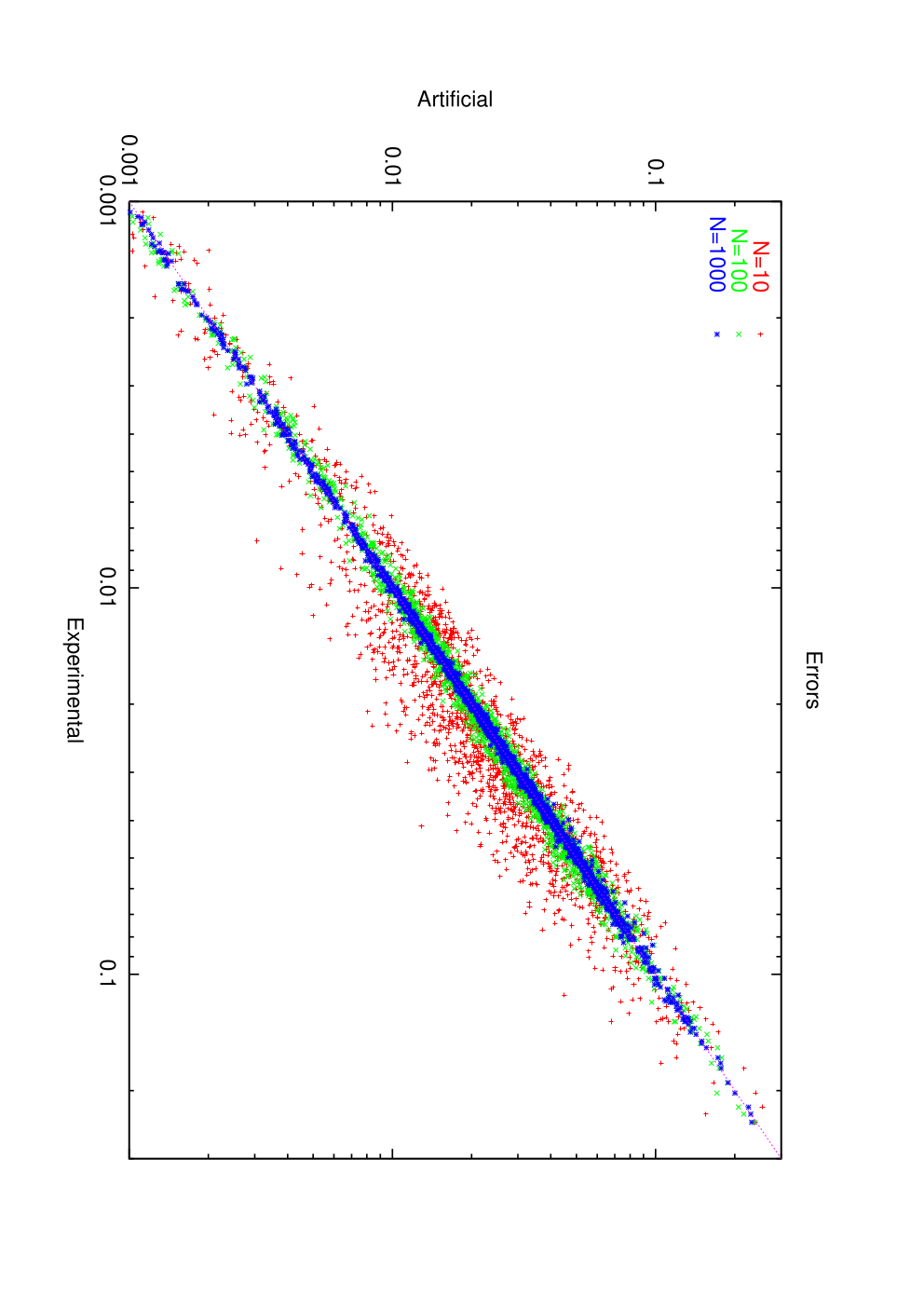
The value of is determined in such a way that the Monte Carlo set of replicas models faithfully the probability distribution of the data in the original set. A comparison of expectation values, variance and correlation of the Monte Carlo set with the corresponding input experimental values as a function of the number of replicas is shown in fig. 2, where we display scatter plots of the central values and errors for samples of 10, 100 and 1000 replicas. The corresponding plot for correlations is essentially the same as that shown in ref. [4]. A more quantitative comparison can be performed by defining suitable statistical estimators (see the appendix). Results are presented in table 2. Note in particular the scatter correlations for central values, errors and correlations, which indicate the size of the spread of data around a straight line. The table shows that a sample of 1000 replicas is sufficient to ensure average scatter correlations of 99% and accuracies of a few percent on structure functions, errors and correlations.
| 10 | 100 | 1000 | |
| 1.88% | 0.64% | 0.20% | |
| 0.99919 | 0.99992 | 0.99999 | |
| 37.21% | 11.77% | 3.43% | |
| 0.0292 | 0.0317 | 0.0316 | |
| 0.945 | 0.995 | 0.999 | |
| 0.3048 | 0.3115 | 0.2920 | |
| 0.696 | 0.951 | 0.995 | |
| 0.00013 | 0.00018 | 0.00015 | |
| 0.687 | 0.941 | 0.994 | |
neural networks [23] are then trained on the Monte Carlo data, by training each neural network on all the data points in the -th replica. The architecture of the networks is the same as in ref. [4]. The training is subdivided in three epochs, each based on the minimization of a different error function. In the first training epoch, the networks are trained to minimize the function
| (10) |
i.e., the deviation from the central value per data point. In the second epoch the function to be minimized is the uncorrelated per data point, namely, the computed omitting correlated systematics:
| (11) |
where is defined in eq. (3). Finally, in the third epoch the full per data point is minimized, namely
| (12) |
where is the covariance matrix for the -th replica, defined as in eq. (2), but with the normalization uncertainty included as an overall rescaling of the error due to the normalization offset of that replica: namely,
| (13) |
with
| (14) |
where is as in eq. (9). This is necessary in order to avoid a biased treatment of the normalization errors [22, 24].

The rationale behind this three-step procedure is that the true minimum which the fitting procedure must determine is that of the full eq. (12). However, this is nonlocal and time consuming to compute. It is therefore advantageous to look for its rough features at first, then refine its search, and finally determine its actual location.
The minimum during the first two epochs is found using back-propagation (BP) (see ref. [4]). This method is not suitable for the minimization of the nonlocal function eq. (12). In ref. [4] BP was used throughout, and the third epoch was omitted. This is acceptable provided the total systematics is small in comparison to the statistical errors, and indeed it was verified that a good approximation to the minimum of eq. (12) could be obtained from the ensemble of neural networks. This is no longer the case for the present extended data set, as we shall see explicitly in section 5. Therefore, the full eq. (12) is minimized in the third training epoch by means of genetic algorithms (GA), previously used and discussed by some of us for related purposes in ref. [25].
In comparison to previous work [4, 25], we have implemented several improvements, both in the BP and GA training epochs. In the BP epoch, we use on line training as in ref. [4], i.e. the parameters of the neural network are updated after each data point has been shown to it. This defines a training cycle. In ref. [4] it was shown that the length of training needed to achieve a given value of can differ significantly between experiments: it is larger for experiments which have smaller errors, contain more data, or cover kinematic regions where the structure function varies more rapidly. If one wants to end up with a similar value of for all experiments it is then necessary to adjust the relative length of training of different data sets. In ref. [4] this was achieved by finding by trial and error an optimal fixed weight for the two experiments included in the fit. This procedure is clearly not viable when the number of experiments is large. Therefore, we have implemented a dynamical weighted training, whereby the weight of each experiment is chosen initially to be the same for all experiments, and then adjusted dynamically according to the relative contribution of each experiment to the total eq. (12):
| (15) |
The value of is updated from the full data set every training cycles; because there are data points, this ensures that between updates each data point has been seen by the net about 700 times on average in the unweighted case. This method is not viable in the third (GA) training epoch, where can only be computed from the full set of data points (i.e., the training is necessarily batched, and not on-line). Therefore, one cannot choose to show a subset of data more often. One could in principle reweight the contribution of the single experiments to , but this might distort the global minimum in an unpredictable way.
In the GA epoch, we have introduced two improvements in comparison to the methods described in ref. [25]. First, we have introduced multiple mutations, specifically three nested mutations for each training cycle.11 1 Note that GA training cycles in ref. [25] are referred to as generations, as it is customary for genetic algorithms. The purpose of this is to avoid local minima, thereby increasing the speed of training. It is crucial that rates for these additional mutations are large, in order to allow for jumps from a local minimum to a deeper one. We find that one additional mutation with probability 20%, followed by two additional mutations with probability 4%, produce a significant improvement of the convergence rate. Second, we have introduced probabilistic selection. This entails that the sample of selected mutations is constructed by always selecting the mutation with the lowest value, plus mutations selected among the total mutations with probability
| (16) |
Namely, mutations with larger values are less likely to be selected but can still be selected with finite probability. This is helpful in allowing for mutations which only become beneficial after a combination of several individual mutations.
At the end of the GA training we are left with a sample of neural networks, from which e.g. the value of the structure function at can be computed as
| (17) |
The goodness of fit of the final set is thus measured by the per data point, which, given the large number of data points is essentially identical to the per degree of freedom:
| (18) |
where the average over replicas, denoted by , is defined in the appendix.
4 Training to the data
In order to apply the general method discussed in sect. 3 to the data presented in sect. 2 several specific issues must be addressed: the choice of training parameters and training length, the choice of the actual data set, and the choice of theoretical constraints. We now address these issues in turn.
The parameters and length for the first two training epochs have been determined by inspection of the fit of a neural network to the central experimental values. Clearly, this choice is less critical, in that it is only important in order for the training to be reasonably fast, but it does not impact on final result. We choose for the first BP epoch training cycles with learning rate and momentum term , and for the second BP epoch training cycles with learning rate and momentum term .
After these first two training epochs, the diagonal per data point eq. (11), which is being minimized, is of order two for the central data set. This is comparable to the length of training that was required to reach for the smaller data set of ref. [4]. The value of eq. (12), which is always bounded by it, is accordingly smaller (see table 3). The training algorithm then switches to GA minimization of the eq. (12). The determination of the length of this training epoch is critical, in that it controls the form of the final fit. This can only be done by looking at the features of the full Monte Carlo sample of neural networks.
| TABLE 3 | ||||
|---|---|---|---|---|
| A | B | |||
| Experiment | ||||
| Total | 2.05 | 1.54 | 2.03 | 1.36 |
| NMC | 1.97 | 1.56 | 1.74 | 1.54 |
| BCDMS | 1.93 | 1.66 | 1.32 | 1.26 |
| E665 | 1.64 | 1.37 | 1.83 | 1.38 |
| ZEUS94 | 3.15 | 2.26 | 3.01 | 2.21 |
| ZEUSBPC95 | 4.18 | 1.32 | 5.18 | 1.24 |
| ZEUSSVX95 | 3.37 | 1.88 | 5.68 | 2.11 |
| ZEUS97 | 2.33 | 1.54 | 3.02 | 1.37 |
| ZEUSBPT97 | 2.82 | 1.97 | 2.08 | 1.22 |
| H1SVX95 | 3.21 | 0.96 | 4.74 | 1.09 |
| H197 | 0.86 | 0.76 | 1.08 | 0.87 |
| H1LX97 | 1.96 | 1.46 | 1.50 | 1.18 |
| H199 | 1.15 | 1.07 | 1.10 | 1.01 |
| H100 | 1.59 | 1.50 | 1.48 | 1.26 |
Before addressing this issue, however, it turns out to be necessary to consider the possibility of introducing cuts in the data set. Indeed, consider the results obtained after a GA training of cycles (with mutation rate ) to the central data set, displayed in table 3. This is a rather long training: indeed, in each GA training cycle all the data are shown to the nets. Hence in GA cycles the data are shown to the nets times, comparable to the number of times they are shown to the nets during BP training. It is apparent that whereas for most experiments, it remains abnormally high for NMC and especially ZEUS94 and ZEUSSVX95. Because of the weighted training which has been adopted, this is unlikely to be due to insufficient training of these data sets, and is more likely related to problems of these data sets.
Whereas ZEUSSVX95 only contains a small number of data points, NMC and ZEUS94 account each for more than 10% of the total number of data points, and thus they can bias final results considerably. The case of NMC was discussed in detail in ref. [4]. This data set is the only one to cover the medium-, medium-small region (compare figure 1) and thus it cannot be excluded from the fit. As discussed in ref. [4], the relatively large value of for this experiment is a consequence of internal inconsistencies within the data set. A value of indicates that the neural nets do not reproduce the subset of data which are incompatible with the bulk, as it should be, whereas a value could only be obtained by overlearning, i.e. essentially by fitting irrelevant fluctuations (see ref. [4]).
Let us now consider the case of ZEUS94. The kinematic region of this experiment is entirely covered by ZEUS97, H197, H199, H100. We can therefore study the impact of excluding this experiment from the global fit, without information loss. The results obtained in such case are displayed in table 4: when the experiment is not fitted the value for all experiments with which it overlaps improves and so does the global , whereas for ZEUS94 itself only deteriorates by a comparable amount, despite the fact that the experiment is now not fitted at all. We conclude that the experiment should be excluded from the fit, since its inclusion result in a deterioration of the fit quality, whereas its exclusion does not entail information loss. Difficulties in the inclusion of this experiment in global fits were already pointed out in refs. [26, 27], where it was suggested that they may be due to underestimated or nongaussian uncertainties. It is likely that ZEUSSVX95 has similar problems. However, its inclusion in the fit is no reason of concern, even if its high value were due to incompatibility of this experiment with the others or underestimate of its experimental uncertainties, because of the small number of data points. It is therefore retained in the data set. Our final data set thus includes all experiments in table 1, except ZEUS94. We are thus left with 1698 data points.
| TABLE 4 | |
|---|---|
| Experiment | |
| Total | 1.25 |
| NMC | 1.51 |
| BCDMS | 1.24 |
| E665 | 1.23 |
| ZEUS94 | 2.28 |
| ZEUSBPC95 | 1.16 |
| ZEUSSVX95 | 2.08 |
| ZEUS97 | 1.37 |
| ZEUSBPT97 | 1.00 |
| H1SVX95 | 1.04 |
| H197 | 0.84 |
| H1LX97 | 1.19 |
| H199 | 1.00 |
| H100 | 1.24 |
For the sake of future applications, it is interesting to ask how the procedure of selecting experiments in the data set can be automatized. This can be done in an iterative way as follows: first, a neural net (or sample of neural nets) is trained on only one experiment; then, the total for the full data set is computed using this neural net (or sample of nets); the procedure is then repeated for all experiments, and the experiment which leads to the smallest total is selected. In the second iteration, the net (or sample of nets) is trained on the experiment selected in the first iteration plus any of the other experiments, thereby leading to the selection of a second experiment to be added to that selected previously, and so on. The process can be terminated before all experiments are selected, for instance if it is seen that the addition of a new experiment does not lead to a significant improvement in for given length of training.


We now proceed to discuss the length of training for our final data set. The eq. (18) is shown in figure 3 as a function of the number of GA training cycles. The decreases very rapidly during the first few hundreds of training cycles. After about 5000 training cycles, the as a function of the training length essentially flattens for all experiments but BCDMS. The further decrease of the total is then due essentially to the decrease of the contribution from BCDMS. A training length of GA cycles is necessary in order for the of BCDMS to flatten out at . As discussed in ref. [4], the BCDMS data can only be learnt with a longer training because they have high precision while being located in the intermediate (valence) region, where the parton distribution displays significant variation.
The values for the fit of a neural net to the central data with this training is given in table 3. It shows that all experiments are well reproduced with the exceptions discussed above. It is interesting to observe that while eq. (12) decreases significantly during the GA training, the uncorrelated eq. (11) decreases marginally, and in fact it actually increases for several HERA experiments. This shows that correlations are sizable for the HERA experiments, so that the approach of ref. [4], based on the minimization of eq. (11), is not adequate in this case. GA minimization appears to be very efficient in reducing the value relatively fast.
We finally turn to the issue of theoretical constraints. The only theoretical assumption on the shape of is that it satisfies the kinematic constraint for all . As this constraint is local, its implementation is straightforward: it can be enforced by including in the data set a number of artificial data points which satisfy the constraint with a suitably tuned error. In the present fit we have checked that the best choice is to add a number of artificial points at , equal to 2% of the experimental trained points (33 points with ZEUS94 excluded from the fits), and with error equal to one tenth of the mean statistical error of the trained points. These points are equally spaced in , within the range covered by the trained points.
5 Results
The result of the minimization of a single neural net to the central data points is shown in table 4. The results for the final set of 1000 neural networks are displayed in table 5, while in table 6 we give the details of results for each experiment. Note that the figure of merit for the minimization eq. (12) and its average defined in the appendix eq. (30) differs from the full eq. (18) not only because the latter is computed from the structure function averaged over nets eq. (17), but also because of the different treatment of normalization errors in the respective covariance matrices eq. (13) and eq. (2).
Besides the we also list the values of various quantities, defined in the appendix, which can be used to assess the goodness of fit.
| 1000 | |
| 1.18 | |
| 2.52 | |
| 0.99 | |
| 0.54 | |
| 0.027 | |
| 0.008 | |
| 0.73 | |
| 0.20 | |
| 0.31 | |
| 0.67 | |
| 0.54 | |
| 0.49 | |
| Experiment | NMC | BCDMS | E665 |
|---|---|---|---|
| 1.47 | 1.19 | 1.20 | |
| 2.69 | 3.17 | 2.29 | |
| 0.96 | 0.99 | 0.91 | |
| 0.59 | 0.50 | 0.56 | |
| 0.0013 | |||
| 0.63 | 0.56 | 0.89 | |
| 0.017 | 0.007 | 0.032 | |
| 0.008 | 0.005 | 0.008 | |
| 0.23 | 0.98 | 0.17 | |
| 0.51 | 0.69 | 0.29 | |
| 0.17 | 0.52 | 0.20 | |
| 0.84 | 0.86 | 0.60 | |
| 0.08 | 0.73 | 0.05 | |
| -0.03 | 0.98 | 0.16 |
| Experiment | ZEUSBPC95 | ZEUSSVX95 | ZEUS97 | ZEUSBPT97 | H1SVX95 | H197 | H1LX97 | H199 | H100 |
|---|---|---|---|---|---|---|---|---|---|
| 1.02 | 2.08 | 1.35 | 0.86 | 0.67 | 0.71 | 1.07 | 0.90 | 1.11 | |
| 2.07 | 2.03 | 2.24 | 2.08 | 2.03 | 1.91 | 2.41 | 1.93 | 2.11 | |
| 0.98 | 0.96 | 0.99 | 0.99 | 0.97 | 0.99 | 0.99 | 0.98 | 0.99 | |
| 0.51 | 0.66 | 0.55 | 0.55 | 0.44 | 0.46 | 0.53 | 0.48 | 0.54 | |
| 0.0035 | 0.0010 | 0.0043 | 0.0030 | 0.0005 | 0.003 | 0.0013 | |||
| 0.91 | 0.94 | 0.87 | 0.72 | 0.96 | 0.95 | 0.75 | 0.96 | 0.93 | |
| 0.022 | 0.061 | 0.037 | 0.012 | 0.063 | 0.040 | 0.027 | 0.051 | 0.030 | |
| 0.006 | 0.013 | 0.011 | 0.006 | 0.011 | 0.008 | 0.008 | 0.008 | 0.009 | |
| 0.85 | 0.72 | 0.86 | 0.73 | 0.84 | 0.87 | 0.42 | 0.82 | 0.89 | |
| 0.09 | 0.30 | 0.12 | 0.14 | 0.118 | 0.14 | 0.31 | 0.16 | 0.14 | |
| 0.61 | 0.24 | 0.28 | 0.40 | 0.36 | 0.06 | 0.29 | 0.05 | 0.09 | |
| 0.77 | 0.64 | 0.39 | 0.63 | 0.57 | 0.27 | 0.58 | 0.29 | 0.26 | |
| 0.53 | 0.40 | 0.66 | 0.60 | 0.48 | 0.51 | 0.69 | 0.37 | 0.55 | |
| 0.0014 | |||||||||
| 0.69 | 0.48 | 0.77 | 0.65 | 0.53 | 0.61 | 0.57 | 0.54 | 0.58 |
The quality of the final fit is somewhat better than that of the fit to the central data points shown in table 4. In particular, with the exception of NMC (which is likely to have internal inconsistencies [4]) and ZEUSSVX95 (which is likely to have the same problems as those of ZEUS94 discussed in section 4) the per degree of freedom is of order 1 for all experiments. It is interesting to note that the for the neural network average is rather better than the average eq. (30). The (scatter) correlation between experimental data and the neural network prediction equals one to about 1% accuracy, with the exception of NMC, ZEUSSVX95 (which have the aforementioned problems) and E665. The E665 kinematic region overlaps almost entirely (apart from very small GeV2) with that of NMC and BCDMS, while having lower accuracy (this is why the experiment was not included in the fits of ref. [4]). The data points corresponding to this experiment are therefore essentially predicted by the fit to other experiments, thus explaining the somewhat smaller scatter correlation.
The average neural network variance is in general substantially smaller than the average experimental error, typically by a factor . This is the reason why : the neural nets fluctuate less about central experimental values than the Monte Carlo replicas. In the presence of substantial error reduction, the (scatter) correlation between network covariance and experimental error is generally not very high, and can take low values when a small number of data points from one experiment is enough to determine the outcome of the fit, such as in the case of the NMC experiment, even more so for E665. [4]

As discussed extensively in ref. [4] it is important to make sure that this is due to the fact that information from individual data points is combined through an underlying law by the neural networks, and not due to parametrization bias. To this purpose, the -estimator has been introduced in ref. [4], where it was shown that in the presence of substantial error reduction if there is parametrization bias, whereas in the absence of parametrization bias.22 2 Note that in ref. [4] the -ratio was defined in terms of the diagonal eq. (11), because neural networks were trained by minimizing that quantity. It is easy to see that the results of ref. [4] for remain true when the full eq. (12) is minimized, provided is redefined accordingly. It is apparent from tables 5-6 that indeed for all experiments. Note that, contrary to what was found in ref. [4], there is now some error reduction also for the BCDMS experiment, though by a somewhat smaller amount than for other experiments. We will come back to this issue when comparing results to those of ref. [4].
Further evidence that the error reduction is not due to parametrization bias can be obtained by studying the dependence of on the length of training. This dependence is shown in fig. 4 for the BCDMS experiment. It is apparent that the error reduction is correlated with the goodness of fit displayed in fig. 3, and it occurs during the GA training, thereby suggesting that error reduction occurs when the neural networks start reproducing an underlying law. If error reduction were due to parametrization bias it would be essentially independent of the length of training.

The point-to-point correlation of the neural nets is somewhat larger than that of the data, as one might expect as a consequence of an underlying law which is being learnt by the neural nets. In fact, for the NMC experiment the increase in correlation essentially compensates the reduction in error, in such a way that the average covariance of the nets and the data are essentially the same. This again shows that in the case of the NMC experiment a small number of points is sufficient to predict the remaining ones. For all other experiments, however, the covariance of the nets is substantially smaller than that of the data. As a consequence the (scatter) correlation of covariance remains relatively high for all experiments, except NMC, and especially E665 whose points are essentially predicted by the fit to other experiments.


The structure function and associated one- error band is compared to the data as a function of for a pair of typical values of in fig. 5. In fig. 6 the behaviour of the structure function as a function of at fixed and as a function of at fixed is also shown. It is apparent that in the data region the error on the neural nets is rather smaller than that on the data used to train them. The error however grows rapidly as soon as the nets are extrapolated outside the region of the data. At large , however, the extrapolation is kept under control by the kinematic constraint .


Let us finally compare the determination of presented here with that of ref. [4], which was based on pre-HERA data. In fig. 7 one- error bands for the two parametrizations are compared, whereas in fig. 8 we display the relative pull of the two parametrizations, defined as
| (19) |
where is the error on the structure function determined as the variance of the neural network sample. In view of the fact that the old fit only included BCDMS and NMC data, it is interesting to consider four regions: (a) the BCDMS region (large , intermediate , e.g. , GeV2); (b) the NMC region (intermediate , not too large , e.g. , GeV2); (c) the HERA region (small and large , e.g. and GeV2); (d) the region where neither the old nor the new fit had data (very large or very small ). In region (a) the new fit is rather more precise than the old one, for reasons to be discussed shortly, while central values agree, with ). In region (b) the new fit is significantly more precise than the old one, while central values agree to about one sigma. In region (c) the new fit is rather accurate while the old fit had large errors, but nevertheless, because the HERA rise of is outside the error bands extrapolated from NMC. This shows that even though errors on extrapolated data grow rapidly they become unreliable when extrapolating far from the data. Finally in region (d) all errors are very large and is consequently small, except at small and large , where the new fits extrapolate the rise in the HERA data, which is missing altogether in the old fits.

Let us finally come to the issue of the BCDMS error, which, as already mentioned, is reduced somewhat in the current fit in comparison to the data and the previous fit. This may appear surprizing, in that the new fit does not contain any new data in the BCDMS region. However, as is apparent from fig. 4, this error reduction takes place in the GA training stage, when eq. (12) is minimized. Furthermore, we have verified that if the uncorrelated eq. (11) is minimized during the GA training no error reduction is observed for BCDMS. Hence, we conclude that the reason why error reduction for BCDMS was not found in ref. [4] is that in that reference neural networks were trained by minimizing . In fact, as discussed in sect. 4, the BCDMS experiment turns out to require the longest time to learn, especially after inclusion of the HERA data. Error reduction only obtains after this lenghty minimization process.
6 Conclusion
We have presented a determination of the probability density in the space of structure functions for the structure function for the proton, based on all available data from the NMC, BCDMS, E665, ZEUS and H1 collaborations. Our results take the form of a Monte Carlo sample of 1000 neural networks, each of which provides a determination of the structure function for all . The structure function and its statistical moments (errors, correlations and so on) can be determined by averaging over this sample. Results are made available as a FORTRAN routine which gives , determined by a set of parameters, and 1000 sets of parameters corresponding to the Monte Carlo sample of structure functions. They can be downloaded from the web site http://sophia.ecm.ub.es/f2neural/.
This works updates and upgrades that of ref. [4], where similar results were obtained from the BCDMS and NMC data only. The main improvements in the present work are related to the need of handling a large number of experimental data, affected by large correlated systematics. Apart from many smaller technical aspects, the main improvement introduced here is the use of genetic algorithms to train neural networks on top of back-propagation. This has allowed for a more accurate handling of correlated systematics.
Whereas the results of this paper may be of direct practical use for any application where an accurate determination of and its associate error are necessary, its main motivation is the development of a set of techniques which will be required for the construction of a full set of parton distributions with faithful uncertainty estimation based on the same method. This will be presented in a forthcoming publication.
Acknowledgments
We thank M. Arneodo, E. Rizvi, E. Tassi and F. Zomer for informations on the HERA data, and G. d’Agostini, L. Garrido and G. Ridolfi for discussions. This work has been supported by the project GC2001SGR-00065 and by the Spanish grant AP2002-2415.
Appendix A Statistical estimators
We define various statistical estimators which have been used in the paper. The superscripts , and refer respectively to the original data, to the Monte Carlo replicas of the data, and to the neural networks. The subscripts and refer respectively to whether averages are taken by summing over all replicas or over all data.
- •
Replica averages
- –
Average over the number of replicas for each experimental point
(20) - –
Associated variance
(21) - –
Associated covariance
(22) (23) - –
Mean variance and percentage error on central values over the data points.
(24) (25) We define analogously , , and .
- –
- –
Average variance:
(29) We define analogously and , as well as the corresponding experimental quantities.
- –
- •
Neural network averages
- –
- –
Mean variance and percentage error on central values over the data points.
(31) (32) - –
We define analogously percentage errors on the correlation and covariance.
- –
Scatter correlation
(33) We define analogously and .
- –
References
- [1] See e.g. W. K. Tung, hep-ph/0409145 and refs. therein.
- [2] S. Forte, J. I. Latorre, L. Magnea and A. Piccione, Nucl. Phys. B 643 (2002) 477.
- [3] B. Adeva et al. [Spin Muon Collaboration], Phys. Rev. D 58 (1998) 112002.
- [4] S. Forte, L. Garrido, J.I. Latorre, A. Piccione, JHEP 0205 (2002) 062, hep-ph/0204232.
- [5] See e.g. the HEPDATA database, http://durpdg.dur.ac.uk/HEPDATA/.
- [6] M. Arneodo et al. [New Muon Collaboration], Nucl. Phys. B 483 (1997) 3.
- [7] A. C. Benvenuti et al. [BCDMS Collaboration], Phys. Lett. B 223 (1989) 485.
- [8] M. R. Adams et al. [E665 Collaboration], Phys. Rev. D 54 (1996) 3006.
- [9] M. Derrick et al. [ZEUS Collaboration], Z. Phys. C 72 (1996) 399.
- [10] J. Breitweg et al. [ZEUS Collaboration], Phys. Lett. B 407 (1997) 432.
- [11] J. Breitweg et al. [ZEUS Collaboration], Eur. Phys. J. C 7 (1999) 609.
- [12] S. Chekanov et al. [ZEUS Collaboration], Eur. Phys. J. C 21 (2001) 443.
- [13] J. Breitweg et al. [ZEUS Collaboration], Phys. Lett. B 487 (2000) 53.
- [14] C. Adloff et al. [H1 Collaboration], Nucl. Phys. B 497 (1997) 3.
- [15] C. Adloff et al. [H1 Collaboration], Eur. Phys. J. C 13 (2000) 609.
- [16] C. Adloff et al. [H1 Collaboration], Eur. Phys. J. C 21 (2001) 33.
- [17] C. Adloff et al. [H1 Collaboration], Eur. Phys. J. C 19 (2001) 269.
- [18] C. Adloff et al. [H1 Collaboration], Eur. Phys. J. C 30 (2003) 1.
- [19] S. Eidelman et al. [Particle Data Group Collaboration], Phys. Lett. B 592 (2004) 1.
- [20]
R. Barlow,
eConf C030908 (2003) WEMT002, physics/0401042;
physics/0306138. - [21] G. D’Agostini, physics/0403086.
- [22] “Bayesian reasoning in data analysis: A critical introduction” (World Scientific, Singapore, 2003).
- [23]
C. Peterson and T. Rognvaldsson,
Lectures at the 1991 CERN School of Computing, preprint
LU-TP-91-23;
B. Müller, J. Reinhardt and M. T. Strickland, Neural Networks: an introduction (Springer, Berlin, 1995);
G. Stimpfl-Abele and L. Garrido, Comput. Phys. Commun. 64 (1991) 46. - [24] G. D’Agostini, Nucl. Instrum. Meth. A 346 (1994) 306.
- [25] J. Rojo and J. I. Latorre, JHEP 0401, 055 (2004).
- [26] W. T. Giele, S. A. Keller and D. A. Kosower, hep-ph/0104052.
- [27] S. I. Alekhin, Phys. Rev. D 63 (2001) 094022.