Diffractive Vector Meson Production at HERA:
from Soft to Hard QCD Thanks: To be published in Physics of Elementary
Particles and Atomic Nucleai, JINR, Russia
Abstract
Experimental results from HERA on diffractive vector meson production and their theoretical interpretation within microscopic QCD are reviewed with an emphasis on the BFKL color dipole and -factorization approaches.
DESY–04–243
1 Introduction
1.1 The motivation
The Deep Inelastic Scattering (DIS) of leptons off hadrons is interpreted as a knockout of one of the charged partons of the target by hard Rutherford scattering followed by a complete shattering of the target nucleon or nucleus. One of major discoveries at the electron-proton collider HERA at DESY was the observation that the large rapidity gap events, in which the target nucleon emerges in the final state with a loss of a very small fraction of its energy-momentum, constitute a substantial and approximately scaling fraction of high-energy/small- DIS of electrons and positrons on protons [1, 2]. Although the major features of such events and their cross sections have been correctly predicted within perturbative QCD [3], the very existence of large rapidity gap events for nuclear targets is nearly paradoxical: as well known the deposition of dozen MeV energy is already sufficient to break up the target nucleus, still the theory predicts that for a sufficiently heavy nucleus and for the Bjorken variable the fraction of rapidity-gap DIS with retention of the target nucleus in exactly the ground state must be exactly 50 per cent [4] and there is a direct evidence for that from the E665 Fermilab experiment [5]. The discovery of rapidity gaps at HERA has led to a renaissance of the physics of diffractive scattering in an entirely new domain, in which the large momentum transfer from leptons provides a hard scale. It also vindicated the early suggestions of Bjorken to look for hard diffraction in hadronic interactions [6] and stimulated a revival of the rapidity gap physics with hard triggers — large- jets, -bosons, excitation of heavy flavors, — at the proton-antiproton collider Tevatron (for the recent review see [7, 8, 9] and references therein). Whether the existence of such a hard scale makes the diffractive DIS tractable within the perturbative QCD or not has been a subject of intense theoretical and experimental research during the past decade or so. A good summary of the pre-1997 status of the vector meson production physics is found in the monograph of Crittenden [10], the pre-1999 status of theoretical ideas on diffractive DIS was reviewed by Hebecker [11]), for the general introduction into the physics of diffractive scattering see the recent books of Barone and Predazzi [12] and Forshaw and Ross [13].
The subject of this review is a special case of diffractive DIS — the exclusive production of vector mesons. One disclaimer is in order: we focus on the high-energy and/or very small- regime dominated by the pQCD pomeron exchange and, facing the size limitations, don’t discuss very interesting low to moderate energy data from the HERMES collaboration which are strongly affected by the non-vacuum exchanges (for the review and references see [14]). The past decade the topic of high-energy diffraction has been dominated by new fundamental data coming from the ZEUS and H1 experiments at HERA. The interest in the exclusive electroproduction of vector mesons is multifold. From the purely experimental point of view, the HERA experiments offer a prime example of diffractive scattering at energies much higher than were attainable before. Furthermore, the self-analyzing decays of spin-1 vector mesons allow one to unravel the mechanism of diffraction in full complexity. Specifically, the HERA experiments for the first time gave an unequivocal proof that the -channel helicity non-conservation persists at highest available energies [15, 16]. On the theoretical side, starting from the seminal papers on the color dipole approach by Kopeliovich, Zakharov et al. [17, 18, 19, 20, 21] and the related momentum space approach by Ryskin [22] and Brodsky et al. [23], it has been understood that the exclusive diffractive production of vector mesons in DIS is a genuinely hard phenomenon, whose major features can be described by pQCD. This can be understood in terms of the shrinkage of the photon with the increase of the hard scale [24, 17, 18], and because of this shrinkage the diffractive production probes the hadronic properties of the photon and vector mesons at short distances. One of the direct manifestations of this shrinkage of the photon is a decrease of the diffraction slope with the increase of the hard scale [25, 26, *NNPZZslopeVM1], which has for the first time been observed at HERA [28, 29], for the earlier evidence from the NMC experiment see [30]. Finally, the presence of the hard scale enables one to test the modern theoretical ideas on the mechanism of the -channel exchange with vacuum quantum numbers, i.e., the QCD Pomeron. The way the QCD Pomeron is probed in diffractive vector meson production is similar to, but still different from, that in the conventional inclusive DIS. For instance, large- diffractive production of vector mesons probes the QCD Pomeron in a hard regime [31] inaccessible in inclusive DIS.
1.2 From inclusive DIS to DVCS to exclusive vector meson production
To this end recall the basics of inclusive DIS of leptons off nucleons
To the lowest order in QED it is treated in the one-photon exchange approximation. The leptons serve as a source of virtual photons of energy and virtuality (the scattering kinematics and the 4-momenta are shown in Fig. 1) and the fundamental process is the virtual photoabsorption
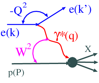
In the fully inclusive DIS only the scattered lepton is detected and one sums over all the hadronic final states . Then the observed inclusive DIS cross section is proportional to the absorptive part of the forward, at vanishing momentum transfer , virtual Compton scattering amplitude shown in Fig. 2

| (1) |
and, invoking the optical theorem, can be cast in the form of the flux of virtual transverse and scalar (longitudinal) photons times the total photoabsorption cross sections and .
Now take a closer look at the Compton scattering amplitude as a function of the virtuality of the incident and final state photons, and , respectively. In fully inclusive DIS this amplitude is accessible only for and at vanishing momentum transfer . When continued analytically to the amplitude will describe the exclusive real photon production often referred to as the Deeply Virtual Compton Scattering (DVCS) [32]
| (2) |
while the further continuation to gives the amplitude of the exclusive vector meson production
| (3) |
Both DVCS and exclusive vector meson production can be studied experimentally by selecting a special final state or , respectively. Furthermore, both reactions can be studied at the non-vanishing momentum transfer , i.e., , for the definition of the kinematical variables see Fig. 3.

The point that inclusive DIS, DVCS, and exclusive vector meson production are described by the same analytic function taken at different values of suggests from the very outset the complementary probe of high energy pQCD in the three reactions (1), (2), and (3). For instance, in the forward, , Compton scattering probed in inclusive DIS the helicity flip amplitudes vanish for the kinematical reason. In contrast to that, the inclusive vector meson production at enables one to determine the full set of helicity-conserving and helicity-flip amplitudes and investigate the spin properties of hard (generalized) Compton scattering to full complexity.
1.3 When vector meson production is dominated by small color dipole interactions?
The intimate relationship between inclusive DIS, DVCS, and exclusive vector meson production is still better seen in the lightcone color dipole picture of small- DIS which illustrates nicely the interplay of the scattering mechanism and the (partonic) structure of particles. It is needless to recall the outstanding role of the photon-matter interactions in the conception and formation of the quantum mechanics and quantum field theory. In the early years of the nonrelativistic quantum mechanics the photon has been regarded as structureless and the focus of the theory was on spectral lines, photo-effect and the related phenomena. With the advent of the first quantum field theory — the Quantum Electro Dynamics (QED), — it has become clear that the fundamental transition
| (4) |
between bare particles gives rise to a concept of a dressed physical photon that contains all bare states to which it couples via (4) and still higher order QED processes. At low energies, the virtual vacuum polarization gives rise to the well known Uehling-Serber radiative correction to the Coulomb potential; at higher energies the familiar Bethe-Heitler pair production in the Coulomb field of a nucleus can be viewed as materialization of the component of the physical photon (see Bjorken, Kogut, Soper [33]). The Compton scattering which is behind inclusive DIS at very small values of the Bjorken variable can be viewed as (i) the transition of the virtual photon to the pair (the color dipole) at a large distance
| (5) |
upstream the target (here is the nucleon mass), (ii) interaction of the color dipole with the target nucleon, and (iii) the projection of the scattered onto the virtual photon (Fig. 4a). Notice the very special choice of the stage (iii): if one lets the scattered color dipole materialize as hadrons, one ends up with the large rapidity gap DIS — the diffractive excitation . Here the production of continuum hadronic states is modeled by the continuum states (Fig. 4b), whereas the projection of the scattered color dipole onto the vector meson gives the exclusive (diffractive, elastic) vector meson production, and projection onto the real photon gives so-called DVCS (Fig. 4c).

The amplitude of the transition of the photon into the state, alias the wave function of the photon, and the amplitude of scattering the color dipole off the target are the universal ingredients in all the processes. The wave function of the virtual photon is well known [24], and different processes probe the color dipole scattering amplitude at different dipole sizes [18].
For instance, irrespective of the photon’s virtuality , the inclusive diffractive DIS into the continuum states is controlled for the most part by interaction of large color dipoles [3]. The scaling violations in the proton structure function (SF), , come from small color dipoles of size
| (6) |
whereas the absolute value of receives contributions from large to small dipole sizes [34, 35],
| (7) |
In contrast to the inclusive DIS and inclusive diffractive DIS, the amplitude of the exclusive vector meson production is dominated by the contribution from small dipoles of size [18, 19]
| (8) |
often referred to as the scanning radius (formula (8) is applicable only if is smaller than the typical hadron size). This, exclusive vector meson production offers a cleaner environment for testing transition from soft to hard scattering.
The color dipole formalism is entirely equivalent to the BFKL formalism of the (transverse) momentum dependent gluon distributions in the leading approximation [36, 37, *KLF771, 39]. Within this formalism, often referred to as the -factorization, Eq. (8) suggests that the vector meson production probes the gluon density of the target at pQCD hard scale [22, 19, 20, 21, 40]
| (9) |
which is large for heavy quarkonia () or for large . In the hard regime of small scanning radius, the vector meson production amplitudes will only depend on the wave function of vector mesons at a vanishing quark-antiquark separation in the two-dimensional transverse, or impact-parameter, space. There still remains a certain sensitivity to the separation of quarks in the longitudinal direction, which nonrelativistically is conjugate to the longitudinal Fermi motion of the quark and antiquark in the vector meson or the partition of the longitudinal momentum of the vector meson between the quark and antiquark in the relativistic lightcone language. As a result, the vector meson production amplitude is not calculable from the first principles of pQCD, still the sensitivity to the soft input can to a large extent be constrained by the decay , which proceeds via the short-distance annihilation . Then Eq. (8) suggests that, upon factoring out the emerging decay amplitude, the vector meson production amplitudes will depend on the hard scale in a universal manner. Finally, the energy dependence of the vector meson production amplitude offers a more local probe of the properties of the hard pQCD Pomeron than the inclusive DIS.
1.4 The scale for the onset of hard regime
Before opening the issue of hard production of vector mesons, one needs to define the typical soft production. Here a brief comment on the venerable Vector Dominance Model (VDM) is in order. Because of the obvious dominance by the vector meson pole contribution, the point that at the amplitude of the production of the timelike virtual photon will be proportional to the appropriate vector meson production amplitude times the transition amplitude is a tautology. Experimentally, the timelike photons are produced in the annihilation and the transition amplitudes are measured at the colliders and, of course, in the decay . The assumption that the ground state vector meson pole contribution dominates the photoproduction amplitudes, and the transition amplitude does not vary substantially from the vector meson pole down to is the basis of the very successful VDM as formulated by Sakurai [41], Gell-Mann, Zachariasen, Scharp and Wagner [42, 43] (for the comprehensive review of foundations and tests of the VDM, see Bauer et al. [44, *BauerRevModPhys1]).
From the color dipole point of view, the success of the VDM in real photoproduction derives from the proximity of the distribution of color dipoles in the ground state vector mesons and in the real photon. So, the component of the physical photon can be approximated by the corresponding vector meson (quarkonium) and the amplitude of interaction of the color dipole with the nucleon can be approximated by the vector meson-nucleon scattering amplitude, for an illustration see Fig. 5.

From the naive quark model viewpoint, the -meson is the hyperfine partner of the -meson and the 2-dimensional charge radius, , of the sets the relevant scale.
One comes to the same conclusion from the experimentall observation that to a very good accuracy the -dependence of elastic scattering, real Compton scattering and real photoptoduction is the same [44, *BauerRevModPhys1, 46]. Indeed, within the VDM which is a very good approximation for real photons, the differential cross sections of the latter two processes are proportional to the differential cross section of elastic sacttering. Then the equal -dependence of the and elastic scattering entails an equality of t he radii of he -meson.
Experimentally, the charge form factor of the pion is well described by the VDM -pole formula and [47, 48]
| (10) |
The onset of the hard regime in diffractive vector meson production requires that the scanning radius is smaller than any other hadronic scale. First place, one needs , i.e.,
| (11) |
The corrections in the small parameter depend on the wave function (WF) of the vector meson. With the soft, Gaussian, wave function, , in order for the WF-dependent corrections not to exceed one needs . For the hard, Coulomb-like, wave functions, , a still higher is needed for a similar insensitivity to the shape of the wave function, for the related discussion of the onset of pQCD see [49]. Even for the heavy the scanning radius at is large,
| (12) |
(for the charmonium parameters see [50, 51, 52]), so that for the onset of the short-distance regime insensitive to the shape of the wave function of the one needs . In the realistic QCD there is still another scale - the propagation radius for perturbative gluons which is small, fm (for the lattice QCD evaluations of see [53], for the origin of in the instanton models of QCD vacuum see [54], the analysis of heavy quarkonia decays is found in [55]). The color dipole cross section is of true pQCD origin only for dipoles , i.e., the fully pQCD description of diffractive vector mesons requires , i.e.,
| (13) |
One must not be discouraged, though: the -dependence of the dipole cross section does not change any dramatically from the pure pQCD domain of to the non-perturbative domain of , and the fundamental concept of the scanning radius remains viable up to fm, see also the discussion in Sect. 3.3.2.
The large momentum transfer, , is still another way to probe the structure of the photon and vector meson at short distances, . It is generally believed [56, 49] that supersedes as a hard scale if . The caveats of as large scale and of single BFKL pomeron exchange dominance will will be discussed to more detail in Sect. 4.11.
1.5 The structure of the review
In this review we focus on the onset of hard pQCD regime in exclusive vector meson production at HERA. The presentation of the experimental data and of theoretical ideas goes in parallel, and an intimate connection between the vector meson production and the inclusive DIS will be repeatedly underlined. For this reason the presentation of the theoretical ideas on vector meson production will be heavily biased towards the color dipole picture and its momentum-space counterpart — the so-called -factorization.
The brief description of the H1 and ZEUS detectors, the kinematics of DIS and of the vector meson production, the event selection, the definition of major observables and of the spin density matrix of virtual photons is presented in Section 2. The subject of Section 3 is an overview of basic theoretical ideas on the vector meson production. Here we discuss briefly the Regge theory of the soft photon and hadron interactions, the QCD approach to the vacuum exchange (the Pomeron), the flavor dependence, the connection between the vector meson production and the leptonic decay of vector mesons, the origin of -channel helicity non-conservation (SCHNC) and the exclusive-inclusive duality connection between inclusive diffractive DIS and vector meson production. We also introduce the color dipole approach to DIS and vector meson production and explain how the shrinkage of virtual photons makes the vector meson production pQCD tractable. The unified microscopic QCD approach to small- DIS and diffractive vector meson production — the -factorization approach, which is equivalent to the color dipole approach, — is presented to more detail in Section 4. Here we discuss both the small- production within the diffraction cone and major ideas on large- proton dissociative reaction. This section can be skipped in the first reading, but is essential for understanding the status of theoretical calculations of the vector meson production.
In Section 5 we start the presentation of the physics results with the helicity structure of the vector meson production. This includes the definition of the spin observables, an introduction into the important subject of the s-channel helicity non-conservation (SCHNC) and the comparison of the experimental data on the spin density matrix of produced vector mesons with the theoretical expectations from the color-dipole/-factorization approach 11 1 Throughout this review, the numerical results shown for the -factorization are either taken from the PhD thesis [57] or performed specially for this review [58]. In Section 6 we discuss the -dependence of the vector meson production cross sections as well as the longitudinal-to-transverse cross sections ratios . We put special emphasis on the flavor dependence of cross sections, emphasize an importance of as the hard pQCD scale and comment on the sensitivity of to the short distance wave function of vector mesons. In Section 7 we review the experimental data on the energy dependence of the cross sections and its theoretical interpretation in terms of the Pomeron exchange. We show how the the change of the energy dependence from light to heavy flavors and from photoproduction to DIS is controlled by as the hard pQCD scale. We comment on tricky points in comparison of hard scales and energy dependence in inclusive DIS and diffractive vector meson production and on the impact of interplay of the scanning radius and the position of the node of the radial wave function for the production cross section. The focus of Section 8 is on the -dependence of the cross sections, both in the low- and high- regimes. The discussion of low- data centers on the , and -dependence of the slope of diffraction cone. The recurrent theme is a universality of diffraction slopes as a function of the scanning radius and/or as the hard pQCD scale. The properties of the Pomeron trajectory extracted from the vector meson production data are discussed in detail: the experimentally observed shrinkage of the diffraction cone for the production gives a strong evidence for which decreases with approximately linearly at , but then starts rising up to in the hard regime of large . Finally, in Section 9, we summarize the principal findings from HERA experiments on diffractive vector meson production and list open issues in the pQCD interpretation of these data.
It is important to mention here that not all currently available HERA data are always shown in each plot where they may belong to. This is because sometimes the published plots from H1, ZEUS and other authors are used without any modifications. This is especially valid for the ”preliminary” H1 and ZEUS plots, that have been shown to the conferences and are not yet submitted in form of ”official” papers. Such plots are just taken as they are. If for some compilation and figures only very recent data are used it is explained in the correspondent caption.
2 The experimental overview
2.1 HERA
HERA(Hadron Electron Ring Anlage) is the world’s first lepton-proton collider located at Deutsches Elektronen Synchrotron (DESY) site in Hamburg, Germany (see e.g. [59] and references therein). The HERA ring has a circumference of about 6.3 km with two separated synchrotron rings for electrons (positrons) and protons. It runs 10-30 m below ground level and has four experimental areas. In two of them the beams are made to collide to provide interactions for the experiments H1 and ZEUS. The remaining two areas are used by the fixed target experiments: HERMES [60], which scatters longitudinally polarized electrons off stationary polarized targets, and HERA-B [61, 62], which investigated -violation in the system by scattering beam halo protons off wire targets (was shut down in 2000). HERA was commissioned in 1991 with the first collision observed by H1 and ZEUS in the spring 1992. A major HERA upgrade took place during 2000-2002 break. A significant luminosity increase should be achieved by stronger focusing of both the electron and the proton beams, see Tab. 1 where the design and achieved HERA values, as well the values of HERA after upgrade, are summarized. Further information about HERA luminosity upgrade can be found in [63, 64].
| HERA Parameters | Design | 2000 | Design after upgrade |
| p/e beam energy (GeV) | 820/30 | 920/27.5 | 920/30 |
| p/e beam current (mA) | 160/58 | 100/50 | 140/58 |
| Number of bunches proton/electron | 210 | 180/189 | 180/189 |
| Time between crossings (ns) | 96 | ||
| Proton -function (m) | 10/1 | 7/0.5 | 2.45/0.18 |
| Electron -function (m) | 2/0.7 | 1./0.7 | 0.63/0.26 |
| Specific luminosity () | 3.4x1029 | 8x1029 | 1.6x1030 |
| Luminosity () | 1.5x1031 | 2x1031 | 7x1031 |
2.2 The detectors H1 and ZEUS

The main components are:
1,7,11 - Beam, Compensating and Muon toroid magnets ;
2 - Central tracking detector ;
3 - Forward tracking and Transition radiators;
4,5 - Liquid Argon Calorimeter;
6- Superconducting coil;
9 - Muon chambers ;
12,13 - Warm electromagnetic and Plug calorimeters.

The main components are:
VXD - Vertex Detector, after 2000 upgrade Silicon Microvertex Detector ;
CTD - Central Tracking Detector ;
FDET - Forward Detector ;
RTD - Rear Tracking Detector ;
F/RMUON - Forward/Rear Muon Chambers;
BMUOI/O - Barrel Muon Inner/Outer Chambers;
F/B/RCAL - Forward/Barrel/Real Calorimeters;
BAC - Backing Calorimeter.
The H1 and ZEUS are general purpose detectors with nearly hermetic calorimetric coverage and a large forward-backward asymmetry to accommodate the boost of the center-of-mass in the direction of the proton beam.
The H1 and ZEUS detectors are described in details elsewhere [65, 66]. The detectors are shown in Figs. 6, 7. The main difference between the H1 and ZEUS detectors is the choice of the calorimetry. In the H1 case the main liquid argon calorimeter with different tracking detectors inside is surrounded by a large diameter superconducting solenoid thus minimizing the amount of inactive material in the path of the particles between the interaction point and the calorimeter. In the ZEUS case only tracking chambers are placed inside a superconducting solenoidal magnet, surrounded by a uranium-scintillator sampling calorimeter with equal response to the electromagnetic and hadronic components. Both detectors are surrounded by muon chambers. Some of the components most relevant for the vector meson analysis are outlined below.
2.2.1 Tracking detectors
Charged particles are measured both for H1 and ZEUS by the central tracking detectors operating in magnetic field of 1.15 T and 1.43 T respectively. Both trackers are build mainly of drift, jet and proportional chambers. The part closest to the beam pipe in H1 case uses silicon detectors (Central Silicon Tracker). During 2000-2001 shutdown ZEUS has also installed a Silicon Micro Vertex Detector that should significantly improve the resolution of the tracking system and the vertex reconstruction.
The polar angle coverage is for H1(ZEUS) correspondingly. The relative transverse-momentum resolution is with in GeV for both experiments. Charged particles in the forward direction are detected in the forward tracking detector covering the polar angle range and for the H1 and ZEUS respectively, the backward part () is covered by the backward silicon tracker, BST in the H1, and by the Small Rear Tracking Detector in the ZEUS cases.
Charged tracks measured by the tracking system are used to reconstruct the interaction vertex for each event.
2.2.2 Calorimetry
The tracking detectors of H1 are surrounded by a liquid argon calorimeter (LAr, , and for electromagnetic and hadronic showers correspondingly, E in GeV) and a scintillating fiber calorimeter (spaghetti calorimeter, SpaCal, , for electromagnetic showers).
The central tracking detector of ZEUS is placed inside of a thin super-conducting coil. Surrounding the solenoid is the high-resolution uranium-scintillator calorimeter (CAL) which covers the angular range with equal response to the electromagnetic and hadronic components and with energy resolution of and for the electromagnetic and hadronic components correspondingly.
In 1998-2000 a Forward Plug Calorimeter (FPC, lead-scintillator sandwich calorimeter [67]) was installed in the 20x20 cm2 beam hole of the forward part of the CAL with only a small hole of radius 3.15 cm in the center to accommodate the beam pipe. It extended the pseudorapidity coverage of the forward calorimeter from to . A similar device — Beam Pipe Calorimeter (BPC) — was installed in the rear region of the ZEUS detector, 294 cm away from the nominal interaction point, mainly to measure the lepton scattered at very small angle. Both these calorimeters were removed during 2000-2001 shutdown because of the changed beam-pipe geometry for the HERA luminosity upgrade.
2.2.3 Muon detectors
The H1 muon system consists of an instrumented iron return yoke (Central Muon Detector, CMD, ) and a Forward Muon Detector (FMD, ).
The ZEUS muon system covers the polar angles between , in additional the forward part has additional drift chambers for high-momentum muon reconstruction for polar angles between 6∘ and 30∘.
2.2.4 Forward detectors and proton taggers
Both H1 and ZEUS have very forward detectors, placed along the beam-line in the direction of the proton beam, 20-90 m away from the nominal interaction point.
Forward Proton Spectrometer (FPS in H1) and Leading Proton Spectrometer (LPS in ZEUS) consist of movable ”Roman Pots” forming together with the magnets of HERA a kind of magnetic spectrometer. Scattered protons with a different energy and/or angle compared to the nominal beam protons are separated from the beam and are detected at appropriate positions.
Also in the proton direction experiments have placed simple scintillation counters (5.15 m and 23-24 m from the nominal interaction point in the ZEUS case, five stations between 9 and 92 m in the H1 case) that are used as Proton Remnant Taggers (PRT). These taggers cover very high region of pseudorapidity (e.g. for ZEUS) and are used to tag the events where the proton dissociate.
2.2.5 Luminosity detectors and electron taggers
The luminosity is determined from the rate of the Bethe-Heitler bremsstrahlung process , where the high-energy photon is detected in a lead-scintillator calorimeter (LUMI) located at m in the HERA tunnel in the ZEUS case or by a crystal Cherenkov calorimeter (PD) located at m in the H1 case.
In the lepton direction the experiments have Photoproduction Taggers (PT) at 8 and 44 m from the nominal interaction point for ZEUS, Electron Taggers (ET) in the H1 case. They detect leptons scattered under very small angle (less than few mrads). The leptons measured in the PT (ET) are used to tag photoproduction events, thus significantly reducing the background.
2.3 Kinematics and cross sections
2.3.1 Kinematics of DIS
Because of the small electromagnetic coupling , the deep inelastic scattering of leptons off protons is treated in the one-photon exchange approximation. The generic diagram for DIS is shown in Fig. 1. The relevant kinematic variables are:
- •
, the negative squared four-momentum of the virtual photon;
- •
, the squared center-of-mass energy of the photon-proton system;
- •
, the fraction of the positron energy transferred to the photon in the proton rest frame.
- •
, the Bjorken variable, which in the parton model interpretation of DIS has a meaning of the fraction of the proton’s lightcone momentum carried by the struck charged parton.
2.3.2 The flux and polarization of photons
The amplitude of DIS equals
| (14) |
where and stand for the electromagnetic current of leptons and hadrons. The leptons serve as a source of photons and the physical process is the virtual photoabsorption
The virtual photons have three polarization states: the two spacelike transverse ones with helicities ,
| (15) |
and the timelike scalar state (often misnamed the longitudinal one, hereafter we follow this tradition)
For the purpose of future convenience, here we choose the -axis along the photon’s 3-momentum, the -axis in the reaction plane, and is the azimuthal angle between the reaction and the scattering planes (for more details see below section 5.1). The complete set includes still another spacelike vector
Making use of the expansion
and of the current conservation, , one can write down
| (16) | |||||
Now notice that
| (17) |
is precisely an amplitude of the photoabsorption for the photon of polarization , and define the emission by leptons of photons of appropriate polarization, which is quantified by the spin density matrix of the photon . Then, making use of the expansion (16) the differential cross section for the leptoproduction of the specific final state can be expressed through the photoabsorption cross sections as
| (18) |
where is the element of the appropriate phase space,
| (19) |
and
| (20) |
is the flux of transverse photons. With this normalization the spin density matrix of the photon equals
| (21) |
where
| (22) |
is the longitudinal polarization of the virtual photon. We also indicated the small- approximation for which is appropriate for DIS at HERA.
Notice, that because of the current conservation one can define the longitudinal photon interaction amplitude in terms of the current component , which is customary in electronuclear physics, for instance, see [68, 69, 70]. It does not affect the observed cross section (18) because the different normalization of the amplitude (16) for longitudinal photons is compensated for by the change of the relevant components of the spin density matrix of the photon.
2.3.3 The transverse and longitudinal cross sections for DIS
In the fully inclusive DIS one integrates over the whole phase space of the state and sums over all states . Then by virtue of the optical theorem one can relate the photoabsorption cross section to the absorptive part of the Compton forward scattering amplitude
| (23) |
The crucial point is that for the unpolarized target the helicity-flip, , amplitudes vanish in the forward scattering. Then the virtual photon-proton cross section, , can be determined from the measured positron-proton cross section:
| (24) |
where and are the transverse and the longitudinal virtual photoproduction cross sections, respectively. The often discussed total inclusive cross section, can be determined from through the relation:
| (25) |
where
| (26) |
(Because is heavily used for different ratios, we supply it by the subscript DIS.) In the kinematic range of most of the discussed measurements, the value of is close to unity, and because is small, differs from by less than one percent.
2.4 Kinematics of diffractive vector meson production
Diffractive vector meson production corresponds to the special two-body final state which contains only the vector meson and scattered proton
where ={,,,,’,} and , , , , and are the four-momenta of the incident lepton (positron or electron), scattered lepton, incident proton, scattered proton and vector meson, respectively, see Fig. 3.
The new kinematic variable is , the squared four-momentum-transfer at the proton vertex. At high energies the longitudinal momentum transfer is small, can be neglected, and . Besides , the new important variables are the orientation of the production plane with respect to the electron scattering plane and the appropriately defined polar and azimuthal angles of the decay pions, which will be discussed in Section 5.
The major background process is the proton-dissociative reaction , and in addition to the above quantities, , the mass of the diffractive excitation of the proton, is used.
2.5 The event reconstruction
For the photoproduction events, , ranged from the kinematic minimum, GeV2, where is the positron mass, up to GeV2, the value at which the scattered positron starts to be observed in the calorimeter, with a median of approximately GeV2 (differs slightly for ZEUS and H1 and from year to year with modifications in calorimeter geometry). Since the typical is small, it can be neglected in the reconstruction of the other kinematic variables.
For the DIS events the kinematic variables are reconstructed using the momenta of the decay particles and the polar and azimuthal angles of the measured scattered lepton. Neglecting the transverse momentum of the outgoing proton with respect to its incoming momentum, the energy of the scattered positron can be expressed as:
where is the energy of the incident lepton, and are the energy and longitudinal momentum of the vector meson , and is the polar angle of the scattered lepton. The value of was calculated from:
The photon-proton center-of-mass energy, , can be expressed as , where is the laboratory energy of the incoming proton and is the difference between the energy and the longitudinal momentum of the vector meson. The fraction of the positron momentum carried by the photon is calculated from .
The squared four-momentum transfer at the proton vertex is given by .
2.6 Data samples and event selection
The kinematic region for each particular data sample can be found in Tabs. 2, 3. The tables summarize all the recent data discussed in this paper, for the overview of the pre-1997 experimental data, see [10].
| VM | Mode | Decay Ch. | , GeV2 | , GeV | , GeV2 | Year | Lumin., | Exp. | Ref. |
| PHOTOPRODUCTION WITHIN THE DIFFRACTION CONE | |||||||||
| Elastic, P.-Diss. | 50-100 | 0.-0.5 | 1994 | 2.17 | ZEUS | [71] | |||
| Elastic | 25-70 | 0.073-0.45 | part of 1999 | 3.0 | H1 | [72] | |||
| Elastic | , | 0.05 | 26-285 | 0-1.2 | 1996-97 | 20.5 | H1 | [73] | |
| Elastic | 20-170 | 0-1.8 | 1996-97 | 38.0 | ZEUS | [74] | |||
| Elastic | 20-290 | 0-1.2 | 1998-2000 | 55.2 | ZEUS | [74] | |||
| Elastic | , | 40-160 | n.d. | 1993-94 | 6.3 | H1 | [75] | ||
| Elastic, P-Diss | , | 0.055 | 40-150 | 0-5 | 1996-2000 | 77.0 | H1 | [76] | |
| Elastic | 50-125 | n.d. | 1999-2000 | 55.3 | ZEUS | [77] | |||
| Elastic | 0.11 | 70-250 | 0-1.2 | 1994-97 | 27.5 | H1 | [73] | ||
| Elastic | 80-160 | n.d. | 1995-97 | 43.2 | ZEUS | [78] | |||
| PHOTOPRODUCTION AT HIGH | |||||||||
| , , | Elastic, P.-Diss. | , | 85-105 | 0-3 | 1995 | 2.0 | ZEUS | [79] | |
| , | |||||||||
| , , | P.-Diss. | , | 80-120 | 0-12 | 1996-97 | 25.0 | ZEUS | [80] | |
| , | |||||||||
| P.-Diss. | n.d. | 50-160 | 1-21 | 1999 | 19.1 | H1 | [81] | ||
| P.-Diss. | 0.06 | 50-200 | 2-30 | 1996-2000 | 78.0 | H1 | [82] | ||
| VM | Mode | Decay Ch. | , GeV2 | , GeV | , GeV2 | Year | Lumin., | Exp. | Ref. |
|---|---|---|---|---|---|---|---|---|---|
| DEEP INELASTIC SCATTERING | |||||||||
| P.-Diss. | 7-35 | 60-180 | 0-1.5 | 1994 | 2.8 | H1 | [83] | ||
| Elastic | 0.25-0.85 | 20-90 | 0-0.6 | 1995 | 3.8 | ZEUS | [84] | ||
| Elastic | 3-50 | 32-167 | 0-0.6 | 1995 | 6.0 | ZEUS | [84] | ||
| Elastic | 0.25-0.85 | 20-90 | 0-0.6 | 1995 | 3.8 | ZEUS | [15] | ||
| Elastic | 3-30 | 40-120 | 0-0.6 | 1995 | 6.0 | ZEUS | [15] | ||
| Elastic | 1-60 | 30-140 | 0-0.5 | 1995-96 | 4.0 | H1 | [16] | ||
| Elastic | 2.5-60 | 40-120 | 0-3.0 | 1997 | 6.0 | H1 | [85] | ||
| Elastic | 2-80 | 32-160 | 0-0.6 | 1996-97 | 38.0 | ZEUS | [86] | ||
| Elastic and P.-Diss. | 2-80 | 50-140 | 0-2 | 1996-97 | 38.0 | ZEUS | [87] | ||
| Elastic | 8-60 | 40-180 | 0-0.5 | 2000 | 42.4 | H1 | [88] | ||
| Elastic | 3-20 | 40-120 | 0-0.6 | 1996-97 | 37.7 | ZEUS | [89] | ||
| Elastic | 6-20 | 42-134 | 0-0.6 | 1994 | 2.8 | H1 | [83] | ||
| Elastic | 1-15 | 40-130 | 0-0.5 | 1995-96 | 3.1 | H1 | [90] | ||
| Elastic | 2-70 | 35-145 | 0-0.6 | 1998-2000 | 66.4 | ZEUS | [91] | ||
| Elastic | , | 2-40 | 50-150 | n.d. | 1995 | 6.0 | ZEUS | [84] | |
| Elastic | , | 2-80 | 25-180 | n.d. | 1995-97 | 27.3 | H1 | [92] | |
| Elastic | , | 0.15-0.8; 2-100 | 30-220 | 0-1 | 1998-2000 | 69.0; 83.0 | ZEUS | [93] | |
| (2S) | Elastic | 40-180 | n.d. | 1995-97 | 27.3 | H1 | [92] | ||
3 An overview of theoretical approaches to diffractive scattering
3.1 The rudiments of the Regge theory of strong interactions
As Bjorken emphasized, the foundations of the Regge theory are as solid as QCD itself [94]. Because the physics of diffractive scattering is permeated by ideas and concepts from the Regge theory of strong interactions, a brief introduction into this subject is in order. For the more rigorous treatment and for technicalities one must consult the textbooks [95, 12, 13], the review papers [96, 97, 98] and the collection of reprints [99].
3.1.1 The -channel asymptotics from the -channel exchanges: spin and energy dependence
There is a deep connection between the high-energy behavior of a binary reaction and the spin, , of the elementary particle with mass exchanged in the -channel:
| (27) | |||
| (28) |
Although it follows in a straightforward manner from the analysis of Feynman diagrams, it is instructive to look at (27) from the -channel point of view. In the crossed channel
the total c.m.s. energy squared is , the momentum transfer squared is , and the exchanged particle emerges as a resonance at in the partial wave . The angular dependence of this contribution to the scattering amplitude is given entirely by the Legendre polinomial
| (29) |
where (for the sake of simplicity we take )
| (30) |
The so-called signature separates the crossing-even and crossing-odd amplitudes; for instance, in the crossing-even scattering and the contribution from the odd-partial waves to (29) vanishes identically.
3.1.2 The Regge trajectories
On the one hand, the existence of high-spin resonances is an ultimate truth of the physics of strong interactions; on the other hand, the exchange by an elementary particles of spin would conflict the fundamental Froissart bound [100]
| (31) |
The sole known way out of this trouble is offered by the Regge theory: one must improve upon the above mock-up analytic continuation going from the sum over integer (or half integer) partial waves to the Sommerfeld-Watson integral over the complex angular momentum with which the analytic continuation to must be complemented with the appropriate deformation of the integration contour on the complex- plane [101, *GribovComplexJ1]. The key point is that the asymptotic behaviour of the -channel amplitude will be controlled by singularities of the partial wave in the complex- plane. If the singularity is the (Regge) pole,
| (32) |
then one obtains precisely the amplitude of the form (27) with . The -channel unitarity dictates [101, *GribovComplexJ1, 103, *GribovShrinkage1] that the Regge pole must be a moving one, i.e. it must have a finite slope . Experimentally, the Regge trajectory for the -channel scattering at can be extracted from the energy dependence of the differential cross sections, and can be linked to the resonance mass spectrum by extrapolation of the mass-dependence of the spin of -channel resonances, . Such Chew-Frautschi plots are well approximated by straight lines,
| (33) |
For instance, for the families of resonances with non-vacuum quantum numbers such extrapolations suggest the intercept , in very good agreement with the results from the scattering experiments. To cite few examples, the -trajectory is best studied in the charge-exchange , the -trajectory is probed in , the -trajectory is probed in the regeneration on the isoscalar target, the -trajectory is probed in the charge-exchange , etc. For classic reviews on the Regge trajectories see [98], a more recent discussion of the Chew-Frautschi plots is found in [105]. The high-lying Pomeron, are the natural spin-parity exchanges, i.e., the spin and parity of particles lying on the corresponding Regge trajectory are related by . The un-natural spin-parity exchnages, , have much lower intercepts, .
3.1.3 The universality aspects of the Regge exchange
The Ansatz (27) bears all the salient features of the realistic reggeon-exchange amplitude:
- 1.
The trajectory is universal for all beam and target particles, it only depends on the -channel quantum numbers.
- 2.
Dependence on the initial and final state particles has a factorized form.
- 3.
If one parameterizes the -dependence of the near forward differential cross section by the so-called slope parameter ,
(34) then the factorization property entails
(35) where and come from the form factors of the and transitions, and characterizes the exchanged reggeon.
- 4.
Notice that
(36) what entails Gribov’s growth of the slope parameter with energy, alias the shrinkage of the diffraction cone [103, *GribovShrinkage1]:
(37) The slope of all the non-vacuum Regge trajectories is about the same,
(38) for the recent summary see [105].
- 5.
The phase of the reggeon exchange amplitude is uniquely fixed by the analytic continuation of the signature factor :
(39)
3.1.4 The vacuum exchange: the Pomeron trajectory from hadronic scattering
Elastic scattering is driven via unitarity by strongly absorptive inelastic multiproduction processes, which is nicely illustrated by the impact parameter representation — the high energy version of the partial wave expansion. In high energy elastic scattering the momentum transfer, , is the two-dimensional vector transverse to the beam momentum. The elastic scattering amplitude can be cast in the form of the Fourier transform
| (40) |
where is the S-matrix for elastic scattering at an impact parameter and the angular momentum . The total elastic and inelastic cross sections equal
| (41) |
Strong absorption implies the predominantly imaginary scattering phase. One often uses the so-called profile function . The small momentum transfer expansion in (40) gives
| (42) |
so that the diffraction slope is determined by the mean impact parameter squared
| (43) |
The extreme case is the scattering on the absorbing black disc of radius for which , which is a good approximation for the scattering of nucleons off heavy nuclei. Then
| (44) |
and the diffraction slope equals
| (45) |
Such a flat, energy independent, elastic scattering must be contrasted to the two-body reactions with the non-vacuum exchange which constitute a tiny fraction of high energy inelastic collisions of hadrons and have cross sections that vanish at high energy,
| (46) |
The importance of strong absorption for high-energy hadron interactions is evident form the proximity of central partial waves of scattering to the unitarity limit, , [106], although the periphery of the nucleon is still gray, and for all the hadrons is still substantially smaller than , see the plots in the Review of Particle Physics [107]. As emphasized first by Pomeranchuk, the particle-antiparticle cross section differences vanish at high energy, see [107], and from the -channel viewpoint the elastic scattering is dominated by the vacuum exchange. In 1961 Chew and Frautschi conjectured that the vacuum channel too can be described by the reggeon — first dubbed the Pomeranchukon, later shortened to Pomeron, — exchange with an appropriate spin-2, -even, isoscalar, positive parity resonance lying on the Pomeron trajectory (the early history of the Pomeron is found in [99].
If the Pomeron were a simple Regge pole, it would have been utterly distinct from the non-vacuum reggeons:
- •
For all hadrons and real photons the total cross sections rise with energy and the phenomenological Pomeron trajectory has (notice that from now on the is still used for the four-momentum exchanged, but is used to define the variation of the intercept of the coorrespondent index trajectory from unity). Such a rise of the vacuum component of the total cross section,
(47) can not go forever, though. At asymptotic energies it would conflict the Froissart bound. Furthermore, the partial waves of elastic scattering would overshoot the unitarity bound. Indeed, in the often used exponential approximation, , and neglecting the small real part of the small-angle scattering amplitude, one finds
(48) and with the unlimited growth of one would run into . The unitarity (absorption, multipomeron exchange,…) corrections, which must eventually tame such a growth of and of with energy, were shown to be substantial already at moderate energies [108, 109, 110, *ITEPPomeron1]. The multipomeron absorption affects substantially the determination of : the first estimate
with the perturbative treatment of absorption based on Gribov’s reggeon field theory [112, *GribovRFT1, 114, *AGK1] goes back to the 1974-75 papers by Capella, Tran Thahn Van and Kaplan [108, 109]. Within a more realistic model for absorption, the ITEP group [110, *ITEPPomeron1] found the equally good description of the hadronic cross section data with substantially larger . If one follows the Donnachie-Landshoff suggestion [116] to ignore the absorption corrections altogether and stick to the simplified pole terms, then the Particle Data Group finds [117]. However, according to the 2002 edition of the Review of Particle Properties [107], à still better fit the the experimental data is provided by the parameterization [118]
(49) which is consistent with the Froissart bound and from the Regge theory viewpoint corresponds to the triple-pole singularity at , i.e., !
- •
The shrinkage of the diffraction cone in elastic scattering suggests very small slope of the Pomeron trajectory : the combined analysis of the experimental data on elastic scattering at the CERN SPS/FNAL and CERN ISR energies gave GeV-2 ([119], for the review see [120]). The extrapolation of these fits under-predicts the diffraction slope at the Tevatron, which call for GeV-2. Incidentally, the last value of has been used by theorists ever since 1974-75 [108, 109], but it must be taken with the grain of salt: the observed growth of the diffraction cone can to a large extent be due to the unitarity/absorption driven correlation, cf. Eqs. (44) and (45), between the total cross section and the diffraction slope so that the Tevatron data can well be reproduced with the still smaller values of [121].
To summarize, the Donnachie-Landshoff (DL) parameterization [116]
| (50) |
must only be regarded as a convenient short hand description of the local, TeV, energy dependence of the vacuum component of the elastic scattering of hadrons.
3.1.5 The diffraction slope: variations from elastic scattering to single to double diffraction excitation
The variation of the diffraction slope (35) from elastic scattering to single (SD) to double (DD) diffraction excitation exhibits certain universal features [122, 97, 96]. An excellent guidance is provided by a comparison of elastic proton-nucleus, , to quasielastic, , scattering. The latter reaction, in which one sums over all excitations and breakup of the target nucleus without production of secondary particle, must be regarded as diffraction excitation of the target nucleus.
The crucial point is that at a sufficiently large momentum transfer such that the recoil energy exceeds the typical nuclear binding energy, which can viewed as hard scattering, the -distribution of scattered protons in quasielastic (nucleus-dissociative) is the same as in elastic scattering, [123, 124]. The quasielastic becomes sort of a deep inelastic scattering with quasifree bound nucleons behaving as partons of a nucleus and quasifree scattering being a counterpart of the Rutherford scattering of leptons off charged partons in DIS off the proton. The summation over breakup of a nucleus into all continuum excitations is important, for excitation of the specific discrete state of a target nucleus, , the diffraction slope will still be large,
| (51) |
Now define the ratio of differential cross sections
| (52) |
Elastic scattering: is the dominant process within the diffraction cone, . However, elastic scattering dies out rapidly for , where quasielastic scattering takes over: . This point is clearly illustrated by the experimental data [125, 126] on elastic and nucleus-dissociative scattering shown in Fig. 8. Notice the diffractive dip-bump structure, familiar from optical diffraction, in the differential cross section of pure elastic scattering. For a sufficiently hard scattering, , the sum of the elastic and nucleus-dissociative cross sections, is clearly dominated by the nucleus-dissociative .

In the regime of strong absorption the integrated cross section of quasielastic or nucleus-dissociative scattering is small [123],
| (53) |
Exactly the same considerations apply to elastic scattering and diffraction excitation of hadrons and real photons, on the free nucleon target, . Let be the contribution to the diffraction slope of electric scattering from the Pomeron-proton-proton vertex, so that
| (54) |
In the single or target-dissociative (SD) reaction, , and double dissociation (DD), , one must distinguish the low-mass (LM = resonances, low-mass continuum states, …) and high-mass (HM) states . The boundary between the low-mass (exclusive low mass states, resonances, …) and high-mass continuum excitations is . The case of small-mass excitation is an exact counterpart of excitation of discrete nuclear states in . Then (51) suggests that the contribution to the diffraction slope from the transition , so that in SD and DD into low-mass states
| (55) |
in good agreement with the experimental data from in the CERN ISR and FNAL experiments [127, 128, 129, 130, 131]. The SD into high-mass (HM) continuum, , corresponds to the complete breakup of the target proton and the reaction can be viewed as elastic scattering of the beam proton on one of the constituents of the target. Consequently, the dependence on the size of the target proton vanishes, , and in SD into high-mass states (often referred to as the triple-Pomeron region) and mixed low&high mass DD
| (56) |
In DD with excitation of high-mass states from both the target and beam and only the -channel exchange contributes to diffraction slope. Experimentally, this component is abnormally small [130, 131]
| (57) |
Finally, although in scattering only the central partial waves are close to the strong absorption limit, and the ratios are still substantially smaller than for the strongly absorbing nuclear target, the strong inequality holds in close similarity to (53). Typically, in interactions , for the review see [97, 96, 120].
3.2 The Regge theory and QCD
In the realm of DIS the high energy limit amounts to the small- limit. The SF’s of small- DIS are related to the total cross sections as
Instead of the transverse SF one usually discusses . The QCD parton model decomposition of the proton SF into the valence and sea quark contributions
| (58) | |||||
must be viewed as a decomposition of the photoabsorption cross section into the non-vacuum (non-single) and vacuum (singlet) components. From the viewpoint of the QCD evolution, the valence component corresponds to slowing down of the valence quarks to and depends on the target. At small , the sea evolves from glue and will be the same for the proton and neutron as well as antinucleon targets, i.e. it must be associated with the Pomeron exchange. The density of small- gluons exceeds greatly the density of charged partons, which entails that (i) one can model high energy inelastic interactions by production of the multigluon final states and (ii) to the so-called leading- the small- evolution is driven by the splitting of gluons into gluons, with the splitting only at the last stage of the evolution. As a result, the QCD vacuum exchange is modeled by the tower of color-singlet two-gluon exchange diagrams of Fig. 9, which is described in terms of the so-called unintegrated or differential gluon density
where is the gluon transverse momentum.

At not so small , the -dependence of the parton densities is governed by the DGLAP evolution [132, *DGLAP2, 134, *DGLAP4, 136]. Here the evolution goes from smaller to larger , so that once the boundary condition is taken at a sufficiently large then one stays in the perturbative domain. However, in the language of inelastic multiparticle states the DGLAP evolution amounts to summing only the final states with strong ordering of transverse momentum and as such, it accounts to only a small part of the available transverse phase space. This restriction on the transverse phase space becomes excessively prohibitive and must be lifted at very small . The practical method of summing the leading- contributions to the unintegrated gluon density without restrictions on the transverse momenta of partons has been developed in 1975 by Fadin, Kuraev and Lipatov [36, 37, *KLF771] and refined further by Balitsky and Lipatov ([39, 137, *Lipatov861], for the review see [139]). One has to pay a heavy price, though: the BFKL evolution receives a substantial contribution from soft, nonperturbative transverse momenta of final state partons, where the running strong coupling is not small and the sensitivity to models of infrared-regularization can not be eliminated ([140, 141, *NZZspectrum11, 143, 144, 145] and references therein). Although the fully satisfactory quantitative solution to this problem is as yet lacking, many of the properties of the QCD vacuum exchange must be regarded as well established:
- •
Discard the asymptotic freedom, i.e., make the approximation and allow the infinite propagation range for gluons. Such a model is free of a dimensional parameter and possesses the scale-invariance property, which allows for an exact solution. The -plane singularity of the model is a fixed cut (branching point) [36, 37, *KLF771, 39] at
(59) with vanishing , which is natural in view of the lack of any dimensional parameter in the model.
- •
One can cope with the asymptotic freedom within the BFKL approach only at the expense of a certain regularization of the infrared growth of . One only needs to account for the finite propagation length, , of perturbative gluons as suggested, for instance by the lattice QCD studies [53, 55, 54]. In their 1975 paper Fadin, Kuraev and Lipatov remarked that in this case the branching point is superseded by a sequence of moving Regge poles [36]. The positions of the poles were estimated in 1986 by Lipatov [137, *Lipatov861]
(60) Herebelow, when discussing the pure Pomeron amplitudes, we shell refer to as the intercept, which must not cause a confusion. Within the color dipole approach the poles differ by the number of nodes in the eigen-cross section as a function of the dipole size [146, *BFKLRegge2]. The rightmost pole has a node-free eigen-cross section, the nodal structure of the eigen-cross sections and the -dependence of the intercept of subleading vacuum poles found in [146, *BFKLRegge2] are very close to the quasiclassical approximation results of Lipatov [137, *Lipatov861]. The intercept of the rightmost pole , the slopes of the emerging Regge trajectories and positions of nodes in the eigen-cross sections depend on the infrared regularization ([141, *NZZspectrum11, 143, 25] and references therein).
3.3 Poor man’s approximations to the QCD Pomeron
3.3.1 The -independence of the Pomeron intercept
For each and every pole the intercept does not depend on the probe. In application to DIS that means an independence of intercepts on [140, 141, *NZZspectrum11, 143, 148], only the residues can depend on , so that the -dependence of structure functions will be of the form
| (61) |
Examples of such a BFKL-Regge expansion for the proton and photon SF’s with energy independent soft contribution , i.e., , are found in [146, *BFKLRegge2, 149, 150, 151]. If one reinterprets the soft contribution in terms of the soft, nonperturbative, unintegrated gluon density, then similar Regge-BFKL expansions hold for the integrated gluon density, , and the unintegrated gluon density
An example of the decomposition of into the soft and hard components is found in [35, 152, *INanatomy1] and is shown in Fig. 10.


From the viewpoint of the energy dependence, the Regge cut also can be viewed as an infinite sequence of Regge poles. One can approximate the local -dependence of the BFKL-Regge expansion (61) by
| (62) |
which must not be interpreted that the Pomeron is a Regge pole with -dependent intercept, for such an warning see, for instance, Bjorken [94]. An example of how the effective intercept changes with the range of is found in [157, 148, 158], the variations of the effective intercept from the unintegrated gluon density to the integrated gluon density and to the proton SF is found in [35, 152, *INanatomy1], see Fig. 11,where we show separately the intercept for the hard components of and for the same quantities with the soft contributions included. These intercepts parameterize the local -dependence for . The striking finding is that while and exhibit a very strong scale-dependence, i.e., the contributions form the subleading BFKL poles are large, the is about independent one, -0.45.
3.3.2 The contributions from the soft region beyond pQCD
Here one faces three major questions: (i) is the rise of soft hadronic cross sections driven by small dipoles in hadrons, (ii) what is the mechanism of interaction of non-perturbative large dipoles and (iii) is the soft contribution relevant to the large- DIS?
The first question can be answered in the affirmative: the somewhat model-dependent estimates suggest strongly that the rise of the hadronic and real photoabsorption cross sections receive a large if not a predominant contribution from the interaction of small-size color dipoles in hadrons [149, 35]. This suggests a weak energy dependence of the genuine soft vacuum exchange: . The discussion of the potential importance of hard contributions to hadronic cross section was initiated in [121], for the recent work along these lines see [159].
From the color dipole viewpoint, the pure pQCD considerations stop at the dipole size fm and can not describe the bulk of the hadronic cross sections. It is plausible that at such large dipole sizes the color dipoles spanned between the constituent quarks do still remain the important degrees of freedom, but the corresponding soft dipole cross section remains a model-dependent phenomenological quantity, for which we only have constraints from soft hadronic diffractive scattering or from real or moderate- photoabsorption [24, 149, 151, 35]. Such a soft dipole cross section can be modeled either by the non-perturbative two-gluon exchange [24, 148, 149, 35] or within the closely related model of the stochastic QCD vacuum suggested by the Heidelberg group [160]. Purely phenomenological attempts to guess the shape of this soft cross section and its continuation into the hard region [161] should not be disregarded as well.
From the practical point of view, the available models for the dipole cross section suggest a smooth -dependence of the dipole cross across up to fm. Because the pQCD BFKL component of the dipole cross section rises with energy much faster than the energy-independent soft dipole cross section, at higher energies the dominance of the pQCD component of the dipole cross section will extend beyond , for which reason the lower boundary for the pQCD dominance will be lower than given by eq. (13). One can come to the same conclusions from the smooth -dependence of the unintegrated gluon density from soft to hard region and the dominance of the hard component at large which is clearly seen in Fig. 10.
Regarding the question (iii), even at very large the virtual photons contain the hadronic size components and the SF’s receive a non-vanishing, even substantial at , contribution from the interaction of soft dipole. Within the more familiar DGLAP approach such a contribution is hidden in the input parton densities; the sensitivity of the DGLAP evolution to the input partons is an old news, although eventually the rising perturbative QCD component would take over at very large [148, 146, *BFKLRegge2, 149]. Recently there were many suggestions to start with the Regge parameterization of photoabsorption at small to moderate and take as a boundary condition at for the DGLAP evolution at large ([162, 163, 164] and references therein).
3.3.3 The two-Pomeron approximation
The transition from the unintegrated gluon density, , to the conventional, integrated one, , involves an integration, . Similarly, to the DGLAP approximation the small- SF involves an integration, . Each integration shifts the nodes to larger value of and, furthermore, enhances the relative contribution from the node-free rightmost eigen-function. The model-dependent estimates within the color dipole model show that the QCD vacuum exchange contribution to DIS is numerically dominated by the rightmost Pomeron pole plus the energy-independent soft exchange contributions 22 2 To this end it is instructive to recall the early doubts in the necessity of the hard Pomeron contribution for description of the observed cross sections [165, 166, 167] because the subleading Pomeron pole contributions have a node in the practically important region of GeV2 [141, *NZZspectrum11, 148, 158, 149, 151]. This is the reason behind the remarkable flat dependence of shown in Fig. 11. Consequently, within the kinematical range of HERA, the hard contribution to the proton SF can be well approximated by a simple Regge-pole formula with the intercept -0.45 [35, 152, *INanatomy1]. This finding is a dynamical justification of the two-pole approximation [168, 169, 159]. The specific models [149, 151, 35] give the concrete -dependence of the residues; on general grounds there are no reasons for decoupling of the effective hard Pomeron from soft amplitudes, including the real photoproduction. We emphasize that the two-Pomeron parameterization only holds in the limited range of and should not be extrapolated far beyond the kinematical range of HERA.
3.4 The basics of the theory of diffractive vector meson production
Here we comment briefly on properties of diffractive vector meson production starting with the nonrelativistic quark model in conjunction with the vector dominance model. It offers a useful insight into such fundamental issues as the flavor dependence, the relation between the vector meson production and decay and the way the short distance wave function of vector mesons is probed in vector meson production. Then we qualify those properties in the color dipole approach.
3.4.1 The flavor dependence, the relation to the decay and VDM
On the one hand, the decay amplitude can be parameterized in terms of the matrix element of the electromagnetic current
| (63) |
where is the vector meson polarization vector, so that the decay width equals
| (64) |
Here the charge-isospin factors are . One also often uses the parameter
On the other hand, in the nonrelativistic quark model the vector meson is the weakly bound spin-triplet, -wave state, and the decay proceeds via annihilation ,
| (65) |
where is the relative velocity of the quark and antiquark in the vector meson and is the radial wave function at the origin [170, *VanRoyen1]. This gives a useful relationship
| (66) |
which amounts to the nonrelativistic calculation of the Feynman diagram of Fig. 12.

Consequently, in the simplified VDM approximation, for transverse photons,
| (67) | |||||
| (68) | |||||
| (69) |
Precisely the same result is found if one computes the vector meson production amplitude through the diagrams of Fig. 13

and applies the additive quark model,
| (70) |
In the case of the and final states a very good parameter free description of the E401-FNAL measurements of the differential cross section of photoproduction is found if one takes isoscalar elastic scattering amplitudes for ([46, 172] and references therein). The amplitudes needed for the state can be extracted from the elastic scattering amplitudes
| (71) |
which gives a perfect description of the -dependence of the E401-FNAL data on photoproduction of [172]. Specifically, (71) correctly reproduces the experimentally observed change of the diffraction slope from GeV-2 to GeV-2. In terms of the discussion in Section 3.1.3, see Eq. (35), this inequality of diffraction slopes suggest that the spatial size of the made of the heavier strange quarks is substantially smaller than the spatial size of the made of the light quarks. However, the observed differential cross section is only a half of what is predicted by (68) and (71). Within the color dipole approach the culprit is the oversimplified VDM approximation (71): the interaction of the quarkonium is controlled by not the number and flavor of quarks in the state but rather its size [173].
3.4.2 Vector meson production in the color dipole approach
In the color dipole approach, thanks to Lorentz dilation of time at high energies, the partonic fluctuation (to the lowest order, pair) of the incident photon is frozen in transverse (impact parameter) space during the interaction with the target. This allows one to cast the photoproduction amplitude in a quantum-mechanical form [17, 19, 21]
| (72) |
where and are fractions of the photon’s lightcone momentum carried by the quark and antiquark, respectively. The basic quantity here, the cross section of the color dipole interaction with the target , can be calculated for the forward scattering case through the unintegrated gluon distribution,
| (73) |
where
| (74) |
follows from the properties of Bessel functions [34] . Eqs. (72) and (73) sum to the leading log the towers of two gluon exchange diagrams of Fig. 9, as manifested by the unintegrated glue in the integrand of (72). The -dependence of the dipole cross section is governed by the color dipole BFKL equation ([140, 174, 175, *NZpomdiffr1], see also [177, 178]), for the discussion of the choice
| (75) |
see below Section 4.6.
In due turn, the unintegrated glue of the proton can be extracted from the experimental data on the proton structure function [35, 152, *INanatomy1], so that there is a microscopic QCD link between inclusive DIS and vector meson production, if the vector meson is treated in the Fock-state approximation. For small dipoles there is a useful relationship to the integrated gluon structure function of the proton [179, 34]
| (76) |
Now comes the crucial point: the lightcone wave function of the virtual photon shrinks with , namely, , where [17, 18, 19]
| (77) |
where is mass of the quark of the flavor . Then, for a sufficiently large , the dominant contribution to the virtual photoproduction amplitude will come from , so that
| (78) |
where in the integrand of (78) the -dependent factors coming from the photon wave function have been suppressed.
Note that the ”quark mass” term here must not be omitted even for the light flavors. This ”quark mass” serves as an effective parameter that bounds from above the transverse size of the state in a real photon. One can discuss the large-size properties of the photon only under certain assumptions on the color-dipole cross section for large dipoles or the unintegrated gluon density for nonperturbative soft gluon momenta: the early choice has been GeV [148, 146, *BFKLRegge2], the more recent -factorization analysis [35] of the low- data suggests GeV.
The result (78) has all the properties of the amplitude (69) subject to important QCD modifications:
- •
The color-dipole cross section is flavor independent, and the charge-isospin factors are precisely the same as in the VDM.
- •
For the vector meson production is obviously short distance dominated and tractable within pQCD ([17, 18, 19, 22, 23], for refinements on the applicability of pQCD see Collins [180]). The amplitude is proportional to the vector meson wave function at vanishing transverse separation, , which is closely related to the so-called vector meson distribution amplitude [181, 182].
- •
To the nonrelativistic approximation, and , one has , and the factor reproduces the dependence dictated by the vector meson propagator.
- •
- •
For small scanning radii, , such that , the dependence on and the mass of the vector meson only enters through the scanning radius . Hence the fundamental prediction [21] that cross sections for different vector mesons taken at the same value of , i.e., the same value of , must exhibit similar dependence on energy and .
- •
- •
Notice an inapplicability of the simplified VDM to heavy quarkonia, for which by virtue of small the Bohr radius
- •
Because the color dipole cross section and the unintegrated gluon SF are related by the Fourier transform, all the above results can be rederived in the momentum space representation, often referred to as the -factorization or impact factor representation. The relevant formalism goes back to the 1978 seminal paper by Balitsky and Lipatov [39], although the term ”-factorization” has been coined much later on by several groups [183, *Levinktfact1, 185, 186]. The detailed application of the -factorization to the vector meson production is found in [187, *KNZspinflip1, 189, 190, 57] and will be reviewed in the following section 4, the first momentum space derivation of the leading approximation is due to Ryskin [22] and Brodsky et al. [23], some corrections to the leading approximation were discussed by Levin et al. [191]. Referring to Section 4 for a detailed discussion of the helicity amplitudes within -factorization, here we only cite the gross features of the longitudinal and transverse cross sections:
| (81) | |||
| (82) |
Here the factor in the is a generic consequence of the electromagnetic gauge invariance, as has been understood in early 70’s [192, 193].
The Heidelberg group [194] starts with the soft color dipole cross section evaluated within the stochastic QCD vacuum model [160]. It shares with other color dipole models the predictions for the dependence, but the energy dependence does not follow from the first principles of the model and needs to be introduced by hand [195].
3.4.3 Production of excited vector mesons
The and are the ground state vector mesons. The is the well established radial excitation -state, the is a solid candidate for the orbital excitation -wave state [50, 51], the radial vs. orbital excitation assignment in the family is not definitive yet [107].
The salient feature of the radial excitations is a node of the radial wave function, , at , which suppresses the production amplitude in comparison to the corresponding production amplitude [17, 18, 196, 52]. The strength of the node effect depends on the proximity of the scanning radius to the node position . At (in the under-compensation regime), which can take place at high or for very heavy mesons, the contribution from is small and suppression is weak. The under-compensation regime is relevant to the production where the color dipole model predicts the rise of the ratio with rising . For light vector mesons at small the over-compensation scenario of and strong cancellation is not excluded [196, 52, 26, *NNPZZslopeVM1]. In this scenario the and production amplitudes will be of the opposite sign, which can be tested experimentally via the Söding-Pumplin effect [197, 198], and the differential cross sections may exhibit a sharp forward dip [52, 26, *NNPZZslopeVM1, 57]. In such a regime even a small shift of would strongly alter the cancellation pattern, giving rise to an anomalous dependence of the ratio , of the -dependence of and of the ratio for the - the latter effect is due to a slightly different impact of the node effect on different helicity amplitudes. A subsequent discussion of sensitivity of the node effect to the wave function of vector mesons is found in [199, 200, 201, 202], the change of numerical results for the from one model to another must be regarded as marginal.
The case of the orbital excitation is quite different [189]: here the radial wave function vanishes at the origin, and the dependence of the production will be smooth. There are some subtle changes in the helicity amplitudes: in both the and the pair is in the spin-triplet state, but the total spin of the pair is along in , and opposite to in , the spin of the meson.
The node effects echoes in the hard scale for the production. In the under-compensation regime of relevance to the the contribution to the production amplitude from large color dipoles, , is canceled by the contribution from small dipoles, . As a result, the production amplitude is dominated by color dipoles of smaller size than it is the case for the and color dipoles models predict the hierarchy of hard scales . Consequently, the production amplitude must grow with energy faster than the production amplitude [52]. Furthermore, the (negative valued) contribution to the production amplitude from large dipoles, , has a steeper -dependence than the (positive valued) contribution from small dipoles, . As a result, the diffraction slope in the production is predicted to be smaller than in the production [52, 26, *NNPZZslopeVM1].
3.4.4 Unitarity and saturation in the color dipole language
The unitarization of rising scattering amplitudes in QCD remains one of the hot and as yet unsolved issues. As emphasized in Section 3.1.4, the unlimited growth of the model partial waves must be tamed and the unitarity bound must be met in a consistent treatment of high energy scattering. The theory is still in the formative stage, though. Some of the early works on unitarization have been mentioned in Section 3.1.4, the problem of unitarity is most acute for interactions with nuclei, in which case the impulse approximation partial waves . For the nuclear targets the presence of a new large parameter — the optical thickness of a nucleus — leads to certain simplifications like the applicability of the eikonal approximation for the color dipole-nucleus scattering [203, 24, 204, 205, 206, 207, *NonlinearKt1]. The recent development in imposing the unitarity on nuclear amplitudes, often referred to as the color glass condensate, is summarized in [209, 210, 211, 212], for a review of the early works see [213, 214]. A review of the enormous literature on the subject goes beyond the scope of this review, we rather present a brief introduction into major ideas.

Let be the profile function for the color dipole-nucleon scattering evaluated in the single-Pomeron exchange approximation of Fig. 9. The Gaussian approximation (48) is not imperative but convenient for the sake of illustration. In the full fledged QCD one needs to sum all multigluon -channel exchanges between the color dipole and nucleon, including interactions between all exchanged not shown in Fig. 14a. A poor man’s approximation to this as yet unsolved problem ([215, 216] and references therein) is the multiple exchange by bare Pomerons, in general case the interactions between gluons from different Pomerons must be included. When the multipomeron exchanges are evaluated in the eikonal approximation, one obtains the “unitarized” profile function [179]
| (83) |
whereas the so-called -matrix unitarization gives [179]
| (84) |
The latter has been suggested also from the consideration of the so-called fan diagrams ([217], similar results are found from different approximate non-linear evolution equations [218, 219]), for the so-called -matrix approach see [220].
The principal point is that the unitarized partial waves do always respect the unitarity bound . The partial waves saturate at the black-disc limit, , for all impact parameters such that , i.e.,
| (85) |
The two unitarized forms (83) and (84) only differ by the rate of approach to the black disc limit, the -matrix unitarized dipole cross section takes a particular simple form [179]
| (86) |
which shows clearly how the power like small- growth of the bare Pomeron cross section is superseded by the behavior, or if one allows the Regge growth of the diffraction slope [221].
Finally, the unitarization alters dramatically the -dependence of the dipole cross section from (76). At asymptotically small the unitarization is at work already for small dipoles, where the -dependence of diffraction slope can be neglected, see (80). so that the dipole cross section would saturate, , for dipoles
| (87) |
The smaller is , the larger is the gluon SF in the numerator in the r.h.s. of (87) and the smaller is the saturation scale . Recently, specific parameterizations for the saturating dipole cross section without an explicit reference to the unitarity properties of partial waves have been proposed [161, 222]. (In principle, the saturation rate and the saturated cross section must be adjusted to describe the diffractive hadronic scattering and real photoproduction [24, 3], which has not been done in the model [161, 222].) However, with the realistic dipole cross sections the unitarization effects for DIS [179] and for vector meson production [21] were found to be marginal. The extraction of the -matrix for the color dipole scattering from the vector meson production data by Munier, Mueller and Stasto also shows that the dipole-nucleon scattering is not yet close to the strong absorption regime [223]. Similar conclusion follows from the impact parameter extension [224] of the saturation model [161, 222]. Those findings are not surprising, though: as shown in [4] in the limit of strong saturation the diffractive rapidity gap DIS must make precisely 50 per cent of the total DIS cross section, whereas experimentally the fraction of diffractive DIS is about 10 per cent [1, 2].
To summarize, as soon as impact parameter dipole model has been adjusted to fit the experimental data on DIS structure functions and the total cross section and the -dependence of diffractive vector meson production, it is expected to have partial waves consistent with the unitarity constraints in the energy and range in which the experimental data are available. The same must be true of the unintegrated gluon SF of the proton extracted in [35] from the DIS data. Applying unitarity corrections to the vector meson production amplitudes evaluated with such an unintegrated gluon SF would be the double counting.
3.4.5 Color dipole model and Generalized VDM
The simplified VDM must be regarded as the leading term of the mass-dispersion relation calculation of the dependence of the virtual photoproduction amplitude. The importance of contributions from the more distant singularities — the higher vector states and the continuum, which we denote generically as , — rises with [225, *GribovGVDM1, 192, 193]. Within the resulting Generalized VDM (GVDM) for DIS the calculation of must allow for transitions of photons to all higher vector states, , followed by the diagonal and off-diagonal scattering and the transition , see Fig. 15.

Similarly, the transitions followed by the off-diagonal scattering would contribute to the vector meson production . If viewed as the mass dispersion relation, the GVDM can not fail, but the practical application requires the knowledge of all the diagonal and off-diagonal amplitudes and of the dependence of transitions . The color dipole model provides the QCD input for the GVDM analysis [18, 227, *BFNZgvdm1], the equivalence of the two approaches emphasized in [24] has been elaborated by Schildknecht et al. [229, *Kuroda:2003np, *Cvetic:1999fi, *Cvetic:2001ie].
3.4.6 The s-channel helicity non-conservation (SCHNC)
The scattering of the dipole on the target via exchange of the two-gluon tower exactly conserves the -channel helicity of the quark and antiquark (for the QED case see [233, 234]). This does not imply the conservation of the helicity of photons in the off-forward Compton scattering. As a spin-1 particle, photon is similar to the deuteron. In the non-relativistic case the pure -wave deuteron with spin up consists of the spin-up proton and spin-up neutron, the longitudinal deuteron consists of the spin-up proton and spin-down neutron and vice versa.
The perturbative QED transition of the photon to the pair is described by the familiar vertex . The longitudinal (scalar) virtual photon with helicity consists of the Fock state with , in close similarity to the -wave deuteron. The crucial point is that the transverse photon with helicity besides the state with contains the state with , in which the helicity of the photon is carried by the orbital angular momentum in the system (see [235] for an early discussion of this mechanism in application to the spin-flip in the nucleon scattering). Furthermore, it is precisely the state chiral-even state with antiparallel helicities, , which gives the dominant contribution to the absorption of transverse photons and the proton SF in the Bjorken limit. The perturbative transition of transverse photons to the chiral-odd state with parallel helicities, , vanishes in the massless quark limit.
The helicity structure of vector mesons is about the same. From the point of view of the vector meson production, it is important that the transverse and longitudinal and share the intermediate state with , which allows the s-channel helicity non-conserving (SCHNC) transitions between the transverse (longitudinal) and longitudinal(transverse) vector meson V [187, *KNZspinflip1, 236]. This mechanism of SCHNC does not require an applicability of pQCD.
Hereafter we only discuss the experimental data from HERA taken with unpolarized protons, hence proton can be treated as a spinless particle, see, however, a brief discussion in Section 5.5. Depending on the spin-parity of the -channel exchange, the helicity amplitudes satisfy [237]
| (88) |
where the sign applies to natural (unnatural) parity exchange. As discussed in Section 3.1.2, Pomeron and all the highest lying subleading reggeons have the natural spin-parity. Under the dominance of the natural spin-parity exchange, the number of independent helicity amplitudes is reduced to five:
| (89) |
The first line contains helicity-conserving amplitudes. They are predicted and found to be the dominant ones. They do not vanish for the forward production, . The second line in (89) contains two single helicity-flip amplitudes. They must be proportional to in the combination or , since there is no other transverse vector at our disposal. The last line contains the double helicity-flip amplitude, which must be proportional to .
One can thus predict that the -channel helicity conserving amplitudes will dominate in the almost forward production of mesons. As increases, the relative importance of helicity-flip amplitudes will grow, and, at high enough , they might become competitive to the helicity conserving amplitudes.
3.4.7 Diffractive vector meson production from extended Bloom-Gilman duality.
The Bloom-Gilman inclusive-exclusive duality relates the behavior of DIS to elastic scattering [238]. Roughly speaking, if one stretches the -dependence of the DIS cross section determined for the continuum masses to the elastic limit , then the DIS cross section integrated over the interval
| (90) |
will, with the judicious choice of the duality interval , be equal to the elastic cross section (for the recent active discussion of duality in DIS in connection with the JLab data see [239, *Armstrong:2001xj, *Liuti:2001qk]). Genovese et al. argued [242] that similar parton-duality relationship must hold between the diffraction excitation of the small mass continuum
and exclusive vector meson production. In terms of the diffractive Bjorken variable
the diffractive structure functions for the transverse and longitudinal photons have the large- behavior [242, 243, 244]
| (91) | |||
| (92) |
The relevant hard scales equal [243, 242, 245, *Bartelshardscale1]
| (93) |
The integration over the duality interval , i.e., , yields the correct large- dependence of . Furthermore, both hard scales tend to the scale of Eq. (8) so that Eqs. (91), (92) yield precisely the same dependence on the gluon structure function as in (80), (81). Motivated by this observation [242], Martin et al. suggested to evaluate the vector meson production cross sections from the duality integral [247, 248]. This way one encounters a very strong sensitivity of such evaluations of to the duality interval,
| (94) | |||
| (95) |
which is especially strong in the case of .
Similar in spirit to the duality is the unorthodox color evaporation model (CEM). In its original formulation [249] it simply states that the color of the pair produced in subprocess happens to be bleached by soft final-state interactions leading to the rapidity gap events with the probability . Within CEM the charmonium production is described by the formation of colored open charm states which masses , where is the mass of the -meson [250]:
| (96) |
where is the color bleaching probability. Assuming that about 50% of the onium goes into the , Amundson et al. are able to describe the photo- and hadroproduction of the [251, 252]. Gay Ducati et al. find similar agreement with the total cross section of elastic charmonium photoproduction [253, 254]. Here we only notice that in the near-threshold process produces the spin-singlet S-wave pair. Arguably, the color bleaching can not flip the spin of nonrelativistic heavy quarks and that must lead to strong suppression factor in the estimate (96). In contrast to that, in hadronic collisions the near-threshold open charm can be produced in the spin-triplet state via and the spin dynamics of heavy nonrelativistic quarks does not prohibit the formation of by color bleaching.
3.4.8 Models which respect the Froissart bound
Only a limited range of energy, , and is spanned by the available experimental data. We already mentioned of an equally good description of the available soft cross section data by the soft Pomeron pole exchange and logarithmic parameterizations, see Section 3.1.4. We also recall an observation by Buchmüller and Haidt [255] that gross features of the small- proton structure function as measured at HERA are reasonably well reproduced by a very simple parameterization
| (97) |
From the Regge theory viewpoint this corresponds to the dipole singularity at . The dipole singularity model for virtual photoproduction of vector mesons has been proposed by Fiore et al. [256, *Fiore:2001bg, 258], in this specific example the nonlinear Pomeron trajectory with the branching point singularity at the two-pion threshold in the -channel is used. For each and every vector meson a good description of the vector meson production cross sections is found at the expense of five free parameters. A very closely related model was proposed by Martynov et al. [259, 260]. Troshin and Tyurin suggested a parameterization of vector meson production amplitudes in which the high energy growth is tamed by the -matrix unitarity constraints [220]. Haackman et al. [261] start with the soft Pomeron with and impose the unitarization by reggeon field theory methods as mentioned in Section 3.1.4. The drawback of such models is that the dependence of the vector meson production is parameterized rather than predicted from the microscopic QCD.
4 The -factorization: unified microscopic QCD description of DIS and vector meson production
4.1 The leading and Fock state approximations
The color dipole and -factorization approaches to small- DIS are conjugate to each other, the technical correspondence is given by Eq. (73). The advantage of the former is in its simple quantum-mechanical representation, still some technical issues such as the definition of the lightcone wave functions, the separation of the -wave and -wave states of vector mesons, and the rôle of the so-called skewed, or off-diagonal, gluon distribution functions are more transparent in the momentum-space representation.
The starting point is the BFKL diagram for small- DIS, Fig. 9 and the reference reaction is the non-forward Compton scattering . The vector meson production is obtained from the Compton diagram replacing the outgoing pointlike photon by the non-pointlike vector meson . To the leading the effect of perturbative higher, etc., Fock states in the pointlike photon amounts to the BFKL evolution of the color dipole cross section or of the unintegrated gluon SF while retaining the Fock state approximation [36, 37, *KLF771, 39, 140, 177, 178]. Namely, in the DIS counterpart of (72) one calculates the photoabsorption cross section as an expectation value of the dipole cross section over the lowest state of the photon:
| (98) |
4.2 The helicity and chiral structure of the photon
In the momentum representation the chiral structure of the vertex is as follows. The photon polarization vectors are described in Section 2.3.2, here we only notice that in the Sudakov representation
| (99) |
where the two Sudakov lightcone vectors are defines as
| (100) |
Hereafter it will be convenient to use twice the quark and antiquark helicity, , which should not cause a confusion. For the transverse photons, , in the momentum representation the perturbative QED vertex gives the structure
| (101) |
and for the longitudinal (scalar) photons
| (102) |
Here and are the fractions of the photon’s lightcone momentum carried by the quark and antiquark, respectively, and and are the corresponding transverse momenta. The perturbative chiral-odd component of the transverse photon with parallel helicities vanishes for massless quarks. The scaling contribution to the DIS structure function comes from the chiral-even component with antiparallel helicities.
4.3 The lightcone helicity and chiral structure of vector mesons and rotation invariance
In the vector meson, the quark and antiquark are in the spin-triplet state and either - or -wave. The lightcone wave function is a probability amplitude for expansion of the vector meson in states with invariant mass
| (103) |
One calculates first the amplitude of production of the pair,
| (104) |
and then projects it onto the vector state by weighting with and the relevant helicity factors. The use of the 3-dimensional momentum of the quark in the rest frame, ,
| (105) |
is helpful to see a link to the conventional quantum-mechanical description.
The helicity/chiral structure of the vector meson for the widely used extension of the QED vertex of the form
| (106) |
is the same as for the photon subject to the substitution for the longitudinal vector meson. The vertex (106) gives a certain admixture of the and waves. The -mixing is familiar from the case of the deuteron, where it originates from the pion-exchange tensor interaction, the presence of the potential-dependent -mixing in vector mesons is a generic feature of potential models (for the review see [50]).
The rotation-invariant lightcone description of the pure and -wave states and the corresponding vertices and are found in [189, 57], for the related discussion see also [262, 263]. To generate the pure -wave state one needs to add the generalized Pauli vertex. Upon applying the Gordon identities, the pure -wave vertex can be cast in the form
| (107) |
with the helicity/chiral structure
| (108) | |||||
Note that momenta and correspond to on-mass-shell fermions, see details in [57], which justifies the usage of the Gordon identity. The corresponding vertex functions will only depend on the ”radial” variable and can be related to the momentum-space radial wave functions :
| (109) |
An important part of the rotation-invariant description is that the transversity condition must be imposed at the level of the pair, which leads to the concept of the running longitudinal polarization vector , which has the Sudakov expansion
| (110) |
such that it is orthogonal to the 4-momentum of the on-mass shell pair, , where
| (111) |
This running polarization vector has been used in (108).
The lightcone extension of the considerations in Section 3.4.1 gives the decay constant for the -wave state [57]
| (112) | |||||
where is the so-called distribution amplitude for the pure -wave vector meson. The general phenomenology of distribution amplitudes can be found in [264, *RadyushkinDA1, *Efremov:1979qk, 267, *ChernyakVMwf1, 182] and [269]. If the vector meson is saturated by the state, then (112) is supplemented by the normalization condition
| (113) |
The calculations with the fixed longitudinal polarization vector defined for fixed break the rotation invariance, which is often the case with parameterizations used in the literature [21, 26, *NNPZZslopeVM1, 270, 271, 223, 272]. In technical terms, the fixed polarization vector leads to a mixing of the longitudinal spin-1 state and spin-0 states. One of the drawbacks of the fixed polarization vector is that the decay width would depend on the polarization state of the vector meson, while the rotation invariant approach with the running longitudinal polarization vector guarantees that the decay constants for the transverse and longitudinal vector mesons are identical. Quite often, in the fixed-polarization-vector approaches, the manifestly different radial wave functions are introduced for the transverse and longitudinal vector mesons [199, 224].
The principal effect of the Pauli vertex in the helicity/chiral expansion (108) is the chiral-odd parallel-helicity component of the transverse vector meson which does not vanish for massless quark. Going back from vector mesons to real photons, Ivanov et al. [273, *IvanovChiralOdd1] argued that the related nonperturbative chiral-odd component in the real photon is large. They relate the normalization of this component of the real photon wave function to the quark condensate and its magnetic susceptibility [275].
4.4 The impact factor representation for the helicity amplitudes
The -factorization, or impact factor, representation for the vector meson production repeats closely that for the Compton scattering amplitude in the case of DIS [39, 185]. The three changes are that now the momentum transfer , the vertex function for the -wave vector meson is different from the vertex (104) for the photon, and the conventional unintegrated gluon SF which describes the -channel exchange is replaced by the off-forward (skewed) unintegrated gluon structure function of the target, . Here
| (114) |
and is the invariant mass of the intermediate pair, for the kinematical variables see Fig. 16.

The imaginary part of the total amplitude can be written as [189, 57]
| (115) |
where for the pure -wave vector mesons the integrands have the form
| (116) | |||||
| (117) | |||||
| (118) | |||||
| (119) | |||||
| (120) |
Here and
| (121) |
| (122) |
for the definition of , see eq. (77). Here and describe transitions into the states with the sum of helicities of the quark and antiquark , whereas and describe transitions of transverse and vector meson into the states with , in which the helicity of the photon and vector meson is carried by the orbital angular momentum in the state.
In the calculation of the double helicity-flip amplitude (118) the -axis is chosen along the momentum transfer . The point made in Section 3.4.4 that the helicity flip proceeds via the intermediate state with is manifest in (117)–(119). The corresponding integrands for the -wave states can be found in [189].
The -dependence of the integrands shows that the end-point contributions ( or ) are suppressed in the longitudinal amplitude already in the integrands, while for the other helicity amplitudes this suppression comes from the wave functions, see discussion in Section 4.7 and 4.9 below. The factor in the integrands of the helicity-flip amplitudes and corresponds to the longitudinal Fermi momentum of quarks in the vector meson, which makes manifest the relativistic origin of helicity flip. The expected hierarchy of the helicity flip amplitudes is as follows [187, *KNZspinflip1, 236]. Roughly,
| (123) | |||
| (124) | |||
| (125) |
For heavy flavour vector mesons, the helicity flip amplitudes are expected to be further suppressed by the non-relativistic Fermi motion.
4.5 The off-forward unintegrated gluon density: the -dependence within the diffraction cone and the BFKL Pomeron trajectory
Thanks to a large amount of high-precision data on both in the soft and hard regimes, the simple, ready-to-use parameterizations for the forward unintegrated gluon density are now available [35]. These parameterizations can be exploited in different high-energy reactions and bring the gluon density of the proton under control.
For the practical application of the formalism of section 4.4, one needs the off-forward unintegrated gluon distribution . Its dependence on the momentum transfer comes from two courses. The first one is the soft quantity that can be dubbed the two-gluon form factor of the proton. The second is the -dependence of the BFKL two-gluon ladder. When viewed in the impact parameter space, at each splitting of the gluon into two gluons, , the hard gluon, which carries the large longitudinal momentum of the parent gluon, emerges at the same impact parameter as the parent gluon, whereas the soft one, which carries small longitudinal momentum, emerges at an impact parameter from the parent gluon. Consequently, as illustrated in Fig. 17, the splitting of gluons in the process of the evolution is accompanied by the Gribov-Feinberg-Chernavski random walk [279, 280, *FeinbergDiffusion1] of small- gluons to larger and larger impact parameters . The asymptotic freedom, i.e., the running , enhances the rôle of large random walks of the order of the perturbative gluon propagation radius . This suggests that for will rise proportionally to the number of gluon splittings, i.e.,
| (127) |

In conjunction with the Regge formula (37) and the definition (43), this entails the finite slope of the Regge trajectory of the hard BFKL Pomeron. Evidently, the dimensionfull is the soft parameter and as such it depends manifestly on the infrared regularization of QCD. The solution of the color dipole BFKL equation with Yukawa-type cutoff and infrared freezing of gave GeV-2 [282, 25, 146, *BFKLRegge2]. The results for the shrinkage rate depend on the admixture of subleading BFKL poles and exhibit weak dependence on . The quoted value is found for the specific boundary condition, which gives a good description of the HERA results on the proton structure function [146, *BFKLRegge2, 149].
When viewed in the momentum space, the same Gribov-Feinberg-Chernavski diffusion suggests the weakening of the - correlation with the number of splittings. Indeed, Balitsky and Lipatov have shown that the dependence of the off-forward gluon density corresponds to subleading singularities [39, 137, *Lipatov861], and, arguably, can be neglected for HERA energy range.
Consequently, for small momentum transfers within the diffraction cone the -dependence can be factored out as
| (128) |
We parameterize as
| (129) |
where the soft parameter can be regarded as a slope of the form factor of the proton as probed by the color singlet two-gluon state. In principle, one can determine it experimentally isolating the BFKL contribution to diffractive DIS into high mass states. Strictly speaking, this parameter as well as the Pomeron slope can change from the soft, non-perturbative, to hard, BFKL, gluon density, taking [57, 58] the universal parameters, GeV-2 with and the -independent GeV-2 is the poor man’s approximation.
4.6 The off-forward unintegrated gluon density: the dependence on skewness
Bartels was the first to observe [283] that two gluons enter the amplitude at , because the invariant mass squared of the intermediate system is close to for the final state and is far from the virtuality of the incident photon . Such a skewed unintegrated gluon density can be, in principle, accessed in DVCS [32], but that is not yet a practical solution. Shuvaev et al. [284] and Radyushkin [285] argued that at small the skewed distribution can be related to the conventional one: if , then
| (130) |
The above factor can be effectively accounted for in a form of the -rescaling
| (131) |
where changes from at to at . Given this very flat dependence, one can take fixed , so that
| (132) |
Hereafter we approximate the skewed gluon density by the forward density take at
| (133) |
Of course, once this rescaling of is implemented and the Fourier transform to the color dipole representation is performed staring from Eqs. (115)-(120), the color dipole and -factorization approaches will be identical to each other.
4.7 The Ansätze for the wave function
For the heavy quarkonia a good insight into the functional form of the radial wave function (WF) comes from the potential model calculations [50, 51]. Here, at least for the , the rôle of the QCD Coulomb interaction is substantial. It is less so for the charmonium, whereas the gross properties of lighter vector mesons which have a large size are entirely controlled by the confining interaction and here one is bound to the model parameterizations [57]. The popular harmonic oscillator WF emphasizes the confinement property, it decreases steeply at large ,
| (134) |
which emphasizes the contrast between the non-pointlike vector meson and pointlike photon for which . The position of the node, , is fixed from the orthogonality condition. The attractive pQCD Coulomb interaction between the quark and antiquark enhances the WF at small and/or large relative momentum, the minimal relativization of the familiar Coulomb WF suggests
| (135) |
which decreases as an inverse power of , much slower than (134). The factor in (135) is a model-dependent suppression to make the decay constant (112) convergent. Arguably, those two extreme Ansätze give a good idea on the model dependence of vector meson production amplitudes. The radius and the normalization are fixed by the decay constant (112) and the normalization condition (113). The hybrid model in which the short-distance QCD Coulomb interaction in light vector mesons has been treated perturbatively is found in [21, 52].
4.8 The hard scale : the link to the leading -approximation and the exponent of the -dependence
For soft gluons,
| (136) |
one can expand and as [286] (for the sake of simplicity we consider )
| (137) | |||
| (138) |
A natural approximation is . Then the factor which emerges in (137) and (138) corresponds to precisely the factor of the color dipole approach, see Eqs. (78) and (79). The determination of the hard scale in the gluon SF is a bit more subtle.
Expansions (137) and (138) define the leading log contribution with logarithmic integration over :
| (139) |
The emerging running hard scale depends on and , for the heavy quarkonia the wave function of the vector meson is peaked at and one can take , consequently, of Eq.(9).


The contribution from small dipoles, , or from hard gluons beyond the leading domain, , is an integral part of the -factorization approach [21, 34, 35]. In this region
| (140) |
and the correction to the leading result (139) can be cast as (see also [191])
| (141) |
where and depends on the exact -dependence of . Following [34, 35] one can combine (139) and (141) as
| (142) |
Consequently, the gluon density is mapped at hard
| (143) |
which is slightly different from . As already mentioned above, of (116) is more peaked at , whereas of (117) extends more to the end points and . This leads to an inequality and implies that the typical dipole sizes in the amplitude are somewhat larger than for the amplitude.
For a more quantitative analysis the -integrations can be cast in the form
| (144) |
The typical behaviour of normalized weight functions is shown in Fig. 18 and for smooth they can be approximated by the step-function , where are defined by the median, , the results are close to the ones found in [21]. At moderately large the strong scaling violations in shown in Fig. 10 have a strong impact on as shown in Fig. 19. The inequality found in [21] is retained and the hierarchy of from light to heavy flavors is the same as of .
This effect of is demonstrated in Fig. 20 on an example of and for the production: the finding of reflects the inequality at equal . For the same reason different helicity amplitudes can have a slightly different energy dependence. The effect of different scales diminishes at larger with weakening scaling violations, see Fig. 10.

A tricky point is that the small- expansion for the double-flip amplitude starts with the constant and it is dominated by the soft-gluon exchange, the term is of higher twist [187, 236].
Of course, the above separation into the leading and hard regions is redundant when either the color dipole and the full fledged -factorization approaches are used. The -factorization analysis reveals somewhat better the rôle of in (136) for the determination of the leading region. One may call that the inclusion of the Fermi motion effects [270], it is automatically contained in the color dipole calculations and should not be discussed separately. The specific form of the Fermi motion correction suggested by Frankfurt et al. [270] is not borne out by the -factorization analysis, though.
Finally, Eq. (144) clearly shows that the energy dependence of the production amplitude is controlled by the -dependence of the integrated gluon density, i.e., by the effective intercept defined in section 3.3.1:
| (145) |
4.9 The production amplitude and the vector meson distribution amplitude
At large there emerges one useful approximation usually referred to as the collinear approximation. Specifically, here the explicit -dependence in is neglected and the integration can be factored out. In the color dipole language this amounts to neglecting the -dependence of the vector meson wave function and taking it at , but keeping its -dependence. The results are best seen in the momentum representation. For instance, the factor in , Eq. (117) cancels the factor in eq. (137) for , and the vector meson wave function enters in the form of an integral
| (146) |
which is very similar to the distribution amplitude defined by (112) at the factorization scale . We emphasize that the factor in the square brackets in (146) depends on the -wave mixing. For the nonrelativistic heavy quarkonia , , the proportionality of the two quantities is exact, and one finds, cf. (68),
| (147) |
and
| (148) |
with if the slight possible difference of the -dependence for the and cross sections is neglected. Since the proportionality at small is a generic consequence of the electromagnetic gauge invariance, the true dynamical features of vector meson production are manifested by the departure of from unity. We strongly advocate to represent the experimental data in terms of this parameter.
4.10 The ratio and short distance properties of vector mesons
One word of caution on the ratio (148) is in order [287]. In the Introduction we emphasized how the vector meson production is obtained by analytic continuation from the elastic Compton scattering . In the course of this analytic continuation one changes form the pointlike to the non-pointlike vertex.
Making use of the optical theorem for the Compton scattering, one finds
| (149) |
Here we used the prediction [148] for inclusive DIS , which is consistent with the indirect experimental evaluations at HERA [288]. This result for the elastic scattering of pointlike photons must be contrasted to when the pointlike in the final state is swapped for the non-pointlike vector meson. Evidently, the predictions for are extremely sensitive to the presence in light vector mesons of quasi-pointlike component with the WF concentrated at short separation. The crude model estimates in [21, 52] suggest that modifications of the wave function by attractive short-distance pQCD interaction do indeed lower the theoretical results for .
Here we just recall the pQCD radiative correction to the Weisskopf-Van Royen non-relativistic approximation (65) for the leptonic decay width ([289], see also [290])
| (150) |
which even for the suppresses the decay width by a factor of . Remarkably, this particular NLO correction is of Abelian nature - it derives from the Karplus-Klein QED radiative correction by a substitution . In the LO approach the conservative radii of vector mesons are fixed from Eq. (112) without allowance for the pQCD correction (150). Although the formula (150) can not be directly applied to light vector mesons, it is reasonable to wonder what will happen to the vector meson production phenomenology if the Celmaster & Barbieri et al. correction for the meson were a factor of 3. To a crude approximation, that will enhance the wave function at the origin by the factor and decrease the radius of the vector meson by the factor , which is not off-scale. We expect a substantial reduction of the predicted for such a squeezed -meson.
4.11 Perturbative QCD calculations at high-
Vector meson production at large is believed to be dominated by small impact parameters . Simultaneously, the large is expected to select the small-size configurations in the transition vertex. Consequently, at such that , i.e., , it becomes the hard pQCD scale for the process. Arguably, in the real photoproduction of heavy flavour mesons the correct hard scale is .
Which is large enough for or to become the hard pQCD scale? That can be decided only a posteriori, the answer depends on the normalization of the hard pQCD amplitude and on how fast the soft amplitudes do vanish at large [49]. The large- data taken at HERA correspond to the Regge regime of . In the real photoproduction one starts with the typical hadronic transition, and our experience with large- hadronic reactions is a very discouraging one. At small within the diffraction cone the differential cross sections have the behaviour, but at larger GeV2 the slowly decreasing multiple-pomeron exchanges take over: the -pomeron exchange gives the -dependence (for the review and references see [96]). It is fair to say that the unequivocal evidence for hard pQCD mechanism in high-energy elastic proton-proton scattering is as yet missing, the soft double-pomeron mechanism dominates for of several GeV2 quite irrespective of the specific model for the soft-pomeron amplitude (for the recent fits to elastic scattering see [291]). The model-dependent estimates show that the rate of decrease of the soft amplitude slows down dramatically at large-. For instance in elastic scattering at moderate energies the dominance of the hard pQCD amplitude requires [292]. The modern handbag mechanism for large- two-body reactions, as well as electromagnetic form factors of nucleons and pions, relies on soft wave functions of hadrons ([293] and references therein).
Under these circumstances the single-BFKL pomeron exchange interpretation of the large- vector meson data is at best the poor man’s approximation. Under this very strong assumption of two-gluon tower exchange, the -factorization formalism expounded in section 4.4 is perfectly applicable at large . The approximation of section 4.5 for the unintegrated gluon density is only applicable within the diffraction cone, , and must be modified.
The available experimental data at large- are for the proton dissociate photoproduction , which at large can be described in the equivalent parton approximation of Ginzburg et al. [31],
| (151) |
where is the fraction of proton’s lightcone momentum carried by the struck parton. It is reminiscent of the familiar collinear factorization, but in the calculation of the hard cross section the exchange by soft gluons with the momentum must not be included. For instance, in a splitting with the relative transverse momentum the transverse size of the pair is . The exchanged gluons with the wavelength can not resolve such a pair which will act as a pointlike color triplet state indistinguishable from the parent quark .
The first application of (151) by Ginzburg et al. was to the process treated in the two-gluon exchange approximation. In the more advanced BFKL approach this constraint amounts to endowing the target partons in (151) by a -dependent non-pointlike structure; the practical prescription has been developed by Forshaw and Ryskin ([56], see also [294]).
Notice that and the Regge parameter for is
| (152) |
where is the rapidity gap between the produced vector meson and the hadronic debris of the proton. The lower limit of the -integration, , is set by the experimental cuts.
Hereafter we focus on real photoproduction. Beyond the leading order pQCD the only working approximations for in the large- regime is based on the Lipatov’s solution of the leading order BFKL equation in the scaling approximation . In contrast to the cases of DIS or diffractive vector mesons at small , where the BFKL evolution from the proton side starts from the soft scale an becomes hard only on the virtual photon end of the gluon ladder, at large the large momentum transfer flows along the whole ladder which may make Lipatov’s scaling approximation better applicable at large . Important point is that at large the correlation in becomes very important, technically the dependence on the azimuthal angle between and is described by the conformal spin expansion. We wouldn’t go into the technicalities of the formalism, it is fair to say that for the leading helicity amplitudes the changes from pQCD two-gluon exchange to scaling BFKL approximation are for the most part marginal. The sensitivity to the wave function of the vector meson and real photon is dramatic, though. The detailed discussion is found in the recent paper by Poludniowski et al. [295], here we summarize the major points.

The equivalent parton representation (151) makes it obvious that the helicity properties of the target dissociative reaction do not depend on the target. In their analysis of to the perturbative two-gluon exchange approximation Ginzburg et al. [31] allowed for the Fermi motion of quarks parameterized in terms of vector meson distribution amplitudes with broad -distribution and found the dominance by the spin-flip transition , cf. the large- extension of eq. (123). The double-flip and non-flip amplitudes have similar -dependence and are suppressed. The found differential cross section is of the form
| (153) |
The flavour dependence is typical for the -dominance, cf. eqs. (147), (189). The sensitivity to the wave function is obvious from the much discussed unrealistic nonrelativistic limit of . Here the helicity flip amplitude vanishes and , see eq. (119), the SCHC transition dominates ([296]), also see eq. (119),, the differential cross section (153) acquires the extra factor and, furthermore, the predicted cross section exhibits an accidental, artificial, zero at .
Upon the radiative corrections the electromagnetic vertex acquires the anomalous magnetic moment (Pauli) component which, as we discussed in section 4.3.3, contributes to the chiral-odd parallel-helicity wave function of the photon. Schwinger’s classic calculations show that for virtual photons the form factor of such a perturbative Pauli vertex vanishes (see of the textbook [297]). Ivanov et al argued [273, *IvanovChiralOdd1] that for real photons the nonperturbative chiral-odd vertex is substantial - they relate it to the product of the quark condensate and the magnetic susceptibility of the vacuum [275] - and will enhance strongly the SCHC transition .
The ideas of D.Ivanov et al. [273, *IvanovChiralOdd1] have been extended to the scaling BFKL approximation by Poludniowski et al. [295], where one can find references to early studies. The crucial point is an enhancement of the SCHC amplitude by the chiral-odd parallel-helicity component in th photon. The importance of realistic -distributions in vector mesons is clearly seen from Fig. 21 which show the helicity amplitudes for the production differential in for chiral-even and chiral-odd photon wave function. As we stated above, for the leading chiral-even helicity amplitude ( in the notations of Poludniowski et al.) the changes form the pQCD two-gluon to scaling BFKL approximation are marginal. The BFKL approximation enhances further the chiral-odd contribution to the SCHC non-flip amplitude and makes an approximate SCHC the dominant feature of large- vector meson production in the studied region of . The double-flip amplitude also is enhanced.
4.12 Beyond the leading approximation
The above described pQCD description of the vector meson production is based on the manifestly leading log BFKL formalism. Going to the NLO BFKL remains the major challenge to the theory. The principal feature of the leading log approximation is that adding soft perturbative gluons, i.e., the higher Fock states, to the color dipole can be reabsorbed into the -dependence of the color dipole cross section, which is equally true for DIS and vector meson production. Going to the NLO log approximation is much more tricky. While the nearly decade long efforts have culminated in the derivation [298] of the NLO BFKL evolution kernel, the matching calculations of the effect of hard gluons in the NLO impact factors are missing. In the case of DIS those hard gluons are of perturbative origin, but even so, despite the great progress [299, *Fadin:2001ap, *Fadin:2001ap1, 302], the closed result for the impact factor of the virtual photon is not available yet. In the case of vector mesons, the evaluation of the NLO impact factor can not be separated from the issue of the higher, nonperturbative, , Fock state of the vector meson, in which the gluon carries a finite fraction of the vector meson’s momentum. With the reference to the non-relativistic intuition, one may argue that an admixture of such a non-perturbative Fock state is small in the , but not the lighter quarkonia the non-relativistic treatment of which is suspect. The issue of nonperturbative and higher Fock states in light vector mesons remains open. Hence we are bound to stay within the Fock state and leading log approximations.
None of the NLO corrections is expected to change substantially the predicted - and -dependences but they affect strongly the predicted cross section. For instance, one often includes the correction for skewness (132) for the reason that at small and large- it enhances the predicted cross section almost by a factor 2. Similarly, the real part of the dipole amplitude (126) is a NLO correction which is substantial at large . A consistent treatment of the potentially more important Celmaster & Barbieri et al correction (150) and its counterpart for the impact factor is not available yet. In their analysis of NLO corrections Levin et al. did not consider the Celmaster & Barbieri et al correction but argued that by analogy with the Drell-Yan production of lepton pairs the cross section of near threshold diffractive pairs acquires the -factor [303]
| (155) |
which, by virtue of duality arguments, shall propagate to the vector meson production cross section, while Dremin asserts that NLO Sudakov effects rather suppress the cross section [304, *DreminSudakov1, *DreminSudakov2]. The full fledged NLO -factorization analysis necessary for consistent treatment of all these corrections is not yet available.
5 Helicity properties of vector meson production
5.1 General introduction
The angular distribution of the exclusive production of vector mesons decaying into particle-antiparticle final state is usually described in the so-called helicity frame [307, 44, *BauerRevModPhys1]. For the unpolarized lepton beam, such as that at HERA, the cross section depends on three angles explained in Fig. 22 for the specific case of production.

This angular distribution can be expressed in terms of the virtual photon density matrix (22), the helicity amplitudes of virtual photon transition with helicity into the vector meson with helicity , , and of the angular factors that describe the vector meson decay into the final particle-antiparticle state. For the case of decay into scalars ( and decays), these angular factors are given by spherical harmonics :
| (156) | |||||
In the case of the production one measures the angular distribution of leptons in the decay , then the -functions instead of spherical harmonics will appear in (156). Since the photon density matrix and the angular factors are known, the study of the angular dependence of the cross section reveals the helicity structure of the transition.
The conservation of the -channel helicity in the scattering of electrons in the Coulomb field is known since 1954 ([233], see also the textbook [234]). Motivated by the early experimental data on vector meson photo- and electroproduction, Gilman et al. suggested the -channel helicity conservation (SCHC) as the fundamental feature of diffraction scattering ([307], for the discussion of the pre-HERA experimental situation see [44, *BauerRevModPhys1]). Within diffraction cone, the helicity of the vector meson coincides approximately with the helicity of the incident photon , see Section 3.4.6. It is reasonable therefore to start with the case of strict -channel helicity conservation (SCHC), .
As emphasized in Section 3.1.2, the Pomeron and all higher lying secondary reggeons are natural parity -channel exchanges. Hereafter we analyze the helicity properties of vector meson production assuming natural parity exchange. A good idea on why the possible contribution from unnatural parity exchange can be neglected is given by the longitudinal double-spin asymmetry.
5.2 Longitudinal double-spin asymmetry and unnatural parity exchange
One is familiar with the helicity structure function of the proton, , which measures the mean helicity of partons in the longitudinally polarized proton. It is determined experimentally in the DIS of the longitudinally polarized leptons off longitudinally polarized proton target, where the polarized leptons serve as the source of circularly polarized photons. The measured cross section is proportional to the imaginary part of the helicity conserving forward Compton scattering amplitude,
| (157) |
where are the helicities of the photon and target nucleon (). Such a helicity dependence for transverse photons emerges naturally for the axial-vector () meson exchange. The term changes the sign when the circular polarization of the photon is flipped and, from the t-channel exchange point of view, corresponds to the unnatural parity exchange, see Eq. (88). As explained in Section 1.3, the vector meson production amplitude derives from the Compton amplitude by analytic continuation in the virtuality of the photon to the vector meson pole, which should not change dramatically the asymmetry parameter in the amplitude. Consequently, if one parameterizes the unnatural parity exchange into the transverse vector meson production amplitude as
| (158) |
then the natural expectation for the transverse cross section will be is [308]
| (159) |
There is a purposeful difference between expansions (157) and (158) because in the vector meson production one measures the differential cross section . In - unseparated vector meson production the asymmetry is diluted for the presence of ,
| (160) |
(here we are back to the usual notation ) hence the dilution factor in (160) compared to (159). As a matter of fact, such a relationship between the longitudinal double-spin asymmetries for DIS and vector meson production has been suggested already in 1976 by Fraas on the basis of the vector dominance model [309].
The results of the first experimental determination of for the diffractive production in the HERMES experiment [310] are shown in Fig. (23) in comparison with the estimates from the DIS data based on Eq.(160) but without the dilution of by the factor . A summary of the high precision experimental data on the ratio of polarized, helicity, , to unpolarized, , proton structure function is shown in Fig. 23, the important point is that the effects of unnatural parity exchange vanish at small , for pQCD arguments in favor of that see [311, 312, 313].


5.3 The angular distribution in the SCHC approximation
5.3.1 Theoretical expectation: angular distributions
Within SCHC and natural parity exchange we are left with two independent helicity amplitudes, and . Then the angular dependence of reaction , with decaying into two scalars, is:
| (161) | |||||
where and is defined in (22). The first line in (161) is the contribution of diagonal terms of the photon density matrix, i.e. with ; the second line is the interference of transverse photons with opposite helicities, ; the last line is the interference between the transverse and longitudinal photons. Note that angular dependence (161) involves only a single azimuthal angle between the and decay planes.
One can reparameterize, and analyze, the angular distribution (161) in terms , which compose the spin-density matrix of a vector meson [70]. The generic case and the involved notations for the are explained in Section 5.3.1, here we only notice that under the assumption of SCHC many the elements of do vanish and (161) takes the form:
| (162) | |||||
It contains five non-zero spin-density matrix elements among which only three are independent due to the relations (88). Their expression via the helicity amplitudes reads
| (163) | |||
Under the SCHC conservation, the ratio of the longitudinal to transverse cross sections, (26), is expressed only via matrix element ,
| (164) |
while the relative phase between the and amplitudes can be determined via
| (165) |
5.3.2 Experimental results
Figure 24 shows the results of ZEUS and H1 on the five ”non-zero-SCHC” (hereafter just ”SCHC”) matrix elements mentioned above. These matrix elements are placed in three rows. The first line corresponds to diagonal terms; the second line is the interference of transverse photons with opposite helicities; the last line is the interference between transverse and longitudinal photons.


The matrix element is extracted from the single-differential cross section . The photoproduction measurements [315, 71, 316, 74] confirm that at the matrix element is zero within experimental uncertainties for , and mesons. This should be expected, since in the limit the longitudinal cross section must vanish. The behavior of as function of , and for mesons is shown in Figs. 24, 25.
The steep dependence of is mainly due to the gauge invariance driven factor present in the longitudinal cross section, see (81), (82). The pattern of the dependence is very similar for all the light vector mesons and differs in the case of the (not shown). The matrix element is the main source of the determination of the ratio , whose -behavior will be discussed in detail in the forthcoming Section 6.3. The and dependences of are consistent with being flat. This indicates that the energy dependence of the longitudinal, , and transverse, , amplitudes is very close to each other in agreement with theoretical expectations. The same holds also for the -dependence of the longitudinal and transverse amplitudes.
The -behavior of the other SCHC matrix elements can be read off from Eq.(163). The elements and should approach , respectively, in the photoproduction limit, and are expected to decrease with increase approximately as . This tendency is well observed in the data. The longitudinal-transverse (LT) interference driven elements and should be at small and fall off with growth as . The experimental data from the ZEUS collaboration do follow this expectation, the experimental data from H1 on exhibit certain departure from the theoretical expectation.


As we discussed in Section 4.8.1, because of the slightly different hard scales and the two helicity amplitudes and can have a slightly different energy dependence, see Sections 3.3.1–3.3.3 and the discussion of the experimental data in Section 7. Then the derivative analyticity (126) would predict the nonvanishing, but very small, in the range of , relative phase of the two amplitudes. The results of the H1 determination [16] of from Eq. (165) are shown in Fig. 26. The combined value of suggests the statistically significant departure from 1,
| (166) |
the sizeable relative phase is difficult to accommodate in theory. The error bars are large, though, it must be noted that ZEUS assumes and still obtains good fits to the angular distribution.
5.4 Angular dependence beyond SCHC
5.4.1 Theoretical expectations
Without the assumption of -channel helicity conservation, and supposing the natural parity exchange, see Section 5.2.3, one is left with five independent helicity amplitudes. The angular dependence of the cross section (for spinless particle-antiparticle final state such as in the decay ) is parameterized in terms of 15 spin density matrix elements [70]:
| (167) |
One can develop an intuition when reading this expression. The subscripts of the matrix elements indicate the vector meson helicities and of the amplitudes interfering. Dependence on shows the helicities of the photon of the interfering amplitudes. As before, the -independent terms are diagonal in photon helicities; they are accompanied by superscript 04. Terms and originate from the interference of the transverse photons with opposite helicities; these are accompanied by superscripts 1 and 2. Terms and appear from the interference of the transverse and longitudinal photons; these are accompanied by superscripts 5 and 6. The nature of each can then be understood from its indices. For example, comes from interference of photons of helicities and and from vector mesons with both helicities equal to or . Therefore, must be proportional to the double spin-flip amplitude.
The correspondence between the matrix elements , the helicity amplitudes, and their SCHC and SCHNC properties is as follows:
| SCHC | ||||
| strong SCHNC from single-flip | ||||
| weak SCHNC from single-flip , | ||||
| double SCHNC from the double-flip, or two single-flips |
It is understood that the rhs of each and every line must be also divided by .
The classification of each set of density matrix elements (5.4.1)-(5.4.1) in the left column of this Table can be understood as follows: At large , the largest SCHNC amplitude is (the transverse photon to longitudinal vector meson transition). Therefore, the stronger SCHC violation is expected in density matrix elements of the second group, in particular, in . At small , the double-flip is predicted to be the largest SCHNC amplitude as it is soft-dominated and does not require the longitudinal Fermi motion. Therefore, at small the largest non-SCHC spin density matrix elements is expected to be and . The amplitude vanishes in the photoproduction limit, is of higher twist at large and is expected to be always small.
5.4.2 Experimental results: helicity properties at small
In experiment, the density matrix elements are obtained by minimizing the difference between the three-dimensional () angular distributions of the data and those of the simulated events. Figure 27 shows combined ZEUS [15] and H1 [16] results of this procedure for the meson production. Results for mesons are presented in Fig. 28.


All the matrix elements are placed in six rows. The first three rows, are the same as in Fig. 24 and show the spin density matrix elements coming from SCHC transitions. The last three rows represent the SCHNC matrix elements, which would vanish in the case of strict SCHC, for the definitions and classification of SCHNC as strong, weak and double see Eqs. (5.4.1)-(5.4.1) and discussion in Section 5.3.1 . The fourth row shows the four matrix amplitudes proportional to the single-flip helicity amplitude , the fifth row shows the matrix elements that are proportional to the single-flip helicity amplitude , the last row shows matrix elements with two helicity flips, either as a double-flip amplitude or as a product (square) of two single-flip amplitudes.


Among the SCHNC spin density matrix elements the best measured ones are the combinations and , which describe the cross section single-differential in angle after the integration over :
| (187) |
Figure 29 shows also the resent H1 measurement of the -dependence of these matrix elements for the case of mesons [88]. The first combination is significantly non-zero, while the second is compatible with zero. The results of the direct fit to the entire angular distribution shown in Fig. 27 indicate that it is large non-zero value of which is a source of departure the SCHC in the first combination. Since this matrix element is proportional to the Re(), it indicates that the single-flip amplitude is not zero. The data shown in Fig. 29 give an estimate of the relative strength of this amplitude at an average value of GeV2
| (188) |
The dominance of among the helicity violating amplitudes at large is in agreement with theoretical expectations [187, *KNZspinflip1, 236, 57]. All the other matrix elements do not differ significantly from zero. There is, however, some indication that the double-flip amplitude is non-zero at small , see the last row in Fig. 27.
The -dependence of the -channel helicity violating amplitudes has already been shown in Fig. 29 within the diffraction cone. In Fig. 30 the data [85] on helicity violating matrix elements and within extended -region, GeV2 are shown. The behavior of both of these combinations is compatible with and confirms the theoretical expectations. For comparison, in the same Figure we show the -behavior of the helicity conserving matrix element within the same region, which is compatible with constant.
5.4.3 Experimental results: helicity properties at large
At large- only the proton dissociative reaction has been studied. The experimental data on the spin-density matrix elements from the recent ZEUS measurement [80] of the large- , and photoproduction are shown in Figs. 31, 32, 34 in combination with the lower- data [79]; the H1 results [82] are shown in Fig. 33.


The dominant feature of the DIS data within the diffraction cone, GeV2 was large driven by the dominant from the transition . Such a transition is absent in real photoproduction. Figures 31, 32 show that the matrix element is positive valued, definitely nonvanishing one. The results for show that the probability to produce longitudinal or mesons from a transverse photon increases with up to , but is nowhere close to the SCHNC dominance of expected in the pQCD two-gluon model of Ginzburg et al. [31] with the chiral-even photon-quark-antiquark vertex. The matrix element is numerically substantial and gives a solid evidence for a double-flip contribution. All the spin density matrix elements shown in Figs. 31,32 are small, so that the SCHC is the empirical feature of large- production.
Within the theoretical approaches reviewed in Section 4.10 the sole source of approximate SCHC is the chiral-odd photon-quark-antiquark vertex. The theoretical calculations [295] are shown in Figs. 33 and 34. The pQCD two-gluon approximation grossly overpredicts for all vector mesons. The BFKL model correctly reproduces the gross features of and , but predicts the wrong sign of . The shown theoretical results are for the so-called asymptotic vector meson distribution amplitude, but the sensitivity to the model wave function is weak and can not explain this sign conflict with the experiment.
For the heavy quarks in the the Fermi motion is slow and the BFKL calculations predict much smaller helicity flip effects compared to the results for the light vector mesons, cf. Fig.33 and 34.


6 The dependence
6.1 Total cross section
6.1.1 Theoretical expectations: what is the correct hard scale for the dependence?
As emphasized in Introduction, see Section 1.3, the vector meson production at a given probes the gluon content of a target at pQCD factorization scale , see (9). Theoretical predictions of the -dependence of the vector meson production cross section in the color dipole approach were described in detail in Sections 3.4.2 and 4.9. Besides, Section 4.8 shows how the leading log- approximation results are recovered, and improved upon, in the more consistent -factorization approach at large .
The theoretical expectation for the shape of the -dependence of the transverse amplitude can be read off Eqs.(78),(79) and (147). Performing the -integration in (147) and combining and , one finds the non-relativistic master formula
| (189) |
Although the absolute normalization, the exact value of the pQCD scale and the departure of from the non-relativistic quark model expectation do depend on the wave function of the vector meson, and the contribution from the helicity-flip transitions has not been included, Eq. (189) contains all the ingredients of the full pQCD description.
One can present either as and use the theoretical approximations for or substitute and test the theoretical predictions for . Brodsky et al. [23] argued that the end-point, contributions are minimal in, and the pQCD evaluations are more reliable for, the and our representation (189) corresponds to the latter, preferred, choice.
The longitudinal cross section is small at , but becomes the dominant feature at larger and tames further the decrease of the total cross section at large . In view of at small , and because the term can be neglected at large , the factor in the master formula is not very different from . Then the -behavior of the total cross section would have been with the exponent modulated by the gluon density squared. As we shall see below, and steadily decreases with , so that even without the scaling violations the expected exponent .
Finally, the dependence of the diffraction slope can not be ignored. As we argued in Section 3.4.2, the diffraction slope decreases with growing , which also enhances slightly at large . As a matter of fact, the diffraction slope too is a function of rather than .
To summarize, there are strong theoretical reasons [52, 317] for the presentation of the experimental data as a function of either the scanning radius or . In such a presentation the major flavor dependence is in the explicit factor . There is also a hidden dependence of the absolute normalization, and of the exact dependence of the hard scale on all of which depend on the wave function of vector mesons [21, 40].
6.1.2 Theoretical expectations: the impact of -dependent scaling violations on the dependence
The predicted -dependence is driven mainly by two phenomena: the shrinkage of the photon light-cone wave function with and the resulting decrease of the scanning radius, and the non-trivial -dependence of the gluon density at fixed . The former property leads to the strong decrease of the transverse cross section at a sufficiently large . The gluon density, , at a fixed , depends on also via . At small to moderately large , one observes the quick rise of the small- gluon density because of the scaling violations. At larger the values of are larger, the scaling violations are weaker, and the decrease of the gluon density towards large takes over, see Fig. 20. Because of such a convex dependence of in the plot one must see the convex curve.


6.1.3 The -dependence: the experimental data
The change of the character of the -dependence from small to large is best seen in the data for light vector mesons. The experimental data on the -dependence of the production are shown in Fig. 35. The upper plot in Fig. 35 shows the ZEUS data. The low- data, , are dominated by and were fitted to the form
| (190) |
where and the exponent as dictated by VDM. The dotted line shows the result of the fit including the real photoproduction point. The fit yields GeV which is close to the mass of the -meson as expected in VDM.


The VDM value of the exponent for the low- data must be compared to the large- pQCD expectation, , without scaling violations, see Eq. (81). Indeed, at higher , the cross section of production steadily departs from the dotted line. The parameterization of the form
| (191) |
yielded for ZEUS 95 data [84] at GeV2, for H1 96 data [16] and for preliminary H1 data at GeV2 [88]. The effective exponent of the -decrease rises steadily with the region being fitted, from 2 in the soft region to 2.6 at the highest , in good agreement with the theoretical expectations of the convex .
Now we comment on the comparison with theoretical predictions from the -factorization [57, 58]. As we cautioned in Section 1.4, the onset of the truly pQCD hard regime for the light -mesons requires large , see Eq. (13). At smaller the applicability of hard pQCD description somewhat improves, still the soft-hard decomposition of the gluon density shown in Fig. 33 indicates that the nonperturbative soft component of the gluon density remains substantial at gluon momentum squared GeV2. According to the discussion in Section 4.8, see especially Fig. 19, in order to have the hard scale GeV2 one needs GeV2. The -production at smaller is strongly affected by nonperturbative physics. Still we notice that the -factorization predictions [57, 58] reproduce within the overall normalization factor the measured cross section which drops by nearly four orders in the magnitude from the real photoproduction to the largest value of . One must not be jubilant, though, since the unintegrated gluon density in the soft region has been adjusted to reproduce real photoabsorption and DIS at small-. At GeV2 there is a very good agreement between experimentally observed and predicted -dependence. In the nonperturbative region the Coulomb WF is doing better job at small , but at higher the experimental data deviate from the curve for the Coluomb WF and agree better with the results for the oscillator WF.

The similar pattern is seen in the -production shown in Figs. 36, 37. The preliminary high- data shown in Fig. 37 do agree better with the -factorization results for the oscillator WF.
Finally, the experimental results for , are shown in Fig. 38. These data correspond to a sufficiently large hard scale . Correspondingly, once the theoretical curves are normalized to the photoproduction data as shown in the bottom plot of Fig. 38 - here we chose a normalization to the ZEUS point, - the curves for the oscillator and Coulomb wave functions become indistinguishable and the resulting description of the experimentally observed -dependence is very good.
A parameterization of the dependence of the recent ZEUS data [93] on the cross section in the same form as (191) with an appropriate change of the meson mass yielded [87]. The impact of the mass term in on the exponent is substantial which is well illustrated by the H1 analysis [90] of the combined H1 and ZEUS data on different vector mesons. A fit performed on the H1 and ZEUS data using the paramtrization
| (192) |
with the result nb, GeV2 and is shown in a curve in Fig. 39. Notice, that the so found exponent is close to the recent ZEUS result . The dependence of the H1 data on and of the combined H1 and ZEUS data on were found to follow the same parameterization as shown in Fig. 39.


6.1.4 The vector meson production as a probe of the gluon density in the proton
The deceptively simple Eq. (189) suggests that vector meson production cross section discriminating among the different models for the gluon density . Ryskin was the first to make this point [22], for early discussion see [191]. As we saw above, in all the cases the color dipole/-factorization model with the unintegrated glue adjusted to the proton structure function data is doing a good job on the -dependence of . The -factorization results for for the two extreme parameterizations of the wave function are shown in Figs. 35, 36, 38. The choice of the wave function has a marginal impact on the predicted -dependence. The two curves do typically envelop the experimental data points, but a mismatch of the factor in the overall normalization between the theory and experiment can not be eliminated at the moment.
Here we illustrate the model dependence with the following example. Recent ZEUS data on electroproduction were compared in [93] with predictions of the three pQCD models by (i) the extended Bloom-Gilman duality [242] based estimates by Martin et al. (MRT, [248]) for different NLO DGLAP parameterizations of the gluon density (making use of the NLO gluon densities with leading order impact factors is somewhat inconsistent, though): MRST02 [322], CTEQ6M [323] and ZEUS-S [324], (ii) leading estimates with nonrelativistic wave function by Frankfurt et al. (FKS,[270, 271]) for CTEQ4L gluon density [156] and (iii) the color dipole model with unitarity corrections by Gotsman et al. (GLLMN, [325]). For the heavy the pQCD scale is sufficiently large already for real photoproduction. The results are shown in Fig. 40. After the absolute normalization is adjusted to the photoproduction point, the resulting dependence is not much different from the -factorization results shown in Fig. 38 and is consistent with the experimental data. The renormalization factors vary from 0.9 for the GLLMN model to 2.98 for the MRT model with the MRST02 gluon density. One would conclude that the predictions for -dependence from pQCD master formula (189) are to a large extent model independent ones. Fortuitous models with good reproduction of the absolute value of would not be a wonder, but one should not rejoice with that and in general must be content if the theoretical and experimental values of agree within . Hereafter we only shall show the -factorization results [57, 58] for the oscillator parameterization of the wave functions.
6.2 The flavour dependence: ratios

The mass term in the scanning radius (8) and the corresponding hard scale of Eq. (9) change dramatically from the to to . For this reason a comparison of for the different vector mesons as a function of makes no sense. This is clearly seen from Fig. 41 which shows the ratios of cross sections as a function of . They exhibit a very steep dependence on from real photoproduction to large : even for the the ratio rises by a factor of , whereas for the it rises by more than two orders of magnitude. The experimentally observed -dependence is well reproduced within the -factorization approach [58].
We reiterate the point of Section 6.1 about the approximate restoration of flavour symmetry if the cross sections are scaled by the non-relativistic factor and compared at equal hard scale , i.e., at equal . According to the Review of Particle Properties [107]
| (193) |
(the uncertainties in the rhs of (193) from the decay widths vary from several to per cent for light to heavy mesons and are not shown).
The has been chosen as the reference point as it is the best approximation to a nonrelativistic quarkonium, for light vector mesons the non-relativistic approximation is evidently poor. As a test of theory one must rather compare the predictions for the flavour dependence at a sufficiently large GeV2. Here the -factorization predictions can be summarized as
| (194) |

There is a marginal change from the oscillator to Coulomb parameterization for wave functions, the theoretical uncertainty in the rhs of (194) is about 10 per cent. In Fig. 42 we plot the flavor-rescaled for all vector mesons as a function of . The universal -dependence is clearly seen and the overall agreement between the experimentally observed and theoreticaly predicted flavor dependence is good.
For uncertain reasons, perhaps by misinterpretation of the discussion in [270], one often discusses the restoration of the flavour symmetry,
| (195) |
Incidentally it is not much different from (194), except of , see Fig. 41. We caution that there are no sound reasons for such an SU(4) ratio of cross sections even at very large . The -factor weighted empirical cross sections were shown in Fig. 39 and can indeed be fitted by the flavor-independent universal curve, but this agreement with rations must be regarded as an accidental one.
6.3 The ratio
6.3.1 Theoretical expectations
For heavy vector mesons treated as a nonrelativistic quarkonium, the pQCD predicts with , see (148). Despite all the uncertainties with the wave functions, important point is that for a meaningful evaluation of the transverse and longitudinal vector meson must be related by the rotation-invariance. The Fermi motion effects in the longitudinal and transverse amplitudes are different, though, the latter being more sensitive to the end point contributions from . Such corrections are automatically incorporated in the color dipole and -factorization calculations. First, as discussed in Section 4.8, the hard pQCD scales for transverse and longitudinal cross sections do slightly differ, , which already leads to a substantial reduction of at large , as it was found in [21]. Second, the SCHNC transitions contribute for the most part to the transverse cross section, especially for light vector mesons, further lowering . Third, as discussed in Section 4.10, the predictions for are potentially very sensitive to the presence of a hard, quasi-pointlike component in the vector meson wave function. As a test of this sensitivity we evaluate for a squeezed -meson as discussed in Section 4.10.
One way to circumvent problems with the poorly known wave function of vector mesons is to resort to the Bloom-Gilman duality for diffractive DIS [242]. Because of the strikingly different dependence of the duality integrals for on the duality interval, see Eqs. (95), (95), the ability [247, 248] to reproduce both and is not surprising. It is not clear, though, whether such an evaluation is entirely consistent with the rotation invariance constraints or not.
In the color evaporation model discussed in Section 3.4.7 the is a part of the open charm cross section and, arguably, the ratio must be close to that for the open charm, , which would conflict the large- data on production to be shown below.
6.3.2 Experimental results

Figure 43 shows the ratio
as a function of for the meson production. The right plot shows the same data presented in the form of
At the small values of the ratio is an approximately linear function of and , but decreases steadily with rising and the growth of slows down. Whereas some of the published data sets even suggest flattening of , the new preliminary data [88, 86] indicate the steady large- rise of

The dotted curve shows an evaluation [247, 248] based on the duality approach [242]. Whereas in the factorization one starts with the continuum production amplitudes, projects it onto the state and averages over the masses of the state with the vector meson wave function as the weight function. In the duality approach [242] one rather calculates for a fixed diffractive mass and then integrates over certain range of around . For the meson Martin et al. take the duality interval MeV. Because of the different sensitivity of duality integrals for to the duality interval, see Eqs. (93), (95) one readily finds a good description of the dependence of and the expense of a possible conflict with the rotation invariance. Although the absolute value of is essentially adjusted to the data, the steady rise of at large must be regarded as the genuine pQCD prediction. For the uncertainties with the duality description of the absolute cross section see Section 3.4.7.
The solid curve shows the result of the -factorization calculation with the conservative radius of the -meson. Although at largest the predicted , as found already in 1994 within the color dipole model [21], there is an obvious disagreement with the large- data. A comparison between the data and the -factorization calculations in terms of and separately shows [57] that the source of this discrepancy is the transverse cross section , whose value at high is significantly underestimated by the model. A strong sensitivity of predictions for to the short-distance properties of the vector meson is illustrated by the dotted curve which is the -factorization result for the squeezed -meson. As anticipated in Section 4.10, the prime effect of higher short-distance density in the -meson is an enhancement of and suppression of .
Figure 44 shows the ratio for the mesons compared with the prediction of the -factorization model. The recent ZEUS result averaged over is [93]. The recent high accuracy experimental results for large- production are shown in Fig. 45. If compared against equal , the theoretical results and the experimental data for show similar behavior for all three vector mesons: , and . For instance, the fit to experimental data on for the -production shown in Fig. 25 can be reinterpreted, via Eq. (164) with , as with and which agrees perfectly with the recent ZEUS parameterization for the production shown in Fig. 45: and .

7 The energy dependence and Regge properties of diffractive vector meson production
7.1 Theoretical expectations
The local energy dependence of is usually parameterized as
| (196) |
The exponent for the -integrated total cross section is controlled by the -dependence of the integrated gluon density, see Eq. (145), and the shrinkage of the diffraction cone. Within the standard exponential approximation for the -dependence
| (197) |
and
| (198) |
The microscopic pQCD models of the Pomeron exchange, see Sects. 3.2, 3.3 and Eq.(60), suggest that the Pomeron is a more complex object than an isolated single pole - it is either the branching point or a sequence of Regge poles. For this reason the exponent can depend on , , the energy range, helicities etc. Eq. (198) emphasizes the crucial point [21] that within the color dipole and -factorization approaches only depends on . The corrections to the -scaling are well understood and marginal: a slight departure of the hard scale from has been discussed in Sect. 4.8. Specifically, at equal values of , the production is in a somewhat softer regime than the production and one can expect that should be slightly larger than for the .

The -factorization phenomenology of DIS structure functions described in Sect. 3.3.3 strongly suggests that, for purely numerical reasons, within the kinematical range of the HERA experiments the vacuum exchange can be approximated by the two, soft and hard, Pomeron poles with approximately -independent intercepts. The values of the intercepts anticipated in this approximation were given in Sect. 3.1.4 and Sect. 3.3. They translate into in the soft region and much larger when the interaction becomes sufficiently hard. Since the pQCD hard scale increases not only with , but also with , the theory predicts the corresponding hierarchy at any , including photoproduction; for exact values see Fig. 46. On the other hand, the variations of from to to to are weak against the variable .
The energy dependence of the production should be discussed separately. As pointed out in Section 3.4.3, the node of the radial wave function leads to a partial compensation between contributions from dipoles with the size below and above the node. As a result, the typical dipole sizes that contribute to production are smaller than for production. This makes the pQCD scale for production somewhat harder than for , which results in and the rise of the cross section ratio with growing energy is predicted [26, *NNPZZslopeVM1, 57].
7.2 Experimental results: real photoproduction
7.2.1 Ground state vector mesons

The summary of the experimental data on the energy dependence of all vector meson photoproduction cross sections measured at HERA is shown in Fig. 47 together with the total cross section and the results from fixed target experiments. There is a clear pattern of variation of the exponent from light to heavy mesons: For the light vector mesons, , and , the rise of the cross sections with energy is well described by behavior. Already the first measurement of the photoproduction at HERA showed a much steeper rise with than that observed for the light vector mesons. The energy dependence was found to be , which implies the effective Pomeron intercept around . The still larger has been found for , the experimental data on production are not conclusive yet. Figure 48 summarises of the experimental data on the photoproduction and Fig. 49 shows the recent ZEUS photoproduction measurement [74] of the photoproduction in a wide range ( GeV) together with earlier data from H1 and fixed target experiments. The result of the fit in the form to the ZEUS data with GeV yielded .


The -factorization and color dipole calculations, shown in Fig. 46, predict precisely such a variation of the energy dependence with the mass of the vector meson. The real photoproduction of light vector mesons is dominated by non-perturbative component of the unintegrated gluon density of the proton and/or soft dipoles, and is small, but the contribution from hard gluons rises from light to heavy vector mesons, which is a universal prediction from all pQCD motivated models. The energy dependence from the specific -factorization model [57, 58] comes out right for both (Fig. 48) and mesons (Fig. 49).
7.2.2 Radially excited vector mesons
The photoproduction was studied by H1 [76] using tagged and untagged data samples of and decay channels, where stands for or . The measurement of the ratio of to photoproduction cross sections as a function of is shown in Fig. 50. The suppression of this ratio, , is due to the node effect, the resulting strong cancellations between the contribution from the large size and small size components of the make the predicted ratio strongly dependent on the model for the wave function. The experimental data agree with -factorization predictions based on the oscillator wave function. The overall ratio for the data gives the value in a good agreement with the previous measurements [75] (for the branching error calculation see [76]). A fit to this ratio of the form yields , which indicates that the energy dependence of the photoproduction cross section is slightly steeper than that for the meson. This agrees with the color dipole model expectations [52, 26, *NNPZZslopeVM1].

The definitive assignment of the excited states is still pending and the experimental data on the production are not available yet. Here we simply mention that all color dipole [196, 199, 200] and/or -factorization [57, 58] calculations based on the node effect predict with very steep dependence up to GeV2, whereas the duality relation estimates by Martin, Ryskin and Teubner [247] gives . This simply shows that one must be careful with application of duality to radial excitations: because the mass spectrum of the pairs which enters the duality integral does not exhibit any non-monotonous -dependence [3, 243], the steep -dependence driven by the node effect can easily be missed.
7.2.3 Test of the vector dominance model
In the color dipole language, the success of the vector-dominance model (VDM) for real photoproduction derives from the proximity of the (quark flavor dependent) color dipole distributions in the photon and light vector mesons. The straightforward extension of the VDM approximation (67) to the elastic scattering amplitude reads
| (199) |
Assuming the pure imaginary amplitudes, which is a good approximation because in real photoproduction , one can extract the photoproduction amplitudes from the forward differential cross sections, whereas the elastic scattering amplitude is related by optical theorem to . This leads to the Stodolsky sum rule [329]
| (200) |
The test of VDM sum rule has been reported by the ZEUS collaboration [330]. The VDM analysis of the low-energy data gave = 2.20, 23.6 and 18.4 [44, *BauerRevModPhys1] for , and , respectively. Then, based on the photoproduction data at 70 GeV, the VDM sum rule gives a value of for the photon-proton total cross section at GeV. The meson contributes about 85% of this value. The interpolation of photon-proton total cross section at a center-of-mass energy of GeV, obtained by interpolation between the present measurement and the lower energy measurements using the Regge model fits, is . The two numbers are close to each other; the point that simplified VDM model does not saturate the sum rule is well known, for the review see [44, *BauerRevModPhys1].
7.3 Experimental results: vector mesons in DIS
7.3.1 The impact of hard scale on the energy dependence


The cross section for the exclusive electroproduction measured by ZEUS [86] and H1 [88] as a function of for different values of is presented in Fig. 51. The curves represent the result of the fits to the data. The exponent of the energy dependence increases with the growth from about at low up to at high , in agreement with theoretical expectations form the color dipole approach shown in Fig. 46. In contrast to the production, the production cross-section exhibits almost the same -dependence for all measured values of , including the photoproduction limit, see Fig. 52, in good agreement with the theoretical prediction from the color dipole approach shown in Fig. 46.


The point that the correct hard scale is is clear from Fig. 53 which shows the dependence of the exponent on (the lhs. box) and (the rhs box), respectively. For the -mesons the both plots give a clear indication of the rise of with and . At largest the exponent rises up to , which implies the rise of the effective intercept of the Pomeron up to . If it were to be plotted as a function of , the exponent for the would be completely out of the observed trend for the -meson, see the lhs box where only the PHP point is shown. When plotted as a function of , the same result for the is perfectly consistent with the results for the at the same value of , confirming with the theoretical expectation of the (approximate) flavor symmetry in this variable. The theoretical values of shown in Fig. 53 were evaluated for the range GeV. The overall agreement between the experiment and -factorization approach is good. The lower box of Fig. 52 shows shows the -factorization predictions [57, 58] normalized to the ZEUS photoproduction cross section at GeV; the quality of the theoretical description of the data points is good.
7.3.2 Discriminating the models for gluon density


The early discussion of the production was centered around the idea [22] of stringent tests of models for the gluon density . An example of such a test based on the experimental data which were available at that time is illustrated by the lhs plot of Fig. 54. The shown theoretical curves [191] are based on the 1995 updates of parameterizations for the gluon density adjusted to the HERA data on the small- growth of . The energy behavior of each vector meson production can also be reproduced by a number of simple parameterizations within models described in Sects. 3.1.4 and 3.4.8. An example of a fit to the photoproduction cross section in a model by Fiore et al. [256, *Fiore:2001bg] in which Pomeron is the double-pole at is shown in the rhs plot of Fig. 54.


The past decade brought great improvements in our understanding of the small- gluon densities and in the vector meson productuon data compared to the 1995 situation shown in Fig. 54. The discrimination of the models remains weak, though: for the reasons discussed in Section 6.4, there are substantial uncertainties in the absolute normalization which can not be eliminated at the moment. This point is further illustrated by the recent ZEUS data on electroproduction shown in Fig. 40 in comparisons with the predictions from the more recent MRT, FKS and GLLMN models for the gluon density described in Sect. 6.4. All models need large rescaling to adjust the normalization to the photoproduction at GeV. At the expense of such rescaling all model calculations reasonably reproduce the gross features of the energy dependence. For comparison, the -factorization predictions [57, 58] shown in the bottom plot of Fig. 52 give an equally good description of the same data using a rescaling factor 0.86. One exception is the MRT results for the MRST02 gluon density for small ; the likely reason for the found strong discrepancy is that the corresponding values of are too close to the lower -boundary of applicability of this particular set of parton densities [322].
7.3.3 Comparison of vector meson production and inclusive DIS from Regge model viewpoint
We repeatedly made a point that the pQCD vacuum exchange is not an isolated Regge pole. Section 3.3 and Fig. 11 show how the effective exponent of the -dependence changes from for the unintegrated glue to for the integrated glue to for or . This entails the failure of naive Regge factorization in a comparison of the energy dependence of vector meson production and inclusive DIS, which was nicely demonstrated by ZEUS collaboration [333] in their study of the ratio
| (201) |
The argument is as follows. According to Eqs. (196), (198),
| (202) |
where the last form in terms of holds if the QCD Pomeron were an isolated Regge-pole. Notice, that as defined in Sect. 3.3.1 is different from the exponent in
| (203) |
see a comparison in Fig. 10. Such a difference between the intercepts and and their substantial dependence on shown in Fig. 10 already go beyond the rigors of the Regge theory. Still one can try to probe the vacuum exchange in the numerator and denominator of equalizing the relevant hard scales, i.e., evaluating the ratio with taken at . In Fig. 56 we present and plotted vs. common hard scale. Only if one ignored the difference between and , the -dependence in (202) and (203) would be controlled by one and the same and one would expect the -dependence of the ratio of the form
| (204) |


The experimental results on for the and are shown in the lhs plots of Fig. 57. They are consistent with little or no -dependence for the production. Notice, that an approximate constancy of for the -production at small is very much reminiscent of the familiar very weak energy dependence of the ratio in interaction, see plots in [107]. Here the smallness of the exponent is to a large extent due to the term from the shrinkage of the diffraction cone. The -dependence of for the production is substantial. This hard-scale and process-dependence of has been interpreted as an evidence for the breaking of the Regge factorization.
The energy dependence of expected from -factorization is shown in the rhs boxes of Fig. 57. It includes the effect of shrinkage of the diffraction cone. The theoretical results do correctly reproduces the trend of the experimental data shown in lhs boxes of Fig. 57. Although the ZEUS experimental results for the mesons are consistent with , within the error bars they do not exclude the theoretically expected weak energy dependence shown in the rhs plot. The -factorization correctly describes the change of the energy dependence of from the light to heavy .
8 The -dependence and properties of diffractive cone
8.1 Low-: proton-elastic and proton-dissociative events


The vector meson production differential cross section exhibits a pronounced forward diffraction cone, which spans up to GeV2. Such a diffraction cone is familiar from hadronic scattering processes. Within diffraction cone, the differential cross section falls off with approximately exponentially, see Sect, 3.1.3 and Sect. 3.1.4. In close similarity to hadronic scattering, the dominant process here is the proton-elastic (hereafter just ”elastic”) production of ground state vector mesons , see Fig. 58 left, where the label ”elastic” is a reminder of the VDM relationship between the photoproduction and elastic scattering amplitude, recall Section 3.4.1.
At larger the elastic production dies out and the proton-dissociative reaction takes over. One can argue [122] that the relative importance of the elastic and proton-dissociative reaction is precisely the same as in proton-nucleus and proton-proton scattering described in Section 3.1.5. At small within the diffraction cone the proton-dissociative production will be smaller than the elastic production but still the biggest background contribution to the elastic vector meson production.
Experimentally, the direct separation of the two processes is only possible if the leading proton is measured in the Leading (Forward) Proton Spectrometer (LPS, FPS) or if the hadrons from the proton-dissociative system with a sufficiently high mass ( GeV) are observed in the forward part of the detector. Because the forward part of each detector has a beam-pipe hole the smaller mass states will just escape undetected. In the case when the proton or its excitation escapes through the beam-pipe hole undetected, one needs to estimate the portion of the proton-dissociative events and subtract it from the visible cross section based on the Monte Carlo modeling. Such a procedure leads to sizeable systematic uncertainties.


If the Regge factorization decomposition (35) were exact, then the -dependence from the transition vertex and from the -channel exchange will cancel in the ratio
| (205) |
which must be flavor independent and controlled by the change of the -dependence from to transition [122]. Furthermore, the Regge factorization predicts that will not change from photoproduction of vector mesons to scattering,
| (206) |
In Fig. 59 the experimentally measured ratio is shown as a function of for , and mesons photoproduced at HERA. The same ratio for the reaction is shown for a comparison. All ratios coincide within the errors, which is consistent with the hypothesis of Regge factorization and lends a support to the separation procedure. The elastic reaction production dominates at , the proton-dissociative production takes over at larger . Notice a close similarity to a comparison of the elastic and nucleus-dissociative scattering shown in Fig. 8. Figure 59 shows the typical interplay of the dependence of the elastic and proton-dissociative production in electroproduction of as measured by H1 [92]. One sees that the relative contribution of the proton-dissociative events is increasing rapidly with making the elastic measurement possible only at rather low values (typically GeV2).
At still larger momentum transfers, , the vector meson production is dominated by proton-dissociative reaction. Besides that, the production mechanism changes and the exponential fall-off of the differential cross section is superseded by the inverse powers of or .
8.2 Diffraction cone at low-
8.2.1 The diffraction slope versus hard scale: theoretical expectations
The -dependence of the differential cross section as small- is usually parameterized in terms of the diffraction slope , see Eq. (34). The fitted values of depend slightly on the range of , the more refined parameterization
with the curvature parameter allows one to extend the fits of the experimental data up to GeV2. The allowance for the curvature does not shift the value of fitted significantly. Several other definitions of the effective slope can be encountered in literature, e.g., the derivative of the logarithm of the differential cross section at ,
or, less often, the definition in terms of the average momentum transfer squared, ,
they can differ from defined by fits to Eq. (34) by GeV-2.
The decomposition (35) of the diffraction slope into the target transition, beam transition and the -channel exchange components is exact in the simple Regge model. Similar decomposition holds also in the -factorization and color dipole approaches despite breaking of the strict Regge factorization. In the photoproduction the key point is the shrinkage of the state of the photon from light to heavy quarks accompanied by the related decrease of the radius of the ground state vector meson, see Section 3.4.2, which entail the hierarchy of diffraction slopes
| (207) |
The -dependence of the diffraction slope is driven by the decrease of the scanning radius with , see Section 3.4.2, Eq. (80), and the -dependence of the Regge shrinkage term through the Regge parameter , see Section 4.5, Eq.(128):
| (208) |
For as defined in Section 4.5, is the approximately flavor-independent contribution from the proton. The shrinkage of the diffraction cone is for the most part a property of the -dependent skewed gluon density, see Section 4.5. Besides that, because the scaling violations do depend on , the scanning radius and hard scale will exhibit slight energy dependence, which shall affect the energy dependence of the differential cross section [26, *NNPZZslopeVM1, 337]. The net effect of such non-Regge corrections is a substantial reduction of the observed from the input GeV-2 in the parameterization (129).
According to Eq. (80), the diffraction slopes for different vector mesons should be close if taken at equal values of the scanning radius or equal values of [25]. More detailed analysis in [26, *NNPZZslopeVM1] has shown that for the the diffraction slope is slightly smaller, by GeV-2, than for the at the same . In addition, the arguments presented in Section 4.8 suggest a somewhat larger scanning radius and larger diffraction slope for the transverse amplitude compared with the longitudinal amplitude . The effect has been suggested and evaluated for the first time in [26, *NNPZZslopeVM1]. Even for light vector mesons at small the expected difference is small, GeV-2, for heavy vector mesons the contribution to the diffraction slope from the scanning radius is small and the effect is negligible one.
The arguments of Section 3.1.5 are fully applicable to vector meson production. For the proton dissociative photoproduction one expects a substantially smaller diffraction slope
| (209) |
The principal point is that the difference of diffraction slopes for the elastic and proton-dissociative reaction must be approximately and flavor independent.
8.2.2 Experimental results: real photoproduction
The experimental results on the diffraction slope measured in photoproduction at HERA are summarized in Tab. 4.
| Process | Value of slope , GeV-2 | , GeV | Exp. | Ref. | |
| 25-70 | 0.073-0.45 | H1 | [72] | ||
| 50-100 | 0.-0.5 | ZEUS | [71] | ||
| 85-105 | 0.4-1.2 | ZEUS | [79] | ||
| 50-100 | 0.025-0.5 | ZEUS | [71] | ||
| 85-105 | 0.4-1.2 | ZEUS | [79] | ||
| 60-80 | 0.1-0.5 | ZEUS | [316] | ||
| 85-105 | 0.4-1.2 | ZEUS | [79] | ||
| 85-105 | 0.4-1.2 | ZEUS | [79] | ||
| 40-150 | 0-1.2 | H1 | [73] | ||
| 40-150 | 0.07-0.9 | H1 | [76] | ||
| 20-290 | 0-1.2 | ZEUS | [74] | ||
| 85-105 | 0.4-1.2 | ZEUS | [79] | ||
| 85-105 | 0.4-1.2 | ZEUS | [79] | ||
| 40-150 | 0.15-3 | H1 | [76] | ||
| 40-150 | 0.07-0.9 | H1 | [76] | ||
| 40-150 | 0.15-3 | H1 | [76] |
The values of diffraction slopes depend on the -region, where the fits are performed, which is familiar from scattering [119, 338]. The flavor dependence is consistent with the theoretical expectations described in Section 8.2.1: the diffraction slope rises with the size of the meson with the exception of the . The charmonium models [50, 51] suggest the radius of the as large as the radius of the , so that the diffraction slope of elastic scattering would be the same as in elastic scattering. Then in the naive VDM one would expect . In contrast to that, the counterintuitive
| (210) |
was predicted in [26, *NNPZZslopeVM1] on the basis of node effect [18]. The H1 results for both elastic and proton-dissociative production [76] are consistent with this prediction. Within the experimental error bars is flavor independent which agrees perfectly with the theoretical expectation (56), (209) and must be contrasted to a strong flavor dependence of .
8.2.3 Experimental results: -dependence of the diffraction slope
Figure 60 shows the -dependence of the diffraction slopes and . In the case of the -meson, a strong dependence of the is observed: GeV-2 in the photoproduction limit and drops down to GeV-2 in the hard electroproduction. In striking contrast, in the case of production the -dependence is very weak or absent, GeV-2 was found throughout the entire range.


Figure 60 shows also the comparison between the elastic and proton-dissociative slopes in meson production. One clearly sees an approximately -independent difference GeV-2 between the two data sets, which coincides with the photoproduction value shown in Tab. 4. This is an important confirmation of the theoretical expectation (209).

Figure 61 shows the above results for elastic slopes and plotted as a function of . The strong flavor dependence obvious if one compares the photoproduction values at is dramatically reduced in the variable . The theoretical curves are from the -factorization model [58]. Because of flavor dependent departure of the hard scale from the simple estimate (9), the theoretical predictions for the are slightly lower than for the . Similar results were found earlier in the color dipole model [26, *NNPZZslopeVM1, 339]. The origin of the weak -dependence for the is in a very small contribution to from , see Eqs. (80), (208).
8.3 Shrinkage of the diffraction cone and the Pomeron trajectory
8.3.1 The -dependence in photoproduction
Figures 62 and 63 show the energy dependence of the diffraction slope for the and photoproduction, respectively. One sees a steady growth of the diffraction slope, i.e., the shrinkage of diffractive cone. When parameterized in terms of (37), the photoproduction data yield GeV-2 [71]. This result for the soft reaction is consistent with GeV-2 found in the simple Regge pole description of elastic scattering. The photoproduction must be regarded as a hard reaction, here the evidence for nonvanishing is even stronger. Fitting to the form gave GeV-2 [74].


8.3.2 The Pomeron trajectory
In addition to fitting the differential cross section at given and evaluating the diffraction slope as a function of , one can study the -dependence of the differential cross sections at fixed . According to Eq. (28) the -dependence of the differential cross section is , so that one can extract versus , i.e. measure the effective trajectory of the -channel vacuum exchange.


Figures 64, 65 demonstrate the measured by ZEUS in the photoproduction of the , and mesons. The obtained parameters of the effective Pomeron trajectories are:
| (211) | |||
which must be compared with the DL parameterization (50). For all the vector mesons the determined slope of the vacuum trajectory is significantly non-zero. Within the error bars, the value of appears to be insensitive to the particular type of the vector meson.
The dependence of the extracted Pomeron trajectory on has been studied by ZEUS for the case of production. Figure 66 shows comparison between the Pomeron trajectory at and GeV2. The -factorization predicts a slight increase of the effective intercept with , see Fig. 46. Even if in the parameterization (129) were a constant — the solutions of the color dipole BFKL equation [282] for the diffraction slope exhibit weak -dependence of , though [25], — the above described extraction will yield a weakly - and flavor-dependence values of . Such a non-Regge effects in the extracted have been evaluated in [337, 58] and demonstrated in Fig. 67. Because of the same non-Regge effects, the theoretical results for the effective vacuum trajectory are sensitive to the wave function of the vector meson. The effect can be seen from at the bottom plot of Fig. 65, it is negligible for all the practical purposes.

8.4 The gluon-probed radius of the proton and the Pomeron exchange radius
The above presented experimental data on the diffraction slope for the production give
| (212) |
It is the non-perturbative parameter which defines the form factor of the proton probed by color-singlet two-gluon current, . It must be compared to the electromagnetic form factor , the familiar dipole parameterization for which, with GeV2 amounts to
| (213) |
The departure of from must be regarded as substantial one. The photon only couples to charged partons in the proton, whereas the gluonic form factor is sensitive to the distribution of all color charges - the (anti)quarks and gluons - in the proton. Should one interpret the observed inequality as an evidence for the gluonic lump in the center of the proton?
The same problem is present in scattering. For instance, Schiz et al. find that at 200 GeV the observed -dependence of scattering amplitudes is very well reproduced by the product of the charge form factors of the beam and target particles [338]. One would interpret that as an equality of the strong interaction and electromagnetic radii, , at this particular energy. However, in hadronic scattering the shrinkage of the diffraction cone is rapid, and at lower energies GeV, still in the applicability domain of the Regge model, both and are substantially lower than at 200 GeV, and one runs into the same problem with .
A very small value of the gluon radius of the proton, as a matter of fact, , has been found by Braun et al. from the QCD sum rules [340]. The QCD sum rule results depend on the interpolating field for the nucleon, though. Braun et al. take the operator, whether the radius evaluated for the hybrid higher Fock component of the proton applies to the whole proton or not remains an open issue.
Another small parameter which emerges in small- diffraction is the Pomeron exchange radius which is probed either in the double double proton-dissociative scattering or in proton-dissociative vector meson production at small scanning radius such as of the production in large- DIS, :
| (214) |
The latter two reactions have a hard scale on the vector meson side, and one may link the anomalously small to the small propagation radius of perturbative gluons GeV-1. The double diffraction reaction probes the soft Pomeron, why do the soft and hard Pomeron exchanges have equally small exchange radius is an open issue.
8.5 Beyond the diffraction cone: large as a hard scale
8.5.1 Large- vector mesons as a Mueller-Navelet isolation of the hard BFKL exchange
The basics of the pQCD treatment, and helicity properties, of large- vector meson production were reviewed in Sections 4.10 and 5.4. Here we focus on the - and -dependence of the large- cross section.
On the theoretical side the large- production of vector mesons is a very promising testing ground for ideas on the BFKL Pomeron, because the large momentum transfer flows along the BFKL Pomeron from the target to the projectile. There is a close analogy to the long sought Mueller-Navelet isolation of the hard BFKL exchange by selecting DIS events with one hard jet in the target fragmentation region and the second hard jet in the photon fragmentation region [341]. Within the effective parton description of the proton-dissociative in terms of the elastic scattering the recoil quark (antiquark, gluon) with large transverse momentum gives rise to the target hard jet of Mueller & Navelet, whereas the large- vector meson is a substitute for the Mueller-Navelet hard jet in the photon fragmentation region. The vector meson production is even more advantageous because one has an access to larger rapidity gaps between the vector meson and the system than it would be possible in the Mueller-Navelet two-jet process.
The pQCD two-gluon approximation misses the dependence on the rapidity gap and the total normalization must be adjusted to the experimental cross section. Otherwise, as we shall see below, it is doing a reasonable job on the -dependence. The state of the art BFKL based calculations use Lipatov’s leading order fixed- approximation for the unintegrated off-forward gluon density. By the logics of the calculation one may expect
| (215) |
and expect the Regge energy dependence (154) with the BFKL trajectory given by Eq. (59).
8.5.2 Theoretical expectations for flavor dependence at large-
A crude reinterpretation of very involved theoretical calculations [56, 49, 342, 343, 295] starting with the pQCD subprocess is as follows:
First, the relationship between the cross section of the theoretical partonic subprocess and the experimentally observed involves the effective number of partons in the proton,
| (216) |
where the Regge dependence on is reabsorbed into the flux of equivalent partons. After is factored out, one obtains the cross section of the partonic subprocess at a fixed energy :
| (217) |
The cut used by ZEUS collaboration [80] gives shown in Fig. 68. H1 collaboration [82] imposes the cut , which translates into
| (218) |
Evidently, for the number of partons diverges as and at it exhibits rise with because of the scaling violations in the gluon density, see Fig. 68. In the opposite to that, for the H1 cut (218) the decrease of with is driven by the rise of , see Fig. 68. The sensitivity of to the trajectory is very strong: for it is a true number of partons, is very large and is a steep function of , for the integral (216) is reminiscent of the momentum sum rule integral and yields weakly -dependent . see Fig. 68.


Second, in view of an approximate SCHC with dominant the cross section must be proportional to . That does not exhaust the flavor dependence because the onset of the hard regime does obviously depend on the mass of the heavy quark. The pQCD two-gluon exchange approximation suggests that for slow Fermi motion in vector mesons the appropriate hard scale is
| (219) |
([343, 295] and references therein). Although the Fermi motion can change the coefficient in front of , one must conclude that for the the large means GeV2. The numerical studies by Poludniowski et al. [295] show that even for light mesons the variation of the constituent quark mass from to to changes the predicted cross section by a factor of even at as large as 10 GeV2. see Fig. 69.

Third, in the pQCD two-gluon approximation the target quark is regarded as pointlike one and the dependence is entirely due to the transition vertex with the hard scale . Then, upon the -integration in (151),
| (220) |
where we indicated the natural choice of the running couplings of gluons to the target quark, , and to quarks in the vector meson, . Based on the experimental data on vector meson decays [107] the prediction for flavor dependence of at identical values of the hard scale is
| (221) |
Recall that in the studies of the dependence one had to compare the cross sections at at identical .
Fourth, in the BFKL approximation the target quark becomes effectively non-pointlike one and introduces the approximately flavor independent factor to the cross section, whereas the -dependence from the transition vertex will be weaker:
| (222) |
Consequently, the flavor dependence (221) at identical values of the hard scale must be tested for rather than . Notice an extra suppression coming from the Regge parameter. To run the strong couplings in (222) is to go beyond the accuracy of the scaling BFKL approximation.
8.5.3 The experimental results: measuring the trajectory of the hard BFKL Pomeron
The -dependence of the proton-dissociative vector meson production has been measured by both ZEUS and H1 collaborations.

| range | |||
|---|---|---|---|
| () | () | ||

The absolute dependence of the production has been measured by H1 Collab. [82]. The experimental data are shown in Fig. 70, the results of the Regge fits are presented in Tab. 5. These results from H1 give a solid evidence for at large . The found values of are close to the leading order BFKL prediction with , a comparison with the NLO intercept is unwarranted at the moment. On the other hand, the large- extrapolation of the ZEUS results (8.3.2) suggests for GeV2. (For the and mesons the similar crossover takes place at GeV2, one would readily attribute that to the process being still soft.) Now recall that the shrinkage at small- is driven by the infrared growth of by which the low- BFKL evolution becomes sensitive to the infrared region around the finite propagation radius for perturbative gluons. In contrast to that, in the Mueller-Navelet large- regime the large momentum transfer flows through propagators of all -channel gluons, the infrared contribution will be suppressed and gross features of the fixed , leading log, BFKL evolution will be recovered. One can fancy the nonlinear dependence of the vacuum trajectory of the form
| (223) |
shown in Fig. 71 for GeV2.
The Ansatz (223) for the Pomeron trajectory turns over at GeV2, which is close to the natural scale GeV2. The change of the sign of the derivative from small to large is supported by the ZEUS experimental data shown in Figs. 72 and 73. Although the -dependence of the efficiency of the photoproduction tagger hinders the direct measurement of the absolute -dependence and the determination of with the present ZEUS data [80], the large- slope of the vacuum exchange trajectory can be measured in the tagger independent manner,
| (224) |
The experimental data from ZEUS for this ratio and the found values of the slope of the vacuum trajectory are shown in Fig. 72. The summary of the low- and high- results for is presented in Fig. 73, where we also show for the parameterization (223).


8.5.4 The experimental results: the -dependence for a nucleon target
The -dependence of the , and meson proton-dissociative production cross section at high- is shown in Figs. 74 and 75. It is much slower than the exponential one typical of the diffraction cone and is in broad agreement with the inverse power law as discussed in Section 8.2.

The quantitative interpretation of the experimental data taken at the moderately large depends on the choice of the hard scale. A fit to the observed -dependence in the form yielded for the ZEUS data [80] the exponents
| (225) | |||||
| (226) | |||||
| (227) |
which must be compared to expected from theory. The values of GeV2 in the ZEUS data on the production are arguably too small for the onset of the true large- behaviour. The production data from H1 [82] extend to GeV2, see fig. 75, and give the exponent
| (228) |

A comparison of the results (227) and (228) shows an importance of the finite mass effects in the -dependence, see also Fig. 69. The theoretical calculations by Poludniowski et al. [295] within the scaling BFKL approximation are shown in Figs. 75.76, and clearly show an improvement from the pQCD two-gluon to BFKL approximation. The impact of the running strong coupling on the pQCD two-gluon results for the -dependence is substantial, the BFKL calculations are for the fixed coupling. The results for the and are based on the parameters of the model which were adjusted to the photoproduction.

bigskip

8.5.5 The experimental results: the flavor and -dependence for a partonic subprocess
The most direct test of the BFKL approach to large- vector mesons is provided by the reanalysis [347] of the experimental data in terms of the cross section of partonic subprocess
| (229) |
Here the residual -dependence in the rhs probes the true dynamics of hard transition, see Eq. (222). In such a representation the scale-invariant BFKL approximation predicts the flavor independent
| (230) |
The major problem with the extraction of the partonic cross section is that the absolute value and -dependence of the number of effective partons exhibits a strong sensitivity the the pomeron trajectory, see Fig. 68. The resulting uncertainty propagates into the magnitude and -dependence of the cross section of in (229) and, consequently, into the determination of the exponents from the fit of the partonic cross section to the parameterization (229).
For the consistency with direct experimental measurements of the pomeron trajectory one must use the parameterization (223) which correctly reproduces all the features of the H1 and ZEUS data shown in Figs. 71 and 73. The resulting fits to the ZEUS data [80] on the and production at yield , , . In the H1 data [82] on the production the energy slightly rises with which introduces a certain bias into the -dependence and enhances . Neglecting that bias and excluding the point at lowest yields .
The above cited error bars do not include the theoretical uncertainties of connected to the parameterization of the -dependence of . For the sake of illustration, we cite here the results found if is evaluated for fixed , although such a flat is inconsistent with the H1 and ZEUS data shown in Figs. 71 and 73. In this case the -dependence of will be much weaker for both the ZEUS and H1 cuts, see Fig. 68, it doesn’t change substantially with the further increase of . The partonic cross sections extracted from the same data will have much steeper -dependence and the fitted exponents will be substantially larger than for the pomeron trajectory of Eq. (223): for the ZEUS data and for the H1 data. The statistical error bars in fitted values of for the two choices of are misleading because the model dependence in the extraction of the exponent of the -dependence is much larger than the statistical error bars. In their scale-invariant BFKL calculations shown in Fig. 75, Poludniowski et al. [295] use fixed , which amounts to even larger and . Within those uncertainties, the data on different vector mesons do not exclude the flavor independent and the observed -dependence does not conflict the BFKL expectation (230).
A very large used in the theoretical calculations [295] conflicts the experimental data on the Pomeron trajectory shown in Figs. 71 and 73. Furthermore, the effective number of partons evaluated with is by the factor (5-10) smaller than for the experimentally suggested trajectory shown in Fig. 71. This uncertainty is not discussed in [295] and casts a shadow on the agreement between the theory and experiment in the magnitude of the cross section. Before drawing firm conclusions on the status of the BFKL approach one needs much better understanding of the Pomeron trajectory and incorporation of the realistic Pomeron trajectory into the theoretical formalism.

The same model-dependence of extraction of the partonic observable affects the discussion of the flavor-dependence of large cross sections. First, the point that neither nor are the correct hard scales to compare different vector mesons is illustrated by Fig. 77. Whereas for light meson the -dependence, as well as the -dependence of the ratio is weak, the ratio changes by more than two orders of magnitude. The apparent approach to the SU(4) ratios at largest measured value is misleading - no true asymptotics can be reached at .
Strong departure from the ratios is evident from Fig. 78, where we show the ZEUS and H1 data in the form of the partonic subprocess observable plotted as a function of . Although the experimental data on the and vector mesons don’t have an overlap in , it seems safe to extrapolate the ZEUS data on the and production to GeV2 typical of the ZEUS data on the production. The so extrapolated and cross sections have the factor of uncertainty.
We recite from (221) the flavor dependence of at identical based on the vector meson decay properties:
| (231) |
If the number of effective partons is evaluated with the pomeron trajectory (223) which correctly reproduces the H1 and ZEUS data shown in Figs. 71 and 73, then the extrapolation of the and cross sections to GeV2 gives the cross section ratios (within the factor extrapolation uncertainty)
| (232) |
If is evaluated for const, then the same extrapolation gives slightly different cross section ratios
| (233) |
For the both choices of the the principal effect is an enhancement of the light vector meson production with respect to the production. Such an enhancement due to the chiral-odd transitions [273] is present in calculations of Poludniowski et al [295].


9 Summary and conclusions
Slightly more than a decade ago, quite unexpectedly, HERA has become a unique facility for exploring the diffractive physics in an entirely new domain of many different hard scales. Compared to the fixed target data, the center of mass energy , the explored regions of and were extended by one order of magnitude. By now the principal features of the flavor-, -, - and -dependences of the observed cross sections, polarization properties of produced vector mesons are well established. The high statistics of the data from HERA allowed for the first ovservation of SCHNC in high energy diffraction. Regarding the experimental situation, there is an overall consistency between the experimental data from H1 and ZEUS Collaborations and the early data from fixed target experiments.
What did change in our understanding of high-energy diffractive scattering after that decade of amassing high-precision experimental data by H1 and ZEUS Collaborations at HERA? What was the impact of these data on theoretical ideas on high-energy vacuum exchange in the -channel - the Pomeron? How strongly is the post-HERA pQCD Pomeron different from the pre-HERA Pomeron approximated by an isolated Regge pole with an intercept ? Is our theoretical understanding of diffraction sufficient to get all the information we can, and would like to, from the available experimental data?
The scaling violation in inclusive DIS is a classical short-distance phenomenon dominated by scales [132, *DGLAP2, 134, *DGLAP4, 136]. Thanks to the 1970’s groundbreaking works by Fadin, Kuraev, Lipatov and Balitsky [36, 37, *KLF771, 39] the theory was well prepared to the observed departure from the DGLAP evolution and the BFKL Pomeron reinterpretation of a steep small- rise of structure functions discovered at HERA.
The principal virtue of diffractive vector meson production in DIS at HERA is that it is a short distance dominated process. At small to moderate within the diffraction cone, the short-distance property is quantified by a scanning radius [17, 18, 19, 20], at large- the short scale is set by . The early discussion of importance of large- photoproduction of vector mesons as a testing ground of ideas on the pQCD Pomeron goes back to mid-80’s work by Ginzburg, Panfil and Serbo [31]. The idea of unified color dipole description of inclusive DIS and diffractive vector mesons, the concept of the scanning radius [17, 18, 19, 20] and the importance of as a hard scale at small [22, 21], and the possibility of vector meson production as a testing ground for models of gluon density in the proton emerged in early 90’s in works by Kopeliovich, Nemchik, Zakharov et al. [20] and Ryskin [22] and Brodsky et al. [23]. Ever since then the collective effort by many groups has led to a fairly refined treatment of vector meson production at small to large and to an understanding of an accuracy and limitations of the leading log pQCD approaches. The wealth of the experimental data collected by H1 and ZEUS confirmed all the gross features of the pQCD based description of the process.
An approximate -scaling of all observables - total cross section [21], the diffraction slope [25], the exponent of the energy dependence [21] — alias the Pomeron intercept — has been the recurrent theme in our discussion of the experimental data, its experimental confirmation at HERA must be regarded as a major discovery and an undoubted success of the pQCD approaches. The pQCD dictated relationship between the energy dependence of vector meson production and inclusive DIS encoded in terms of the energy dependence of the gluon density [20, 22, 23] has been confirmed experimentally beyond reasonable doubt and is still another major discovery at HERA.
Success with theoretical predictions of the absolute cross sections is modest one. The as a hard scale for small- diffractive vector mesons is entirely analogous to as a hard scale in inclusive DIS. The pQCD only predicts the dependence on those hard scales starting from certain soft input. Within the color dipole and -factorization approaches this input is universal for vector meson production and inclusive DIS, still it does not come from first principles of pQCD. Only one leg of the pomeron, which couples to the transition, rests on the hard pQCD ground, the second leg which couples to the proton is always in the soft regime. Once the -factorization and other related pQCD model predictions are normalized to the photoproduction data, the description of the observed - and energy dependence of is close to a perfect one, which must be regarded as a real success of pQCD in the domain of hard diffractive scattering.
Nonetheless a factor of sensitivity of pQCD model predictions to the wave function of vector mesons is a well established limitation of the leading order formalism and can not be eliminated at the moment. The ratio of longitudinal and transverse cross sections, , is an example of an observable which exhibits especially strong sensitivity to the wave function of light vector vector mesons [287]. A very good demonstration of the sensitivity to the wave function is a node effect in the production [17, 18, 19] which suppresses the cross section, makes it grow with energy faster than the production and leads to counterintuitive inequality of diffraction slopes for the and production [26, *NNPZZslopeVM1]. The further tests of pQCD predictions for diffractive vector meson production call upon the development of NLO -factorization formalism. This includes the theoretical understanding of the effect of higher Fock states in vector mesons and the derivation of the -factorization impact factors for the transition to NLO in log.
The works by D.Ivanov and Kirschner [236] and Kuraev et al. [187, *KNZspinflip1], in conjunction with B.Zakharov’s [235] early pQCD motivated discussion of helicity flip in hadronic scattering, have led to understanding of SCHNC as a generic property of high-energy scattering the origin of which does not require an applicability of pQCD. The emerging phenomenology of spin properties of diffractive vector mesons has been very successful at small , the SCHNC in high energy small- diffractive scattering is sill another major discovery at HERA. On the theoretical side the chapter has not been closed - further studies of the impact of chiral-odd components in the photon suggested by D.Ivanov et al. [273, *IvanovChiralOdd1] are in order. They were found to be crucial [295] for theoretical explanation of an approximate SCHC in the large- photoproduction data. Here the BFKL based phenomenology of the absolute normalization and -dependence is in a reasonably good shape, a fly in the ointment is a sign discrepancy in the helicity-flip amplitude found by Poludniowski et al [295].
What new did we learn about the hard Pomeron trajectory? In inclusive DIS the pQCD Pomeron can only be probed at and one can not tell a difference between the fixed branching point and moving pole options for the Pomeron. In diffractive vector meson production the full -dependence of the Pomeron exchange can be probed. The experimental observation by ZEUS Collab. of Gribov’s shrinkage of the diffraction cone in production is an important evidence for the hard Pomeron being a moving -plane singularity — this is definitely the first important new finding on the hard Pomeron trajectory beyond the reach of inclusive DIS. One option is that the pQCD Pomeron is a sequence of isolated moving Regge poles as advocated in the pioneering Fadin-Kuraev-Lipatov work on the BFKL Pomeron [36]. Unfortunately, the accuracy of the combined set of the proton structure function and vector meson production data does not yet allow one to resolve the fine structure of those poles. The theoretical discussion has been confined to the evaluation of the slope of trajectories of these poles [25], the large- behavior of trajectories remains an open issue. The color dipole approach predicts an approximately -independent shrinkage of the diffraction cone, there is a weak evidence for that from ZEUS measurements, but the experimental situation is not conclusive yet.
Large as a hard scale brings in new opportunities. In this case the pQCD Pomeron is expected to be in hard regime all the way through from the target to transition. The experimental information on large- vector mesons is very exciting. The H1 data on large- mesons gave a very interesting evidence, supported also by ZEUS data, for the antishrinkage, , and emergence of the hard BFKL Pomeron exchange with intercept at GeV2. This is the second important new finding on the hard Pomeron trajectory beyond the reach of inclusive DIS. Such a transition from the shrinkage to the antishrinkage is plausible, but has not yet been explored theoretically. Here important issues for future theoretical studies are the sensitivity of the turn over from shrinkage to antishrinakge to the infrared regularization of pQCD and its -dependence. To this end, an experimental study of the interplay of two hard scales — and — would be most interesting. The flavour and -dependence of large- cross sections does not conflict the estimates based on the leading order BFKL approach [295], but higher precision data are needed for more definitive conclusions.
To summarize, the program of diffractive vector meson studies at HERA was exceptionally fruitful one. The matching theoretical development followed, still more work is needed: the pressing issues include the -dependence of the Pomeron trajectory from small to large , understaning the rôle of higher Fock states in vector mesons and derivation of NLO -factorization, the further studies of helicity properties of large- vector mesons. On the experimental side, new results on vector mesons are expected form several more years of run of HERA.
Acknowledgements
The authors are grateful to Fyodor F.Pavlov for assistance with interpretation of the high- data and Jeff Forshaw for the useful correspondence on high- vector meson production. The work of one of the authors (I.P.I) has been partially supported by grants INTAS-00-00366, RFBR-02-02-17884, NSh-2339.2003.2, ”Universities of Russia” UR-02.01.005 and DESY.
Note added
After the main body of this review has been completed, D.Yu. Ivanov and his collaborators reported a long waited NLO analysis of production [348, 349, 350, *DimaNLO32]. It is a very involved calculation and not yet a full fledged NLO -factorization analysis because the vector mesons have still been treated in the collinear approximation. The major expectation was that the NLO calculations would fix more reliably the magnitude of the production amplitude, specifically, the NLO amplitudes must have a stability window as a function of the so-called factorization scale. To this end, the NLO results exhibit a discouraging instability of the pQCD expansion. First, the NLO corrections are twice as large in the magnitude, and of the opposite sign, than the LO amplitude of photoproduction of the [349]. Second, the NLO amplitude for the electroproduction of the lacks an expected stability window vs. the factorization scale [350, *DimaNLO32]. A further analysis of NLO correction, for instance, studies of the sensitivity of the stability window to models for skewed parton densities, and an independent rederivation are called upon to clarify this important issue.
100
References
- [1] ZEUS Coll., M. Derrick et al., Phys. Lett. B 315, 481 (1993)
- [2] H1 Coll., T. Ahmed et al., Nucl. Phys. B 429, 477 (1994)
- [3] N. N. Nikolaev and B. G. Zakharov, Z. Phys. C 53, 331 (1992)
- [4] N. N. Nikolaev, B. G. Zakharov and V. R. Zoller, Z. Phys. A 351, 435 (1995)
- [5] E665 Coll., M. R. Adams et al., Z. Phys. C 65, 225 (1995)
- [6] J. D. Bjorken, Phys. Rev. D 47, 101 (1993)
- [7] K. Goulianos, AIP Conf. Proc. 698, 110 (2004)
- [8] CDF Coll., D. Acosta et al., Phys. Rev. Lett. 91, 011802 (2003)
- [9] A. Ageev et al., J. Phys. G 28, R117 (2002)
- [10] J.A. Crittenden, Exclusive Production of Neutral Vector Mesons at the Electron-Proton Collider HERA, Springer Tracts in Modern Physics, Vol. 140. Springer, Berlin, Germany, 1997
- [11] A. Hebecker, Phys. Rept. 331, 1 (2000)
- [12] V. Barone, High-energy particle diffraction. Springer, Berlin, Germany, 2002
- [13] J.R. Forshaw and D.A. Ross, Quantum Chromodynamics and the Pomeron, Cambridge Lecture Notes in Physics, Vol. 9. Cambridge University Press, 1997
- [14] C. Schill, AIP Conf. Proc. 675, 308 (2003)
- [15] ZEUS Coll., J. Breitweg et al., Eur. Phys. J. C 12, 393 (2000)
- [16] H1 Coll., C. Adloff et al., Eur. Phys. J. C 13, 371 (2000)
- [17] B. Z. Kopeliovich and B. G. Zakharov, Phys. Rev. D44, 3466 (1991)
- [18] N. N. Nikolaev, Comments Nucl. Part. Phys. 21, 41 (1992)
- [19] B. G. Kopeliovich et al., Phys. Lett. B 309, 179 (1993)
- [20] B. Z. Kopeliovich et al., Phys. Lett. B 324, 469 (1994)
- [21] J. Nemchik, N. N. Nikolaev and B. G. Zakharov, Phys. Lett. B 341, 228 (1994)
- [22] M. G. Ryskin, Z. Phys. C 5, 89 (1993)
- [23] S.J. Brodsky et al., Phys. Rev. D 50, 3134 (1994)
- [24] N. N. Nikolaev and B. G. Zakharov, Z. Phys. C 49, 607 (1991)
- [25] N. N. Nikolaev, B. G. Zakharov and W. R. Zoller, Phys. Lett. B 366, 337 (1996)
- [26] J. Nemchik et al., J.Exp.Theor.Phys. 86, 1054 (1998)
- [27] J. Nemchik et al., Zh.Exp.Teor.Fiz. 113, 1930 (1998)
- [28] ZEUS Coll., M. Derrick et al., Phys. Lett. B 356, 601 (1995)
- [29] H1 Coll., S. Aid et al., Nucl. Phys. B 468, 3 (1996)
- [30] NMC Coll., M. Arneodo et al., Nucl. Phys. B 429, 503 (1994)
- [31] I. F. Ginzburg, S. L. Panfil and V. G. Serbo, Nucl. Phys. B 284, 685 (1987)
- [32] A. V. Radyushkin, Phys. Lett. B 380, 417 (1996)
- [33] J. D. Bjorken, J. Kogut and D. E. SoperBjorken, Phys. Rev. D 3, 1382 (1971)
- [34] N. N. Nikolaev and B. G. Zakharov, Phys. Lett. B 332, 184 (1994)
- [35] I. P. Ivanov and N. N. Nikolaev, Phys. Rev. D 65, 054004 (2002)
- [36] V. S. Fadin, E. A. Kuraev and L. N. Lipatov, Phys. Lett. B 60, 50 (1975)
- [37] E. A. Kuraev, L. N. Lipatov and V. S. Fadin, Sov. Phys. JETP 45, 199 (1977)
- [38] E. A. Kuraev, L. N. Lipatov and V. S. Fadin, Zh.Exsp.Teor.Fiz. 72, 377 (1977)
- [39] I. I. Balitsky and L. N. Lipatov, Sov. J. Nucl. Phys 28, 822 (1978)
- [40] I. P. Ivanov, Phys. Rev. D 68, 032001 (2003)
- [41] J. J. Sakurai, Annals Phys. 11, 1 (1960)
- [42] M. Gell-Mann and F. Zachariasen, Phys. Rev. 124, 953 (1961)
- [43] M. Gell-Mann, D. Sharp and W.G. Wagner, Phys. Rev. Lett. 8, 261 (1962)
- [44] T. H. Bauer et al., Rev. Mod. Phys. 50, 261 (1978)
- [45] Erratum-ibid., Rev. Mod. Phys. 51, 407 (1979)
- [46] A. M. Breakstone et al., Phys. Rev. Lett. 47, 1778 (1981)
- [47] NA7 Coll., S. R. Amendolia et al., Nucl. Phys. B 277, 168 (1986)
- [48] The Jefferson Lab F(pi) Coll., J. Volmer et al., Phys. Rev. Lett. 86, 1713 (2001)
- [49] I. F. Ginzburg and D. Y. Ivanov, Phys. Rev. D 54, 5523 (1996)
- [50] V. A. Novikov et al., Phys. Rept. 41, 1 (1978)
- [51] C. Quigg and J. L. Rosner, Phys. Rept. 56, 167 (1979)
- [52] J. Nemchik et al., Z. Phys. C 75, 71 (1997)
- [53] E. Meggiolaro, Phys. Lett. B 451, 414 (1999)
- [54] T. Schafer and E. V. Shuryak, Rev. Mod. Phys. 70, 323 (1998)
- [55] J. H. Field, Phys. Rev. D 66, 013013 (2002)
- [56] J. R. Forshaw and M. G. Ryskin, Z. Phys. C 68, 137 (1995)
- [57] I. P. Ivanov, Diffractive production of vector mesons in deep inelastic scattering within k(t)-factorization approach. PhD, Jülich, Report hep-ph/0303053, 2003
- [58] I. P. Ivanov, calculated for this review
- [59] G.A. Voss and B.H. Wiik, Ann. Rev. Nucl. Part. Sci. 44, 413 (1994)
- [60] HERMES Coll., K. Ackerstaff et al., Nucl. Inst. Meth. A 417, 230 (1998)
- [61] HERA-B Coll., E. Hartouni et al., Preprint DESY-PRC-95-01, 1995
- [62] HERA-B Coll., Preprint DESY-PRC-00-04, 2000
- [63] U. Schneekloth (ed.), Preprint DESY-HERA-98-05, 1998
- [64] M. Seidel, Preprint DESY-HERA-00-01, 2000
- [65] H1 Coll., I. Abt et al., Nucl. Inst. Meth. A 386, 310 (1997)
- [66] ZEUS Coll., U. Holm (ed.), The ZEUS Detector. Status Report (unpublished), DESY (1993), available on http://www-zeus.desy.de/bluebook/bluebook.html
- [67] ZEUS Coll., FPC group, A. Bamberger et al., Nucl. Inst. Meth. A 450, 235 (2000)
- [68] N. Dombey, Rev. Mod. Phys. 41, 236 (1969)
- [69] S. Boffi, C. Giusti and F. D. Pacati, Phys. Rept. 226, 1 (1993)
- [70] K. Schilling and G. Wolf, Nucl. Phys. B 61, 381 (1973)
- [71] ZEUS Coll., J. Breitweg et al., Eur. Phys. J. C 2, 247 (1998)
- [72] H1 Coll., Photoproduction of Mesons with a Leading Proton at H1. Abstract 991, 31 International Conference on High Energy Physics, Amsterdam, Netherlands (ICHEP2002), July 2002, available on http://www.ichep2002.nl
- [73] H1 Coll., C. Adloff et al., Phys. Lett. B 483, 23 (2000)
- [74] ZEUS Coll., S. Chekanov et al., Eur. Phys. J. C 24, 39 (2002)
- [75] H1 Coll., C. Adloff et al., Phys. Lett. B 421, 385 (1998)
- [76] H1 Coll., C. Adloff et al., Phys. Lett. B 541, 251 (2002)
- [77] ZEUS Coll., Measurement of Elastic (2S) Photoproduction at HERA. Abstract 562, 31 International Europhysics Conference on High Energy Physics, Budapest, Hungary (EPS2001), July 2001, available on http://www.hep2001.elte.hu
- [78] ZEUS Coll., J. Breitweg et al., Phys. Lett. B 437, 432 (1998)
- [79] ZEUS Coll., J. Breitweg et al., Eur. Phys. J. C 14, 213 (2000)
- [80] ZEUS Coll., J. Chekanov et al., Eur. Phys. J. C 26, 389 (2003)
- [81] H1 Coll., Proton Dissociative Production at high at HERA. Abstract 993, 31 International Conference on High Energy Physics, Amsterdam, Netherlands (ICHEP2002), July 2002, available on http://www.ichep2002.nl
- [82] H1 Coll., A. Aktas et al., Phys. Lett. B 568, 205 (2003)
- [83] H1 Coll., C. Adloff et al., Z. Phys. C 75, 607 (1997)
- [84] ZEUS Coll., J. Breitweg et al., Eur. Phys. J. C 6, 603 (1999)
- [85] H1 Coll., C. Adloff et al., Phys. Lett. B 539, 25 (2002)
- [86] ZEUS Coll., Electroproduction of mesons at HERA. Abstract 594, 31 International Europhysics Conference on High Energy Physics, Budapest, Hungary (EPS2001), July 2001, available on http://www.hep2001.elte.hu
- [87] ZEUS Coll., Exclusive and proton-dissociative electroproduction of mesons at HERA. Abstract 818, 31 International Conference on High Energy Physics, Amsterdam, Netherlands (ICHEP2002), July 2002, available on http://www.ichep2002.nl
- [88] H1 Coll., Eleastic Electroproduction of Mesons at High at HERA. Abstract 989, 31 International Conference on High Energy Physics, Amsterdam, Netherlands (ICHEP2002), July 2002, available on http://www.ichep2002.nl
- [89] ZEUS Coll., J. Breitweg et al., Phys. Lett. B 487, 273 (2000)
- [90] H1 Coll., C. Adloff et al., Phys. Lett. B 483, 360 (2000)
- [91] ZEUS Coll., Exclusive electroproduction of mesons at HERA. Abstract 6-0248, 32 International Conference on High Energy Physics, Beijing, China (ICHEP2004), August 2004
- [92] H1 Coll., C. Adloff et al., Eur. Phys. J. C 10, 373 (1999)
- [93] ZEUS Coll., S. Chekanov et al., Nucl. Phys. B 695, 3 (2004)
- [94] J. D. Bjorken, Proc. Eiliat DIS Workshop, p. 0151. Eiliat, Israel (1994)
- [95] P. D. B. Collins, An Introduction to Regge Theory and High Energy Physics. Cambridge University Press, 1977
- [96] A. B. Kaidalov, Phys. Rept. 50, 157 (1979)
- [97] Alberi, G. and Goggi, G., Phys. Rept. 74, 1 (1981)
- [98] A. C. Irving and R. P. Worden, Phys. Rept. 34, 117 (1977)
- [99] L. Caneschi (ed.), Regge theory of low-p(T) hadronic interaction. North-Holland, 1990
- [100] M. Froissart, Phys. Rev. 123, 1053 (1961)
- [101] V. N. Gribov, Sov. Phys. JETP 14, 1395 (1962)
- [102] V. N. Gribov, Zh.Eksp.Teor.Fiz. 41, 1962 (1961)
- [103] V. N. Gribov, JETP Lett. 41, 667 (1961)
- [104] V. N. Gribov, Nucl. Phys. 22, 246 (1961)
- [105] A. V. Anisovich, V. V. Anisovich and A. V. Sarantsev, Phys. Rev. D 62, 051502 (2000)
- [106] U. Amaldi and K. R. Schubert, Nucl. Phys. B 166, 301 (1980)
- [107] PDG, K. Hagiwara et al., Phys. Rev. D 66, 010001 (2002)
- [108] A. Capella and J. Kaplan, Phys. Lett. B 52, 448 (1974)
- [109] A. Capella, J. Tran Thanh Van and J. Kaplan, Nucl. Phys. B 97, 493 (1975)
- [110] A. B. Kaidalov, L. A. Ponomarev and K. A. Ter-Martirosian, Yad. Fiz. 44, 722 (1986)
- [111] A. B. Kaidalov, L. A. Ponomarev and K. A. Ter-Martirosian, Sov.J.Nucl.Phys. 44, 468 (1986)
- [112] V. N. Gribov, Sov. Phys. JETP 26, 414 (1968)
- [113] V. N. Gribov, Zh.Eksp.Teor.Fiz. 53, 654 (1967)
- [114] V. A. Abramovsky, V. N. Gribov and O. V. Kancheli, Yad. Fiz. 18, 595 (1973)
- [115] V. A. Abramovsky, V. N. Gribov and O. V. Kancheli, Sov.J.Nucl.Phys. 18, 308 (1974)
- [116] A. Donnachie and P. V. Landshoff, Phys. Lett. B 296, 227 (1992)
- [117] PDG, C. Caso et al., Eur. Phys. J. C 3, 1 (1998)
- [118] J. R. Cudell et al., Phys. Rev. D 65, 074024 (2002)
- [119] J. P. Burq et al., Nucl. Phys. B 217, 285 (1983)
- [120] K. Goulianos, Phys. Rept. 101, 169 (1983)
- [121] B. Z. Kopeliovich, N. N. Nikolaev and I. K. Potashnikova, Phys. Rev. D 39, 769 (1989)
- [122] H. Holtmann et al., Z. Phys. C 69, 297 (1996)
- [123] R. J. Glauber and G. Matthiae, Nucl. Phys. B 21, 135 (1970)
- [124] W. Czyz, L. Lesniak and H. Wolek, Nucl. Phys. B 19, 125 (1970)
- [125] J. F. Friedes et al., Nucl. Phys. A 104, 294 (1967)
- [126] H. Palevsky et al., Phys. Rev. Lett. 18, 1200 (1967)
- [127] V. Akimov et al., Phys. Rev. D 14, 3148 (1976)
- [128] J. Biel et al., Phys. Rev. D 18, 3079 (1978)
- [129] B. Webb et al., Phys. Lett. B 55, 331 (1975)
- [130] M. Cavalli-Sforza et al., Nuovo Cim. Lett. 14, 359 (1975)
- [131] C. Conta et al., Nucl. Phys. B 175, 97 (1980)
- [132] V. N. Gribov and L. N. Lipatov, Yad. Fiz. 15, 781 (1972)
- [133] V. N. Gribov and L. N. Lipatov, Sov. J. Nucl. Phys. 15, 438 (1972)
- [134] Yu. L. Dokshitzer, Sov. Phys. JETP 46, 641 (1977)
- [135] Yu. L. Dokshitzer, Zh. Exsp. Teor. Fiz. 73, 1216 (1977)
- [136] G. Altarelli and G. Parisi, Nucl. Phys. B 126, 298 (1977)
- [137] L. N. Lipatov, Sov. Phys. JETP 63, 904 (1986)
- [138] L. N. Lipatov, Zh.Eksp.Teor.Fiz. 90, 1536 (1986)
- [139] L. N. Lipatov, Phys. Rept. 286, 131 (1997)
- [140] N. N. Nikolaev, B. G. Zakharov and V. R. Zoller, JETP Lett. 59, 6 (1994)
- [141] N. N. Nikolaev, B. G. Zakharov and V. R. Zoller, J. Exp. Theor. Phys. 78, 806 (1994)
- [142] N. N. Nikolaev, B. G. Zakharov and V. R. Zoller, Zh. Eksp. Teor. Fiz. 105, 1498 (1994)
- [143] N. N. Nikolaev, B. G. Zakharov and V. R. Zoller, Phys. Lett. B 328, 486 (1994)
- [144] G. Camici and M. Ciafaloni, Phys. Lett. B 395, 118 (1997)
- [145] R. E. Hancock and D. A. Ross, Nucl. Phys. B 383, 575 (1992)
- [146] N. N. Nikolaev, B. G. Zakharov and V. R. Zoller, JETP Lett. 66, 138 (1997)
- [147] N. N. Nikolaev, B. G. Zakharov and V. R. Zoller, Pisma Zh. Exp. Teor. Fiz. 66, 134 (1997)
- [148] N. N. Nikolaev and B. G. Zakharov, Phys. Lett. B 327, 149 (1994)
- [149] N. N. Nikolaev, J. Speth and V. R. Zoller, Phys. Lett. B 473, 157 (2000)
- [150] N. N. Nikolaev and V. R. Zoller, Phys. Lett. B 509, 283 (2001)
- [151] N. N. Nikolaev, J. Speth and V. R. Zoller, Eur. Phys. J. C 22, 637 (2002)
- [152] I. P. Ivanov and N. N. Nikolaev, Phys. Atom. Nucl. 64, 753 (2001)
- [153] I. P. Ivanov and N. N. Nikolaev, Yad. Fiz. 64, 813 (2001)
- [154] M. Gluck, E. Reya and A. Vogt, Eur. Phys. J. C 5, 461 (1998)
- [155] A. D. Martin et al., Phys. Lett. B 443, 301 (1998)
- [156] H. L. Lai and W. K. Tung, Z. Phys. C 74, 463 (1997)
- [157] N. N. Nikolaev and B. G. Zakharov, Phys. Lett. B 327, 157 (1994)
- [158] N. N. Nikolaev and B. G. Zakharov, Phys. Lett. B 333, 250 (1994)
- [159] J. R. Cudell et al., Phys. Lett. B 587, 78 (2004)
- [160] H. G. Dosch and E. Ferreira, Phys. Lett. B 318, 197 (1993)
- [161] K. Golec-Biernat and M. Wusthoff, Phys. Rev. D 60, 114023 (1999)
- [162] P. Desgrolard, L. Jenkovszky and F. Paccanoni, Eur. Phys. J. C 7, 263 (1999)
- [163] L. Csernai et al., Eur. Phys. J. C 24, 205 (2002)
- [164] A. B. Kaidalov and C. Merino, Eur. Phys. J. C 10, 153 (1999)
- [165] J. R. Cudell, A. Donnachie and P. V. Landshoff, Nucl. Phys. B 482, 241 (1996)
- [166] M. Bertini, M. Giffon and E. Predazzi, Phys. Lett. B 349, 561 (1995)
- [167] J. R. Cudell and G. Soyez, Phys. Lett. B 516, 77 (2001)
- [168] A. Donnachie and P. V. Landshoff, Phys. Lett. B 437, 408 (1998)
- [169] A. Donnachie and P. V. Landshoff, Phys. Lett. B 518, 63 (2001)
- [170] R. Van Royen and V. F. Weisskopf, Nuovo Cim. A 50, 617 (1967)
- [171] Erratum-ibid., Nuovo Cim. A 51, 583 (1967)
- [172] J. Busenitz et al., Phys. Rev. D 40, 1 (1989)
- [173] J. Pumplin and E. Lehman, Z. Phys. C 9, 25 (1981)
- [174] N. N. Nikolaev and B. G. Zakharov, Z. Phys. C 64, 631 (1994)
- [175] N. N. Nikolaev and B. G. Zakharov, J. Exp. Theor. Phys. 78, 598 (1994)
- [176] N. N. Nikolaev and B. G. Zakharov, Zh. Eksp. Teor. Fiz. 105, 1117 (1994)
- [177] A. H. Mueller, Nucl. Phys. B 415, 373 (1994)
- [178] A. H. Mueller and B. Patel, Nucl. Phys. B 425, 471 (1994)
- [179] V. Barone et al., Phys. Lett. B 326, 161 (1994)
- [180] J. C. Collins, L. Frankfurt and M. Strikman, Phys. Rev. D 56, 2982 (1997)
- [181] G. P. Lepage and S. J. Brodsky, Phys. Rev. D 22, 2157 (1980)
- [182] V. L. Chernyak and A. R. Zhitnitsky, Phys. Rept. 112, 173 (1984)
- [183] E. M. Levin et al., Sov. J. Nucl. Phys. 53, 657 (1991)
- [184] E. M. Levin et al., Yad.Fiz. 53, 1059 (1991)
- [185] S. Catani, M. Ciafaloni and F. Hautmann, Nucl. Phys. B 366, 135 (1991)
- [186] J. C. Collins and R. K. Ellis, Nucl. Phys. B 360, 3 (1991)
- [187] E. V. Kuraev, N. N. Nikolaev and B. G. Zakharov, JETP Lett. 68, 696 (1998)
- [188] E. V. Kuraev, N. N. Nikolaev and B. G. Zakharov, Pisma Zh.Eksp.Fiz. 68, 667 (1998)
- [189] I. P. Ivanov and N. N. Nikolaev, JETP Lett. 69, 294 (1999)
- [190] I. P. Ivanov and N. N. Nikolaev, Acta Phys. Polon. B 33, 3517 (2002)
- [191] M. G. Ryskin et al., Z. Phys. C 76, 231 (1997)
- [192] J. J. Sakurai and D. Schildknecht, Phys. Lett. B 40, 121 (1972)
- [193] H. Fraas, B. J. Read and D. Schildknecht, Nucl. Phys. B 86, 346 (1975)
- [194] H. G. Dosch et al., Phys. Rev. D 55, 2602 (1997)
- [195] H. G. Dosch and E. Ferreira, Eur. Phys. J. C 29, 45 (2003)
- [196] J. Nemchik, N. N. Nikolaev and B. G. Zakharov, Phys. Lett. B 339, 194 (1994)
- [197] P. Söding, Phys. Lett. 19, 702 (1966)
- [198] J. Pumplin, Phys. Rev. D 2, 1859 (1970)
- [199] G. Kulzinger, H. G. Dosch and H. J. Pirner, Eur. Phys. J. C 7, 73 (1999)
- [200] J. Nemchik, Eur. Phys. J. C 18, 711 (2001)
- [201] P. Hoyer and S. Peigne, Phys. Rev. D 61, 031501 (2000)
- [202] J. Hufner et al., Phys. Rev. D 62, 094022 (2000)
- [203] N. N. Nikolaev and B. G. Zakharov, Phys. Lett. B 260, 414 (1991)
- [204] B. G. Zakharov, Phys. Atom. Nucl. 61, 838 (1998)
- [205] B. G. Zakharov, Yad. Fiz. 61, 924 (1998)
- [206] A. H. Mueller, Nucl. Phys. B 558, 285 (1999)
- [207] N. N. Nikolaev et al., J. Exp. Theor. Phys. 97, 441 (2003)
- [208] N. N. Nikolaev et al., Zh. Exp. Teor. Fiz. 124, 491 (2003)
- [209] E. Iancu and R. Venugopalan, Preprint hep-ph/0303204, 2003
- [210] I. P. Ivanov et al., Preprint hep-ph/0212161, 2002
- [211] E. Iancu and A. H. Mueller, Nucl. Phys. A 730, 460 (2004)
- [212] A. Leonidov, Preprint hep-ph/0311049, 2003
- [213] L. V. Gribov, E. M. Levin and M. G. Ryskin, Phys. Rept. 100, 1 (1983)
- [214] E. M. Levin and M. G. Ryskin, Phys. Rept. 189, 267 (1990)
- [215] J. Bartels and M. G. Ryskin, Z. Phys. C 60, 751 (1993)
- [216] J. Bartels and M. G. Ryskin, Z. Phys. C 62, 425 (1994)
- [217] N. Armesto et al., Eur. Phys. J. C 29, 531 (2003)
- [218] I. I. Balitsky and A. V. Belitsky, Nucl. Phys. B 629, 290 (2002)
- [219] E. Iancu and A. H. Mueller, Nucl. Phys. A 730, 494 (2004)
- [220] S. M. Troshin and N. E. Tyurin, Eur. Phys. J. C 22, 667 (2002)
- [221] M. S. Dubovikov and K. A. Ter-Martirosian, Nucl. Phys. B 124, 163 (1977)
- [222] J. Bartels, K. Golec-Biernat and H. Kowalski, Phys. Rev. D 66, 014001 (2002)
- [223] S. Munier, A. M. Stasto and A. H. Mueller, Nucl. Phys. B 603, 427 (2001)
- [224] H. Kowalski and D. Teaney, Phys. Rev. D 68, 114005 (2003)
- [225] V. N. Gribov, Sov. Phys. JETP 30, 709 (1970)
- [226] V. N. Gribov, Zh. Eksp. Teor. Fiz. 57, 1306 (1969)
- [227] O. Benhar et al., J. Exp. Theor. Phys. 84, 421 (1997)
- [228] O. Benhar et al., Zh. Exp. Teor. Fiz. 111, 769 (1997)
- [229] M. Kuroda and D. Schildknecht, Phys. Rev. D 67, 094008 (2003)
- [230] M. Kuroda and D. Schildknecht, Preprint hep-ph/0309153, 2003
- [231] G. Cvetic, D. Schildknecht and A. Shoshi, Eur. Phys. J. C13, 301 (2000)
- [232] G. Cvetic et al., Eur. Phys. J. C20, 77 (2001)
- [233] D. R. Yennie, D. G. Ravenhall and R. N. Wilson, Phys. Rev. 95, 500 (1954)
- [234] L. D. Landau and E. M. Lifshitz, Course of Theoretical Physics, Vol.4, Part 1: V. B. Berestetskii, E. M. Lifshitz and L. P. Pitaevskii, Relativistic Quantum Theory, par. 89. Pergamon Press, 1971
- [235] B. G. Zakharov, Sov. J. Nucl. Phys. 49, 860 (1989)
- [236] D. Y. Ivanov and R. Kirschner, Phys. Rev. D 58, 114026 (1998)
- [237] G. Cohen-Tannoudji, Ph. Salin and A. MorelKadyshevsky, Nuovo Cim. 55, 412 (1968)
- [238] E. D. Bloom and F. J. Gilman, Phys. Rev. D 4, 2901 (1971)
- [239] N. Isgur et al., Phys. Rev. D 64, 054005 (2001)
- [240] C. S. Armstrong et al., Phys. Rev. D63, 094008 (2001)
- [241] S. Liuti et al., Phys. Rev. Lett. 89, 162001 (2002)
- [242] M. Genovese, N. N. Nikolaev and B. G. Zakharov, Phys. Lett. B 380, 213 (1996)
- [243] M. Genovese, N. N. Nikolaev and B. G. Zakharov, Phys. Lett. B 378, 347 (1996)
- [244] N. N. Nikolaev, A. V. Pronyaev and B. G. Zakharov, Phys. Rev. D 59, 091501 (1999)
- [245] J. Bartels, H. Lotter and M. Wusthoff, Phys. Lett. B 379, 239 (1996)
- [246] Erratum-ibid., Phys. Lett. B 382, 449 (1996)
- [247] A. D. Martin, M. G. Ryskin and T. Teubner, Phys. Rev. D 56, 3007 (1997)
- [248] A. D. Martin, M. G. Ryskin and T. Teubner, Phys. Rev. D 62, 014022 (2000)
- [249] W. Buchmuller and A. Hebecker, Phys. Lett. B 355, 573 (1995)
- [250] J. F. Amundson et al., Phys. Lett. B 372, 127 (1996)
- [251] J. F. Amundson et al., Phys. Lett. B 390, 323 (1997)
- [252] O. J. P. Eboli, E. M. Gregores and F. Halzen, Phys. Rev. D 67, 054002 (2003)
- [253] M. B. Gay Ducati and C. B. Mariotto, Phys. Lett. B 464, 286 (1999)
- [254] M. B. Gay Ducati, V. P. Goncalves and C. B. Mariotto, Phys. Rev. D 65, 037503 (2002)
- [255] W. Buchmuller and D. Haidt, Preprint hep-ph/9605428, 1996
- [256] R. Fiore et al., Phys. Rev. D 68, 014005 (2003)
- [257] R. Fiore et al., Phys. Rev. D65, 077505 (2002)
- [258] R. Fiore, L. L. Jenkovszky and F. Paccanoni, Eur. Phys. J. C 10, 461 (1999)
- [259] L. L. Jenkovszky, E. S. Martynov and F. Paccanoni, Preprint hep-ph/9608384, 1996
- [260] E. Martynov, E. Predazzi and A. Prokudin, Phys. Rev. D 67, 074023 (2003)
- [261] L. P. Haakman, A. Kaidalov and J. H. Koch, Phys. Lett. B 365, 411 (1996)
- [262] W. Jaus, Phys. Rev. D 44, 2851 (1991)
- [263] V. V. Anisovich et al., Nucl. Phys. A 563, 549 (1993)
- [264] A. V. Efremov and A. V. Radyushkin, Theor. Math. Phys. 42, 97 (1980)
- [265] A. V. Efremov and A. V. Radyushkin, Teor. Mat. Fiz. 42, 147 (1980)
- [266] A. V. Efremov and A. V. Radyushkin, Phys. Lett. B94, 245 (1980)
- [267] V. L. Chernyak, A. R. Zhitnitsky and I. R. Zhitnitsky, Sov. J. Nucl. Phys. 38, 645 (1983)
- [268] V. L. Chernyak, A. R. Zhitnitsky and I. R. Zhitnitsky, Yad. Fiz. 38, 1074 (1983)
- [269] P. Ball and V. M. Braun, Phys. Rev. D 54, 2182 (1996)
- [270] L. Frankfurt, W. Koepf and M. Strikman, Phys. Rev. D 54, 3194 (1996)
- [271] L. Frankfurt, W. Koepf and M. Strikman, Phys. Rev. D 57, 512 (1998)
- [272] J. R. Forshaw, R. Sandapen and G. Shaw, Phys. Rev. D 69, 094013 (2004)
- [273] D. Y. Ivanov et al., Phys. Lett. B 478, 101 (2000)
- [274] Erratum-ibid., Phys. Lett. B 498, 295 (2001)
- [275] B. L. Ioffe and A. V. Smilga, Nucl. Phys. B 232, 109 (1984)
- [276] V. N. Gribov and A. A. Migdal, Sov. J. Nucl. Phys. 8, 583 (1969)
- [277] V. N. Gribov and A. A. Migdal, Yad. Fiz. 8, 1002 (1969)
- [278] J. B. Bronzan, G. L. Kane and U. P. Sukhatme, Phys. Lett. B 49, 272 (1974)
- [279] V. N. Gribov, Space-time description of hadron interactinos at high energies, Lectures of the 1st ITEP Winter School in 1973 (in Russian), vol.1 Elementary particles [English translation: V.N.Gribov, Gauge Theories and Quark Confinement]. PHASIS, Moscow, 2002
- [280] E. L. Feinberg and D. S Chernavski, Sov. Phys. Uspekhi 14, 1 (1964)
- [281] E. L. Feinberg and D. S Chernavski, Uspekhi Fizicheskikh Nauk 82 (1964)
- [282] N. N. Nikolaev, B. G. Zakharov and V. R. Zoller, JETP Lett. 60, 694 (1994)
- [283] J. Bartels and M. Loewe, Z. Phys. C 12, 263 (1982)
- [284] A. G. Shuvaev et al., Phys. Rev. D 60, 014015 (1999)
- [285] A. V. Radyushkin, Phys. Lett. B 449, 81 (1999)
- [286] N. N. Nikolaev and B. G. Zakharov, Phys. Lett. B 332, 177 (1994)
- [287] N. N. Nikolaev, Acta Phys. Polon. B 31, 2485 (2000)
- [288] H1 Coll., C. Adloff et al., Phys. Lett. B 393, 452 (1997)
- [289] W. Celmaster, Phys. Rev. D 19, 1517 (1979)
- [290] R. Barbieri, R. Kogerler, Z. Kunszt and R. Gatto, Nucl. Phys. B 105, 125 (1976)
- [291] M. Block et al., Phys. Rev. D 41, 978 (1990)
- [292] A. Szczurek, N. N. Nikolaev and J. Speth, Phys. Rev. C 66, 055206 (2002)
- [293] H. W. Huang et al., Eur. Phys. J. C 33, 91 (2004)
- [294] L. Motyka, A. D. Martin and M. G. Ryskin, Phys. Lett. B 524, 107 (2002)
- [295] G. G. Poludniowski et al., JHEP 0312, 002 (2003)
- [296] I. F. Ginzburg, S. L. Panfil and V. G. Serbo, Nucl. Phys. B 296, 569 (1988)
- [297] L. D. Landau and E. M. Lifshitz, Course of Theoretical Physics, Vol.4, Part 2: V. B. Berestetskii, E. M. Lifshitz and L. P. Pitaevskii, Relativistic Quantum Theory, par. 114. Pergamon Press, 1971
- [298] V. S. Fadin and L. N. Lipatov, Phys. Lett. B 429, 127 (1998)
- [299] V. S. Fadin, D. Y. Ivanov and M. I. Kotsky, Nucl. Phys. B 658, 156 (2003)
- [300] V. S. Fadin, D. Y. Ivanov and M. I. Kotsky, Phys. Atom. Nucl. 65, 1513 (2002)
- [301] V. S. Fadin, D. Y. Ivanov and M. I. Kotsky, Yad.Fiz. 65, 1551 (2002)
- [302] J. Bartels et al., Phys. Rev. D 66, 094017 (2002)
- [303] E. M. Levin et al., Z. Phys. C 74, 671 (1997)
- [304] I. M. Dremin, Mod. Phys. Lett. A 12, 2717 (1997)
- [305] I. M. Dremin, Phys. Atom. Nucl. 61, 833 (1998)
- [306] I. M. Dremin, Yad. Fiz. 61, 919 (1998)
- [307] J. F. Gilman et al., Phys. Lett. B 31, 387 (1970)
- [308] N. N. Nikolaev, Nucl. Phys. Proc. Suppl. 79, 343 (1999)
- [309] H. Fraas, Nucl. Phys. B 113, 532 (1976)
- [310] HERMES Coll., A. Airapetian et al., Phys. Lett. B 562, 182 (2003)
- [311] B. I. Ermolaev, S. I. Manaenkov and M. G. Ryskin, Z. Phys. C 69, 259 (1996)
- [312] J. Bartels, B. I. Ermolaev and M. G. Ryskin, Z. Phys. C 72, 627 (1996)
- [313] B. I. Ermolaev, M. Greco and S. I. Troyan, Nucl. Phys. B 594, 71 (2001)
- [314] B. W. Filippone and X. D. Ji, Adv. Nucl. Phys. 26, 1 (2001)
- [315] H1 Coll., S. Aid et al., Nucl. Phys. B 463, 3 (1996)
- [316] ZEUS Coll., M. Derrick et al., Phys. Lett. B 377, 259 (1996)
- [317] J. Nemchik et al., Phys. Lett. B 374, 199 (1996)
- [318] ZEUS Coll., M. Derrick et al., Phys. Lett. B 380, 220 (1996)
- [319] H1 Coll., T. Ahmed et al., Phys. Lett. B 338, 507 (1994)
- [320] ZEUS Coll., J. Breitweg et al., Z. Phys. C 75, 215 (1997)
- [321] ZEUS Coll., M. Derrick et al., Z. Phys. C 73, 73 (1996)
- [322] A.D. Martin et al., Eur. Phys. J. C 23, 73 (2002)
- [323] J. Pumplin et al., JHEP 07, 012 (2002)
- [324] ZEUS Coll., S. Chekanov et al., Phys. Rev. D 67, 012007 (2003)
- [325] E. Gotsman et al., Acta Phys. Polon. B 34, 3255 (2003)
- [326] H1 Coll., S. Aid et al., Nucl. Phys. B 472, 3 (1996)
- [327] E401 Coll., M. Binkley et al., Phys. Rev. Lett. 48, 73 (1982)
- [328] E516 Coll., B.H. Denby et al., Phys. Rev. Lett. 52, 795 (1984)
- [329] L. Stodolsky, Phys. Rev. Lett. 18, 135 (1967)
- [330] ZEUS Coll., S. Chekanov et al., Nucl. Phys. B 627, 3 (2002)
- [331] M. Gluck, E. Reya and A. Vogt, Z. Phys. C 67, 433 (1995)
- [332] A. D. Martin, W. J. Stirling and R. G. Roberts, Phys. Lett. B 354, 155 (1995)
- [333] A. Levy, Acta Phys. Polon. B 33, 3547 (2002)
- [334] ZEUS Coll., J. Breitweg et al., Eur. Phys. J. C 7, 609 (1999)
- [335] H1 Coll., C. Adloff et al., Phys. Lett. B 520, 183 (2001)
- [336] CHLM Coll., M. G. Albrow et al., Nucl. Phys. B 108, 1 (1976)
- [337] I. P. Ivanov, Preprint hep-ph/0304089, 2003
- [338] A. Schiz et al., Phys. Rev. D 24, 26 (1981)
- [339] J. Nemchik, Phys. Lett. B 497, 235 (2001)
- [340] V. M. Braun et al., Phys. Lett. B 302, 291 (1993)
- [341] A. H. Mueller and H. Navelet, Nucl. Phys. B 282, 727 (1987)
- [342] J. Bartels et al., Phys. Lett. B 375, 301 (1996)
- [343] J. R. Forshaw and G. Poludniowski, Eur. Phys. J. C 26, 411 (2003)
- [344] F. F. Pavlov, private communication
- [345] R. Enberg, L. Motyka and G. Poludniowski, Eur. Phys. J. C 26, 219 (2002)
- [346] E. Gotsman et al., Phys. Lett. B 532, 37 (2002)
- [347] N. N. Nikolaev, F. F. Pavlov and A. A. Savin, Paper in preparation
- [348] D. Yu. Ivanov, M. I. Kotsky and A. Papa, Preprint hep-ph/0405297, 2004
- [349] D. Y. Ivanov et al., Eur. Phys. J. C 34, 297 (2004)
- [350] D. Yu. Ivanov, L. Szymanowski and G. Krasnikov, JETP Lett. 80, 226 (2004)
- [351] D. Yu. Ivanov, L. Szymanowski and G. Krasnikov, Pisma Zh.Eksp. Teor. Fiz. 80, 255 (2004)