LPHEA-04-04
December 2004
Third generation sfermions decays into and gauge bosons: full one–loop analysis
Abdesslam Arhrib1,2 and Rachid Benbrik2
1 Département de Mathématiques, Faculté des Sciences et Techniques
B.P 416 Tanger, Morocco.
2 LPHEA, Département de Physique, Faculté des Sciences-Semlalia,
B.P. 2390 Marrakech, Morocco.
Abstract
The complete one–loop radiative corrections to third generation scalar fermions into gauge bosons and is considered. We focus on and , . We include both SUSY-QCD, QED and full electroweak corrections. It is found that the electroweak corrections can be of the same order as the SUSY-QCD corrections. The two sets of corrections interfere destructively in some region of parameter space. The full one loop correction can reach 10% in some SUGRA scenario, while in model independent analysis like general MSSM, the one loop correction can reach 20% for large and large trilinear soft breaking terms .
1 Introduction
Supersymmetric theories predict the existence of scalar partners to all known quarks and leptons [1]. In Grand unified SUSY models, the third generation of scalar fermions, , gets a special status; due to the influence of Yukawa-coupling evolution, the light scalar fermions of the third generation are expected to be lighter than the scalar fermions of the first and second generations. For the same reason, the splitting between the physical masses of the third generation may be large enough to allow the opening of the decay channels like : and/or , where is a gauge boson and is a scalar boson.
Until now there is no direct evidence for SUSY particles, and under some assumptions on their decay rates, one can only set lower limits on their masses [2]. It is expected that the next generation of machines and/or hadron colliders (LHC and Tevatron) could establish the first evidence for the existence of SUSY particles. Typically, scalar quarks can be produced copiously both at hadron and lepton colliders. They can in principle be discovered at future hadron colliders (LHC) up to masses in the 1-2 TeV range while sleptons would become invisible to LHC if heavier than GeV or so [3], due to their weak coupling and a prominent background.
If SUSY particles would be detected at hadron colliders,
their properties can be studied with high accuracy at a
high-energy linear collider [4].
It is thus mandatory to incorporate effects beyond leading order
into the theoretical predictions, both for production and decay rate,
in order to match the experimental accuracy.
In this spirit,
the next-to-leading order corrections to squark-pair
production at proton colliders have been studied theoretically
in [5] and found to increase the cross section.
For machines,
scalar-fermion production has been addressed in
several studies and shown to be promising for
precision analysis of sfermion
properties with mass and mixing-angle reconstructions [4, 6].
SUSY-QCD corrections to squark-pair production
at annihilation were shown, a decade ago, to be large
[7, 8].
Recently, the full one-loop radiative corrections to
the production of scalar muons,
scalar electrons (near threshold) [9], and third generation
scalar fermions [11, 10]
have been addressed.
For squark pair production at ,
the leading and subleading electroweak
Sudakov logarithms were investigated [12]
and found to be large at high energy.
Similar studies have been carried out for the decays of SUSY particles.
In particular, the QCD corrections to scalar quark decay into quarks plus
charginos or neutralinos have been studied in [13], while
the full one loop analysis has been addressed in [14] and found to
have important impact on the partial decay widths of scalar fermions.
In Ref. [15], the QCD corrections to the decays of heavy
scalar quarks into light scalar quarks and Higgs bosons
are found to be of the order %.
Obviously, most of the studies concentrated on the
production and decay of light states and
, while heavier states received less attention
[10, 14, 15, 16].
These heavy states can be produced both at LHC and/or at the
future linear colliders.
The decay of the heavier states third generation scalar fermions
is more complicated than the light one. One can basically have four set
of two-body decays:
i) Strong decay for stop and sbottom
, :
if these decay are kinematically open they are the dominant one.
ii)
decay to chargino and neutralino : ,
.
If the splitting between light and heavy third generation scalar fermions
is large enough we may have the following decays:
iii) ,
, and .
iv) and .
It has been shown in [18] that the decay modes
and ,
if open and under some assumptions, may be the dominant one.
Ref. [18] also evaluate the gueniun SUSY-QCD corrections
and found them to be of the order -5% -10%.
Note also that in several benchmarks scenarios
for SUSY searches, the bosonic decay of and
may be the dominant [19]. For example, in SPS5 scenario
the dominant bosonic decay have the following branching ratios [20]:
,
and
. While in SPS1 scenario,
we have: and
.
It is the purpose of this paper to provide the complete one loop radiative
corrections to and
including real photon emission, and discuss their effects
in combination with the SUSY-QCD corrections.
The paper is organized as follows. In the next section, we will first set the notations and give the tree-level results. Section 3 outlines the calculations and the on-shell renormalization scheme we will use. In section 4, we will discuss the effects of radiative corrections for various types of sfermions decays, and we end by a short conclusion in section 5.
2 Notations and Tree–level formulae
First we summarize the MSSM parameters needed in our analysis, with particular attention given to the sfermion sector. In the MSSM, the sfermion sector is specified by the mass matrix in the basis . In terms of the scalar mass , , the Higgs-Higgsino mass parameter and the soft SUSY-breaking trilinear coupling , the sfermion mass matrices squared reads as:
| (1) |
with
| (2) | |||||
| (3) | |||||
| (4) |
and are the weak isospin and the electric charge of the sfermion and with , being the vacuum expectation value of the Higgs fields.
The hermitian matrix eq. (1) is then diagonalized by a unitarity matrix , which rotates the current eigenstates, and , into the mass eigenstates and as follows:
| (5) |
where is the mixing angle such as :
| (6) |
The mixing angle is proportional to the mass of the fermion . In the case of the supersymmetric partners of the light fermions, the mixing between the current eigenstates can therefore be neglected. However, mixing between top squarks can be sizeable and allows one of the two mass eigenstates to be much lighter than the top quark. Bottom squark and tau slepton mixing can also be significant if is large.
The physical masses, with the convention: , are given by
| (7) |
The sfermions sector can be parameterized either by the original parameters in the Lagrangian or by the physical masses and mixing angle . Since we are computing radiative corrections in an on-shell scheme, we will take the following set of physical parameters:
together with and . Once those parameters are fixed, the light stop mass can be derived using the mass sum rule [16] as follows:
| (8) |
Of course, eq. (8) receive one-loop radiative correction which we are not included in this analysis. However, it has been shown in [17] that the one-loop corrections can shift the tree level mass by less than GeV.
The soft supersymmetry breaking parameters are then connected to the previous ones through:
| (9) |
When varying the SUSY parameters, we have to be careful that charge and color minima do not appear. To avoid such minima at tree level, has to satisfy the following tree level conditions [21] :
| (10) |
With and . For numerical check of CCB as well as constraint, we have used Suspect and Sdecay codes [22, 23].
The interaction of the neutral gauge bosons and with the sfermion mass eigenstates is described by the Lagrangian
| (11) | |||||
with
| (12) |
The tree–level decay width can thus be written as:
| (13) |
with .
3 Radiative corrections
3.1 Scalar fermions decay into gauge bosons at one loop
The Feynman diagrams for the one-loop virtual contributions are generically displayed in (Fig. 1)(). These diagrams are to be supplemented by the external self-energy contributions for gauge bosons and scalar fermions (Fig. 2), which are part of the counter-term for vertices (Fig. 1)(), to be added according to renormalization. In the generic notation, denote all insertions of vector, scalar, and fermionic states.
At one loop level, transitions between gauge bosons and scalar bosons like -, -, -, - are present. Owing to Lorentz invariance, those mixing are proportional to momentum; then since the vector gauge bosons and are on-shell transverse, those transitions vanish. In what follows we will ignore vector-scalar boson mixing.
The full set of Feynman diagrams are generated and evaluated using the packages FeynArts and FormCalc [24]. We have also used LoopTools and FF [25] in the numerical analysis.
We have evaluated the one-loop amplitudes in the ’t Hooft–Feynman gauge. The one-loop amplitudes are ultraviolet (UV) and infrared (IR) divergent. The UV singularities are treated by dimensional reduction [26] and are compensated in the on-shell renormalization scheme. We have checked explicitly that the results are identical in using dimensional reduction and dimensional regularization. The IR singularities are regularized with a small fictitious photon mass .
In case of decay, diagrams like (Fig. 1)() with or and diagram (Fig. 1)() are IR divergent. In (Fig. 1)() the IR divergence comes from the wave function renormalization of the scalar fermions. While for decay, diagrams like (Fig. 1)() and (Fig. 1)() or are IR divergent, for an IR-finite decay width we have to add the contribution from real-photon and real-gluon emission, and .
3.2 Real gluon emission
In order to cancel the infrared divergence coming from virtual gluon,
the real corrections with an additional gluon in the final state need
also to be included. Feynman diagrams contributing to
are
drawn in (Fig.3)(, , ).
We would like to mention first, that in the present case and in
all the following cases, we have checked that the gauge invariance
is satisfied.
The three body phase space integration is performed
following Ref. [27], which yields a width* *
*
In the
above eq. (14), we found that the numerical factor in front of
integral is 3 in stead of 2 in ref.[18].
This disagreement does not affect the numerical result at all.:
| (14) |
where, , is the strong coupling constant. The phase space integrals , , and have as arguments. Their explicit forms are given in [27].
3.3 Real photon emission
As in the case of gluon, the infrared divergence coming from virtual photon cancels out by including real (soft and hard) photon emission in the final state. The diagrams contributing to real bremsstrahlung of are depicted in (Fig.3)(, , ).
In case of , the width can be deduced from the gluon bremsstrahlung eq. (14) just by replacing in eq. (14) by , eliminating the QCD factor and multiplying by the square of scalar fermion charges . The width is given by
| (15) |
where for down squark and
for up squark.
Finally, for the Bremsstrahlung ,
the Feynman diagrams are drawn in (Fig.3).
The decay width is more involving and is given by
| (16) | |||||
with
| (17) | |||||
3.4 On-shell renormalization
Recently, there have been several developments in the renormalization of MSSM. Several schemes are available [17, 28, 29, 30]. Here, we follow the strategy of [14] by introducing counter-terms for the physical parameters, i.e. for masses and mixing angles, and perform field renormalization in a way that residues of renormalized propagators can be kept at unity.
We will adopt throughout, the on–shell renormalization scheme of Refs. [27] for SM parameters and fields. We make the following prescriptions:
| (18) |
the gauge bosons are renormalized such as :
| (19) |
with . In the on–shell scheme we use the mixing angle (resp ) is defined by (resp ). Its counter–term is completely fixed by the mass counter-terms of W and Z gauge bosons as:
| (20) |
The extra parameters and fields we still have to renormalize in our case are the scalar fermion wave functions and the mixing angle defined in eq. (6).
In the general case, where sfermions mixing is allowed, the wave functions of the two sfermions mass eigenstates are not decoupled. Taking into account the mixing, the renormalization of the sfermions wave functions and the mixing angle can be performed by making the following substitutions in the Lagrangian eq. (11)
| (21) |
Using the above prescriptions Eq. (18-19, 21) in the Lagrangian (11), the Lagrangian counter terms can be obtained and is given by
| (22) |
where
| (23) | |||||
where
| (24) |
To fix all the above renormalization constants, we use the following renormalization conditions:
- •
The on-shell conditions for , , and the electric charge are defined as in the Standard Model [27].
- •
On-shell condition for the scalar fermion : we choose to identify the physical scalar fermion mass with the corresponding parameter in the renormalized Lagrangian, and require the residue of the propagators to have its tree-level value, i.e.,
(25) where , is the scalar fermion bare self-energy.
One has then to choose a renormalization condition which defines the mixing angle . We select this condition in such a way to kill the transitions at the one–loop level. The renormalization of the scalar fermion mixing angle is then given by [14]:
| (26) |
4 Numerics
Now we are ready to present our numerical results both for the tree-level and one-loop decay widths and branching ratios for and . Let us first fix our inputs and SUSY parameters choice.
As experimental data points [31], the following input quantities enter: , GeV, GeV. Fermions masses are given by:
where effective quark masses reproducing the hadronic vacuum polarization contribution with a sufficiently high accuracy have been chosen [32].
For the SUSY parameters, we will use MSSM inputs which look like some of the Snow-mass Points and Slopes (SPS) and benchmarks scenarios for SUSY searches [19]. For our study we will use SPS1 and SPS5 scenario. As we explained in the introduction, for those 2 scenarios the bosonic decays of scalar fermions , when open, are dominant. More details about the mass spectrum and decays rates can be found in [19, 20].


In SPS1, we have the following spectrum (are listed only the parameters needed): , GeV, GeV, GeV, GeV, GeV, GeV. The mass of the first and second generation scalar fermion is of the order 177 GeV (average). While the masses of the third generation scalar fermions are : GeV, GeV , GeV , GeV. The mixing angle are given by , .
In SPS5 (light stop scenario), we have the following spectrum : GeV, GeV, GeV, GeV, GeV, GeV The mass of the first and second generation scalar fermion is of the order 231 GeV (average). The masses of the third generation are GeV , GeV , GeV , GeV. The mixing angle are given by , .
In fact, our strategy is the following :
the SPS1 and SPS5 outputs are fixed as above,
but we will allow a variation of the mixing angles ,
from their SPS values.
According to our parametrization defined in section 2,
we choose as independent parameters
together with and . is fixed by
eq. (8) and the soft trilinear parameters
are fixed using eq. (9).
The variation of
and imply the variation of
as well as and .
Since we allow variation of the
and mass, our inputs
can be viewed as a general MSSM inputs and not as SPS one.
As outlined in section 2, are fixed by tree level relation
eq. (9). Of course, receive radiative corrections
at high order. However, and enter game only at one-loop level
in our processes, radiative corrections to and is considered
as two-loop effects.
Before presenting our results, we would like to mention that we
neglect radiative corrections to eq. (8).
As mentioned in section 2, the one-loop effect correction to eq. (8)
can shift the tree level masses only by less than
GeV. We have checked that for our process
such shift does not affect significantly our result.
In Fig. (4) we show branching ratios of , and . We evaluate the bosonic decays : , and as well as the fermionic decays as function of for SPS1 (left) and SPS5 (right) scenario. From those plots, it is clear that the bosonic decay, once open, are the dominant one for . For the light stop is about GeV, when increases, the increases also and for large the bosonic decays are already close and the branching ratio vanishes.
We note that in the case of SPS1 the bosonic decays are open only for Fig .(4) (left). In the region , the light stop is below the experimental upper limit GeV, and no data are shown. While in the case of SPS5 Fig .(4) (right), for , we find that is below the experimental upper limit and also due to large splitting between stops and sbottoms.
The magnitude of SUSY radiative corrections can be described by the relative correction which we define as:
| (27) |


In Fig. (5) we illustrate the relative correction as function of for the decay in SPS1 (left) and SPS5 (right). As it can be seen from the left plot, the SUSY-QCD corrections lies in the range while the EW corrections lie in the range for . The SUSY-QCD and EW corrections are of opposite sign, there is a destructive interference and so the full one-loop corrections lie between them. For , the total correction increases to about 10%. This is due to the fact that for the mass of light stop is GeV, the decay is closed and so the tree level width decreases to zero. The observed peaks around (resp ) correspond to the opening of the transition (resp ). The right plot of Fig. (5) in SPS5 scenario, exhibits almost the same behavior as the left plot. The electroweak corrections interfere destructively with the SUSY-QCD ones, the full corrections are between for .
In Fig. (6) we show the relative correction
as function of for the decay
and
in SPS1 (left)
and SPS5 (right) scenario.
In the case of ,
the total correction lies in (resp )
in SPS1 (resp SPS5) scenario.
From Fig. (6), one can see that
the relative corrections for
are enhanced for (resp ) in SPS1 (resp SPS5). This behavior has the same explanation as
for in figure. (5).
At (resp ) in SPS1 (resp SPS5), the decay channel
(resp
) is closed and so the tree level
width decreases to zero.
The observed peaks around (resp
)
correspond to the opening of the transition
(resp ).
In all cases, we have isolated the
QED corrections (virtual photons and real photons), we have checked
that this contribution is very small, less than about 1%.
Fig.(7) illustrates the relative corrections
to , (left)
and , (right)
as function of in general MSSM for
large , GeV,
GeV and GeV.
It is clear from this plot that the relative corrections are bigger
than in the cases of SPS scenarios.
This enhancement shows up for large and also near threshold regions.
In this scenario, the SUSY-QCD corrections are about 2%,
the electroweak corrections are about 5% while the QED corrections
are very small. The dominant contribution comes from the Yukawa
corrections and is enhanced by large and large .
In the left plot of Fig.(7), the region GeV has no
data. This is due to the fact that splitting between and
( and ) is not large enough to allow
the decays
and .
In the right plot of Fig.(7), when
GeV, the splitting between and
is close to mass and so the tree level width for
almost vanish, consequently the correction is getting bigger.
This behavior has been also observed in previous plots for
.


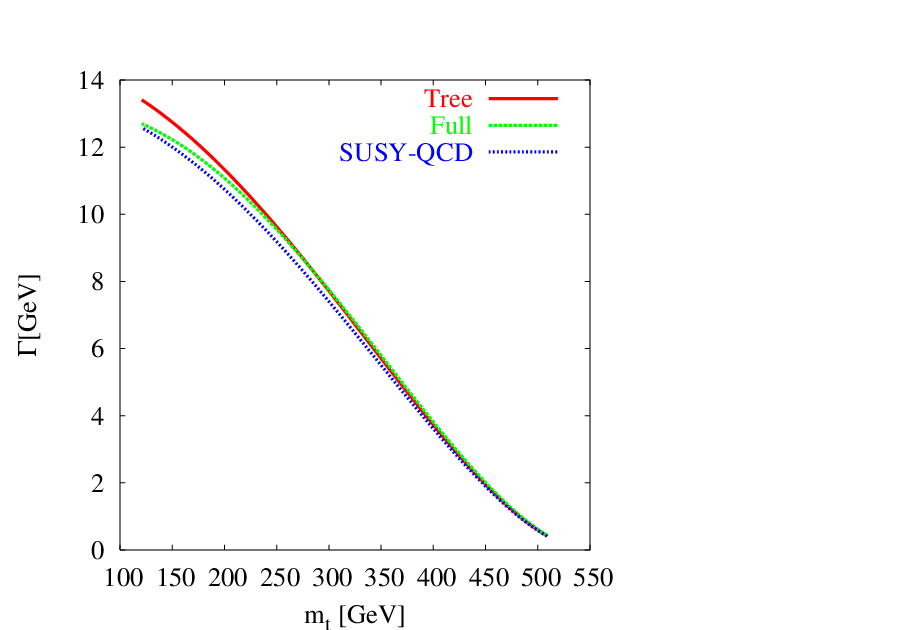
Finally, in Fig. (8) we illustrate the decay width of as function of in SPS1 (left) and SPS5 (right). In SPS1 (resp SPS5) the decay width of is about 8 GeV (resp 13 GeV) for light stop mass of the order 100 GeV. Obviously, these decays width decrease as the light stop mass increase.
It is clear that the SUSY-QCD corrections reduces the width while the electroweak corrections cancel part of those QCD corrections. Both in SPS1 and SPS5, the full one loop width of is in some case slightly bigger than the tree level width.
Conclusions:
A full one-loop calculations of third-generation scalar-fermion decays into gauge bosons W and Z are presented in the on–shell scheme. We include both electroweak, QED and SUSY-QCD contributions to the decay width. It is found that the QED corrections are rather small while the electroweak and SUSY-QCD corrections interfere destructively.
The size of the one-loop effects are typically of the order % in SPS scenarios which are based on SUGRA assumptions. While in model independent analysis like the general MSSM, the size of the corrections are bigger and can reach about 20% for large and large soft SUSY breaking . Their inclusion in phenomenological studies and analyses are then well motivated.
Acknowledgment:
The authors thanks ICTP for the warm hospitality extended to them during the first stage of this work. We thanks Margarete Muhlleitner for useful exchange of informations about Sdecay [23]. This work is supported by PROTARS-III D16/04.
References
- [1]
H.E. Haber and G.L. Kane, Phys. Rep. 117 (1985) 75;
H.P. Nilles, Phys. Rep. 110 (1984) 1;
P. Nath, R. Arnowitt and A. Chamseddine, “Applied N=1 Supergravity”, ITCP
Series in Theoretical Physics, World Scientific, Singapore 1984;
X.R. Tata, in Proceedings of the “Mt Sorak Symposium on the Standard Model and Beyond”, Mt Sorak, Korea, 1990 - [2]
T. Affolder et al. [CDF Collaboration],
Phys. Rev. D 63, 091101 (2001);
[arXiv:hep-ex/0011004].
G. Abbiendi et al. [OPAL Collaboration], Phys. Lett. B 545, 272 (2002) [Erratum-ibid. B 548, 258 (2002)] [arXiv:hep-ex/0209026]; - [3] F. del Aguila and L. Ametller, Phys. Lett. B 261 (1991) 326. H. Baer, C. h. Chen, F. Paige and X. Tata, Phys. Rev. D 49, 3283 (1994) [arXiv:hep-ph/9311248].
- [4] J. A. Aguilar-Saavedra et al. [ECFA/DESY LC Physics Working Group Collaboration], arXiv:hep-ph/0106315; K. Abe et al. [ACFA Linear Collider Working Group Collaboration], arXiv:hep-ph/0109166; T. Abe et al. [American Linear Collider Working Group Collaboration], in Proc. of the APS/DPF/DPB Summer Study on the Future of Particle Physics (Snowmass 2001) ed. N. Graf, arXiv:hep-ex/0106056.
- [5] W. Beenakker, R. Hopker, M. Spira and P. M. Zerwas, Nucl. Phys. B 492, 51 (1997) [arXiv:hep-ph/9610490]; W. Beenakker, R. Hopker, M. Spira and P. M. Zerwas, Phys. Rev. Lett. 74, 2905 (1995) [arXiv:hep-ph/9412272].
- [6] J. L. Feng and D. E. Finnell, Phys. Rev. D 49, 2369 (1994) [arXiv:hep-ph/9310211]; T. Tsukamoto, K. Fujii, H. Murayama, M. Yamaguchi and Y. Okada, Phys. Rev. D 51, 3153 (1995); R. Keranen, A. Sopczak, H. Nowak and M. Berggren, Eur. Phys. J. directC 2 (2000) 7; R. Kitano, T. Moroi and S. f. Su, JHEP 0212, 011 (2002) [arXiv:hep-ph/0208149]; E. L. Berger, J. Lee and T. M. Tait, arXiv:hep-ph/0306110.
- [7] A. Arhrib, M. Capdequi-Peyranere and A. Djouadi, Phys. Rev. D 52, 1404 (1995) [arXiv:hep-ph/9412382]. M. Drees and K. I. Hikasa, Phys. Lett. B 252, 127 (1990).
- [8] H. Eberl, A. Bartl and W. Majerotto, Nucl. Phys. B 472, 481 (1996) [arXiv:hep-ph/9603206].
- [9] A. Freitas et al., [arXiv:hep-ph/0211108]. A. Freitas, D. J. Miller and P. M. Zerwas, Eur. Phys. J. C 21, 361 (2001) [arXiv:hep-ph/0106198].
- [10] A. Arhrib and W. Hollik, JHEP 0404, 073 (2004) [arXiv:hep-ph/0311149].
- [11] H. Eberl, S. Kraml and W. Majerotto, JHEP 9905, 016 (1999) [arXiv:hep-ph/9903413]. K. Kovarik, C. Weber, H. Eberl and W. Majerotto, Phys. Lett. B 591, 242 (2004) [arXiv:hep-ph/0401092].
- [12] M. Beccaria, M. Melles, F. M. Renard, S. Trimarchi and C. Verzegnassi, [arXiv:hep-ph/0304110].
- [13] A. Djouadi, W. Hollik and C. Junger, Phys. Rev. D 55, 6975 (1997); S. Kraml, H. Eberl, A. Bartl, W. Majerotto and W. Porod, Phys. Lett. B 386, 175 (1996).
- [14] J. Guasch, W. Hollik and J. Sola, JHEP 0210, 040 (2002); J. Guasch, J. Sola and W. Hollik, Phys. Lett. B 437, 88 (1998);
- [15] A. Arhrib, A. Djouadi, W. Hollik and C. Junger, Phys. Rev. D 57, 5860 (1998) [arXiv:hep-ph/9702426].
- [16] A. Bartl, H. Eberl, S. Kraml, W. Majerotto, W. Porod and A. Sopczak, Z. Phys. C 76, 549 (1997) [arXiv:hep-ph/9701336].
- [17] W. Hollik and H. Rzehak, arXiv:hep-ph/0305328.
- [18] A. Bartl, H. Eberl, K. Hidaka, S. Kraml, W. Majerotto, W. Porod and Y. Yamada, Phys. Lett. B 419, 243 (1998) [arXiv:hep-ph/9710286].
- [19] B. C. Allanach et al., in Proc. of the APS/DPF/DPB Summer Study on the Future of Particle Physics (Snowmass 2001) ed. N. Graf, Eur. Phys. J. C 25, 113 (2002) [eConf C010630, P125 (2001)] [arXiv:hep-ph/0202233].
- [20] N. Ghodbane and H. U. Martyn, in Proc. of the APS/DPF/DPB Summer Study on the Future of Particle Physics (Snowmass 2001) ed. N. Graf, arXiv:hep-ph/0201233.
- [21] C. Kounnas, A. B. Lahanas, D. V. Nanopoulos and M. Quiros, Nucl. Phys. B 236 (1984) 438. J. F. Gunion, H. E. Haber and M. Sher, Nucl. Phys. B 306, 1 (1988). J. A. Casas, A. Lleyda and C. Munoz, Nucl. Phys. B 471 (1996) 3 [arXiv:hep-ph/9507294].
- [22] A. Djouadi, J. L. Kneur and G. Moultaka, arXiv:hep-ph/0211331.
- [23] M. Muhlleitner, A. Djouadi and Y. Mambrini, arXiv:hep-ph/0311167.
- [24] J. Kublbeck, M. Bohm, A. Denner, Comput. Phys. Commun. 60, 165 (1990); T. Hahn, Comput. Phys. Commun. 140, 418 (2001); T. Hahn, C. Schappacher, Comput. Phys. Commun. 143, 54 (2002); T. Hahn, M. Perez-Victoria, Comput. Phys. Commun. 118, 153 (1999);
- [25] G. J. van Oldenborgh, Comput. Phys. Commun. 66, 1 (1991); T. Hahn, Acta Phys. Polon. B 30, 3469 (1999)
- [26] W. Siegel, Phys. Lett. B 84, 193 (1979). D. M. Capper, D. R. Jones and P. van Nieuwenhuizen, Nucl. Phys. B 167, 479 (1980).
- [27] A. Denner, Fortsch. Phys. 41, 307 (1993).
- [28] W. Hollik, E. Kraus, M. Roth, C. Rupp, K. Sibold and D. Stockinger, Nucl. Phys. B 639, 3 (2002) [arXiv:hep-ph/0204350].
- [29] W. Majerotto, arXiv:hep-ph/0209137.
- [30] T. Fritzsche and W. Hollik, Eur. Phys. J. C 24, 619 (2002) [arXiv:hep-ph/0203159].
- [31] K. Hagiwara et al. [Particle Data Group Collaboration], Phys. Rev. D 66, 010001 (2002).
- [32]
S. Eidelman and F. Jegerlehner, Z. Phys. C67 (1995) 585–602.
D. Bardin et al., “Electroweak working group report”, in Reports of the Working Group on Precision Calculations for the Resonance, report CERN 95–03 (1995) (D. Bardin, W. Hollik, and G. Passarino, eds.), pp. 7–162, hep-ph/9709229.