hep-ex/0401034
nuhep-exp/04-01
Apparent Excess in
Michael Schmitt
Northwestern University
January 22, 2004
Abstract
We have studied measurements of the cross section for for center-of-mass energies in the range 20–209 GeV. We find an apparent excess over the predictions of the Standard Model across the whole range amounting to more than . As an example, we compare the data to predictions for a light scalar down-type quark which fit the excess well.
1 Introduction
Measurements of the inclusive cross section for have been a staple of collider experiments for many years. They have been essential for testing the predictions of QCD, and for measurements of the properties of the boson which underpin the electroweak sector of the Standard Model (SM). It is often said that the SM survives all confrontations with data, and indeed, this agreement is a very important constraint on models for new physics beyond the SM. For example, one of the strengths of the Minimal Supersymmetric extension of the Standard Model (MSSM) is the fact that it does not disturb this agreement though its parameters may be varied over wide ranges.
It has been noted several times that the Lep 2 measurements of tend to exceed the predictions of the SM [1]. It is also well known that the hadronic cross section at the peak, , slightly exceeds the SM fit [2, 3]. Neither of these excesses is statistically significant.
We have examined the data on from experiments that ran below the peak using a compilation amassed by Zenin et al., [4], and find that these measurements, taken together, also are in excess of the SM prediction. We developed a likelihood method to quantify the significance of the excess in four ranges of the center-of-mass energy, , and then combined the likelihoods. The net excess has a significance of over , if theoretical uncertainties and correlations for experimental systematic uncertainties are ignored. When a conservative theoretical uncertainty is applied, the significance reduces to , and when the correlations among experimental measurements are taken into account, the significance is , corresponding to a probability of .
We compare the data to three straw models of new physics: 1) a purely phenomenological ansatz with , 2) light bottom squarks () with little or no coupling to the , and 3) an additional neutral boson resonance () with a mass well beyond the energies of the data. We find that the data are consistent with a light , and do not favor an additional .
The structure of this report is as follows. First, we discuss the data used in this study, and then the SM prediction for . Next we compare the measurements to the SM prediction, which is based on the likelihood method. After establishing the excess on the basis of a very simple expression for any possible excess, we compare to the expectations for a light , and also to the expectation for a heavy . Finally, we draw our conclusions.
2 The Data
We base this analysis on data from the LepEWWG [2] and the compilation of measurements by Zenin et al. [4].
The results from the analysis of Lep data have been stable for some years. They fall naturally into two groups: measurements around the peak ( GeV) and well above ( GeV). We rely on the reports in Refs. [2, 3], both for the reduction of the measurements and for the SM predictions. A summary of the data is given in Table 1.
The data below the peak come from a number of experiments running at several colliders. The main interest in these data comes from the need for improved estimates of and corrections to . We consider two subsets, namely, GeV, for which -exchange should be unimportant, and GeV, which will show the onset of -exchange. The combined measurements in these two regions carry approximately equal precision. A summary of the relevant experiments is given in Table 2.
These considerations lead us to designate four regions based on :
| 1 | GeV |
|---|---|
| 2 | GeV |
| 3 | GeV |
| 4 | GeV |
We do not consider the data at GeV as some of these measurements are not very precise, the theoretical uncertainty from becomes large, and the prediction for any new particle might be complicated due to threshold effects. Plots of the data from regions 1, 2 & 4 are displayed in Figs. 1, 2 and 3.


There are 130 measurements for regions 1 & 2. The statistical precision of the typical measurement is , and the total systematic uncertainties are roughly the same as the statistical errors. In some cases the systematic uncertainties are not well described. Generally speaking, they involve the luminosity measurements, the hadronization model, and the trigger efficiency.
| energy | combined measurement | SM prediction | difference | deviation |
|---|---|---|---|---|
| 91.187 | ||||
| 130 | ||||
| 136 | ||||
| 161 | ||||
| 172 | ||||
| 183 | ||||
| 189 | ||||
| 192 | ||||
| 196 | ||||
| 200 | ||||
| 202 | ||||
| 205 | ||||
| 207 |
| experiment | (GeV) | publication |
|---|---|---|
| CELLO / PETRA | 34.9, 42.7 | Phys.Lett 144B (1984) 297 |
| 22.0, 33.8, 38.3, 41.5, 43.5, 44.2, 46.0, 46.6 | Phys.Lett 183B (1987) 400 | |
| JADE / PETRA | 22.0, 25.0, 27.7, 29.9, 30.4, 31.3, 33.9, 34.5, | |
| 35.0, 35.4, 36.4, 40.3, 41.2, 42.6, 43.5, 44.4, 45.6, 46.5 | Phys.Rep. 148 (1987) 67 | |
| 22.0, 27.6, 30.8 | Phys.Rep. 83 (1981) 151 | |
| Mark-J / PETRA | 31.6 | Phys.Lett. 85B (1979) 463 |
| 22.0, 27.6, 30.0, 30.7, 31.6, 33.0, 34.0, 35.3, 35.8 | Phys.Rep. 63 (1980) 337 | |
| 34.8 | Phys.Lett. 108B (1982) 63 | |
| 22.0, 25.0, 30.6, 33.8, 34.6, 35.1, 36.3, 37.4, 38.4, | ||
| 40.3, 41.5, 42.5, 43.5, 44.2, 45.5, 47.5 | Phys.Rev. D34 (1986) 681 | |
| TASSO / PETRA | 22.0, 27.7, 30.9, 31.6 | Z.Phys. C4 (1979) 87 |
| 22.0, 25.0, 27.6, 30.2, 31.0, 33.0, 34.0, 35.0, 36.0 | Phys.Lett. 113B (1982) 499 | |
| 22.0, 25.0, 27.7, 30.1, 31.5, 33.5, 34.5, 35.5, 36.7, 43.1 | Z.Phys. C22 (1984) 307 | |
| 41.4, 44.2 | Phys.Lett. 138B (1984) 441 | |
| 22.0, 35.0, 43.7 | Z.Phys. C47 (1990) 187 | |
| Mark-II / PEP | 29.0 | Phys.Rev. D43 (1990) 34 |
| MAC / PEP | 29.0 | Phys.Rev. D31 (1985) 1537 |
| AMY / TRISTAN | 50.0, 52.0, 54.0, 55.0, 56.0, 56.5, 57.0, 58.5, | |
| 59.0, 59.1, 60.0, 60.8, 61.4 | Phys.Rev. D42 (1990) 1339 | |
| TOPAZ / TRISTAN | 50.0, 52.0, 54.0, 55.0, 56.0, 56.5, 57.0, 58.3, | |
| 59.1, 60.0, 60.8, 61.4 | Phys.Lett. 234B (1990) 525 | |
| 57.4, 58.0, 58.2, 58.5, 58.7, 59.0, 59.2, 59.5, 59.8 | Phys.Lett. B304 (1993) 373 | |
| 57.8 | Phys.Lett. B347 (1995) 171 | |
| VENUS / TRISTAN | 50.0, 52.0 | Phys.Lett. 198B (1987) 570 |
| 63.6, 64.0 | Phys.Lett. B246 (1990) 297 |
3 Standard Model Predictions
The SM predictions for the inclusive process are relatively simple. Let be the mass of a particular quark, so is its velocity. Denote its electric charge by , and weak isospin by . The fundamental constants are the Fermi constant, , the QED coupling , and the strong coupling . The latter two run as a function of . Finally, the weak mixing angle relates weak and electric couplings, and can be defined according to
| (1) |
where is the mass of the boson. Since runs, so does , according to this definition. The vector and axial vector couplings of the quark to the can be written
| (2) |
and the propagator in the lowest order is simply [5]
| (3) |
where is the width.
The amplitude for is the sum of the amplitudes for and exchange, so the cross section is the sum of three terms. After integrating over all angles,
| (5) | |||||
where is a QCD correction factor depending on and the number of colors, .
Equation (5) pertains to the simple Born approximation when , and hence , are fixed, and . The improved Born approximation allows for running and , for finite corrections to , and for an energy dependent width: , with independent of . We list the values for all required constants in Table 3.
| parameter | value |
|---|---|
| MeV | |
| GeV | |
| GeV | |
| GeV | |
| GeV |
We use version 6.36 of the Zfitter program [6] to compute the SM predictions in regions 1 & 2. This program has been developed by several authors over many years, and is one of the two main programs employed by the LepEWWG. For an in-depth discussion of the theoretical accuracy of the predictions from Zfitter, see the paper by Bardin, Grünewald, and Passarino [7].
The routine for computing the -dependent hadronic corrections to was recently improved by Jegerlehner [8], who provided us with nearly-final version. We use this new routine for our SM computations. The change in is generally less than , and so the impact on the cross section is negligible.
We wrote our own code to compute the cross section for , based on Eq. (5). For we used a routine from H.Burkhardt [9], and for the QCD correction factor, , we used an expression published by S.Bethke [10]:
| (6) |
with and . The exact values of and depend slightly on the quark masses, and we consider the uncertainties of these coefficients below.
We compared the results of our code to those of Zfitter. There is agreement at the level of after accounting for the fact that the running of the heavy quark masses is implemented in Zfitter but not in our code; the predictions from Zfitter are slightly higher than those from our code at the level of –. Also, box diagrams contribute about to above the threshold, which is not included in the simple expression Eq. (5). For the comparison of the SM prediction to the data, we use the values from Zfitter, as this program is extremely well tested and reliable. Our code is useful for investigating sources of theoretical errors, as discussed below.
We must assess the uncertainty on the SM prediction in order to make the comparison to the data. The studies by Bardin et al. [7] indicate that the theoretical accuracy is 0.2% or better, in regions 1 & 2. For region 4, the Two-Fermion Working Group reports a theoretical uncertainty of 0.26% [11]. They also report values for which imply an uncertainty on of 0.14%, and we obtain similar results.
The uncertainty coming from the inputs must also be estimated. For , we must consider both the uncertainty on its measured value at , and the uncertainty from the running, which is dominated by the uncertainty on . The uncertainty from is negligible. We estimate the uncertainty from the running by modifying the coefficients in the Burkhardt routine to correspond to at the peak [9]. This is a conservative estimate and is the same used by the LepEWWG in their analyses of Lep data. Other estimates suggest a significantly smaller uncertainty [12]. Furthermore, we take the uncertainty from on the SM cross section to be fully , ignoring the fact that uncertainties will be smaller for the terms involving , as we have explicitly verified using our code based on Eq. (5).
The uncertainty coming from the QCD correction also has two pieces: the uncertainty on and the uncertainty on the coefficient . We do not consider an uncertainty on as this would be redundant with the uncertainty on . As discussed by S.Bethke [10], there is some spread in the values for coming from various sets of measurements. There is a tendency for the lower energy measurements, such as deep-inelastic scattering, to give a value of lower than that coming from the data at higher energy, mainly from Lep. A typical average is [10]. The central value is more or less mid-way between the low values favored by DIS measurements and the high values favored by Lep. In the context of the light sbottom model discussed below, will run more slowly resulting in a slightly higher value at [13]. We choose to keep the central value (), but double the uncertainty to . In the parametrization of the running of by Bethke [10], this corresponds to the low-energy parameter MeV. We evaluated the impact of this uncertainty on the SM cross section using our code and find it to be on the order of . We also varied the coefficient by 10% and found the impact to be negligible.
We evaluated the uncertainties coming from the other input parameters, namely, , , and , and found them to be completely negligible.
A summary of the theoretical uncertainties for the entire range of is given in Fig. 4. The dominant error comes from the running of , which has been very conservatively estimated. We display also the linear sum of the uncertainties, and use this as the guide for setting the theoretical uncertainty. For the range , we take an uncertainty on the order of 0.5%, which falls slightly from to , as indicated by the heavy line. For region 3, we do not include a theoretical uncertainty, as this parameter is a fit result, and the reported theoretical uncertainty is exceedingly small, amounting to , or [7]. In region 4, we take an uncertainty of , as indicated by the second heavy line.
We emphasize that these theoretical uncertainties are conservative, and one could argue that more agressive estimates closer to would be justified.

4 Comparison of the Data to the SM Prediction
We develop a series of comparisons, starting with a simple weighted average of differences and ending with a likelihood analysis which incorporates theoretical and experimental systematic uncertainties, and correlations among errors.
4.1 Mean Deviations
We compare the SM prediction to the data in each of the four kinematic regions defined above. First, we compute a simple and mean deviation of the data from the SM prediction. Let the measurements be with uncertainties , and the SM prediction, , which varies with . Then
| (7) |
and the mean deviation and rms are
| (8) |
At this point we ignore correlations among the measurements. We summarize the values for , and in Table 4. No value is given for region 3 as there is only one data point there. Note that the mean deviation is significantly non-zero and positive, even though the is fine. This is a key point and a somewhat atypical situation. There are many measurements, each of which is statistically consistent with the SM prediction, and so the value of is good. But the test does not distinguish between measurements which are higher than the prediction and those which are lower. In the present case, it turns out that there are many more which are higher than lower. The mean deviation, , is designed to make this evident. To demonstrate that these offsets are plausible, we form local averages of the data for regions 1 & 2, and plot the ratio of the rebinned data to the SM prediction – see Fig. 5. The likelihood analysis discussed in the next section provides a more physical basis for analyzing the apparent excess indicated by the values in Table 4.
| region | N data points | ||||
|---|---|---|---|---|---|
| 1 | 67 | 50.4 | 6.7 | 2.5 | 2.9 |
| 2 | 63 | 55.1 | 7.9 | 1.4 | 5.9 |
| 4 | 12 | 12.2 | 0.32 | 0.11 | 2.8 |

4.2 Simple Likelihood Analysis
We wish to quantify better any disagreement of the SM prediction with the data. To this end, we define a likelihood function, based on the measurements with uncertainties and the theoretical prediction, (SM + new physics), where is a free parameter,
| (9) |
It is understood that both and are functions of . It is more convenient to work with the negative log-likelihood function, . We will examine the change in as a function of .
The quantity represents a contribution from new physics. As the simplest ansatz, we take
| (10) |
which has the generic dependence of the pair production of light particles, and we normalize to 10 pb at for convenience later. In this case the influence of -exchange is ignored. Minimizing the negative log-likelihood function as a function of , we obtain the results () summarized in Table 5. One sees that a positive contribution is favored in all cases – this comes about because the mean deviations, are all positive (see Table 4). One also sees that ignoring -exchange does not appear to be justified, since is much larger for region 3 than for the others.
We compare the best values of to those obtained for the SM alone (i.e., with ) and see an improvement when a nonzero “new physics” contribution is included. This improvement can be described by a number of standard deviations (S.D.) according to
| (11) |
as discussed in the RPP, for example [14]. We checked that the minimization of and the interpretation of the error on corresponded exactly to what is obtained with a standard minimization, region by region.
| region | S.D. | |||
|---|---|---|---|---|
| 1 | 0.74 | 21.89 | 25.23 | 2.58 |
| 2 | 1.80 | 25.52 | 37.50 | 4.90 |
| 3 | 57.3 | 0 | 1.404 | 1.68 |
| 4 | 1.37 | 2.00 | 6.12 | 2.87 |
| net | 1.183 | 53.446 | 70.255 | 5.80 |
The values listed in Table 5 do suggest that there is an apparent excess of data over the SM prediction, in all four regions of . It makes sense to form a combined likelihood by taking the product of the likelihoods for the four regions. The corresponding negative log-likelihood function is then minimized with respect to the scale , with the result:
| (12) |
The difference in is 16.81, which corresponds to 5.8 standard deviations, according to Eq. (11).
The value Eq. (12) is significantly different from zero, but still is very small. It corresponds to only 3% of the hadronic cross section at . At this energy, the cross section for the production of a lepton pair is about , and for a charge quark, about . Interestingly, the cross section for a scalar particle will be significantly smaller, due to the reduced number of spin degrees of freedom.
4.3 Theoretical Uncertainties and Experimental Systematics
The theoretical uncertainties depicted in Fig. 4 are not negligible compared to the deviations in Table 4. Furthermore, we have taken the measurements to be uncorrelated, which is not the case. We now rectify these deficiencies and see to what extent the significance of the apparent excess diminishes.
To implement the theoretical uncertainties, we modify the likelihood function to include a multiplier, , for which is constrained by a Gaussian centered on one with a width given by the assumed theoretical uncertainty, :
| (13) |
where we have omitted unnecessary normalization factors. The likelihood and corresponding negative log-likelihood are to be viewed as functions of both the new physics scale factor, , and the scale factor for the SM prediction, . The second factor will allow a numerical improvement in the likelihood when , but will have no impact for the optimal . The result is a smaller difference and hence a lower significance.
We apply this new formulation of and find a significant reduction in , as expected. The significance is reduced from to .
Next we take into account the correlation among the measurements. For the Lep 2 data, this is straight forward, as the LepEWWG have published the covariance matrix [2]. For the lower energy data, no rigorous prescription is possible, so we adopt the following method. The data appear in twenty-one distinct publications, as listed in Table 2. It is reasonable to assume that the measurements reported in a given publication are correlated, so we take half the total systematic uncertainty to be correlated. Correlations among sets of measurements, however, are expected to be very small, since nearly all of the systematic uncertainties come from detector specific issues (such as the alignment of the luminosity detectors, or the measurement of the trigger efficiency), or are evaluated in different ways (such as the dependence on the hadronization model).
We replace the sum over individual terms in the negative log-likelihood function by one-half the formed in the canonical way from the inverse of the covariance matrix. This function depends on in the same way does. The data in regions 1 & 2 are treated together as part of one function, and the data in region 4 is treated in a separate function.
Since the weight of each measurement is different once correlations are taken into account, the net function must be minimized anew. Setting aside the theoretical uncertainties, the significance of the excess is reduced from to . Taking both the theoretical uncertainties and the correlations into account, we find a significance of .
5 Examples: Light Sbottoms, Extra Boson
For the sake of discussion, we take the apparent excess to be genuine and compare the data to two ansätze for physics beyond the SM:
- 1.
light bottom squarks
- 2.
heavy bosons
The first model serves as the example of the production of new light particle in collisions, while the second involves a new production mechanism of purely SM particles. They can be distinguished, in the absence of an analysis of the final state, by their dependence on : the one falls as while the other rises approximately as , far below the pole in the propagator. We do not mean to advocate either of these models, but rather use them as reasonable models to test with these measurements of . They are both well motivated by other considerations.
5.1 Light Sbottoms
The light sbottom model comes from the proposal by E.Berger et al. [15] to explain the excess of -hadron production at the Tevatron by postulating the existence of a light sbottom quark (), with a mass in the range , and a light gluino () with a mass of roughly . The gluino decays only to , and the sbottom decays via an -parity violating coupling to a pair of quarks: , for example. For our purposes, the gluino plays no role – we assume that these light these bottom squarks produce hadronic jets through an -parity violating coupling () which would allow them to be selected in the measurements of with approximately the same efficiency as a SM event . While the SM quarks have a substantial coupling to the boson, the composition of the lightest sbottom can be tuned so make this coupling arbitrarily small. In the case that it is exactly zero, the cross section would have the generic -dependence of Eq. (10). The composition is controlled by a mixing factor, , and zero coupling corresponds to . In our comparison of the light sbottom model to the data, we will have to allow to be a free parameter. It is known from a comparison to the total width, however, that [16]. We use the code Msmlib from G.Ganis to compute the sbottom cross sections [17], and fix the sbottom mass to .
To examine the dependence of on , we first fix . A shown below, this is close its optimal value. The results of the minimization of are as one would expect. The first region is dominated by photon exchange, and so there is no sensitivity to . The second retains a very mild sensitivity to , favoring , since the excess in this region is large. Region 3 is dominated by exchange, and so the dependence of the cross section on is strong. It clearly favors a reduced coupling to the , and the limit is easily obtained. Finally, the data from region 4 have a mild sensitivity to , similar to what is seen for region 3.
We sum the negative log-likelihood functions for the four regions and plot the sum as a function of , as shown in Fig. 6. This variation is dominated by the pole data. The preferred value is , which gives a small but non-zero coupling to the , as required by the small excess in . A zero coupling corresponds to , and is not excluded by the data – it is disfavored by only 1.3 standard deviations.

We now fix , and return to the procedure to evaluate the significance of the excess as described in the last section. Specifically, we allow for an overall theoretical uncertainty, and we take correlations among measurements into account. In the present context we are comparing the quality of the description of the data for SM + a light sbottom to the SM alone. We vary freely for the sum of negative log-likelihoods, and obtain for which , to be compared to . In the latter case, the systematic uncertainty on the SM prediction allows an enhancement of the prediction by 0.87% – i.e., in Eq. (13). This difference in corresponds to standard deviations, for a probability of .
It is important to note the following three points:
- 1.
All four regions contribute positively to at .
- 2.
The best overall point, , is not disfavored by any of them, and is statistically consistent with the best point for each individual region.
- 3.
The best overall point is consistent with .
To illustrate these points graphically, we temporarily revert to the definitions of which neglect theoretical uncertainties and correlations, and plot the variation of for each of the four regions and their sum – see Fig. 7.
The minima of the four parabolas fall closer to than to . This indicates there is a consistent excess in all four regions. The sum of the four parabolas has a sharper minimum at . The rise in the negative log-likelihood passing from to corresponds, when interpreted as a number of standard deviations, to . (Recall that, after taking theoretical uncertainties and correlations among measurements into account, this number is reduced to .) In this sense one can say that the data prefer a description which includes a light sbottom, with a high level of statistical significance. If the parabola were centered at instead, one would say that this model for a light sbottom is excluded. However, one cannot say that the data exclude the Standard Model. The contribution to of SM processes is indisputable, while the contribution from light sbottoms is speculative. The results of this analysis do not prove the existence of light sbottoms, rather, they suggest there may be new processes contributing to the hadronic final state.

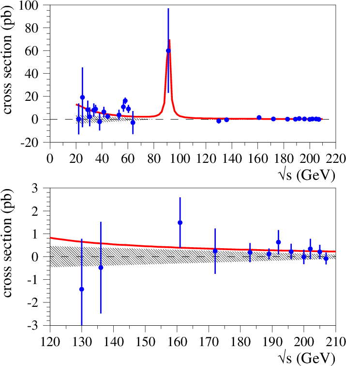
For illustration, we plot the difference between the rebinned measured values and the SM prediction as a function of , as shown in Fig. 8. The shaded band centered on zero indicates the conservative error we have assigned to the SM prediction. The heavy smooth curve indicates the cross section for a light sbottom () when .
5.2 A Heavy Boson
We consider the exchange of a third boson, call it , in the process . For simplicity, we assume that there is no interference between this and the photon and SM boson. If the mass of this , , were much higher than the probed by these measurements, then cross section would rise approximately linearly in :
| (14) |
The factor contains the coupling and other factors.
We use the expression Eq. (9) with . A summary of the results for the four regions is given in Table 6. The combined likelihood gives , for a , corresponding to 2.8 standard deviations. This model makes only a small improvement over the SM. The rising dependence pits the Lep 2 data against the data in regions 1 & 2 – one has either too high in region 4 or too small in regions 1 & 2. This model is distinctly less successful than the other two.
| region | S.D. | |||
|---|---|---|---|---|
| 1 | 0.50 | 21.89 | 25.23 | 2.58 |
| 2 | 0.27 | 17.31 | 37.50 | 6.35 |
| 3 | 0.67 | 0 | 1.404 | 1.68 |
| 4 | 0.0007 | 2.46 | 6.12 | 2.70 |
6 Summary
We have examined the measurements of across a wide range of energies and experiments. None of these measurements shows a significant excess over the predictions of the Standard Model. Taken together, however, there is a clear trend, which has been quantified in a number of ways.
Motivated by this apparent excess, we compared the data to a model for the production of light scalar -quarks, of the type suggested by the Argonne group [15]. As a specific example, we have considered sbottoms with a mass of and a mixing of left- and right-states parametrized by . This mixing gives a relatively small but non-zero coupling to the boson.
When all measurements are taken to be independent, and when theoretical uncertainties in the SM prediction are ignored, the light sbottom model is ‘preferred’ over the SM by . When correlations among measurements are taken into account, this significance drops to . Finally, when a very conservative theoretical uncertainty is folded into the calculation, the resulting significance is , which corresponds to a probability of .
Alternative models are less successful in describing the data. A new neutral gauge boson is disfavored, and a cross section with a generic dependence does not explain the slight excess at Lep 1 (though it still provides an improvement over the SM with a significance of ).
We conclude that the description of the data on is significantly improved if Standard Model processes are augmented by the pair production of light scalar particles of charge which appear as hadronic final states.
Acknowledgments
I am very grateful to André de Gouvêa for many stimulating discussion through the course of this study. I also acknowledge helpful discussions with Ed Berger, Marcela Carena, Martin Grünewald, Fred Jegerlehner, Zack Sullivan, Tim Tait, Mayda Velasco and Carlos Wagner. This work was supported by US DoE contract DE-FG02-91ER40684.
References
- [1] Jens Erler, “Constraining Electroweak Physics,” hep-ph/0310202; Guy Wilkinson, “LEP 2 : Results and Interpretations,” hep-ex/0205103; Stephen Wynhoff, “Standard Model Physics Results from LEP 2,” hep-ex/0101016
- [2] The Lep Collaborations and the LepEWWG, “A Combination of Preliminary Electroweak Measurements and Constraints on the Standard Model,” hep-ex/0312023
- [3] The Lep Collaborations and the LepEWWG, “Combination Procedure for the Precise Determination of Boson Parameters from the Results of the LEP Experiments,” hep-ex/0101027
- [4]
O.V.Zenin et al.,
“A Compilation of Total Cross Section Data on
hadrons and pQCD Tests,”
hep-ph/0110176
These data are quoted by the Particle Data Group
in their cross section plots – see
http://pdg.lbl.gov/2002/contents_plots.html.
We downloaded the data files directly from the web site
http://wwwppds.ihep.su:8001/comphp.html. - [5] G.Altarelli, R.Kleiss and C.Verzegnassi, eds., Physics at LEP 1, Chapter 1: “Electroweak Radiative Corrections for Physics,” CERN 89-08
- [6] D.Bardin et al., “ZFITTER v.6.21 - A Semi-Analytical Program for Fermion Pair Production in Annihilation,” Comput.Phys.Commun. 133 (2001) 229-395 hep-ph/9908433 We used version 6.36, augmented by an improved treatment of the – see [8].
- [7] Dmitri Bardin, Martin Grünewald, and Giampiero Passarino, “Precision Calculation Project Report,” hep-ph/9902452
- [8]
Improved treatment of , called had5n.f,
sent by F. Jegerlehner at
http://www-zeuthen.desy.de/fjeger/ - [9]
H.Burkhardt and B.Pietrzyk,
Phys.Lett. B513 (201) 46-52
We downloaded the routine repi2001.f from the public web page
http://home.cern.ch/hbu/aqed/ - [10] S. Bethke, “Determination of the QCD Coupling ,” J.Phys. G26 (2000) R27 hep-ex/0004021
- [11] The Two-Fermion Working Group, Michael Kobel and Zbigniew Was, eds., “Two-Fermion Production in Electron-Positron Collisions,” hep-ph/0007180
- [12] K.Hagiwara et al., “Predictions for of the muon and ,” hep-ph/0312250; F.Jegerlehner, “Theoretical Precision in Estimates of the Hadronic Contributions to and ,” hep-ph/0310234 The paper from Hagiwara et al. reports and Jegerlehner reports , to be compared to the value we use, [9].
- [13] Cheng-Wei Chiang, Zumin Luo and Jonathan Rosner, “Light Gluino and the Running of ,” Phys.Rev. D67 (2003) 035008 hep-ph/0207235
- [14]
The Review of Particle Physics:
K.Hagiwara et al., Phys.Rev. D66 (2002) 010001 - [15] E.L.Berger, B.W.Harris, D.E.Kaplan, Z.Sullivan, T.Tait and C.E.M.Wagner, “Low-Energy Supersymmetry and the Tevatron Bottom-Quark Cross Section,” Phys.Rev.Lett. 86 (2001) 4231-4234
- [16] M.Carena, S.Heinemeyer, C.E.M.Wagner and G.Weiglein, “Do Electroweak Precision Data and Higgs-Mass Constraints Rule Out a Scalar Bottom Quark with Mass of Order 5 GeV?” Phys.Rev.Lett. 86 (2001) 4463
- [17]
A library for calculating MSSM cross sections, masses
and branching ratios:
G.Ganis, msmlib, http://alephwww.cern.ch/ganis/MSMLIB/msmlib.html