Symmetries and assisted inflation in the DGP braneworld model
Abstract
We present here the general transformation that leaves unchanged the form of the field equations for perfect fluid cosmologies in the DGP braneworld model. Specifically, a prescription for relating exact solutions with different equations of state is provided, and the symmetries found can be used as algorithms for generating new cosmological models from previously known ones. We also present, implicitly, the first known exact DGP perfect fluid spacetime. A particular case of the general transformation is used to illustrate the crucial role played both by the number of scalar fields and the extra dimensional effects in the occurrence of inflation. In particular, we see that assisted inflation does not proceed at all times for one of the two possible ways in which the brane can be embedded into the bulk.
1 Introduction
Over the last years the brane world scenario has aroused an overwhelming curiosity (see [1] and references therein). According to that idea our 4D universe lives on a domain wall embedded in a manifold with an extra spatial dimension, so that gravity, but not standard models fields, can spread into this additional dimension. In what cosmological implications are concerned, most attention has been devoted to the Randall Sundrum (RS) II scenario [2], which has recently faced the rise of a challenger for the title of the cosmologists’ preferred brane cosmology model: the alternative scenario proposed by Dvali, Gabadadze and Porrati (DGP) [3]. In those two models the extra dimension is infinitely large. The DGP proposal rests on the key assumption of the presence a four-dimensional Ricci scalar in the action. There are two main reasons that make this model phenomenologically appealing. First, it predicts that 4D Newtonian gravity on a brane world is regained at distances shorter than a given crossover scale (high energy limit), whereas 5D effects become manifest above that scale 11 1 If the successful predictions of ordinary cosmology are to be preserved, the crossover scale must be of the order of the Hubble scale today. (low energy limit). Second, the model can explain late-time acceleration without having to invoke a cosmological constant or quintessential matter. Interestingly enough, the only way to mimic such scenario in a purely 4D is to introduce in the Einstein-Hilbert action covariant terms with fractional powers of the Ricci scalar [4]. Since that seems unjustifiable at present, cosmic acceleration in the model is regarded as an intrinsically high-dimensional effect.
Geometrical aspects of the model have been studied in [4, 5], and we will briefly review them in Section 2. In connection with this, the remark must be done two different solution sets arise depending on how the brane is embedded into the bulk, the discrepancy the sign in one of the terms in the modified Friedmann equation.
Other studies have focused on cosmological consequences [6, 7, 8]. In this work mathematical and physical aspects will overlap: First, in Section 3 we will formally show how, by exploiting symmetry properties, one can relate different exact solutions to the evolution and conservation equations equations describing perfect fluid FRW spacetimes in the DGP model. The procedure will establish the link between cosmologies with different equations of state, and can be thought of as an unusual solution generating algorithm. It must be stressed that, by construction, the new scale factor, Hubble factor, energy density and pressure will satisfy the same evolution and conservation equations as the seed model, and so such set of scalar quantities represent our transformed solution.
Next, in Section 5 we will apply our method to the generation of inflationary solutions from non-inflationary ones. Specifically, the energy density of the transformed model will be a number of times larger than the original one, in the fashion of assisted inflation [9]. When applied to inflationary solutions, provided the energy density of the transformed model is large enough, those transformations will give solutions with faster expansion or slower expansion, depending on which branch of solutions is being considered. Obviously, only in the case in which expansion is enhanced it will be possible to say that we have a realization of the assisted inflation phenomenon. Then, a somehow unwanted effect of the fifth dimension is that an increase in the energy density does not generically result in more acceleration.
Our discussion of assisted inflation is grounded on the same procedure as in earlier papers [10], but the reader may also be interested in looking at the different views on brane assisted inflation taken in [12]. Interestingly enough, assisted inflation produced by tachyonic instead of standard scalar fields has also been considered [13].
The possibilities of the method will be illustrated with exact examples. In particular, we will consider exact perfect fluid FRW cosmologies. Remarkably, exact DGP cosmologies have not appeared in the literature before. Note, anyway, that the fact the solutions we present can only be given implicitly does not make them less illustrative. For completeness, we will discuss the asymptotic behaviour of the solutions, and establish comparisons with related works. After that, we will apply the aforementioned transformations which relate inflationary and non-inflationary solutions, and will explicitly discuss in detail under which circumstances assisted inflation occurs.
Finally, we will outline our main conclusions in Section 6.
2 Basic equations and main features
We now concentrate on the dynamics of a brane-world filled a perfect fluid with energy density and identical pressure along the three spatial directions (isotropic perfect fluid). The model is governed by the Friedmann equation [7]
| (1) |
and the energy conservation equation
| (2) |
where, is the Hubble factor, as usual. Although the model can be generalized to include a non trivial brane tension and a 5D cosmological constant, we will stick with our simplified picture. Since The second term in the r.h.s. of (1) can either be positive or negative, depending on how the brane is embedded into the bulk, we will be dealing with two branches of solutions [7]. We will refer to them as to the and the branch respectively, and wherever some term in a equation can take different signs it must be understood that the upper one corresponds to the branch.
The modified Friedmann equation is not as easy to handle as its relativistic version, it is convenient to define an effective energy density so that
| (3) |
From equations (2)–(3) and we obtain the Raychaudhuri equation
| (4) |
Obviously, the cosmological dynamics is bound to be influenced by quantum corrections, although, interestingly, the modifications are not relevant in all energy regimes. Needless to say, since in most expanding models the energy density decreases in the course of expansion, typically, high and low energy regimes correspond to early and late times, respectively. At early times, it follows that
| (5) |
so we see situation is the same as in general relativity (GR). In contrast, DGP and GR late-time dynamics are substantially different. Indeed, for matter that redshifts faster than curvature it can be seen that
| (6) |
In the branch, any expanding model evolves into a de Sitter phase and inflation is guaranteed at late times. This is a striking feature of the model because it provides a possible answer for the currently observed acceleration, without having to resort to dark energy. In the branch we find that late time expansion is also faster than in the relativistic setup, and, therefore, the conditions for the occurrence of inflation are less restrictive. If we speak in terms of perfect fluids, inflation depends on the value of the ratio of the model, but if we want to express the same idea using scalar fields and potentials, then we will say that the occurrence of accelerated expansion depends on how steep the potential is. In general, one needs fairly flat potentials for inflation to proceed.
In the relativistic setup, the assisted inflation proposal [9] came to change those views: If the universe is filled with a single field and its potential is very steep, inflation may not occur, but if there are many of those fields inflation the situation may get reversed, and inflation may occur, the only requirement being a large enough number of such fields. In other words, the cooperation of scalar fields with potentials not flat enough to produce inflation on their own, may result in enough effective potential energy for accelerated expansion. The specific models used for illustrating that idea considered FRW universes filled with sets of identical fields with identical self-interaction potentials, thus, the effective energy density of the model would be times the energy density of a single field. Correspondingly, the Hubble factor would get multiplied by [11]. Almost a decade ago, Barrow and Parsons [14] noticed the existence of this particular form-invariance transformation of the Einstein-Klein-Gordon equation system, although there the result was neither interpreted in terms form-invariance nor of assisted inflation.
This suggests that assisted inflation may be equally successful beyond general relativity. For instance, that has been proved to be the case in the Randall-Sundrum model. Now, we give one further step and show in the next section that it also may also apply to the DGP model, provided certain conditions hold.
3 Form-invariance transformations
Our main purpose is to show how the scale factor changes when the energy density of matter gets multiplied by a numerical factor. Given that the energy density is a function of the scale factor, the whole transformation comes down to a suitable change in the scale factor. Note that the transformation must meet the consistency criterion that the transformed quantities correspond to another exact solution of the gravitational field equations. The discussion, however, will be not restricted to any particular transformation. We will rather find out how the energy density, pressure, Hubble factor and deceleration factor get modified under an arbitrary change in the scale factor subject to the requirement that the transformation leaves invariant the field equations 22 2 We insist on the fact that this is another way of saying that the transformed cosmological model will be a solution of those equations.
We begin by considering a perfect fluid with energy density and pressure , which is governed by equations (1)–(2). Given a different perfect fluid with energy density and pressure , the corresponding equations will take the form
| (7) |
| (8) |
As said above, the objective is to obtain a transformation that leaves the form of the system of equations (7)–(8) unchanged. Put another way, we want to find a symmetry transformation that maps (7)–(8) into (1)–(2). Since we mean to obtain this transformation explicitly, we make the Ansatz
| (9) | |||||
| (10) | |||||
| (11) | |||||
| (12) |
The transformed versions of the last two equations can be obtained if we introduce an effective transformed energy density . We then get
| (13) |
and
| (14) |
In the procedure we are going to follow, we will regard as symmetry transformations those which do not impose restrictions on the functions appearing in the equations. When differentiating Eq. (10), a term proportional to arises, but such term must vanish identically, so that when we insert that expression in the l.h.s. of Eq. (14) we get a new expression consistent with the absence of terms proportional to in the r.h.s. of the same equation. Then, necessarily . If we replace now Eqs. (9) and (11) in Eqs. (7) and (8), and do the same reasoning, we draw the conclusion that and .
The next step is to calculate from Eq. (9) using the definition , so that
| (15) |
where equations (2) and (4) have been used. Since does not depend on , the coefficient of in Eq. (15) must vanish as well. For that reason,
| (16) |
and the general solution to the latter is , that is, depends on only.
Summarizing, the transformation turns out to be
| (17) |
| (18) |
| (19) |
| (20) |
where has to be calculated using Eq. (18). Clearly, once the prescription is made the symmetry transformation gets completely determined. Note that Eqs.(17)-(20) have been deduced without making any assumption on the equation of state of the fluid.
4 Inflation from form-invariance
Stages of accelerated expansion are marked by negative values of the deceleration parameter
| (22) |
Alternatively, one can write
| (23) |
which, upon specific knowledge of , allows to say whether for given and inflation occurs. Safely, in the GR case the requirement reduces to the violation of the strong energy condition .
The transformation rule for is to be deduced from (18) or (21) depending on whether we are considering cases with curvature or not, and in general one will obtain a complicated expression. Nevertheless, if we restrict ourselves (as we will in what follows) to cases in which , then (18) will hold both in the curved and non-curved cases, and it can be seen that
| (24) |
Let us concentrate for a moment on the case. Application of our transformation procedure which, in principle, be able to tell us which rule gives some some desired behaviour in either , , or a related quantity. In previous works, we were concerned with the case in which was a number of times larger than , that is , because that would mean that a non-inflationary solution would be transformed into an inflationary one for a conveniently chosen proportionality factor . Clearly, that situation arises when .
Alternatively, in the case, one starts by saying which is the relation between and so that we reproduce some behaviour of our choice. Note that it is not possible to make a priori assumptions on the link between and , one rather has to find it by integration. Provided is a known function of consistent with the energy conservation equation, and once the functional dependence between and has been specified, expressions of and in terms of would have to inserted in (18) to yield an ordinary differential equation with and as dependent and independent variables respectively. Integration of the latter would finally provide the rule leading to the pursued behaviour.
Roughly speaking, that approach to the problem we just discussed was, in fact, the way in which assisted inflation was analyzed originally. As said above, in [9] it was studied how the deceleration factor changes under the multiplication by a numerical factor of the energy density of the scalar fields driving inflation.
For the sake of simplicity we are concentrating on flat models (). It follows that, in order to have , one needs
| (25) |
where integration constants has been fixed so that and , and because of those choices
| (26) |
If we now insert (25) in (19) and (20), we would obtain the transformation rule for the energy density and pressure.Since in the DGP model the Friedmann equation is not linear in ,even though we are a case in which depends linearly on will not have a linear dependence on ; except in the high energy regime ().
In the next section , we will turn to explicit examples, and will discuss whether assisted inflation proceeds. Neverthelss, at this stage, we have enough information so as to discuss in broad terms whether our transformation enhances expansion or not. Eq. (25) was obtained upon integration of
| (27) |
which in turn was obtained by setting in (18). Let us assume . It can be seen that for . In contrast, for the branch . When the seed solution reaches the de Sitter phase (,), so does the trasfomed solution. One can see that the transition from being closer to (relativistic regime) than to (de Sitter regime) occurs at , and we infer the result that the larger the larger the value of at which the transition occurs. In general, we see that the expansion rate gets increased with the transformation in both branches, but the effect in more accentuated in the branch.
5 Explicit examples
So far, the discussion in this section has been carried out from a very broad perspective. It is time now to come to examples, and we choose the illustrative case. From the energy conservation equation it follows that
| (28) |
being an arbitrary integration constant. In the case exact solutions to the Friedmann equation can be given in the form :
| (29) |
where we have introduced a new variable for economy in the expressions. Remarkably, exact solutions to equations (1) and (2) have not appeared in the literature before.
Let us discuss now some aspect of the asymptotic kinematics of the solutions. The extra dimensional effects do not show up at early times (high energy regime), and, regardless of the branch, we have
| (30) |
together with , which is exactly the same result and in the relativistic framework. In contrast, at late times extra dimensional effects show up and give different solutions arise. For the branch we get
| (31) |
and . This is, of course, the solution found by Deffayet in [7], which is self-inflationary because accelerated expansion proceeds with a null energy density. For the branch we get
| (32) |
and , and the condition for inflation becomes , which is less restrictive than the relativistic condition ().
Obviously, asymptotic results are very relevant, but one may also be interested in the behaviour of the deceleration factor at any other time. In principle, it should be evaluated using (22), but because that is not an invertible expression, we have to resort to yet one more alternative definition of , namely
| (33) |
where ′ denotes differentiation with respect to . We then obtain
| (34) |
Combining (24) and (34) one can obtain , which is a complicated expression made of two terms. The first one (see (24)) is proportional to
| (35) |
which is smaller than provided , whereas the other term is exactly
| (36) |
In the branch, and for , (36) is strictly negative, and it follows, then, that
| (37) |
and the transformed model accelerates faster than the original one.
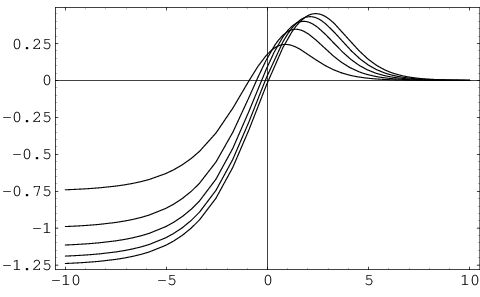
However, the situation is not so clear cut for the branch, because in that case for (36) is strictly positive. A series expansion in powers of indicates that for , but may occur at later evolution stages. In Fig. 1 we have plotted as a function of for . As can be seen, it agrees with our conclusion that is the rule at early times but does not hold at late times. Consistently, the figure also reflects the fact that , because all models end up in a de Sitter phase. Note that the peak in Fig. 1 which marks the transition between growing and decreasing , moves to the right (to larger values of the energy density) as grows, exactly as happens to the value which marks the transition from being closer to (relativistic regime) than to (de Sitter regime).
6 Conclusions
In this paper we have discussed form-invariance transformations in the setup of DGP brane cosmology. Specifically, we have found the transformation rules for the scalar magnitudes that characterize the dynamics of perfect fluid cosmologies so that a seed exact solution to the corresponding field equations is mapped into a new exact solution. The transformation is rather general, in the sense that it may be applied to any FRW cosmology (with or without curvature), regardless of the form of the Friedmann equation, which depends on the theoretical framework under consideration. As particular cases it includes, then, the transformations obtained in [11, 10].
Such transformation can be used, for instance, towards generating new exact solutions. In particular, one can construct inflationary cosmologies taking noninflationary seeds. Depending on how the brane-world is embedded into the fifth dimension, two solutions sets arise, the so called and branches.
We turn to consider then models with a barotropic equation of state. We explicitly construct the corresponding exact solution and then stick with it in the subsequent discussion. In general, an increase in the energy density, will give faster expansion in the branch, but in the other one, the contrary may happen. If the energy density is associated with a scalar field (the inflaton), and we think of an increase in it as being linked to a larger number of inflatons, we can safely speak of assisted inflation in the branch, very much like in the relativistic setup. However, this is not the case in the branch, and we see then that extra-dimensional effect make assisted inflation non-generic. In particular, in the branch assisted inflation only works at early times.
Summarizing, we have shown once again how important a role form-invariance transformations can play in the analysis and interpretation of exact solutions.
Acknowledgements
Thanks to J.M. Aguirregabiria, J.A. Valiente Kroon, and S. Jhingan for comments and suggestions. This work has been carried out with the support of the Basque Government through fellowship BFI01.412, the Spanish Ministry of Science and Technology jointly with FEDER funds through research grant BFM2001-0988, and the University of the Basque Country through research grant UPV00172.310-14456/2002.
References
- [1] R. Maartens, gr-qc/0312059; R. Maartens, Phys. Rev. D 62, 084023 (2000); D. Langlois, Astrophys Space Sci. 283, 469 (2003); Ph. Brax and C. van de Bruck, Class. Quant. Grav. 20, R201 (2003).
- [2] L. Randall and R. Sundrum, Phys. Rev. Lett. 83, 3370 (1999).
- [3] G. Dvali, G. Gabadadze and M. Porrati, Phys. Lett. B 484, 112 (2000); G. Dvali and G. Gabadadze, Phys. Rev. D 63, 065007 (2001); G. Dvali, G. Gabadadze, M. Shifman, Phys. Rev. D 67 (2003) 044020.
- [4] C. Deffayet, G. Dvali, and G. Gabadadze, Phys. Rev. D 65, 044023 (2002).
- [5] G. Dvali, G. Gabadadze, M. Kolanović, and F. Nitti, Phys. Rev. D 64, 084004 (2001); G. Kofinas, J. High Energy Phys. 0108, 034 (2001); C. Deffayet, Phys. Rev. D 66 103504 (2002); C. Deffayet, G. Dvali, G. Gabadadze, and A. Vainshtein, Phys. Rev. D 65 044026 (2002); G. Kofinas, E. Papantonopoulos, I. Pappa, Phys. Rev. D 66, 104014 (2002); G. Kofinas, E. Papantonopoulos, V. Zamarias, Phys. Rev. D 66 104028 (2002); S.L.Dubovsky, V.A.Rubakov, Phys.Rev. D67 104014 (2003); A. Lue, Phys. Rev. D 67, 064004 (2003).
- [6] C. Deffayet, Phys. Rev. D 66, 103504 (2002); A. Lue and G. Starkman, Phys. Rev. D 67, 064002 (2003).
- [7] C. Deffayet, Phys. Lett. B 502 199 (2001).
- [8] H. Collins, B. Holdom, Phys.Rev. D 62 105009 (2000); Y. Shtanov, hep-th/0005193; N. J. Kim, H. W. Lee, Y. S. Myung, Phys. Lett. B, 504, 323 (2001); V. Sahni and Y. Shtanov, Int. J. Mod. Phys. 11, 1 (2002); C. Deffayet, Phys. Rev. D 66, 103504 (2002); C. Deffayet, S.J. Landau, J. Raux, M. Zaldarriaga, and P. Astier, Phys. Rev. D 66, 024019 (2002) A. Lue and G. Starkman, Phys. Rev. D 67, 064002 (2003).
- [9] A.R. Liddle, A. Mazumdar, and F.E. Schunck, Phys. Rev. D 58, 061301 (1998).
- [10] J. M. Aguirregabiria et al., Phys. Rev. D 67, 083518 (2003); L. P. Chimento and R. Lazkoz Phys. Rev. Lett. 91, 211301 (2003).
- [11] L. P. Chimento, Phys. Rev. D 65, 063517 (2002).
- [12] L.E. Mendes and A. R. Liddle, Phys. Rev. D 62, 103511 (2000); A. S. Majumdar, Phys. Rev. D 64, 083503 (2001); Y.S. Piao et al., Phys. Lett. B 528, 188 (2002).
- [13] M. Sami, P. Chingangbam, and T. Qureshi, Phys. Rev. D 66, 043530 (2002);Y.S. Piao et al., Phys. Rev. D 66, 121301 (2002).
- [14] J.D. Barrow and P. Parsons, Class. Quantum Grav. 12, 1715 (1995)