跳到论文正文
W Papers独立论文阅读器 arXiv:cs/0703120 论文正文 计算阅读时间 · 0%
引用这篇论文根据当前论文元数据生成,正式投稿前建议核对。


License: Assumed arXiv.org perpetual non-exclusive license
arXiv:cs/0703120v1 [cs.IT] 23 Mar 2007

Sequential decoding for lossless streaming source coding with side information

Hari Palaiyanur       Anant Sahai    Thanks: This work was supported by the Vodafone US Foundation. Thanks: H. Palaiyanur and A. Sahai are with the Electrical Engineering Department at the University of California, Berkeley.
Abstract

The problem of lossless fixed-rate streaming coding of discrete memoryless sources with side information at the decoder is studied. A random time-varying tree-code is used to sequentially bin strings and a Stack Algorithm with a variable bias uses the side information to give a delay-universal coding system for lossless source coding with side information. The scheme is shown to give exponentially decaying probability of error with delay, with exponent equal to Gallager’s random coding exponent for sources with side information. The mean of the random variable of computation for the stack decoder is bounded, and conditions on the bias are given to guarantee a finite ρt​h\rho^{th} moment for 0≤ρ≤10\leq\rho\leq 1. Further, the problem is also studied in the case where there is a discrete memoryless channel between encoder and decoder. The same scheme is slightly modified to give a joint-source channel encoder and Stack Algorithm-based sequential decoder using side information. Again, by a suitable choice of bias, the probability of error decays exponentially with delay and the random variable of computation has a finite mean. Simulation results for several examples are given.

Index Terms: 
Data compression, side information, joint source-channel coding, sequential decoding, lossless source coding, Slepian-Wolf, error exponent, delay universal, stack algorithm, random variable of computation

I Introduction

In this paper, we consider the problem of lossless source coding with side information shown in Figure 1. The seminal paper of Slepian and Wolf [1] was the first to give the achievable rate region for this problem, when the source consists of a pair of dependent random variables that are independent and identically distributed (IID) over time. A sequence of IID symbols is encoded and its compressed representation is given noiselessly to a decoder. The decoder also has access to side information that is correlated in a known way with the source. The side information generally permits the source to be compressed to a rate below its entropy and still recovered losslessly. If the source is UU and the side information VV, then [1] showed that the conditional entropy, H⁡(U|V)H(U|V), is a sufficient rate to recover the UU with arbitrarily low probability of error.

Fig. 1: Source coding with side information at rate RR bits per time unit.

The currently known, robust methods of compression used in point-to-point lossless source coding generally employ variable length codes. Solutions such as Lempel-Ziv coding ([2], [3], [4]) and context-tree weighting [5] are also capable of efficiently compressing many sources with memory. Recently, these algorithms have been adapted to the ‘compression with side information’ problem when the side information is available to both the encoder and decoder. Cai, et al. [6] have shown how to modify the context-tree method to account for side information at the encoder. It is also possible to modify the Lempel-Ziv algorithms to account for side information at the encoder ([7], [8]).

The purpose of this paper, however, is to consider how to compress when the side information is available to the decoder only. This restriction disallows variable length codes as a generic solution. Variable length codes work because they assign short codewords to typical source strings and longer codewords to atypical strings. When the side information is available only to the decoder, the encoder cannot tell when the joint source is behaving atypically. As an example consider a binary equiprobable source UU. Let VV be the output of UU passed through a binary symmetric channel with crossover probability 1/101/10. Every UU source string of the same length occurs with equal probability, but clearly the side information allows the source to be compressed below 11 bit per symbol.

One approach around this problem is to use block codes such as LDPC codes to give a ‘structured’ binning of the source strings. The side information is then used at the decoder to distinguish amongst the source strings in the received bin. In the same mold, it is also possible to use turbo-codes as done by Aaron, Girod, et.al. ([9], [10]). Regardless of the type of code, lack of the side information at the encoder somehow necessitates a shift in ‘complexity’ from the encoder to the decoder.

The idea of shifting complexity from encoder to decoder in lossless source coding is not new. In [11], Hellman suggested using convolutional codes for joint source-channel coding in applications such as deep-space communications where computational effort at the encoder comes at a premium. Around the same time, papers of Koshelev [12] and Blizard [13] suggested using convolutional codes in conjunction with sequential decoders for the purposes of data compression and joint source-channel coding. These ideas extend naturally to the subject of this paper, lossless source coding and joint source-channel coding with side information available to the decoder only.

The approach of this paper is to use random, time-varying, infinite constraint length convolutional codes to sequentially ‘bin’ an IID source and a Stack Algorithm sequential decoder to (almost) losslessly recover it. The decoder has a variable ‘bias’ parameter, as in [14] by Jelinek, that allows for a tradeoff between probability of error and moments of the random variable of computation associated with the sequential decoder. The proof techniques are adaptations to source coding and joint source-channel coding of those of [14].

Channel Coding Source Coding Source Coding with SI Joint S-C Coding with SI
Block Codes Shannon [15] Shannon [15] Slepian and Wolf [1] -
Block Error Exponent Gallager [16] Csiszar and Körner [17] Gallager [18] -
Convolutional and Elias [19] Hellman [11], - -
Tree Codes Blizard [13]
Delay Error Exponent Pinsker [20], Sahai [21] Chang and Sahai [22] Chang and Sahai [23] Chang and Sahai [24]
Sequential Decoding Jelinek [14] Thm. 1 Thm. 1 Thm. 2
Delay Error Exponent
Sequential Decoding Jelinek [25] Koshelev [12] Thm. 3 Thm. 4
Computation Achievability Savage [26]
Sequential Decoding Jacobs and Arikan and open open
Computation Converse Berlekamp [27] Merhav [28]
TABLE I: Some references in data compression and channel coding and data compression with side information.

Table I shows the relation of this paper with some prior work. There are several lines of work in information theory that our scheme is related to. As already mentioned, the main point of this paper is to extend the idea of using convolutional encoding with sequential decoding for lossless source coding by modifying the decoder to allow the use of side information.

In [12], Koshelev shows that there is a point-to-point source coding ‘cutoff rate’ for a stack-based sequential decoding algorithm. That is, if the rate is larger than the cutoff rate, then the expected mean of computation performed by the sequential decoder is finite. Work in the opposite direction by Arikan and Merhav [28] showed that this cutoff rate is tight; if the rate is below the cutoff rate, the expected mean in computation is infinite. Furthermore, [28] gives a lower bound to the cutoff rate for all moments of the random variable of computation, not only the mean. Our result regarding computation parallels Koshelev’s, only with side information allowed at the decoder. We give an upper bound to the ‘cutoff rate’ for moments in the interval [0,1][0,1], of sequential decoding for lossless source coding with side information at the decoder. When the side information is independent of the source to be recovered, reducing to the point-to-point version of the problem, this cutoff rate coincides with that of [28].

One interesting aspect of our scheme is its ‘anytime’ or delay-universal nature. By using an infinite constraint-length convolutional code, it is possible to have a probability of error that goes to zero exponentially with delay11 1 Delay is defined as the difference between the decoding time and the time the symbol entered the encoder.. For certain problems in distributed control ([29], [30]), an exponentially decreasing probability of error is required to guarantee plant stability (in a moment sense). For these problems, the error exponent with delay determines the moments of the plant state that can be stabilized. The scheme presented in this paper, if there is a channel between encoder and the side-information aided decoder, achieves an error exponent with delay analogous to the point-to-point random block coding error exponent of Problem 5.16 of Gallager [16]. Recent work by Chang, et. al. ([31], [22], [23], [32]) has shown that in general, the best block error exponents are much lower than the best error exponents with delay achievable for problems of lossless source coding with and without side information.

The paper is organized as follows. In Section II-A we set up the problem of streaming source coding, perhaps with a noisy channel between encoder and decoder, and with side information available to the decoder. Then in Section II-B we give a description of the encoder and decoder. Next, in Section III we state the two main theorems One theorem states the error exponent with delay for this scheme and the other theorem gives an upper bound to the asymptotic distribution of computation when using the stack algorithm. The next section gives some examples and simulation results showing that the proposed scheme can be implemented with non-prohibitive complexity. In the conclusion, we discuss some open questions left in this specific line of work and some future directions. Finally, in the appendix, we give proofs of the theorems of the text.

II Sequential data compression with side information

II-A Problem definition

The source is modelled as a sequence of IID random variables (Ui,Vi),i≥1,(U_{i},V_{i}),~i\geq 1, that take on values from a finite alphabet 𝒰×𝒱\mathcal{U}\times\mathcal{V}. Each (Ui,Vi)(U_{i},V_{i}) is drawn according to a probability mass function Q⁡(u,v)Q(u,v). With some abuse of notation, we will use Q⁡(u)Q(u), for u∈𝒰u\in\mathcal{U}, to denote the marginal probability ∑v∈𝒱Q⁡(u,v)\sum_{v\in\mathcal{V}}Q(u,v). Similarly, Q⁡(v)Q(v) will be the marginal ∑u∈𝒰Q⁡(u,v)\sum_{u\in\mathcal{U}}Q(u,v) for v∈𝒱v\in\mathcal{V}. Finally, Q⁡(u|v)=Q⁡(u,v)/Q⁡(v)Q(u|v)=Q(u,v)/Q(v) for (u,v)∈𝒰×𝒱(u,v)\in\mathcal{U}\times\mathcal{V}. Without loss of generality, assume Q⁡(v)>0Q(v)>0, ∀v∈𝒱\forall~v\in\mathcal{V}. If UU and VV are independent, the point-to-point source coding problem is recovered.

Our goal is to code the UiU_{i} symbols causally into a fixed rate bit stream so that the symbols can be recovered losslessly by a decoder in the sense that a symbol UiU_{i} is recovered with probability 11 in the limit of large decoding delay. For reasons mentioned in the introduction, a truly fixed rate coding strategy that assigns the same number of bits to sequences of the same length will be pursued.

Fig. 2: Sequential source coding with side-information: rate R=12R=\frac{1}{2}.

Figure 2 shows the setup of our ‘streaming’ source coding problem. At a discrete time instant nn, the encoder has access to the source realization up through time nn, which is denoted22 2 We will use zijz_{i}^{j} to denote the vector (zi,zi+1,…,zj)(z_{i},z_{i+1},\ldots,z_{j}) if i≤ji\leq j and the null string if i>ji>j. u1nu_{1}^{n}. Let the rate of the encoder be RR bits per source symbol. The encoder at time nn outputs ⌊n​R⌋−⌊(n−1)​R⌋\lfloor nR\rfloor-\lfloor(n-1)R\rfloor bits that are a function of u1nu_{1}^{n}. Based on the bits B1⌊n​R⌋B_{1}^{\lfloor nR\rfloor} and the side information v1nv_{1}^{n}, the decoder at time nn gives its estimate of the source symbols up through time nn, denoted as u^1n​(n)\widehat{u}_{1}^{n}(n).

ℰn\displaystyle\mathcal{E}_{n} :\displaystyle: 𝒰n→{0,1}⌊n​R⌋−⌊(n−1)​R⌋\displaystyle\mathcal{U}^{n}\rightarrow\{0,1\}^{\lfloor nR\rfloor-\lfloor(n-1)R\rfloor} (1)
B⌊(n−1)​R⌋⌊n​R⌋​(u1n)\displaystyle B_{\lfloor(n-1)R\rfloor}^{\lfloor nR\rfloor}(u_{1}^{n}) =\displaystyle= ℰn​(u1n)\displaystyle\mathcal{E}_{n}(u_{1}^{n}) (2)
𝒟n\displaystyle\mathcal{D}_{n} :\displaystyle: {0,1}⌊n​R⌋×𝒱n→𝒰n\displaystyle\{0,1\}^{\lfloor nR\rfloor}\times\mathcal{V}^{n}\rightarrow\mathcal{U}^{n} (3)
u^1n​(n)\displaystyle\widehat{u}_{1}^{n}(n) =\displaystyle= 𝒟n​(B1⌊n​R⌋,v1n)\displaystyle\mathcal{D}_{n}(B_{1}^{\lfloor nR\rfloor},v_{1}^{n}) (4)

The only interesting values of RR lie in the interval [H⁡(U|V),log2⁡(|𝒰|)][H(U|V),\log_{2}(|\mathcal{U}|)] since we need a rate of at least the conditional entropy to losslessly encode the source, and if R>log2⁡(|𝒰|)R>\log_{2}(|\mathcal{U}|), we could just index the source sequences on a per-letter basis and losslessly recover them with no delay.

H⁡(U|V)≜∑v∈𝒱Q⁡(v)​∑u∈𝒰Q⁡(u|v)​log2​1Q⁡(u|v)H(U|V)\triangleq\sum_{v\in\mathcal{V}}Q(v)\sum_{u\in\mathcal{U}}Q(u|v)\log_{2}\frac{1}{Q(u|v)} (5)

There are two measures of performance that we will evaluate. First is the tradeoff between probability of error and delay.

Definition 1

The probability of error with delay dd, Pe​(d)P_{e}(d), is

Pe​(d)≜supnP⁡(u^1n​(n+d)≠u1n)P_{e}(d)\triangleq\sup_{n}P(\hat{u}_{1}^{n}(n+d)\neq u_{1}^{n}) (6)

This probability is taken over the randomness in the source and any randomness that may be present in the encoder or decoder. The error exponent with delay, or reliability exponent E⁡(R)E(R) at the rate RR where the encoder/decoder operates is

E(R)≜lim infd→∞−1dlog2Pe(d)E(R)\triangleq\liminf_{d\rightarrow\infty}-\frac{1}{d}\log_{2}P_{e}(d) (7)

The second measure of performance lies in the random variable of computation. The motivation for developing sequential decoders has always been the opportunity to have a ‘nearly optimal’ decoder without exponentially growing complexity in block length or delay [33]. The amount of computation performed by our source decoder will be measured in the number of source sequences that are considered or compared against others.

Definition 2

If unu_{n} is the true source realization at time n≥1n\geq 1, the it​hi^{th} incorrect subtree, 𝒞i\mathcal{C}_{i}, is

𝒞i≜{z1n∈𝒰n:n≥i,z1i−1=u1i−1 and zi≠ui}\mathcal{C}_{i}\triangleq\big\{z_{1}^{n}\in\mathcal{U}^{n}:n\geq i,\ z_{1}^{i-1}=u_{1}^{i-1}\textrm{ and }z_{i}\neq u_{i}\big\} (8)

The it​hi^{th} random variable of computation, NiN_{i}, is the number of nodes in 𝒞i\mathcal{C}_{i} that are ever examined by the decoder.

The definition of NiN_{i} is a bit vague for arbitrary decoders but becomes concrete for sequential decoders, because the defining property of sequential decoders is essentially that they examine paths in a tree or trellis structure one by one.33 3 There is also some amount of ‘internal’ computation the decoder must do to determine the codewords of the source sequences. We assume an oracle gives the decoder any source codeword it wants at unit cost. This is somewhat significant in our random convolutional code implementation since the encoder’s output depends on all previous source symbols. This means that as time increases, there is an increasing complexity to determining the bits assigned to a source symbol.

II-B A random binning scheme with a stack decoder

In this section, the encoder and decoder for the coding strategy of this paper is described. The encoder used is similar to the encoder used in the sequential source coding paper of [31]. The bit sequence is arrived at by the use of a random tree code, which can be implemented using a time-varying, infinite constraint length, random convolutional code. Figure 3 shows an example of such a code. We first envisage a uniform tree with |𝒰||\mathcal{U}| branches emanating from each node. The branches are numbered 1,2,…,|𝒰|1,2,\ldots,|\mathcal{U}| to denote the extension of the parent sequence by one symbol from 𝒰\mathcal{U}. Hence, for all k≥1k\geq 1 there is a one-to-one correspondence between |𝒰||\mathcal{U}|-ary strings of length kk and nodes in the tree. These properties make clear that labelling the branches of the tree with an appropriate number of code bits would yield a tree encoding of the source: a sequential source code.

Fig. 3: An example of a tree code for a source with ternary alphabet. Here the rate RR is one bit per source symbol.

The sequential random binning scheme we use is an ensemble of tree codes, with every bit on every branch drawn identically and independently as Bernoulli (1/2,1/2)(1/2,1/2) (ℬ⁡(1/2)\mathcal{B}(1/2)) random variables. This means that if source sequences u1nu_{1}^{n} and z1nz_{1}^{n} are the same until time n−d+1n-d+1, i.e. u1n−d=z1n−du_{1}^{n-d}=z_{1}^{n-d}, but un−d+1≠zn−d+1u_{n-d+1}\neq z_{n-d+1}, the probability that u1nu_{1}^{n} and z1nz_{1}^{n} are placed in the same ‘bin’ is 2−d​R2^{-dR}. This is because the last d​RdR bits of the codewords for u1nu_{1}^{n} and z1nz_{1}^{n} are drawn IID ℬ⁡(1/2)\mathcal{B}(1/2). We refer to the bits in the codewords of source sequences as ‘parities’ because we think of them as coming from a time-varying, infinite constraint length convolutional code.

Decoding will be done by a stack algorithm, and hence is also sequential. For explanations of the stack algorithm, refer to [34], [35], or [36]. The following is the specific stack algorithm used. We initialize the stack with the root node having a metric of 00.

  1. 1.

    Let u1lu_{1}^{l} denote the (partial) source sequence at the top of the stack. Remove u1lu_{1}^{l} from the stack and consider each of its |𝒰||\mathcal{U}| extensions by one symbol from 𝒰\mathcal{U}, i.e. (u1l,u)(u_{1}^{l},u), ∀u∈𝒳\forall u\in\mathcal{X}. Let u~1l+1\tilde{u}_{1}^{l+1} be one of these extensions, and do the following for each of the extensions. If the parities of u~1l+1\tilde{u}_{1}^{l+1} match the parities received, update the metric of u~1l+1\tilde{u}_{1}^{l+1} and add it to the stack in a sorted way (highest metric on top). Otherwise discard u~1l+1\tilde{u}_{1}^{l+1}. 44 4 Note that the parities of u~1l+1\tilde{u}_{1}^{l+1} will match those received if and only if the label on the branch extending u1lu_{1}^{l} to u~1l+1\tilde{u}_{1}^{l+1} matches the RR parities received in the last time step.

  2. 2.

    Let u1ku_{1}^{k} denote the sequence on top of the stack after all the relevant extensions have been added. If the length of u1ku_{1}^{k}, kk, is up to the current time, declare u1ku_{1}^{k} as the decoded source sequence so far. Otherwise repeat 1.

The metrics are updated in an additive manner, with the metric of u~1l+1\tilde{u}_{1}^{l+1} being Γ⁡(u~1l+1)=Γ⁡(u~1l)+Γ⁡(u~l+1)\Gamma(\tilde{u}_{1}^{l+1})=\Gamma(\tilde{u}_{1}^{l})+\Gamma(\tilde{u}_{l+1}). For (u,v)∈𝒰×𝒱(u,v)\in\mathcal{U}\times\mathcal{V}, the metric for the source symbol uu given side information vv is

Γ⁡(u)≜G+log2⁡(Q⁡(u|v))\Gamma(u)\triangleq G+\log_{2}(Q(u|v))

The parameter GG is the ‘bias’ and controls to a large extent the amount of searching through the tree the algorithm performs. The bias is used as a normalizer so that the true path through the tree has a metric that is slowly increasing in time, while false path metrics are dropped to −∞-\infty by non-matching parities.

II-C Joint source-channel coding with side information

Suppose there is a DMC between the encoder and the decoder. Let WW be its probability transition matrix, from a finite input alphabet 𝒳\mathcal{X} to a finite output alphabet 𝒴\mathcal{Y}. Assume there are λ>0\lambda>0 channel uses per source symbol.

ℰn\displaystyle\mathcal{E}_{n} :\displaystyle: 𝒰n→𝒳⌊n​λ⌋−⌊(n−1)​λ⌋\displaystyle\mathcal{U}^{n}\rightarrow\mathcal{X}^{\lfloor n\lambda\rfloor-\lfloor(n-1)\lambda\rfloor} (9)
x⌊(n−1)​λ⌋⌊n​λ⌋​(u1n)\displaystyle x_{\lfloor(n-1)\lambda\rfloor}^{\lfloor n\lambda\rfloor}(u_{1}^{n}) =\displaystyle= ℰn​(u1n)\displaystyle\mathcal{E}_{n}(u_{1}^{n}) (10)
𝒟n\displaystyle\mathcal{D}_{n} :\displaystyle: 𝒴⌊n​λ⌋×𝒱n→𝒰n\displaystyle\mathcal{Y}^{\lfloor n\lambda\rfloor}\times\mathcal{V}^{n}\rightarrow\mathcal{U}^{n} (11)
u^1n​(n)\displaystyle\widehat{u}_{1}^{n}(n) =\displaystyle= 𝒟n​(y1⌊n​λ⌋,v1n)\displaystyle\mathcal{D}_{n}(y_{1}^{\lfloor n\lambda\rfloor},v_{1}^{n}) (12)

The random binning encoder and the stack decoder of the previous section changes only slightly. First, the encoding tree is restricted to having one channel symbol on each branch, rather than RR bits. We will assume each channel input on the tree is drawn IID from a distribution β⁡(x)\beta(x) on 𝒳\mathcal{X}. Secondly, the stack decoder cannot discard paths based on parities anymore. So, if uu,vv,x1λx_{1}^{\lambda}, and y1λy_{1}^{\lambda} are respectively the source symbol on a branch, side information symbol, channel inputs on the branch and the channel outputs received by the decoder, then the decoder assigns a metric of:

Γ⁡(u)=G+log2⁡Q⁡(u|v)​W​(y1λ|x1λ)P⁡(y1λ)\Gamma(u)=G+\log_{2}\frac{Q(u|v)W(y_{1}^{\lambda}|x_{1}^{\lambda})}{P(y_{1}^{\lambda})}

where P⁡(y)≜∑x∈𝒳β⁡(x)​W​(y|x)P(y)\triangleq\sum_{x\in\mathcal{X}}\beta(x)W(y|x) and P⁡(y1λ)=∏k=1λP⁡(yk)P(y_{1}^{\lambda})=\prod_{k=1}^{\lambda}P(y_{k}). The performance measures remain the same, with the error exponent at ‘rate’ λ\lambda being E(λ)=lim infd→∞−1dlog2Pe(d)E(\lambda)=\liminf_{d\rightarrow\infty}-\frac{1}{d}\log_{2}P_{e}(d).

III Main Results

III-A Functions of interest

We start with the definition of some functions that appear in the theorem statements. The following functions of the channel input distribution, β⁡(x)\beta(x), and channel transition probability matrix, W⁡(y|x)W(y|x), appear in [14].

E0​(ρ)\displaystyle E_{0}(\rho) ≜\displaystyle\triangleq −log2⁡[∑y∈𝒴P⁡(y)​(∑x∈𝒳β⁡(x)​(W⁡(y|x)P⁡(y))11+ρ)1+ρ]\displaystyle-\log_{2}\bigg[\sum_{y\in\mathcal{Y}}P(y)\Big(\sum_{x\in\mathcal{X}}\beta(x)\Big(\frac{W(y|x)}{P(y)}\Big)^{\frac{1}{1+\rho}}\Big)^{1+\rho}\bigg] (13)
F⁡(ρ)\displaystyle F(\rho) ≜\displaystyle\triangleq −log2⁡[∑y∈𝒴P⁡(y)​(∑x∈𝒳β⁡(x)​(W⁡(y|x)P⁡(y))11+ρ)ρ]\displaystyle-\log_{2}\bigg[\sum_{y\in\mathcal{Y}}P(y)\Big(\sum_{x\in\mathcal{X}}\beta(x)\Big(\frac{W(y|x)}{P(y)}\Big)^{\frac{1}{1+\rho}}\Big)^{\rho}\bigg] (14)
G⁡(ρ)\displaystyle G(\rho) ≜\displaystyle\triangleq −log2⁡[∑y∈𝒴P⁡(y)​(∑x∈𝒳β⁡(x)​(W⁡(y|x)P⁡(y))11+ρ)]\displaystyle-\log_{2}\bigg[\sum_{y\in\mathcal{Y}}P(y)\Big(\sum_{x\in\mathcal{X}}\beta(x)\Big(\frac{W(y|x)}{P(y)}\Big)^{\frac{1}{1+\rho}}\Big)\bigg] (15)

We define the following functions of the source distribution for ρ≥0\rho\geq 0. Es​i​(ρ)E_{si}(\rho) can be found in [18] and the others are modifications of Es​iE_{si}.

Es​i​(ρ)\displaystyle E_{si}(\rho) ≜\displaystyle\triangleq log2⁡[∑v∈𝒱Q⁡(v)​(∑u∈𝒰Q​(u|v)11+ρ)1+ρ]\displaystyle\log_{2}\bigg[\sum_{v\in\mathcal{V}}Q(v)\Big(\sum_{u\in\mathcal{U}}Q(u|v)^{\frac{1}{1+\rho}}\Big)^{1+\rho}\bigg] (16)
Fs​i​(ρ)\displaystyle F_{si}(\rho) ≜\displaystyle\triangleq log2⁡[∑v∈𝒱Q⁡(v)​(∑u∈𝒰Q​(u|v)11+ρ)ρ]\displaystyle\log_{2}\bigg[\sum_{v\in\mathcal{V}}Q(v)\Big(\sum_{u\in\mathcal{U}}Q(u|v)^{\frac{1}{1+\rho}}\Big)^{\rho}\bigg] (17)
Gs​i​(ρ)\displaystyle G_{si}(\rho) ≜\displaystyle\triangleq log2⁡[∑v∈𝒱Q⁡(v)​(∑u∈𝒰Q​(u|v)11+ρ)]\displaystyle\log_{2}\bigg[\sum_{v\in\mathcal{V}}Q(v)\Big(\sum_{u\in\mathcal{U}}Q(u|v)^{\frac{1}{1+\rho}}\Big)\bigg] (18)

If the side information is independent of UU, then we get the simpler functions Es​(ρ)E_{s}(\rho), Fs​(ρ)F_{s}(\rho) and Gs​(ρ)G_{s}(\rho) below.

Es​(ρ)\displaystyle E_{s}(\rho) ≜\displaystyle\triangleq (1+ρ)​log2​[∑u∈𝒰Q​(u)11+ρ]\displaystyle(1+\rho)\log_{2}\bigg[\sum_{u\in\mathcal{U}}Q(u)^{\frac{1}{1+\rho}}\bigg] (19)
Fs​(ρ)\displaystyle F_{s}(\rho) ≜\displaystyle\triangleq ρ​log2​[∑u∈𝒰Q​(u)11+ρ]\displaystyle\rho\log_{2}\bigg[\sum_{u\in\mathcal{U}}Q(u)^{\frac{1}{1+\rho}}\bigg] (20)
Gs​(ρ)\displaystyle G_{s}(\rho) ≜\displaystyle\triangleq log2⁡[∑u∈𝒰Q​(u)11+ρ]\displaystyle\log_{2}\bigg[\sum_{u\in\mathcal{U}}Q(u)^{\frac{1}{1+\rho}}\bigg] (21)

III-B Probability of error with delay

Theorem 1 (Error exponent with delay for source coding with side information)

Suppose that the decoder has access to the side information and there is a noiseless rate RR binary channel between the encoder and decoder. Fix any ϵ>0\epsilon>0 and let ρ∈[0,1]\rho\in[0,1]. For the encoder/decoder of Section II-B, if the bias GG satisfies

G≤1+ρρ​[Es​i​(ρ)−Fs​i​(ρ)]G\leq\frac{1+\rho}{\rho}\bigg[E_{si}(\rho)-F_{si}(\rho)\bigg] (22)

then there is a constant Kϵ<∞K_{\epsilon}<\infty so that

Pe​(d)<Kϵ​exp2⁡(−d⁡(ρ​R−Es​i​(ρ)−ϵ))P_{e}(d)<K_{\epsilon}\exp_{2}\bigg(-d\Big(\rho R-E_{si}(\rho)-\epsilon\Big)\bigg) (23)

Hence, with suitable choice of bias, the error exponent with delay can approach

E⁡(R)=Er,s​i​(R)≜supρ∈[0,1]ρ​R−Es​i​(ρ)E(R)=E_{r,si}(R)\triangleq\sup_{\rho\in[0,1]}\rho R-E_{si}(\rho) (24)

If the side information is independent of the source UU, then Es​iE_{si}, Fs​iF_{si} and Gs​iG_{si} simplify to EsE_{s}, FsF_{s} and GsG_{s} respectively. So, in the case of straight point-to-point lossless source coding, we arrive at an source coding equivalent of Gallager’s random coding exponent:

Er,p​p​(R)≜maxρ∈[0,1]⁡ρ​R−Es​(ρ)E_{r,pp}(R)\triangleq\max_{\rho\in[0,1]}\rho R-E_{s}(\rho) (25)
Theorem 2 (Error exponent with delay for joint source-channel coding with side information)

Suppose there is a channel WW between the encoder and the decoder and side information is available to the decoder. Fix any ϵ>0\epsilon>0 and let ρ∈[0,1]\rho\in[0,1]. For the encoder/decoder of Sections II-B and II-C, if the bias GG satisfies

G≤1+ρρ​[Es​i​(ρ)−Fs​i​(ρ)−λ​E0​(ρ)+λ​F​(ρ)]G\leq\frac{1+\rho}{\rho}\bigg[E_{si}(\rho)-F_{si}(\rho)-\lambda E_{0}(\rho)+\lambda F(\rho)\bigg] (26)

then, there is a constant Kϵ<∞K_{\epsilon}<\infty so that

Pe​(d)<Kϵ​exp2⁡(−d⁡(λ​E0​(ρ)−Es​i​(ρ)−ϵ))P_{e}(d)<K_{\epsilon}\exp_{2}\bigg(-d\Big(\lambda E_{0}(\rho)-E_{si}(\rho)-\epsilon\Big)\bigg) (27)

Hence, with suitable choice of bias, the error exponent with delay can be

E⁡(λ)=Er,j​s​c​s​i​(λ)≜supρ∈[0,1]λ​E0​(ρ)−Es​i​(ρ)E(\lambda)=E_{r,jscsi}(\lambda)\triangleq\sup_{\rho\in[0,1]}\lambda E_{0}(\rho)-E_{si}(\rho) (28)

By assuming the side information to be independent of the source, we once again have a scheme for joint source-channel coding. The error exponent achieved is the joint source-channel equivalent of Gallager’s random coding exponent ([16], Problem 5.16).

Er,j​s​c​(λ)≜maxρ∈[0,1]⁡λ​E0​(ρ)−Es​(ρ)E_{r,jsc}(\lambda)\triangleq\max_{\rho\in[0,1]}\lambda E_{0}(\rho)-E_{s}(\rho) (29)

The exponent of (29) is lower in general than the joint source-channel exponent of Csiszar [37].

III-C Random variable of computation

Theorem 3 (Computation of stack decoder with side information)

Suppose that the decoder has access to the side information and there is a rate RR noiseless, binary channel between the encoder and decoder. Fix any γ∈[0,1]\gamma\in[0,1]. For the encoder/decoder of Section II-B, if the bias GG satisfies

1+γγ​Gs​i​(γ)<G<1+γγ​[γ​R−Fs​i​(γ)]\frac{1+\gamma}{\gamma}G_{si}(\gamma)<G<\frac{1+\gamma}{\gamma}\bigg[\gamma R-F_{si}(\gamma)\bigg] (30)

then the γt​h\gamma^{th} moment of computation is uniformly finite all for ii, i.e. ∃K<∞\exists~K<\infty such that ∀i,E⁡[Niγ]<K\forall~i,~E[N_{i}^{\gamma}]<K, if

R>Es​i​(γ)γR>\frac{E_{si}(\gamma)}{\gamma} (31)

As a conclusion of the theorem, we show that the interval of viable bias values implicit in 30 is in fact non-empty if R>Es​i​(γ)/γR>E_{si}(\gamma)/\gamma.

By restricting to the point-to-point case, we see that the γt​h\gamma^{th} moment of computation, for γ∈[0,1]\gamma\in[0,1], can be finite if

R>Es​(γ)γR>\frac{E_{s}(\gamma)}{\gamma} (32)

This result has been known for γ=1\gamma=1, due to Koshelev [12]. We conjecture that Theorem 3 remains true for γ>1\gamma>1. This conjecture is supported by simulation, but unproven. It is established by using the results found in [28] that if R<Es​(γ)/γR<E_{s}(\gamma)/\gamma, then E⁡[Niγ]E[N_{i}^{\gamma}] cannot be uniformly bounded. Together, these results tell us that our stack decoder is doing as well as could be hoped for any sequential decoder in terms of the moments of computation for the point-to-point case.

Theorem 4 (Computation of stack decoder for joint source-channel coding with side information)

Suppose there is a channel WW between the encoder and the decoder and side information is available to the decoder. Fix any γ∈[0,1]\gamma\in[0,1]. For the encoder/decoder of Sections II-B and II-C, if the bias GG satisfies

1+γγ​[Gs​i​(γ)−λ​G​(γ)]<G<1+γγ​[λ​F​(γ)−Fs​i​(γ)]\frac{1+\gamma}{\gamma}\bigg[G_{si}(\gamma)-\lambda G(\gamma)\bigg]<G<\frac{1+\gamma}{\gamma}\bigg[\lambda F(\gamma)-F_{si}(\gamma)\bigg] (33)

then the γt​h\gamma^{th} moment of computation is uniformly finite all for ii, i.e. ∃K<∞\exists~K<\infty such that ∀i,E⁡[Niγ]<K\forall~i,~E[N_{i}^{\gamma}]<K, if

λ​E0​(γ)>Es​i​(γ)\lambda E_{0}(\gamma)>E_{si}(\gamma) (34)

Again, in the appendix, we show that if E0​(γ)>Es​i​(γ)E_{0}(\gamma)>E_{si}(\gamma), then the interval of acceptable bias values in 33 is non-empty.

By removing the side information, we see the condition needed for a finite γt​h\gamma^{th} moment of computation, for γ∈[0,1]\gamma\in[0,1] is:

λ​E0​(γ)>Es​(γ)\lambda E_{0}(\gamma)>E_{s}(\gamma) (35)

The condition of (35) has a matching converse once again, which can be found in [28].

In section VI-G, it is shown that the error exponent is positive when the bias is set as suggested in Theorems 3 and 4. Hence, the decoder is actually decoding correctly and the average computation is not finite simply because the Stack Algorithm is blindly following an incorrect path.

III-D Proof Outline

The proofs are the source coding analog of the proofs of Theorems 2 and 3 of [14]. We give a proof outline for Theorem 1 for the point-to-point lossless source coding case, as the important ideas are all present without the excess notation.

Assume that G≤1+ρρ​[Es​(ρ)−Fs​(ρ)]G\leq\frac{1+\rho}{\rho}[E_{s}(\rho)-F_{s}(\rho)]. We will show that for any ϵ>0\epsilon>0, there is a Kϵ<∞K_{\epsilon}<\infty,

Pe​(d)<Kϵ​exp2⁡(−d⁡(ρ​R−Es​(ρ)−ϵ))P_{e}(d)<K_{\epsilon}\exp_{2}\Big(-d(\rho R-E_{s}(\rho)-\epsilon)\Big) (36)

We can assume ρ​R−Es​(ρ)−ϵ>0\rho R-E_{s}(\rho)-\epsilon>0; otherwise there is nothing to prove.

Fig. 4: A ternary tree. The true source sequence is shown above. The condition u~1≠u1\widetilde{u}_{1}\neq u_{1} selects a portion of the tree containing paths that could potentially cause the error event F3F_{3}.

The error event of interest, FdF_{d}, is referred to in [14] as a failure event of depth dd and is defined in (37) and we will relate it to Pe​(d)P_{e}(d) at the end of the proof. Figure 4 shows paths that may lead to an error event of depth 33 occurring, i.e. F3F_{3}.

Fd≜{∃u~1d,u~1≠u1|Γ(u~1d)≥min1≤k≤dΓ(u1k) and parities of u~1d match B1d​R}F_{d}\triangleq\Big\{\exists\ \widetilde{u}_{1}^{d}\ ,\ \widetilde{u}_{1}\neq u_{1}\ \Big|\ \Gamma(\widetilde{u}_{1}^{d})\geq\min_{1\leq k\leq d}\Gamma(u_{1}^{k})\textrm{ and parities of $\widetilde{u}_{1}^{d}$ match $B_{1}^{dR}$}\Big\} (37)

The event FdF_{d} can be subdivided into events Fd,kF_{d,k} so that Fd=⋃k=1dFd,kF_{d}=\bigcup_{k=1}^{d}F_{d,k}, where

Fd,k≜{∃u~1d,u~1≠u1|Γ(u~1d)≥Γ(u1k) and parities of u~1d match B1d​R}F_{d,k}\triangleq\Big\{\exists\ \widetilde{u}_{1}^{d}\ ,\widetilde{u}_{1}\neq u_{1}\Big|\quad\Gamma(\widetilde{u}_{1}^{d})\geq\Gamma(u_{1}^{k})\textrm{ and parities of $\widetilde{u}_{1}^{d}$ match $B_{1}^{dR}$}\Big\} (38)

Let U1dU_{1}^{d} be the random vector of the first dd source symbols and let u~1d\widetilde{u}_{1}^{d} be an arbitrary vector in 𝒰d\mathcal{U}^{d}. By conditioning on the source sequence and applying the union bound, we get

P⁡(Fd)\displaystyle P(F_{d}) =\displaystyle= ∑u1d∈𝒳dQ⁡(u1d)​P​(Fd|U1d=u1d)\displaystyle\sum_{u_{1}^{d}\in\mathcal{X}^{d}}Q(u_{1}^{d})P(F_{d}|U_{1}^{d}=u_{1}^{d}) (39)
≤\displaystyle\leq ∑k=1d∑u1dQ⁡(u1d)​P​(Fd,k|U1d=u1d)\displaystyle\sum_{k=1}^{d}\sum_{u_{1}^{d}}Q(u_{1}^{d})P(F_{d,k}|U_{1}^{d}=u_{1}^{d}) (40)

Suppose u~1d\widetilde{u}_{1}^{d} is a false path that causes Fd,kF_{d,k} to occur. This means its parities match the received bits and its metric Γ⁡(u~1d)\Gamma(\widetilde{u}_{1}^{d}) is at least Γ⁡(u1k)\Gamma(u_{1}^{k}). Therefore,

0\displaystyle 0 ≤\displaystyle\leq Γ⁡(u~1d)−Γ⁡(u1k)\displaystyle\Gamma(\widetilde{u}_{1}^{d})-\Gamma(u_{1}^{k}) (41)
=\displaystyle= ∑l=1klog2⁡(Q⁡(u~l)Q⁡(ul))+∑l=k+1dlog2⁡Q⁡(u~l)+(d−k)​G\displaystyle\sum_{l=1}^{k}\log_{2}\Big(\frac{Q(\widetilde{u}_{l})}{Q(u_{l})}\Big)+\sum_{l=k+1}^{d}\log_{2}Q(\widetilde{u}_{l})+(d-k)G (42)

Now, denoting 1​(⋅)1(\cdot) as the indicator function of its argument, and using a Gallager-style union bound, for ρ∈[0,1]\rho\in[0,1], we have

P⁡(Fd,k|U1d=u1d)\displaystyle P(F_{d,k}|U_{1}^{d}=u_{1}^{d}) ≤\displaystyle\leq E[(∑u~1d:u~1≠u11(u~1d causes Fd,k to occur))ρ|U1d=u1d]\displaystyle E\bigg[\Big(\sum_{\widetilde{u}_{1}^{d}:\ \widetilde{u}_{1}\neq u_{1}}1(\textrm{$\widetilde{u}_{1}^{d}$ causes $F_{d,k}$ to occur})\Big)^{\rho}\bigg|U_{1}^{d}=u_{1}^{d}\bigg] (43)
≤\displaystyle\leq (∑u~1d,u~1≠u1E⁡[1​(u~1d causes Fd,k to occur)|U1d=u1d])ρ\displaystyle\bigg(\sum_{\widetilde{u}_{1}^{d},\ \widetilde{u}_{1}\neq u_{1}}E\Big[1(\textrm{$\widetilde{u}_{1}^{d}$ causes $F_{d,k}$ to occur})\Big|U_{1}^{d}=u_{1}^{d}\Big]\bigg)^{\rho} (44)
≜\displaystyle\triangleq (∑u~1d,u~1≠u1Ak​(u~1d,u1d))ρ\displaystyle\bigg(\sum_{\widetilde{u}_{1}^{d},\ \widetilde{u}_{1}\neq u_{1}}A_{k}(\widetilde{u}_{1}^{d},u_{1}^{d})\bigg)^{\rho} (45)

Here (44) follows from Jensen’s inequality. Continuing with the bounding, we use the fact that the parity generation process is independent55 5 Note that we need only pairwise independence of the parities along two paths. of everything else to get

Ak​(u~1d,u1d)\displaystyle A_{k}(\widetilde{u}_{1}^{d},u_{1}^{d}) =\displaystyle= E⁡[1​(parities of u~1d match B1d​R)⋅1​(Γ⁡(u~1d)≥Γ⁡(u1k))|U1d=u1d]\displaystyle E\Big[1(\textrm{parities of $\widetilde{u}_{1}^{d}$ match $B_{1}^{dR}$})\cdot 1(\Gamma(\widetilde{u}_{1}^{d})\geq\Gamma(u_{1}^{k}))\Big|U_{1}^{d}=u_{1}^{d}\Big] (46)
=\displaystyle= E⁡[1​(parities of u~1d match B1d​R)]​E​[1​(Γ⁡(u~1d)≥Γ⁡(u1k))|U1d=u1d]\displaystyle E\Big[1(\textrm{parities of $\widetilde{u}_{1}^{d}$ match $B_{1}^{dR}$})\Big]E\Big[1(\Gamma(\widetilde{u}_{1}^{d})\geq\Gamma(u_{1}^{k}))\Big|U_{1}^{d}=u_{1}^{d}\Big] (47)
≤\displaystyle\leq exp2⁡(−d​R)⋅exp2⁡(11+ρ​(Γ⁡(u~1d)−Γ⁡(u1k)))\displaystyle\exp_{2}(-dR)\cdot\exp_{2}\Big(\frac{1}{1+\rho}(\Gamma(\widetilde{u}_{1}^{d})-\Gamma(u_{1}^{k}))\Big) (48)

Substituting for Ak​(u~1d,u1d)A_{k}(\widetilde{u}_{1}^{d},u_{1}^{d}), and removing the restriction that u~1≠u1\widetilde{u}_{1}\neq u_{1},

P⁡(Fd,k|u1d)\displaystyle P(F_{d,k}|u_{1}^{d}) ≤\displaystyle\leq (∑u~1dexp2⁡(−d​R)​exp2⁡(11+ρ​[log2⁡Q⁡(u~1k)Q⁡(u1k)+log2⁡Q⁡(u~k+1d)+(d−k)​G]))ρ\displaystyle\bigg(\sum_{\widetilde{u}_{1}^{d}}\exp_{2}(-dR)\exp_{2}\Big(\frac{1}{1+\rho}\Big[\log_{2}\frac{Q(\widetilde{u}_{1}^{k})}{Q(u_{1}^{k})}+\log_{2}Q(\widetilde{u}_{k+1}^{d})+(d-k)G\Big]\Big)\bigg)^{\rho} (49)
=\displaystyle= exp2⁡(−d​ρ​R+(d−k)​ρ1+ρ​G)​(∑u~1k(Q⁡(u~1k)Q⁡(u1k))11+ρ)ρ​(∑u~k+1dQ​(u~k+1d)11+ρ)ρ\displaystyle\exp_{2}\Big(-d\rho R+(d-k)\frac{\rho}{1+\rho}G\Big)\bigg(\sum_{\widetilde{u}_{1}^{k}}\Big(\frac{Q(\widetilde{u}_{1}^{k})}{Q(u_{1}^{k})}\Big)^{\frac{1}{1+\rho}}\bigg)^{\rho}\bigg(\sum_{\widetilde{u}_{k+1}^{d}}Q(\widetilde{u}_{k+1}^{d})^{\frac{1}{1+\rho}}\bigg)^{\rho} (50)

Equation (50) follows from the standard algebra of interchanging sums and products. Finally, we are ready to complete the bound of P⁡(Fd)P(F_{d}).

P⁡(Fd)\displaystyle P(F_{d}) ≤\displaystyle\leq ∑k=1d2−d​ρ​R+(d−k)​ρ1+ρ​G\displaystyle\sum_{k=1}^{d}2^{-d\rho R+(d-k)\frac{\rho}{1+\rho}G} (51)
∑u1kQ​(u1k)11+ρ​(∑u~1kQ​(u~1k)11+ρ)ρ​∑uk+1dQ⁡(uk+1d)​(∑u~k+1dQ​(u~k+1d)11+ρ)ρ\displaystyle\hskip 42.67912pt\sum_{u_{1}^{k}}Q(u_{1}^{k})^{\frac{1}{1+\rho}}\Big(\sum_{\widetilde{u}_{1}^{k}}Q(\widetilde{u}_{1}^{k})^{\frac{1}{1+\rho}}\Big)^{\rho}\sum_{u_{k+1}^{d}}Q(u_{k+1}^{d})\Big(\sum_{\widetilde{u}_{k+1}^{d}}Q(\widetilde{u}_{k+1}^{d})^{\frac{1}{1+\rho}}\Big)^{\rho}
=\displaystyle= ∑k=1d2−d​ρ​R+(d−k)​ρ1+ρ​G​(∑u1kQ​(u1k)11+ρ)​(∑u1kQ​(u1k)11+ρ)ρ​(∑uk+1dQ​(uk+1d)11+ρ)ρ\displaystyle\sum_{k=1}^{d}2^{-d\rho R+(d-k)\frac{\rho}{1+\rho}G}\Big(\sum_{u_{1}^{k}}Q(u_{1}^{k})^{\frac{1}{1+\rho}}\Big)\Big(\sum_{u_{1}^{k}}Q(u_{1}^{k})^{\frac{1}{1+\rho}}\Big)^{\rho}\Big(\sum_{u_{k+1}^{d}}Q(u_{k+1}^{d})^{\frac{1}{1+\rho}}\Big)^{\rho} (52)

We get (52) by noting that the u~\widetilde{u}’s are just dummy variables and we are free to replace them with uu’s. Next, we use the IID property of the source along with standard algebra to get to an exponential form. For example, we have

(∑u1kQ​(u1k)11+ρ)1+ρ\displaystyle\bigg(\sum_{u_{1}^{k}}Q(u_{1}^{k})^{\frac{1}{1+\rho}}\bigg)^{1+\rho} =\displaystyle= (∑u∈𝒰Q​(u)11+ρ)k⁡(1+ρ)\displaystyle\bigg(\sum_{u\in\mathcal{U}}Q(u)^{\frac{1}{1+\rho}}\bigg)^{k(1+\rho)} (53)
=\displaystyle= exp2⁡(k​Es​(ρ))\displaystyle\exp_{2}\Big(kE_{s}(\rho)\Big) (54)

Similarly,

(∑u1kQ​(u1k)11+ρ)ρ\displaystyle\Big(\sum_{u_{1}^{k}}Q(u_{1}^{k})^{\frac{1}{1+\rho}}\Big)^{\rho} =\displaystyle= (∑u∈𝒰Q​(u)11+ρ)k​ρ\displaystyle\Big(\sum_{u\in\mathcal{U}}Q(u)^{\frac{1}{1+\rho}}\Big)^{k\rho} (55)
=\displaystyle= exp2⁡(k​Fs​(ρ))\displaystyle\exp_{2}\Big(kF_{s}(\rho)\Big) (56)

A bit more algebra and the condition on the bias gives:

P⁡(Fd)\displaystyle P(F_{d}) ≤\displaystyle\leq ∑k=1dexp2⁡(−d​ρ​R+(d−k)​ρ1+ρ​G+k​Es​(ρ)+(d−k)​Fs​(ρ))\displaystyle\sum_{k=1}^{d}\exp_{2}\Big(-d\rho R+(d-k)\frac{\rho}{1+\rho}G+kE_{s}(\rho)+(d-k)F_{s}(\rho)\Big) (57)
=\displaystyle= exp2⁡(d⁡(ρ1+ρ​G+Fs​(ρ)−ρ​R))​∑k=1dexp2⁡(k⁡(Es​(ρ)−Fs​(ρ)−ρ1+ρ​G))\displaystyle\exp_{2}\Big(d\big(\frac{\rho}{1+\rho}G+F_{s}(\rho)-\rho R\big)\Big)\sum_{k=1}^{d}\exp_{2}\Big(k\big(E_{s}(\rho)-F_{s}(\rho)-\frac{\rho}{1+\rho}G\big)\Big) (58)
≤\displaystyle\leq exp2⁡(d⁡(ρ1+ρ​G+Fs​(ρ)−ρ​R))⋅d​exp2⁡(d⁡(Es​(ρ)−Fs​(ρ)−ρ1+ρ​G))\displaystyle\exp_{2}\Big(d\big(\frac{\rho}{1+\rho}G+F_{s}(\rho)-\rho R\big)\Big)\cdot d\exp_{2}\Big(d\big(E_{s}(\rho)-F_{s}(\rho)-\frac{\rho}{1+\rho}G\big)\Big) (59)
=\displaystyle= d​exp2⁡(−d⁡(ρ​R−Es​(ρ)))\displaystyle d\exp_{2}\Big(-d(\rho R-E_{s}(\rho))\Big) (60)

So, now we have for any ϵ>0\epsilon>0,

P⁡(Fd)\displaystyle P(F_{d}) ≤\displaystyle\leq K~ϵ​exp2⁡(−d⁡(ρ​R−Es​(ρ)−ϵ))\displaystyle\widetilde{K}_{\epsilon}\exp_{2}\Big(-d(\rho R-E_{s}(\rho)-\epsilon)\Big) (61)
K~ϵ\displaystyle\widetilde{K}_{\epsilon} ≜\displaystyle\triangleq max⁡{d:log2⁡dd≥ϵ}<∞\displaystyle\max\Big\{d:\frac{\log_{2}d}{d}\geq\epsilon\Big\}<\infty (62)

Note that K~ϵ<∞\widetilde{K}_{\epsilon}<\infty and is independent of dd because log2⁡(d)/d\log_{2}(d)/d goes to 00. Finally, we can prove the statement of the theorem. In order for a delay dd or greater error to occur it must be that u^i​(n+d)≠ui\widehat{u}_{i}(n+d)\neq u_{i} for some 1≤i≤n1\leq i\leq n. Now, assuming the bias satisfies the required condition, we have

P⁡(u^1n​(n+d)≠u1n)\displaystyle P(\widehat{u}_{1}^{n}(n+d)\neq u_{1}^{n}) =\displaystyle= ∑k=0n−1P⁡(u^1k​(n+d)=u1k,u^k+1≠uk+1)\displaystyle\sum_{k=0}^{n-1}P(\widehat{u}_{1}^{k}(n+d)=u_{1}^{k},\ \widehat{u}_{k+1}\neq u_{k+1}) (63)
≤\displaystyle\leq ∑k=0n−1P⁡(Fd+n−k)​P​(u^1k​(n+d)=u1k)\displaystyle\sum_{k=0}^{n-1}P(F_{d+n-k})P(\widehat{u}_{1}^{k}(n+d)=u_{1}^{k}) (64)
≤\displaystyle\leq ∑k=0∞P⁡(Fd+k)\displaystyle\sum_{k=0}^{\infty}P(F_{d+k}) (65)
≤\displaystyle\leq ∑k=0∞K~ϵ​2−(d+k)​(ρ​R−Es​(ρ)−ϵ)\displaystyle\sum_{k=0}^{\infty}\widetilde{K}_{\epsilon}2^{-(d+k)(\rho R-E_{s}(\rho)-\epsilon)} (66)
=\displaystyle= 2−d⁡(ρ​R−Es​(ρ)−ϵ)​∑k=0∞K~ϵ​2−k⁡(ρ​R−Es​(ρ)−ϵ)\displaystyle 2^{-d(\rho R-E_{s}(\rho)-\epsilon)}\sum_{k=0}^{\infty}\widetilde{K}_{\epsilon}2^{-k(\rho R-E_{s}(\rho)-\epsilon)} (67)
=\displaystyle= Kϵ​exp2⁡(−d⁡(ρ​R−Es​(ρ)−ϵ))\displaystyle K_{\epsilon}\exp_{2}\Big(-d(\rho R-E_{s}(\rho)-\epsilon)\Big) (68)

The critical step is in (64), which says that if the decoded path and true path agree until time kk, the error event can be thought of as ‘rooted’ at time k+1k+1. Hence, we are reduced to the error event Fd+n−kF_{d+n-k}. The ideas used in the proof of the computation bound are essentially the same.

IV Simulations

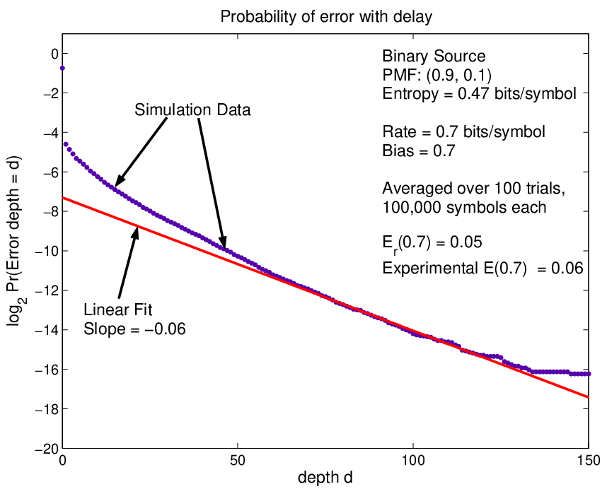
The random time-varying encoder and stack decoder were simulated in software using a random number generator. The ‘experimental’ results are compared with the theory for verification. The probability of error with delay, Pe​(d)P_{e}(d), is the first quantity looked at experimentally. Since probability of error decays exponentially with delay, the logarithm of the probability of error decays linearly with delay. That is,

log2⁡Pe​(d)∼−E⁡(R)​d\log_{2}P_{e}(d)\sim-E(R)d

The slope of the line on a l​o​g2log_{2}-plot is thus the negative of the error exponent achieved by this scheme.

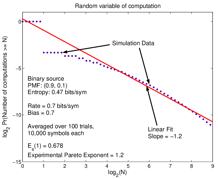
Further, if we assume that the moments of computation at any time are the same as the moments of computation in any incorrect subtree, we can compare the Pareto exponent of the simulation to the theory. This is done by comparing log2⁡P⁡(C≥n)\log_{2}P(C\geq n) versus log2⁡n\log_{2}n on a graph, where CC is the number of computations performed at a time step. The fact that the distribution of computation is asymptotically Paretian should yield that

log2⁡P⁡(C≥n)∼−γ​log2​n\log_{2}P(C\geq n)\sim-\gamma\log_{2}n

where γ\gamma is the Pareto exponent of computation.

IV-A Point to point

Example IV.1

We explore an example of point-to-point lossless source coding that will be comparable to the case when side information is available at the decoder only. The source UiU_{i} is a sequence of IID ℬ⁡(1/2)\mathcal{B}(1/2) random bits. ViV_{i} are generated by passing UiU_{i} through a binary symmetric channel (BSC) with crossover probability ϵ=110\epsilon=\frac{1}{10}. In this example, we consider the case when the side information is available at both the encoder and decoder. The situation is diagrammed in Figure 6. It is clear that since VV is available at both the encoder and decoder, compressing U⊕VU\oplus V is the same as compressing UU. Figure 5 shows the relevant source coding functions for the error random variable U⊕VU\oplus V. Since we are just encoding the noise, the rate must be at least H⁡(U|V)=Hb​(ϵ)H(U|V)=H_{b}(\epsilon) where HbH_{b} is the binary entropy function.

Refer to caption
Fig. 5: Functions of interest associated with a binary source with PMF (0.9,0.1)(0.9,0.1).

We experimentally estimate the error exponent with delay and Pareto exponent of computation. These are shown in Figures 7 and 8 respectively. Again, we see that we can achieve the random coding error exponent and the Pareto exponent guaranteed by theorem 3 holds. Since the bias value (0.7)(0.7) is actually too high to guarantee achieving Er,p​p​(R)E_{r,pp}(R) at rate R=0.7R=0.7, the error exponent in the experiment is somewhat surprising. However, we stress again that the fitting of a line to the curve is somewhat arbitrary and we cannot expect to have precise values of the slope beyond the first digit.

Fig. 6: An example of point-to-point source coding that can be compared to source coding with side information at the decoder. UiU_{i} are Bernoulli (1/2) random bits, VV is UU passed through a BSC with crossover probability ϵ\epsilon. The encoder sequentially bins the error sequence U⊕VU\oplus V.
Theoretical Experimental
Error exponent with delay 0.050.05 ∼0.06\sim 0.06
Pareto exponent of computation ≥1\geq 1 ∼1.2\sim 1.2
Conjectured Pareto exponent 1.2
TABLE II: Comparison of theoretical and experimental performance in example IV.1.
Refer to caption
Fig. 7: Estimating E⁡(R)E(R) for example IV.1.
Refer to caption
Fig. 8: Estimating the Pareto exponent for computation for example IV.1.

IV-B Side information

Fig. 9: An example of lossless source coding with side information at the decoder only. UiU_{i} are Bernoulli (1/2) random bits, VV is UU passed through a BSC with crossover probability ϵ\epsilon. The encoder sequentially bins its observations of UU.
Example IV.2

We reuse the binary source example, where the side information is generated by passing the source bit through a BSC. The side information this time is only available at the decoder, as is shown in Figure 9. In this case, the function Es​i​(ρ)E_{si}(\rho) simplifies66 6 This expansion is for the reviewer’s convenience, it will be removed in the final version. as below,

Es​i​(ρ)\displaystyle E_{si}(\rho) =\displaystyle= OPENlog⁡∑v∈𝒱2⁡(∑u∈𝒰Q​(u,v)1/(1+ρ))1+ρ)\displaystyle\log_{2}\sum_{v\in\mathcal{V}}\Big(\sum_{u\in\mathcal{U}}Q(u,v)^{1/(1+\rho)}\Big)^{1+\rho}\Big) (69)
=\displaystyle= OPENlog⁡∑v∈𝒱2⁡Q⁡(v)​(∑u∈𝒰Q​(u|v)1/(1+ρ))1+ρ)\displaystyle\log_{2}\sum_{v\in\mathcal{V}}Q(v)\Big(\sum_{u\in\mathcal{U}}Q(u|v)^{1/(1+\rho)}\Big)^{1+\rho}\Big) (70)
=\displaystyle= log⁡∑v=012⁡12​(ϵ1/(1+ρ)+(1−ϵ)1/(1+ρ))1+ρ\displaystyle\log_{2}\sum_{v=0}^{1}\frac{1}{2}\Big(\epsilon^{1/(1+\rho)}+(1-\epsilon)^{1/(1+\rho)}\Big)^{1+\rho} (71)
=\displaystyle= (1+ρ)​log2⁡(ϵ1/(1+ρ)+(1−ϵ)1/(1+ρ))\displaystyle(1+\rho)\log_{2}\Big(\epsilon^{1/(1+\rho)}+(1-\epsilon)^{1/(1+\rho)}\Big) (72)

This Es​i​(ρ)E_{si}(\rho) is the same as the Es​(ρ)E_{s}(\rho) function that appears if the side information VV is available at both the encoder and decoder, i.e. point-to-point coding of the error sequence. To compare to the case when VV is available at the encoder as well, we estimate the error exponent with delay and the Pareto exponent for computation through simulation in Figures 10 and 11 respectively. In this simulation, the rate is once again 0.70.7 bits per symbol, and the bias is 0.70.7. We see nearly identical values for the error exponent and Pareto exponent of the two examples, as we should.

Theoretical Experimental
Error exponent with delay 0.050.05 ∼0.08\sim 0.08
Pareto exponent of computation ≥1\geq 1 ∼1.2\sim 1.2
Conjectured Pareto exponent 1.2
TABLE III: Comparison of theoretical and experimental performance in example IV.2.
Refer to caption
Fig. 10: Determining E⁡(R)E(R) for example IV.2.
Refer to caption
Fig. 11: Determining the Pareto exponent for computation for example IV.2.

V Conclusion

In this paper, a scheme was described for the problem of joint source-channel coding with side information available only at the decoder. If the channel is noiseless, one immediately arrives at a scheme for (almost) lossless compression with side information at the decoder only. The coding is done in a ‘streaming’ manner in the sense that source symbols are encoded as they arrive. The encoder consists of an infinite constraint length random time-varying convolutional code, and the decoder is a Stack Algorithm sequential decoder with a variable ‘bias’ parameter.

Two performance measures were bounded for this system when coding IID sources over DMCs; probability of error with end-to-end delay and (average) computational effort of the decoder. We showed that various analogs of Gallager’s random coding error exponent could be achieved by suitable choice of bias. We also bounded the ρt​h\rho^{th} moment of computation for 0≤ρ≤10\leq\rho\leq 1. We thus established a lower bound for the cutoff rate for moments up to the mean for sequential decoding with side information. One would expect that a tweak to the analysis of [28], allowing for side information, would establish the matching upper bounds on the cutoff rate.

Following the work of Koshelev [12], it may be possible to even allow for finite memory Markov sources. Another important extension would be to consider two distributed encoders as in the paper of Slepian and Wolf [1]; the case when the side information VV is coded and required to be reconstructed. The scheme of Section II-B naturally allows for this by adding another tree code for the other source and modifying the metric update slightly. Simulation results have shown that the computation cost seems to be prohibitive except for high rates. Indeed, even the random coding exponents for correlated sources are generally much lower when both sources are coded [31]. Perhaps this is not surprising considering that the computational cutoff rate is closely tied to the ‘Gallager’ EsE_{s} function indirectly through the random coding error exponent.

VI Appendix - Proofs

In this section we prove the theorems of the paper. First we show that the probability of error goes to zero exponentially with delay. This is done initially in the case when there is only a noiseless channel and the source is encoded at some rate RR bits per time unit. Then, we prove this for joint source-channel coding with side information when the source and the channel are ‘synchronized’ at one source symbol per channel use. Next, we prove the theorems regarding the random variable of computation. Again, we do this first in the case of source coding with side information, and then for joint source-channel coding with side information. Before diving into the proofs individually, we first examine the error events that show up.77 7 The appendix is lengthy and somewhat redundant for the convenience of the reviewer and will be trimmed for the final version.

Assume that RR is an integer so we need not worry about integer effects 88 8 For a non-integer rate, the encoder outputs either ⌊R⌋\lfloor R\rfloor or ⌈R⌉\lceil R\rceil bits at every time instant. The integer effect is not important asymptotically, and for convenience we have used the integer assumption in proofs. In simulations, we have used non-integer rates. in the exposition, but the results hold for non-integer rates as well. Similarly, assume in the proof of Theorems 2 and 4 that λ\lambda is an integer.

Fig. 12: Joint source-channel coding with side information available to the decoder.

VI-A Error events

A source produces IID letters (Ui,Vi)(U_{i},V_{i}) according to a joint distribution Q⁡(u,v)Q(u,v) on a discrete alphabet 𝒰×𝒱\mathcal{U}\times\mathcal{V}. The UiU_{i} are available to an encoder, and the ViV_{i} are given to the decoder as side information. In the case of joint source-channel coding, there is a discrete memoryless channel with probability transition matrix W⁡(y|x)W(y|x) with finite input and output alphabets. We use the encoder and decoder of Section II-B. For joint source-channel coding, we assume there is one channel use for every source symbol. We denote vectors as u1d,ynm,…u_{1}^{d},y_{n}^{m},\ldots etc. We reserve the letters uu, xx, and yy for the ‘true’ variables and u~\widetilde{u}, x~\widetilde{x} for arbitrary ‘false’ variables.

The probability measure PP will refer to all randomness in the source as well as the randomly generated encoder. When no confusion arises, QQ will be applied to multiple symbols like u1ku_{1}^{k} with the meaning that Q⁡(u1k)=∏l=1kQ⁡(ul)Q(u_{1}^{k})=\prod_{l=1}^{k}Q(u_{l}).

The stack algorithm uses a metric, (implicity a function of the side information, tree code and channel outputs if there are any), of Γ⁡(u)=log⁡(Q⁡(u|v)​W​(y|x⁡(u))/P⁡(y))+G\Gamma(u)=\log(Q(u|v)W(y|x(u))/P(y))+G for some bias G∈ℝG\in\mathbb{R}, where P⁡(y)=∑xβ⁡(x)​W​(y|x)P(y)=\sum_{x}\beta(x)W(y|x). If there is no channel, Γ⁡(u)=log⁡(Q⁡(u|v))+G\Gamma(u)=\log(Q(u|v))+G if the parities of the sequence match the parities received by the decoder. Otherwise, we can set the metric for non-matching parities to be −∞-\infty to effectively drop them out of the stack. We now consider how the stack decoder could follow a false path. We say the stack decoder ‘visits’ a node if it computes a metric for that node.

Suppose the true source sequence is (u1n,v1n)(u_{1}^{n},v_{1}^{n}) until time nn and u~1n\widetilde{u}_{1}^{n} is some other arbitrary source sequence. Viewed as paths through the encoding tree, u1nu_{1}^{n} and u~1n\widetilde{u}_{1}^{n} are the same if and only if they trace the same path from the root to depth nn in the tree. Also, if they are not the same, there is some earliest point at which they diverge, call that time n−d+1n-d+1. Equivalently, u1n−d=u~1n−du_{1}^{n-d}=\widetilde{u}_{1}^{n-d}, but u1n−d+1≠u~1n−d+1u_{1}^{n-d+1}\neq\widetilde{u}_{1}^{n-d+1}. Until time n−dn-d, because the stack decoder is a sequential decoder, the stack algorithm assigns u1n−du_{1}^{n-d} and u~1n−d\widetilde{u}_{1}^{n-d} the same metric. In order for u~1n\widetilde{u}_{1}^{n} to be the decoder’s estimated path at time nn, a necessary condition is:

Γ⁡(u~1n)≥minn−d+1≤k≤n⁡Γ⁡(u1k)\Gamma(\widetilde{u}_{1}^{n})\geq\min_{n-d+1\leq k\leq n}\Gamma(u_{1}^{k}) (73)

Noting that Γ⁡(u~1n−d)=Γ⁡(u1n−d)\Gamma(\widetilde{u}_{1}^{n-d})=\Gamma(u_{1}^{n-d}), and the fact that the metric is additive, this reduces to:

Γ⁡(u~n−d+1n)≥min1≤k≤d⁡Γ⁡(un−d+1n−d+k)\Gamma(\widetilde{u}_{n-d+1}^{n})\geq\min_{1\leq k\leq d}\Gamma(u_{n-d+1}^{n-d+k}) (74)

All randomness in the source, encoder/decoder, and channel is memoryless and stationary, so the probability of the above event occurring for some false u~n−d+1n\widetilde{u}_{n-d+1}^{n} is the same as the probability of the event FdF_{d} defined below:

Fd≜{∃u~1d∈𝒰d|u~1≠u1,Γ(u~1d)≥min1≤k≤dΓ(u1k)}F_{d}\triangleq\Big\{\exists\widetilde{u}_{1}^{d}\in\mathcal{U}^{d}\Big|\widetilde{u}_{1}\neq u_{1},~\Gamma(\widetilde{u}_{1}^{d})\geq\min_{1\leq k\leq d}\Gamma(u_{1}^{k})\Big\} (75)

We call FdF_{d} the error event of depth dd. Figure 4 shows paths that may lead to an error event of depth 33 occurring, i.e. F3F_{3}. We can further break up FdF_{d} into sub-events Fd,kF_{d,k} so that:

Fd,k\displaystyle F_{d,k} ≜\displaystyle\triangleq {∃u~1d∈𝒰d|u~1≠u1,Γ(u~1d)≥Γ(u1k)}\displaystyle\Big\{\exists\widetilde{u}_{1}^{d}\in\mathcal{U}^{d}\Big|\widetilde{u}_{1}\neq u_{1},~\Gamma(\widetilde{u}_{1}^{d})\geq\Gamma(u_{1}^{k})\Big\} (76)
P⁡(Fd)\displaystyle P(F_{d}) ≤\displaystyle\leq ∑k=1dP⁡(Fd,k)\displaystyle\sum_{k=1}^{d}P(F_{d,k}) (77)
P⁡(Fd,k)\displaystyle P(F_{d,k}) =\displaystyle= E[1(∃u~1d∈𝒰d:u~1≠u1,Γ(u~1d)≥Γ(u1k))]\displaystyle E\Big[1\Big(\exists\widetilde{u}_{1}^{d}\in\mathcal{U}^{d}:\widetilde{u}_{1}\neq u_{1},~\Gamma(\widetilde{u}_{1}^{d})\geq\Gamma(u_{1}^{k})\Big)\Big] (78)
≤\displaystyle\leq E⁡[(∑u~1d∈𝒰d,u~1≠u11​(Γ⁡(u~1d)≥Γ⁡(u1k)))ρ]\displaystyle E\Big[\Big(\sum_{\widetilde{u}_{1}^{d}\in\mathcal{U}^{d},\widetilde{u}_{1}\neq u_{1}}1(\Gamma(\widetilde{u}_{1}^{d})\geq\Gamma(u_{1}^{k}))\Big)^{\rho}\Big] (79)
∀ρ∈[0,1]\displaystyle\forall\rho\in[0,1]

Here 1​(⋅)1(\cdot) denotes the indicator function of its argument. The last line is in fact true for any ρ≥0\rho\geq 0, but it is only useful in bounding if ρ∈[0,1]\rho\in[0,1].

The probability of error with delay dd at time nn is P⁡(u^1n−d​(n)≠u1n−d)P(\widehat{u}_{1}^{n-d}(n)\neq u_{1}^{n-d}), where u^1n−d​(n)\widehat{u}_{1}^{n-d}(n) is the decoder’s estimate of the source from time 11 to n−dn-d produced at time nn. We will give an upper bound on the probability of error independent of nn and depending only on dd, which is an upper bound on Pe​(d)P_{e}(d).

If u^1n−d​(n)≠u1n−d\widehat{u}_{1}^{n-d}(n)\neq u_{1}^{n-d}, then there is some point at which they diverged, say n−d−ln-d-l. So u^1n−d−l​(n)=u1n−d−l\widehat{u}_{1}^{n-d-l}(n)=u_{1}^{n-d-l}, but u^n−d−l+1​(n)≠un−d−l+1\widehat{u}_{n-d-l+1}(n)\neq u_{n-d-l+1}. So the probability that a false decoded path and the true path diverged at time n−d−ln-d-l is at most P⁡(Fd+l)P(F_{d+l}). Now we can use the union bound to get:

P⁡(u^1n−d​(n)≠u1n−d)≤∑l=0n−dP⁡(Fd+l)P(\widehat{u}_{1}^{n-d}(n)\neq u_{1}^{n-d})\leq\sum_{l=0}^{n-d}P(F_{d+l}) (80)

To get a bound independent of nn, we just set nn to infinity and get

Pe​(d)≤∑l=0∞P⁡(Fd+l)P_{e}(d)\leq\sum_{l=0}^{\infty}P(F_{d+l}) (81)

As for the random variable of computation, we define a generic variable NN below 99 9 Sums of the form ∑u1l\sum_{u_{1}^{l}} mean summing over all u1l∈𝒰lu_{1}^{l}\in\mathcal{U}^{l}. This is the meaning for all sums in the appendix, unless an additional condition such as u~1≠u1\widetilde{u}_{1}\neq u_{1} is explicitly stated..

N\displaystyle N ≜\displaystyle\triangleq ∑l=1∞∑u~1l:u~1≠u11(u~1l is visited)\displaystyle\sum_{l=1}^{\infty}\sum_{\widetilde{u}_{1}^{l}:~\widetilde{u}_{1}\neq u_{1}}1\Big(\widetilde{u}_{1}^{l}\textrm{ is visited}\Big) (82)
≤\displaystyle\leq ∑l=1∞∑u~1l:u~1≠u11(Γ(u~1l)≥min1≤k<∞Γ(u1k))\displaystyle\sum_{l=1}^{\infty}\sum_{\widetilde{u}_{1}^{l}:~\widetilde{u}_{1}\neq u_{1}}1\Big(\Gamma(\widetilde{u}_{1}^{l})\geq\min_{1\leq k<\infty}\Gamma(u_{1}^{k})\Big) (83)

By symmetry, it is clear that E⁡[Nγ]=E⁡[Niγ]E[N^{\gamma}]=E[N_{i}^{\gamma}] for all i≥1i\geq 1 and any γ≥0\gamma\geq 0. We want to find when E⁡[Nγ]<∞E[N^{\gamma}]<\infty. By concavity, we have

E⁡[Nγ]\displaystyle E[N^{\gamma}] ≤\displaystyle\leq E[(∑l=1∞∑u~1l:u~1≠u11(Γ(u~1l)≥min1≤k<∞Γ(u1k)))γ]\displaystyle E\Bigg[\bigg(\sum_{l=1}^{\infty}\sum_{\widetilde{u}_{1}^{l}:~\widetilde{u}_{1}\neq u_{1}}1\Big(\Gamma(\widetilde{u}_{1}^{l})\geq\min_{1\leq k<\infty}\Gamma(u_{1}^{k})\bigg)\bigg)^{\gamma}\Bigg] (84)
≤\displaystyle\leq E[(∑l=1∞∑k=1∞∑u~1l:u~1≠u11(Γ(u~1l)≥Γ(u1k)))γ]\displaystyle E\Bigg[\bigg(\sum_{l=1}^{\infty}\sum_{k=1}^{\infty}\sum_{\widetilde{u}_{1}^{l}:~\widetilde{u}_{1}\neq u_{1}}1\Big(\Gamma(\widetilde{u}_{1}^{l})\geq\Gamma(u_{1}^{k})\bigg)\bigg)^{\gamma}\Bigg] (85)
≤\displaystyle\leq ∑l=1∞∑k=1∞E[(∑u~1l:u~1≠u11(Γ(u~1l)≥Γ(u1k)))γ]\displaystyle\sum_{l=1}^{\infty}\sum_{k=1}^{\infty}E\Bigg[\bigg(\sum_{\widetilde{u}_{1}^{l}:~\widetilde{u}_{1}\neq u_{1}}1\Big(\Gamma(\widetilde{u}_{1}^{l})\geq\Gamma(u_{1}^{k})\bigg)\bigg)^{\gamma}\Bigg] (86)
=\displaystyle= ∑l=1∞∑k=1∞Al,k\displaystyle\sum_{l=1}^{\infty}\sum_{k=1}^{\infty}A_{l,k} (87)
Al,k\displaystyle A_{l,k} ≜\displaystyle\triangleq E[(∑u~1l:u~1≠u11(Γ(u~1l)≥Γ(u1k)))γ]\displaystyle E\Bigg[\bigg(\sum_{\widetilde{u}_{1}^{l}:~\widetilde{u}_{1}\neq u_{1}}1\Big(\Gamma(\widetilde{u}_{1}^{l})\geq\Gamma(u_{1}^{k})\bigg)\bigg)^{\gamma}\Bigg] (88)

Here are some further facts/definitions that are repeatedly used in the appendix:

  1. 1.

    The source and channel are memoryless. The parity generation process and channel input generation process are done IID for every branch/node.

  2. 2.

    Jensen’s inequality. If XX is a random variable and ff is a concave ∩\cap function, E⁡[f⁡(X)]≤f⁡(E⁡[X])E[f(X)]\leq f(E[X]). If ρ∈[0,1]\rho\in[0,1], f⁡(x)=xρf(x)=x^{\rho} is concave ∩\cap.

  3. 3.

    By definition, for each y∈𝒴y\in\mathcal{Y}, P⁡(y)=∑x∈𝒳β⁡(x)​W​(y|x)P(y)=\sum_{x\in\mathcal{X}}\beta(x)W(y|x).

  4. 4.

    Definitions of the exponent functions Es​i,E0E_{si},E_{0}, etc. can be found in III-A.

  5. 5.

    Sums and products of probabilities commute, and changing dummy variables can be used to simplify terms. See Gallager [16], Chapter 5.

VI-B Probability of error - source coding with side information

Theorem 5 (Restatement of Theorem 1)

Suppose that the decoder has access to the side information and there is a noiseless rate RR binary channel between the encoder and decoder. Fix any ϵ>0\epsilon>0 and let ρ∈[0,1]\rho\in[0,1]. For the encoder/decoder of Section II-B, if the bias GG satisfies

G≤1+ρρ​[Es​i​(ρ)−Fs​i​(ρ)]G\leq\frac{1+\rho}{\rho}\bigg[E_{si}(\rho)-F_{si}(\rho)\bigg] (89)

then, there is a constant Kϵ<∞K_{\epsilon}<\infty so that

Pe​(d)<Kϵ​exp2⁡(−d⁡(ρ​R−Es​i​(ρ)−ϵ))P_{e}(d)<K_{\epsilon}\exp_{2}\bigg(-d\Big(\rho R-E_{si}(\rho)-\epsilon\Big)\bigg) (90)

Hence, with suitable choice of bias, the error exponent with delay can be

E⁡(R)=Er,s​i​(R)≜supρ∈[0,1]ρ​R−Es​i​(ρ)E(R)=E_{r,si}(R)\triangleq\sup_{\rho\in[0,1]}\rho R-E_{si}(\rho) (91)
Proof:

The letter BB will be used for the bits received by the decoder, which will be referred to as ‘parities’. We can specialize the event FdF_{d} to this situation and write it as:

Fd≜{∃u~1d,u~1≠u1|Γ(u~1d)≥min1≤k≤dΓ(u1k) and parities of u~1d match B1d​R}F_{d}\triangleq\Big\{\exists\ \widetilde{u}_{1}^{d}\ ,\ \widetilde{u}_{1}\neq u_{1}\ \Big|\ \Gamma(\widetilde{u}_{1}^{d})\geq\min_{1\leq k\leq d}\Gamma(u_{1}^{k})\textrm{ and parities of $\widetilde{u}_{1}^{d}$ match $B_{1}^{dR}$}\Big\} (92)

The event FdF_{d} can be subdivided into events Fd,kF_{d,k} so that Fd=⋃k=1dFd,kF_{d}=\bigcup_{k=1}^{d}F_{d,k}, where

Fd,k≜{∃u~1d,u~1≠u1|Γ(u~1d)≥Γ(u1k) and parities of u~1d match B1d​R}F_{d,k}\triangleq\Big\{\exists\ \widetilde{u}_{1}^{d}\ ,\widetilde{u}_{1}\neq u_{1}\Big|\quad\Gamma(\widetilde{u}_{1}^{d})\geq\Gamma(u_{1}^{k})\textrm{ and parities of $\widetilde{u}_{1}^{d}$ match $B_{1}^{dR}$}\Big\} (93)

Suppose u~1d\widetilde{u}_{1}^{d} is a false path that causes Fd,kF_{d,k} to occur. This means its parities match the received bits and its metric Γ⁡(u~1d)\Gamma(\widetilde{u}_{1}^{d}) is at least Γ⁡(u1k)\Gamma(u_{1}^{k}). Therefore,

0\displaystyle 0 ≤\displaystyle\leq Γ⁡(u~1d)−Γ⁡(u1k)\displaystyle\Gamma(\widetilde{u}_{1}^{d})-\Gamma(u_{1}^{k}) (94)
=\displaystyle= ∑l=1d(log⁡(Q⁡(u~l|vl))+G)−∑l=1k(log⁡(Q⁡(ul|vl))+G)\displaystyle\sum_{l=1}^{d}\Big(\log(Q(\widetilde{u}_{l}|v_{l}))+G\Big)-\sum_{l=1}^{k}\Big(\log(Q(u_{l}|v_{l}))+G\Big) (95)
=\displaystyle= ∑l=1klog⁡(Q⁡(u~l|vl)Q⁡(ul|vl))+∑l=k+1dlog⁡Q⁡(u~l|vl)+(d−k)​G\displaystyle\sum_{l=1}^{k}\log\Big(\frac{Q(\widetilde{u}_{l}|v_{l})}{Q(u_{l}|v_{l})}\Big)+\sum_{l=k+1}^{d}\log Q(\widetilde{u}_{l}|v_{l})+(d-k)G (96)

Using a Gallager-style union bound, for ρ∈[0,1]\rho\in[0,1], we have

P⁡(Fd,k)\displaystyle P(F_{d,k}) ≤\displaystyle\leq E[(∑u~1d:u~1≠x11(u~1d causes Fd,k to occur))ρ]\displaystyle E\bigg[\Big(\sum_{\widetilde{u}_{1}^{d}:\ \widetilde{u}_{1}\neq x_{1}}1(\textrm{$\widetilde{u}_{1}^{d}$ causes $F_{d,k}$ to occur})\Big)^{\rho}\bigg] (97)
≤(a)\displaystyle\stackrel{{\scriptstyle(a)}}{{\leq}} (∑u~1d,u~1≠x1E⁡[1​(u~1d causes Fd,k to occur)])ρ\displaystyle\bigg(\sum_{\widetilde{u}_{1}^{d},\ \widetilde{u}_{1}\neq x_{1}}E\Big[1(\textrm{$\widetilde{u}_{1}^{d}$ causes $F_{d,k}$ to occur})\Big]\bigg)^{\rho} (98)

Here, (a) is by Jensen’s inequality. By conditioning on the source sequence and applying the union bound, we get

P⁡(Fd)\displaystyle P(F_{d}) =\displaystyle= ∑u1d∈𝒰d,v1d∈𝒱dQ⁡(u1d,v1d)​P​(Fd|u1d,v1d)\displaystyle\sum_{u_{1}^{d}\in\mathcal{U}^{d},v_{1}^{d}\in\mathcal{V}^{d}}Q(u_{1}^{d},v_{1}^{d})P(F_{d}|u_{1}^{d},v_{1}^{d}) (99)
≤\displaystyle\leq ∑u1d,v1dQ⁡(u1d,v1d)​∑k=1dP⁡(Fd,k|u1d,v1d)\displaystyle\sum_{u_{1}^{d},v_{1}^{d}}Q(u_{1}^{d},v_{1}^{d})\sum_{k=1}^{d}P(F_{d,k}|u_{1}^{d},v_{1}^{d}) (100)
=\displaystyle= ∑k=1d∑u1d,v1dQ⁡(u1d,v1d)​P​(Fd,k|u1d,v1d)\displaystyle\sum_{k=1}^{d}\sum_{u_{1}^{d},v_{1}^{d}}Q(u_{1}^{d},v_{1}^{d})P(F_{d,k}|u_{1}^{d},v_{1}^{d}) (101)
≤\displaystyle\leq ∑k=1d∑u1d,v1dQ(u1d,v1d)(∑u~1d,u~1≠x1E[1(u~1d causes Fd,k to occur)|u1d,v1d])ρ\displaystyle\sum_{k=1}^{d}\sum_{u_{1}^{d},v_{1}^{d}}Q(u_{1}^{d},v_{1}^{d})\bigg(\sum_{\widetilde{u}_{1}^{d},\ \widetilde{u}_{1}\neq x_{1}}E\Big[1(\textrm{$\widetilde{u}_{1}^{d}$ causes $F_{d,k}$ to occur})\Big|u_{1}^{d},v_{1}^{d}\Big]\bigg)^{\rho} (102)
≜\displaystyle\triangleq ∑k=1d∑u1d,v1dQ⁡(u1d,v1d)​(∑u~1d,u~1≠x1Ak​(u~1d,u1d,v1d))ρ\displaystyle\sum_{k=1}^{d}\sum_{u_{1}^{d},v_{1}^{d}}Q(u_{1}^{d},v_{1}^{d})\bigg(\sum_{\widetilde{u}_{1}^{d},\ \widetilde{u}_{1}\neq x_{1}}A_{k}(\widetilde{u}_{1}^{d},u_{1}^{d},v_{1}^{d})\bigg)^{\rho} (103)

Continuing with the bounding, we use the fact that the parity generation process is independent1010 10 Only pairwise independence of the parities along two disjoint paths is required. of everything else to get

Ak​(u~1d,u1d,v1d)\displaystyle A_{k}(\widetilde{u}_{1}^{d},u_{1}^{d},v_{1}^{d}) =\displaystyle= E[1(parities of u~1d match B1d​R)⋅1(Γ(u~1d)≥Γ(u1k))|u1d,v1d]\displaystyle E\Big[1(\textrm{parities of $\widetilde{u}_{1}^{d}$ match $B_{1}^{dR}$})\cdot 1(\Gamma(\widetilde{u}_{1}^{d})\geq\Gamma(u_{1}^{k}))\Big|u_{1}^{d},v_{1}^{d}\Big] (104)
=\displaystyle= E[1(parities of u~1d match B1d​R)]E[1(Γ(u~1d)≥Γ(u1k))|u1d,v1d]\displaystyle E\Big[1(\textrm{parities of $\widetilde{u}_{1}^{d}$ match $B_{1}^{dR}$})\Big]E\Big[1(\Gamma(\widetilde{u}_{1}^{d})\geq\Gamma(u_{1}^{k}))\Big|u_{1}^{d},v_{1}^{d}\Big] (105)
=\displaystyle= 2−d​RE[1(Γ(u~1d)≥Γ(u1k))|u1d,v1d]\displaystyle 2^{-dR}E\Big[1(\Gamma(\widetilde{u}_{1}^{d})\geq\Gamma(u_{1}^{k}))\Big|u_{1}^{d},v_{1}^{d}\Big] (106)
≤\displaystyle\leq exp2⁡(−d​R)⋅exp2⁡(s⁡(Γ⁡(u~1d)−Γ⁡(u1k)))\displaystyle\exp_{2}(-dR)\cdot\exp_{2}\Big(s(\Gamma(\widetilde{u}_{1}^{d})-\Gamma(u_{1}^{k}))\Big) (107)
=\displaystyle= exp2⁡(−d​R)⋅exp2⁡(s⁡[log2⁡Q⁡(u~1k|v1k)Q⁡(u1k|v1k)+log2⁡Q⁡(u~k+1d|vk+1d)+(d−k)​G])\displaystyle\exp_{2}(-dR)\cdot\exp_{2}\Big(s\Big[\log_{2}\frac{Q(\widetilde{u}_{1}^{k}|v_{1}^{k})}{Q(u_{1}^{k}|v_{1}^{k})}+\log_{2}Q(\widetilde{u}_{k+1}^{d}|v_{k+1}^{d})+(d-k)G\Big]\Big) (108)
for any s≥0s\geq 0

Substituting for Ak​(u~1d,u1d,v1d)A_{k}(\widetilde{u}_{1}^{d},u_{1}^{d},v_{1}^{d}), and removing the restriction that u~1≠u1\widetilde{u}_{1}\neq u_{1},

P⁡(Fd,k|u1d,v1d)\displaystyle P(F_{d,k}|u_{1}^{d},v_{1}^{d}) ≤\displaystyle\leq (∑u~1dexp2⁡(−d​R)​exp2⁡(s⁡[log2⁡Q⁡(u~1k|v1k)Q⁡(u1k|v1k)+log2⁡Q⁡(u~k+1d|vk+1d)+(d−k)​G]))ρ\displaystyle\bigg(\sum_{\widetilde{u}_{1}^{d}}\exp_{2}(-dR)\exp_{2}\Big(s\Big[\log_{2}\frac{Q(\widetilde{u}_{1}^{k}|v_{1}^{k})}{Q(u_{1}^{k}|v_{1}^{k})}+\log_{2}Q(\widetilde{u}_{k+1}^{d}|v_{k+1}^{d})+(d-k)G\Big]\Big)\bigg)^{\rho} (109)
=\displaystyle= exp2⁡(−d​ρ​R+(d−k)​s​ρ​G)​(∑u~1d(Q⁡(u~1k|v1k)Q⁡(u1k|v1k))s​Q​(u~k+1d|vk+1d)s)ρ\displaystyle\exp_{2}(-d\rho R+(d-k)s\rho G)\bigg(\sum_{\widetilde{u}_{1}^{d}}\Big(\frac{Q(\widetilde{u}_{1}^{k}|v_{1}^{k})}{Q(u_{1}^{k}|v_{1}^{k})}\Big)^{s}Q(\widetilde{u}_{k+1}^{d}|v_{k+1}^{d})^{s}\bigg)^{\rho} (110)
=(b)\displaystyle\stackrel{{\scriptstyle(b)}}{{=}} exp2⁡(−d​ρ​R+(d−k)​s​ρ​G)​(∑u~1k(Q⁡(u~1k|v1k)Q⁡(u1k|v1k))s)ρ​(∑u~k+1dQ​(u~k+1d|vk+1d)s)ρ\displaystyle\exp_{2}(-d\rho R+(d-k)s\rho G)\bigg(\sum_{\widetilde{u}_{1}^{k}}\Big(\frac{Q(\widetilde{u}_{1}^{k}|v_{1}^{k})}{Q(u_{1}^{k}|v_{1}^{k})}\Big)^{s}\bigg)^{\rho}\bigg(\sum_{\widetilde{u}_{k+1}^{d}}Q(\widetilde{u}_{k+1}^{d}|v_{k+1}^{d})^{s}\bigg)^{\rho} (111)

Relation (b) follows from the standard algebra of interchanging sums and products. Now, we substitute the last line into (103).

P⁡(Fd)\displaystyle P(F_{d}) ≤\displaystyle\leq ∑k=1d2−d​ρ​R+(d−k)​s​ρ​G∑v1dQ(v1d)∑u1k∑uk+1dQ(u1k|v1k)Q(uk+1d|vk+1d)⋅\displaystyle\sum_{k=1}^{d}2^{-d\rho R+(d-k)s\rho G}\sum_{v_{1}^{d}}Q(v_{1}^{d})\sum_{u_{1}^{k}}\sum_{u_{k+1}^{d}}Q(u_{1}^{k}|v_{1}^{k})Q(u_{k+1}^{d}|v_{k+1}^{d})\cdot (115)
(∑u~1k(Q⁡(u~1k|v1k)Q⁡(u1k|v1k))s)ρ​(∑u~k+1dQ​(u~k+1d|vk+1d)s)ρ\displaystyle\hskip 42.67912pt\Big(\sum_{\widetilde{u}_{1}^{k}}\Big(\frac{Q(\widetilde{u}_{1}^{k}|v_{1}^{k})}{Q(u_{1}^{k}|v_{1}^{k})}\Big)^{s}\Big)^{\rho}\Big(\sum_{\widetilde{u}_{k+1}^{d}}Q(\widetilde{u}_{k+1}^{d}|v_{k+1}^{d})^{s}\Big)^{\rho}
=\displaystyle= ∑k=1d2−d​ρ​R+(d−k)​s​ρ​G​∑v1kQ⁡(v1k)​∑vk+1dQ⁡(vk+1d)​∑u1kQ​(u1k|v1k)1−s​ρ\displaystyle\sum_{k=1}^{d}2^{-d\rho R+(d-k)s\rho G}\sum_{v_{1}^{k}}Q(v_{1}^{k})\sum_{v_{k+1}^{d}}Q(v_{k+1}^{d})\sum_{u_{1}^{k}}Q(u_{1}^{k}|v_{1}^{k})^{1-s\rho}
(∑u~1kQ​(u~1k|v1k)s)ρ​∑uk+1dQ⁡(uk+1d|vk+1d)​(∑u~k+1dQ​(u~k+1d|vk+1d)s)ρ\displaystyle\hskip 42.67912pt\Big(\sum_{\widetilde{u}_{1}^{k}}Q(\widetilde{u}_{1}^{k}|v_{1}^{k})^{s}\Big)^{\rho}\sum_{u_{k+1}^{d}}Q(u_{k+1}^{d}|v_{k+1}^{d})\Big(\sum_{\widetilde{u}_{k+1}^{d}}Q(\widetilde{u}_{k+1}^{d}|v_{k+1}^{d})^{s}\Big)^{\rho}
=\displaystyle= ∑k=1d2−d​ρ​R+(d−k)​s​ρ​G∑v1kQ(v1k)∑vk+1dQ(vk+1d)(∑u1kQ(u1k|v1k)1−s​ρ)⋅\displaystyle\sum_{k=1}^{d}2^{-d\rho R+(d-k)s\rho G}\sum_{v_{1}^{k}}Q(v_{1}^{k})\sum_{v_{k+1}^{d}}Q(v_{k+1}^{d})\Big(\sum_{u_{1}^{k}}Q(u_{1}^{k}|v_{1}^{k})^{1-s\rho}\Big)\cdot
(∑u~1kQ​(u~1k|v1k)s)ρ​(∑u~k+1dQ​(u~k+1d|vk+1d)s)ρ\displaystyle\hskip 42.67912pt\Big(\sum_{\widetilde{u}_{1}^{k}}Q(\widetilde{u}_{1}^{k}|v_{1}^{k})^{s}\Big)^{\rho}\Big(\sum_{\widetilde{u}_{k+1}^{d}}Q(\widetilde{u}_{k+1}^{d}|v_{k+1}^{d})^{s}\Big)^{\rho}
=(c)\displaystyle\stackrel{{\scriptstyle(c)}}{{=}} ∑k=1d2−d​ρ​R+(d−k)​ρ1+ρ​G∑v1kQ(v1k)(∑u1kQ(u1k|v1k)11+ρ)1+ρ⋅\displaystyle\sum_{k=1}^{d}2^{-d\rho R+(d-k)\frac{\rho}{1+\rho}G}\sum_{v_{1}^{k}}Q(v_{1}^{k})\Big(\sum_{u_{1}^{k}}Q(u_{1}^{k}|v_{1}^{k})^{\frac{1}{1+\rho}}\Big)^{1+\rho}\cdot
∑vk+1dQ⁡(vk+1d)​(∑uk+1dQ​(uk+1d|vk+1d)11+ρ)ρ\displaystyle\hskip 42.67912pt\sum_{v_{k+1}^{d}}Q(v_{k+1}^{d})\Big(\sum_{u_{k+1}^{d}}Q(u_{k+1}^{d}|v_{k+1}^{d})^{\frac{1}{1+\rho}}\Big)^{\rho}

We get (c) by noting that the u~\widetilde{u}’s are just dummy variables and we are free to replace them with uu’s and then setting s=11+ρs=\frac{1}{1+\rho}. Next, we use the IID property of the source along with some algebra to get to an exponential form. For example, we have

∑v1kQ⁡(v1k)​(∑u1kQ​(u1k|v1k)11+ρ)1+ρ\displaystyle\sum_{v_{1}^{k}}Q(v_{1}^{k})\Big(\sum_{u_{1}^{k}}Q(u_{1}^{k}|v_{1}^{k})^{\frac{1}{1+\rho}}\Big)^{1+\rho} =\displaystyle= ∑v1⋯∑vk∏l=1kQ(vl)(∑u1∑u2⋯∑uk∏l=1kQ(ul|vl)11+ρ)1+ρ\displaystyle\sum_{v_{1}}\cdots\sum_{v_{k}}\prod_{l=1}^{k}Q(v_{l})\Big(\sum_{u_{1}}\sum_{u_{2}}\cdots\sum_{u_{k}}\prod_{l=1}^{k}Q(u_{l}|v_{l})^{\frac{1}{1+\rho}}\Big)^{1+\rho} (116)
=\displaystyle= ∏l=1k∑vlQ⁡(vl)​(∑ulQ​(ul|vl)11+ρ)1+ρ\displaystyle\prod_{l=1}^{k}\sum_{v_{l}}Q(v_{l})\Big(\sum_{u_{l}}Q(u_{l}|v_{l})^{\frac{1}{1+\rho}}\Big)^{1+\rho} (117)
=\displaystyle= [∑v∈𝒱(∑u∈𝒰Q​(u,v)11+ρ)1+ρ]k\displaystyle\bigg[\sum_{v\in\mathcal{V}}\Big(\sum_{u\in\mathcal{U}}Q(u,v)^{\frac{1}{1+\rho}}\Big)^{1+\rho}\bigg]^{k} (118)

Similarly,

∑v1kQ⁡(v1k)​(∑u1kQ​(u1k|v1k)11+ρ)ρ\displaystyle\sum_{v_{1}^{k}}Q(v_{1}^{k})\Big(\sum_{u_{1}^{k}}Q(u_{1}^{k}|v_{1}^{k})^{\frac{1}{1+\rho}}\Big)^{\rho} =\displaystyle= ∑v1⋯∑vk∏l=1kQ(vl)(∑u1∑u2⋯∑uk∏l=1kQ(ul|vl)11+ρ)ρ\displaystyle\sum_{v_{1}}\cdots\sum_{v_{k}}\prod_{l=1}^{k}Q(v_{l})\Big(\sum_{u_{1}}\sum_{u_{2}}\cdots\sum_{u_{k}}\prod_{l=1}^{k}Q(u_{l}|v_{l})^{\frac{1}{1+\rho}}\Big)^{\rho} (119)
=\displaystyle= ∏l=1k∑vlQ⁡(vl)​(∑ulQ​(ul|vl)11+ρ)ρ\displaystyle\prod_{l=1}^{k}\sum_{v_{l}}Q(v_{l})\Big(\sum_{u_{l}}Q(u_{l}|v_{l})^{\frac{1}{1+\rho}}\Big)^{\rho} (120)
=\displaystyle= [∑v∈𝒱Q⁡(v)​(∑u∈𝒰Q​(u|v)11+ρ)ρ]k\displaystyle\bigg[\sum_{v\in\mathcal{V}}Q(v)\Big(\sum_{u\in\mathcal{U}}Q(u|v)^{\frac{1}{1+\rho}}\Big)^{\rho}\bigg]^{k} (121)

Using the definitions of Es​i​(ρ)E_{si}(\rho) and Fs​i​(ρ)F_{si}(\rho), we can rewrite the bound as:

P⁡(Fd)\displaystyle P(F_{d}) ≤\displaystyle\leq ∑k=1dexp⁡(−d​ρ​R+(d−k)​ρ1+ρ​G+k​Es​i​(ρ)+(d−k)​Fs​i​(ρ))\displaystyle\sum_{k=1}^{d}\exp\Big(-d\rho R+(d-k)\frac{\rho}{1+\rho}G+kE_{si}(\rho)+(d-k)F_{si}(\rho)\Big) (122)
=\displaystyle= exp⁡(d⁡(ρ1+ρ​G+Fs​i​(ρ)−ρ​R))​∑k=1dexp⁡(k⁡(Es​i​(ρ)−Fs​i​(ρ)−ρ1+ρ​G)CLOSE\displaystyle\exp\Big(d\big(\frac{\rho}{1+\rho}G+F_{si}(\rho)-\rho R\big)\Big)\sum_{k=1}^{d}\exp\Big(k\big(E_{si}(\rho)-F_{si}(\rho)-\frac{\rho}{1+\rho}G\big) (123)

By the assumption of the theorem, (89), the following condition holds

Es​i​(ρ)−Fs​i​(ρ)−ρ1+ρ​G≥0E_{si}(\rho)-F_{si}(\rho)-\frac{\rho}{1+\rho}G\geq 0 (124)

Then, we can simplify the bound to

P⁡(Fd)\displaystyle P(F_{d}) ≤\displaystyle\leq exp⁡(d⁡(ρ1+ρ​G+Fs​i​(ρ)−ρ​R))​∑k=1dexp⁡(k⁡(Es​i​(ρ)−Fs​i​(ρ)−ρ1+ρ​G))\displaystyle\exp\Big(d\big(\frac{\rho}{1+\rho}G+F_{si}(\rho)-\rho R\big)\Big)\sum_{k=1}^{d}\exp\Big(k\big(E_{si}(\rho)-F_{si}(\rho)-\frac{\rho}{1+\rho}G\big)\Big) (125)
≤(d)\displaystyle\stackrel{{\scriptstyle(d)}}{{\leq}} exp⁡(d⁡(ρ1+ρ​G+Fs​i​(ρ)−ρ​R))⋅d​exp⁡(d⁡(Es​i​(ρ)−Fs​i​(ρ)−ρ1+ρ​G))\displaystyle\exp\Big(d\big(\frac{\rho}{1+\rho}G+F_{si}(\rho)-\rho R\big)\Big)\cdot d\exp\Big(d\big(E_{si}(\rho)-F_{si}(\rho)-\frac{\rho}{1+\rho}G\big)\Big) (126)
=\displaystyle= d​exp⁡(−d⁡(ρ​R−Es​i​(ρ)))\displaystyle d\exp\Big(-d(\rho R-E_{si}(\rho))\Big) (127)

We get (d) from noting that the sum of the geometric series can be upper bounded by dd times the largest term. Now this holds for all ρ∈[0,1]\rho\in[0,1], so

P⁡(Fd)\displaystyle P(F_{d}) ≤\displaystyle\leq Kϵ​exp⁡(−d⁡(ρ​R−Es​i​(ρ)−ϵ))\displaystyle K_{\epsilon}\exp\Big(-d(\rho R-E_{si}(\rho)-\epsilon)\Big) (128)
K~ϵ\displaystyle\widetilde{K}_{\epsilon} ≜\displaystyle\triangleq max⁡{d:log⁡dd≥ϵ}<∞\displaystyle\max\Big\{d:\frac{\log d}{d}\geq\epsilon\Big\}<\infty (129)

Note that K~ϵ<∞\widetilde{K}_{\epsilon}<\infty and is independent of dd because ln⁡(d)/d\ln(d)/d goes to 00. We note that Es​i​(ρ)E_{si}(\rho) is a differentiable function for all ρ≥0\rho\geq 0, with Es​i′​(0)=H⁡(U|V)E_{si}^{\prime}(0)=H(U|V) (see [18]); that is, the slope at 00 is the conditional entropy of the source UU given the side information VV. Es​i​(ρ)E_{si}(\rho) is the source coding with side information coding analog to Gallager’s function E0​(ρ)E_{0}(\rho). While Gallager’s function may be non-differentiable at points because it is the maximization of a function over probability distributions, Es​i​(ρ)E_{si}(\rho) doesn’t suffer from this problem.

Now, assuming the bias satisfies the required condition, we have

Pe​(d)\displaystyle P_{e}(d) ≤\displaystyle\leq ∑k=0∞P⁡(Fd+k)\displaystyle\sum_{k=0}^{\infty}P(F_{d+k}) (130)
≤\displaystyle\leq ∑k=0∞K~ϵ​2−(d+k)​(ρ​R−Es​i​(ρ)−ϵ)\displaystyle\sum_{k=0}^{\infty}\widetilde{K}_{\epsilon}2^{-(d+k)(\rho R-E_{si}(\rho)-\epsilon)} (131)
=\displaystyle= exp⁡(−d⁡(ρ​R−Es​i​(ρ)−ϵ))​∑k=0∞K~ϵ​2−k⁡(ρ​R−Es​i​(ρ)−ϵ)\displaystyle\exp\Big(-d(\rho R-E_{si}(\rho)-\epsilon)\Big)\sum_{k=0}^{\infty}\widetilde{K}_{\epsilon}2^{-k(\rho R-E_{si}(\rho)-\epsilon)} (132)

Since we can choose ϵ\epsilon arbitrarily small, the geometric series converges and we have

Pe​(d)\displaystyle P_{e}(d) ≤\displaystyle\leq K~ϵ1−2−(ρ​R−Es​i​(ρ)−ϵ)​2−d⁡(ρ​R−Es​i​(ρ)−ϵ)\displaystyle\frac{\widetilde{K}_{\epsilon}}{1-2^{-(\rho R-E_{si}(\rho)-\epsilon)}}2^{-d(\rho R-E_{si}(\rho)-\epsilon)} (133)
=\displaystyle= K~ϵ​exp2⁡(−d⁡(ρ​R−Es​i​(ρ)−ϵ))\displaystyle\tilde{K}_{\epsilon}\exp_{2}\Big(-d(\rho R-E_{si}(\rho)-\epsilon)\Big) (134)

This is true for all ρ∈[0,1]\rho\in[0,1], so E⁡(R)≥Er,s​i​(R)=supρ∈[0,1]ρ​R−Es​i​(ρ)E(R)\geq E_{r,si}(R)=\sup_{\rho\in[0,1]}\rho R-E_{si}(\rho). ∎

VI-C Probability of error - joint source channel coding with side information

Theorem 6 (Restatement of Theorem 2)

Suppose there is a channel WW between the encoder and the decoder and side information is available to the decoder. Fix any ϵ>0\epsilon>0 and let ρ∈[0,1]\rho\in[0,1]. For the encoder/decoder of Sections II-B and II-C, if the bias GG satisfies

G≤1+ρρ​[Es​i​(ρ)−Fs​i​(ρ)−λ​E0​(ρ)+λ​F​(ρ)]G\leq\frac{1+\rho}{\rho}\bigg[E_{si}(\rho)-F_{si}(\rho)-\lambda E_{0}(\rho)+\lambda F(\rho)\bigg] (135)

then, there is a constant Kϵ<∞K_{\epsilon}<\infty so that

Pe​(d)<Kϵ​exp2⁡(−d⁡(λ​E0​(ρ)−Es​i​(ρ)−ϵ))P_{e}(d)<K_{\epsilon}\exp_{2}\bigg(-d\Big(\lambda E_{0}(\rho)-E_{si}(\rho)-\epsilon\Big)\bigg) (136)

Hence, with suitable choice of bias, the error exponent with delay can be

E⁡(λ)=Er,j​s​c​s​i​(λ)≜supρ∈[0,1]λ​E0​(ρ)−Es​i​(ρ)E(\lambda)=E_{r,jscsi}(\lambda)\triangleq\sup_{\rho\in[0,1]}\lambda E_{0}(\rho)-E_{si}(\rho) (137)
Proof:

We will prove this for λ=1\lambda=1 and then show how the proof changes for other λ\lambda. As in the previous proof, Pe​(d)P_{e}(d) can be bounded by ∑l=0∞P⁡(Fd+l)\sum_{l=0}^{\infty}P(F_{d+l}), and P⁡(Fd)P(F_{d}) can be bounded by ∑k=1dP⁡(Fd,k)\sum_{k=1}^{d}P(F_{d,k}). So we start by bounding P⁡(Fd,k)P(F_{d,k}). First condition on the true source sequence, channel inputs and channel outputs.

P⁡(Fd,k)\displaystyle P(F_{d,k}) ≤\displaystyle\leq ∑u1d,v1d,x1d,y1dQ(u1d,v1d)R(x1d)W(y1d|x1d)E[(∑u~1d∈𝒰d,u~1≠u11(Γ(u~1d)≥Γ(u1k)))ρ|x1d,y1d,u1d,v1d]\displaystyle\sum_{u_{1}^{d},v_{1}^{d},x_{1}^{d},y_{1}^{d}}Q(u_{1}^{d},v_{1}^{d})R(x_{1}^{d})W(y_{1}^{d}|x_{1}^{d})E\Big[\Big(\sum_{\widetilde{u}_{1}^{d}\in\mathcal{U}^{d},\widetilde{u}_{1}\neq u_{1}}1(\Gamma(\widetilde{u}_{1}^{d})\geq\Gamma(u_{1}^{k}))\Big)^{\rho}\Big|x_{1}^{d},y_{1}^{d},u_{1}^{d},v_{1}^{d}\Big] (138)
≤\displaystyle\leq ∑u1d,v1d,x1d,y1dQ(u1d,v1d)R(x1d)W(y1d|x1d)(E[∑u~1d∈𝒰d,u~1≠u11(Γ(u~1d)≥Γ(u1k))|x1d,y1d,u1d,v1d])ρ\displaystyle\sum_{u_{1}^{d},v_{1}^{d},x_{1}^{d},y_{1}^{d}}Q(u_{1}^{d},v_{1}^{d})R(x_{1}^{d})W(y_{1}^{d}|x_{1}^{d})\bigg(E\Big[\sum_{\widetilde{u}_{1}^{d}\in\mathcal{U}^{d},\widetilde{u}_{1}\neq u_{1}}1(\Gamma(\widetilde{u}_{1}^{d})\geq\Gamma(u_{1}^{k}))\Big|x_{1}^{d},y_{1}^{d},u_{1}^{d},v_{1}^{d}\Big]\bigg)^{\rho} (139)

The last step is true by Jensen’s inequality. Now the only thing that is random in the expectation is the channel symbols used on the false u~\widetilde{u} paths.

P⁡(Fd,k)\displaystyle P(F_{d,k}) ≤\displaystyle\leq ∑u1d,v1d,x1d,y1dQ(u1d,v1d)R(x1d)W(y1d|x1d)⋅\displaystyle\sum_{u_{1}^{d},v_{1}^{d},x_{1}^{d},~y_{1}^{d}}Q(u_{1}^{d},v_{1}^{d})R(x_{1}^{d})W(y_{1}^{d}|x_{1}^{d})\cdot (141)
⋅(∑u~1d∈𝒰d,u~1≠u1∑x~1dR(x~1d)E[1(Γ(u~1d)≥Γ(u1k))|x1d,y1d,u1d,v1d,x~1d])ρ\displaystyle\hskip 56.9055pt\cdot\bigg(\sum_{\widetilde{u}_{1}^{d}\in\mathcal{U}^{d},~\widetilde{u}_{1}\neq u_{1}}\sum_{\widetilde{x}_{1}^{d}}R(\widetilde{x}_{1}^{d})E\Big[1(\Gamma(\widetilde{u}_{1}^{d})\geq\Gamma(u_{1}^{k}))\Big|x_{1}^{d},y_{1}^{d},u_{1}^{d},v_{1}^{d},\widetilde{x}_{1}^{d}\Big]\bigg)^{\rho}

Now, we also have for all s≥0s\geq 0, 1​(Γ⁡(u~1d)≥Γ⁡(u1k))≤exp2⁡(s⁡(Γ⁡(u~1d)−Γ⁡(u1k)))1(\Gamma(\widetilde{u}_{1}^{d})\geq\Gamma(u_{1}^{k}))\leq\exp_{2}(s(\Gamma(\widetilde{u}_{1}^{d})-\Gamma(u_{1}^{k}))). So,

Γ⁡(u~1d)−Γ⁡(u1k)\displaystyle\Gamma(\widetilde{u}_{1}^{d})-\Gamma(u_{1}^{k}) =\displaystyle= log2⁡Q⁡(u~1d|v1d)​W​(y1d|x~1d)P⁡(y1d)−log2⁡Q⁡(u1k|v1k)​W​(y1k|x1k)P⁡(y1k)+(d−k)​G\displaystyle\log_{2}\frac{Q(\widetilde{u}_{1}^{d}|v_{1}^{d})W(y_{1}^{d}|\widetilde{x}_{1}^{d})}{P(y_{1}^{d})}-\log_{2}\frac{Q(u_{1}^{k}|v_{1}^{k})W(y_{1}^{k}|x_{1}^{k})}{P(y_{1}^{k})}+(d-k)G (142)
1​(Γ⁡(u~1d)≥Γ⁡(u1k))\displaystyle 1(\Gamma(\widetilde{u}_{1}^{d})\geq\Gamma(u_{1}^{k})) ≤\displaystyle\leq (Q⁡(u~1k|v1k)​W​(y1k|x~1k)​W​(yk+1d|x~k+1d)​Q​(u~k+1d|vk+1d)Q⁡(u1k|v1k)​W​(y1k|x1k)​P​(yk+1d))s​2s⁡(d−k)​G\displaystyle\Bigg(\frac{Q(\widetilde{u}_{1}^{k}|v_{1}^{k})W(y_{1}^{k}|\widetilde{x}_{1}^{k})W(y_{k+1}^{d}|\widetilde{x}_{k+1}^{d})Q(\widetilde{u}_{k+1}^{d}|v_{k+1}^{d})}{Q(u_{1}^{k}|v_{1}^{k})W(y_{1}^{k}|x_{1}^{k})P(y_{k+1}^{d})}\Bigg)^{s}2^{s(d-k)G} (143)

We can substitute this expression into the inequality for P⁡(Fd,k)P(F_{d,k}).

P⁡(Fd,k)\displaystyle P(F_{d,k}) ≤\displaystyle\leq ∑u1d,v1d,x1d,y1dQ(v1d)Q(u1k|v1k)1−s​ρQ(uk+1d|vk+1d)R(x1k)W(y1k|x1k)1−s​ρR(xk+1d)W(yk+1d|xk+1d)⋅\displaystyle\sum_{u_{1}^{d},v_{1}^{d},x_{1}^{d},y_{1}^{d}}Q(v_{1}^{d})Q(u_{1}^{k}|v_{1}^{k})^{1-s\rho}Q(u_{k+1}^{d}|v_{k+1}^{d})R(x_{1}^{k})W(y_{1}^{k}|x_{1}^{k})^{1-s\rho}R(x_{k+1}^{d})W(y_{k+1}^{d}|x_{k+1}^{d})\cdot (145)
⋅(∑u~1d∈𝒰d,u~1≠u1∑x~1dR⁡(x~1d)​Q​(u~1k|v1k)s​Q​(u~k+1d|vk+1d)s​W​(y1k|x~1k)s​W​(yk+1d|x~k+1d)sP​(yk+1d)s)ρ​2s​ρ​(d−k)​G\displaystyle\hskip 28.45274pt\cdot\bigg(\sum_{\widetilde{u}_{1}^{d}\in\mathcal{U}^{d},~\widetilde{u}_{1}\neq u_{1}}\sum_{\widetilde{x}_{1}^{d}}R(\widetilde{x}_{1}^{d})Q(\widetilde{u}_{1}^{k}|v_{1}^{k})^{s}Q(\widetilde{u}_{k+1}^{d}|v_{k+1}^{d})^{s}W(y_{1}^{k}|\widetilde{x}_{1}^{k})^{s}\frac{W(y_{k+1}^{d}|\widetilde{x}_{k+1}^{d})^{s}}{P(y_{k+1}^{d})^{s}}\bigg)^{\rho}2^{s\rho(d-k)G}
≤\displaystyle\leq ∑u1d,v1d,x1d,y1dQ(v1d)Q(u1k|v1k)1−s​ρQ(uk+1d|vk+1d)R(x1k)W(y1k|x1k)1−s​ρR(xk+1d)W(yk+1d|xk+1d)⋅\displaystyle\sum_{u_{1}^{d},v_{1}^{d},x_{1}^{d},y_{1}^{d}}Q(v_{1}^{d})Q(u_{1}^{k}|v_{1}^{k})^{1-s\rho}Q(u_{k+1}^{d}|v_{k+1}^{d})R(x_{1}^{k})W(y_{1}^{k}|x_{1}^{k})^{1-s\rho}R(x_{k+1}^{d})W(y_{k+1}^{d}|x_{k+1}^{d})\cdot
⋅(∑x~1dR⁡(x~1d)​W​(y1k|x~1k)s​W​(yk+1d|x~k+1d)sP​(yk+1d)s​∑u~1dQ​(u~1k|v1k)s​Q​(u~k+1d|vk+1d)s)ρ​2s​ρ​(d−k)​G\displaystyle\hskip 28.45274pt\cdot\bigg(\sum_{\widetilde{x}_{1}^{d}}R(\widetilde{x}_{1}^{d})W(y_{1}^{k}|\widetilde{x}_{1}^{k})^{s}\frac{W(y_{k+1}^{d}|\widetilde{x}_{k+1}^{d})^{s}}{P(y_{k+1}^{d})^{s}}\sum_{\widetilde{u}_{1}^{d}}Q(\widetilde{u}_{1}^{k}|v_{1}^{k})^{s}Q(\widetilde{u}_{k+1}^{d}|v_{k+1}^{d})^{s}\bigg)^{\rho}2^{s\rho(d-k)G}

Now set s=1/(1+ρ)s=1/(1+\rho).

P⁡(Fd,k)\displaystyle P(F_{d,k}) ≤\displaystyle\leq ∑u1d,v1d,x1d,y1d(Q(v1d)Q(u1k|v1k)11+ρQ(uk+1d|vk+1d))⋅\displaystyle\sum_{u_{1}^{d},v_{1}^{d},x_{1}^{d},y_{1}^{d}}\bigg(Q(v_{1}^{d})Q(u_{1}^{k}|v_{1}^{k})^{\frac{1}{1+\rho}}Q(u_{k+1}^{d}|v_{k+1}^{d})\bigg)\cdot (147)
⋅(R⁡(x1k)​W​(y1k|x1k)11+ρ​R​(xk+1d)​W​(yk+1d|xk+1d))​(∑x~1dR⁡(x~1d)​W​(y1k|x~1k)11+ρ​W​(yk+1d|x~k+1d)11+ρP​(yk+1d)11+ρ)ρ\displaystyle\hskip 28.45274pt\cdot\bigg(R(x_{1}^{k})W(y_{1}^{k}|x_{1}^{k})^{\frac{1}{1+\rho}}R(x_{k+1}^{d})W(y_{k+1}^{d}|x_{k+1}^{d})\bigg)\bigg(\sum_{\widetilde{x}_{1}^{d}}R(\widetilde{x}_{1}^{d})W(y_{1}^{k}|\widetilde{x}_{1}^{k})^{\frac{1}{1+\rho}}\frac{W(y_{k+1}^{d}|\widetilde{x}_{k+1}^{d})^{\frac{1}{1+\rho}}}{P(y_{k+1}^{d})^{\frac{1}{1+\rho}}}\bigg)^{\rho}
(∑u~1dQ​(u~1k|v1k)11+ρ​Q​(u~k+1d|vk+1d)11+ρ)ρ​2ρ1+ρ​(d−k)​G\displaystyle\hskip 56.9055pt\bigg(\sum_{\widetilde{u}_{1}^{d}}Q(\widetilde{u}_{1}^{k}|v_{1}^{k})^{\frac{1}{1+\rho}}Q(\widetilde{u}_{k+1}^{d}|v_{k+1}^{d})^{\frac{1}{1+\rho}}\bigg)^{\rho}2^{\frac{\rho}{1+\rho}(d-k)G}
≤\displaystyle\leq (∑u1d,v1d(Q(v1d)Q(u1k|v1k)11+ρQ(uk+1d|vk+1d))(∑u~1dQ(u~1k|v1k)11+ρQ(u~k+1d|vk+1d)11+ρ)ρ2ρ1+ρ​(d−k)​G)⋅\displaystyle\bigg(\sum_{u_{1}^{d},v_{1}^{d}}\bigg(Q(v_{1}^{d})Q(u_{1}^{k}|v_{1}^{k})^{\frac{1}{1+\rho}}Q(u_{k+1}^{d}|v_{k+1}^{d})\bigg)\bigg(\sum_{\widetilde{u}_{1}^{d}}Q(\widetilde{u}_{1}^{k}|v_{1}^{k})^{\frac{1}{1+\rho}}Q(\widetilde{u}_{k+1}^{d}|v_{k+1}^{d})^{\frac{1}{1+\rho}}\bigg)^{\rho}2^{\frac{\rho}{1+\rho}(d-k)G}\bigg)\cdot
(∑x1d,y1dR⁡(x1k)​W​(y1k|x1k)11+ρ​R​(xk+1d)​W​(yk+1d|xk+1d)​(∑x~1dR⁡(x~1d)​W​(y1k|x~1k)11+ρ​W​(yk+1d|x~k+1d)11+ρP​(yk+1d)11+ρ)ρCLOSE\displaystyle\bigg(\sum_{x_{1}^{d},y_{1}^{d}}R(x_{1}^{k})W(y_{1}^{k}|x_{1}^{k})^{\frac{1}{1+\rho}}R(x_{k+1}^{d})W(y_{k+1}^{d}|x_{k+1}^{d})\bigg(\sum_{\widetilde{x}_{1}^{d}}R(\widetilde{x}_{1}^{d})W(y_{1}^{k}|\widetilde{x}_{1}^{k})^{\frac{1}{1+\rho}}\frac{W(y_{k+1}^{d}|\widetilde{x}_{k+1}^{d})^{\frac{1}{1+\rho}}}{P(y_{k+1}^{d})^{\frac{1}{1+\rho}}}\bigg)^{\rho}

To further reduce this expression, notice P⁡(Fd,k)≤A⋅B⋅2ρ1+ρ​(d−k)​GP(F_{d,k})\leq A\cdot B\cdot 2^{\frac{\rho}{1+\rho}(d-k)G}, where

A\displaystyle A ≜\displaystyle\triangleq ∑u1d,v1d(Q⁡(v1d)​Q​(u1k|v1k)11+ρ​Q​(uk+1d|vk+1d))​(∑u~1dQ​(u~1k|v1k)11+ρ​Q​(u~k+1d|vk+1d)11+ρ)ρ\displaystyle\sum_{u_{1}^{d},v_{1}^{d}}\bigg(Q(v_{1}^{d})Q(u_{1}^{k}|v_{1}^{k})^{\frac{1}{1+\rho}}Q(u_{k+1}^{d}|v_{k+1}^{d})\bigg)\bigg(\sum_{\widetilde{u}_{1}^{d}}Q(\widetilde{u}_{1}^{k}|v_{1}^{k})^{\frac{1}{1+\rho}}Q(\widetilde{u}_{k+1}^{d}|v_{k+1}^{d})^{\frac{1}{1+\rho}}\bigg)^{\rho} (148)
B\displaystyle B ≜\displaystyle\triangleq ∑x1d,y1dR⁡(x1k)​W​(y1k|x1k)11+ρ​R​(xk+1d)​W​(yk+1d|xk+1d)​(∑x~1dR⁡(x~1d)​W​(y1k|x~1k)11+ρ​W​(yk+1d|x~k+1d)11+ρP​(yk+1d)11+ρ)ρ\displaystyle\sum_{x_{1}^{d},y_{1}^{d}}R(x_{1}^{k})W(y_{1}^{k}|x_{1}^{k})^{\frac{1}{1+\rho}}R(x_{k+1}^{d})W(y_{k+1}^{d}|x_{k+1}^{d})\bigg(\sum_{\widetilde{x}_{1}^{d}}R(\widetilde{x}_{1}^{d})W(y_{1}^{k}|\widetilde{x}_{1}^{k})^{\frac{1}{1+\rho}}\frac{W(y_{k+1}^{d}|\widetilde{x}_{k+1}^{d})^{\frac{1}{1+\rho}}}{P(y_{k+1}^{d})^{\frac{1}{1+\rho}}}\bigg)^{\rho} (149)

Now, we work on each term individually. AA can be written in two parts, A=A1⋅A2A=A_{1}\cdot A_{2}, where A1A_{1} is the term corresponding to the letters from time 11 to kk and A2A_{2} is the term corresponding to letters from time k+1k+1 to dd. Explanations for steps are given after the equations.

A1\displaystyle A_{1} ≜\displaystyle\triangleq ∑v1kQ⁡(v1k)​∑u1kQ​(u1k|v1k)11+ρ​(∑u~1kQ​(u~1k|v1k)11+ρ)ρ\displaystyle\sum_{v_{1}^{k}}Q(v_{1}^{k})\sum_{u_{1}^{k}}Q(u_{1}^{k}|v_{1}^{k})^{\frac{1}{1+\rho}}\bigg(\sum_{\widetilde{u}_{1}^{k}}Q(\widetilde{u}_{1}^{k}|v_{1}^{k})^{\frac{1}{1+\rho}}\bigg)^{\rho} (150)
=(a)\displaystyle\stackrel{{\scriptstyle(a)}}{{=}} ∑v1⋯∑vkQ(v1k)∑u1⋯∑uk∏l=1kQ(ul|vl)11+ρ(∑u~1⋯∑u~k∏j=1kQ(u~j|vj)11+ρ)ρ\displaystyle\sum_{v_{1}}\cdots\sum_{v_{k}}Q(v_{1}^{k})\sum_{u_{1}}\cdots\sum_{u_{k}}\prod_{l=1}^{k}Q(u_{l}|v_{l})^{\frac{1}{1+\rho}}\bigg(\sum_{\widetilde{u}_{1}}\cdots\sum_{\widetilde{u}_{k}}\prod_{j=1}^{k}Q(\widetilde{u}_{j}|v_{j})^{\frac{1}{1+\rho}}\bigg)^{\rho} (151)
=(b)\displaystyle\stackrel{{\scriptstyle(b)}}{{=}} ∑v1⋯∑vkQ(v1k)∑u1⋯∑uk∏l=1kQ(ul|vl)11+ρ(∏j=1k∑u~jQ(u~j|vj)11+ρ)ρ\displaystyle\sum_{v_{1}}\cdots\sum_{v_{k}}Q(v_{1}^{k})\sum_{u_{1}}\cdots\sum_{u_{k}}\prod_{l=1}^{k}Q(u_{l}|v_{l})^{\frac{1}{1+\rho}}\bigg(\prod_{j=1}^{k}\sum_{\widetilde{u}_{j}}Q(\widetilde{u}_{j}|v_{j})^{\frac{1}{1+\rho}}\bigg)^{\rho} (152)
=(c)\displaystyle\stackrel{{\scriptstyle(c)}}{{=}} ∑v1⋯∑vkQ(v1k)(∏l=1k∑ulQ(ul|vl)11+ρ)(∏j=1k(∑u~jQ(u~j|vj)11+ρ)ρ)\displaystyle\sum_{v_{1}}\cdots\sum_{v_{k}}Q(v_{1}^{k})\bigg(\prod_{l=1}^{k}\sum_{u_{l}}Q(u_{l}|v_{l})^{\frac{1}{1+\rho}}\bigg)\bigg(\prod_{j=1}^{k}\Big(\sum_{\widetilde{u}_{j}}Q(\widetilde{u}_{j}|v_{j})^{\frac{1}{1+\rho}}\Big)^{\rho}\bigg) (153)
=(d)\displaystyle\stackrel{{\scriptstyle(d)}}{{=}} ∑v1⋯∑vkQ(v1k)(∏l=1k∑ulQ(ul|vl)11+ρ)(∏j=1k(∑ujQ(uj|vj)11+ρ)ρ)\displaystyle\sum_{v_{1}}\cdots\sum_{v_{k}}Q(v_{1}^{k})\bigg(\prod_{l=1}^{k}\sum_{u_{l}}Q(u_{l}|v_{l})^{\frac{1}{1+\rho}}\bigg)\bigg(\prod_{j=1}^{k}\Big(\sum_{u_{j}}Q(u_{j}|v_{j})^{\frac{1}{1+\rho}}\Big)^{\rho}\bigg) (154)
=(e)\displaystyle\stackrel{{\scriptstyle(e)}}{{=}} ∑v1⋯∑vkQ(v1k)∏l=1k(∑ulQ(ul|vl)11+ρ)1+ρ\displaystyle\sum_{v_{1}}\cdots\sum_{v_{k}}Q(v_{1}^{k})\prod_{l=1}^{k}\bigg(\sum_{u_{l}}Q(u_{l}|v_{l})^{\frac{1}{1+\rho}}\bigg)^{1+\rho} (155)
=(f)\displaystyle\stackrel{{\scriptstyle(f)}}{{=}} ∑v1⋯∑vk∏l=1kQ(vl)(∑ulQ(ul|vl)11+ρ)1+ρ\displaystyle\sum_{v_{1}}\cdots\sum_{v_{k}}\prod_{l=1}^{k}Q(v_{l})\bigg(\sum_{u_{l}}Q(u_{l}|v_{l})^{\frac{1}{1+\rho}}\bigg)^{1+\rho} (156)
=(g)\displaystyle\stackrel{{\scriptstyle(g)}}{{=}} ∏l=1k(∑vlQ⁡(vl)​(∑ulQ​(ul|vl)11+ρ)1+ρ)\displaystyle\prod_{l=1}^{k}\Bigg(\sum_{v_{l}}Q(v_{l})\bigg(\sum_{u_{l}}Q(u_{l}|v_{l})^{\frac{1}{1+\rho}}\bigg)^{1+\rho}\Bigg) (157)
=(h)\displaystyle\stackrel{{\scriptstyle(h)}}{{=}} (∑v∈𝒱Q⁡(v)​(∑u∈𝒰Q​(u|v)11+ρ)1+ρ)k\displaystyle\bigg(\sum_{v\in\mathcal{V}}Q(v)\Big(\sum_{u\in\mathcal{U}}Q(u|v)^{\frac{1}{1+\rho}}\Big)^{1+\rho}\bigg)^{k} (158)
=\displaystyle= exp2⁡(k​log2​[∑v∈𝒱Q⁡(v)​(∑u∈𝒰Q​(u|v)11+ρ)1+ρ])\displaystyle\exp_{2}\bigg(k\log_{2}\bigg[\sum_{v\in\mathcal{V}}Q(v)\Big(\sum_{u\in\mathcal{U}}Q(u|v)^{\frac{1}{1+\rho}}\Big)^{1+\rho}\bigg]\bigg) (159)
  1. a)

    Memorylessness of source.

  2. b)

    Sums and products commute.

  3. c)

    Same as last step.

  4. d)

    Replace dummy variables.

  5. e)

    Combine common terms.

  6. f)

    Memorylessness of source.

  7. g)

    Commuting sum and product.

  8. h)

    Dummy variable replacement, each of the kk terms is the same.

Similarly, we work out A2A_{2} below.

A2\displaystyle A_{2} ≜\displaystyle\triangleq ∑vk+1dQ⁡(vk+1d)​∑uk+1dQ⁡(uk+1d|vk+1d)​(∑u~k+1dQ​(u~k+1d|vk+1d)11+ρ)ρ\displaystyle\sum_{v_{k+1}^{d}}Q(v_{k+1}^{d})\sum_{u_{k+1}^{d}}Q(u_{k+1}^{d}|v_{k+1}^{d})\Big(\sum_{\widetilde{u}_{k+1}^{d}}Q(\widetilde{u}_{k+1}^{d}|v_{k+1}^{d})^{\frac{1}{1+\rho}}\Big)^{\rho} (160)
=\displaystyle= ∑vk+1dQ⁡(vk+1d)​(∑uk+1dQ⁡(uk+1d|vk+1d))​(∑u~k+1dQ​(u~k+1d|vk+1d)11+ρ)ρ\displaystyle\sum_{v_{k+1}^{d}}Q(v_{k+1}^{d})\Big(\sum_{u_{k+1}^{d}}Q(u_{k+1}^{d}|v_{k+1}^{d})\Big)\Big(\sum_{\widetilde{u}_{k+1}^{d}}Q(\widetilde{u}_{k+1}^{d}|v_{k+1}^{d})^{\frac{1}{1+\rho}}\Big)^{\rho} (161)
=(a)\displaystyle\stackrel{{\scriptstyle(a)}}{{=}} ∑vk+1dQ⁡(vk+1d)⋅1⋅(∑u~k+1dQ​(u~k+1d|vk+1d)11+ρ)ρ\displaystyle\sum_{v_{k+1}^{d}}Q(v_{k+1}^{d})\cdot 1\cdot\Big(\sum_{\widetilde{u}_{k+1}^{d}}Q(\widetilde{u}_{k+1}^{d}|v_{k+1}^{d})^{\frac{1}{1+\rho}}\Big)^{\rho} (162)
=(b)\displaystyle\stackrel{{\scriptstyle(b)}}{{=}} ∑vk+1dQ⁡(vk+1d)​(∑uk+1dQ​(uk+1d|vk+1d)11+ρ)ρ\displaystyle\sum_{v_{k+1}^{d}}Q(v_{k+1}^{d})\Big(\sum_{u_{k+1}^{d}}Q(u_{k+1}^{d}|v_{k+1}^{d})^{\frac{1}{1+\rho}}\Big)^{\rho} (163)
=(c)\displaystyle\stackrel{{\scriptstyle(c)}}{{=}} ∏l=k+1d∑vlQ⁡(vl)​(∑ulQ​(ul|vl)11+ρ)ρ\displaystyle\prod_{l=k+1}^{d}\sum_{v_{l}}Q(v_{l})\Big(\sum_{u_{l}}Q(u_{l}|v_{l})^{\frac{1}{1+\rho}}\Big)^{\rho} (164)
=(d)\displaystyle\stackrel{{\scriptstyle(d)}}{{=}} (∑vQ⁡(v)​(∑uQ​(u|v)11+ρ)ρ)d−k\displaystyle\bigg(\sum_{v}Q(v)\Big(\sum_{u}Q(u|v)^{\frac{1}{1+\rho}}\Big)^{\rho}\bigg)^{d-k} (165)
=\displaystyle= exp2⁡((d−k)​log2​[∑v∈𝒱Q⁡(v)​(∑u∈𝒰Q​(u|v)11+ρ)ρ])\displaystyle\exp_{2}\bigg((d-k)\log_{2}\bigg[\sum_{v\in\mathcal{V}}Q(v)\Big(\sum_{u\in\mathcal{U}}Q(u|v)^{\frac{1}{1+\rho}}\Big)^{\rho}\bigg]\bigg) (166)
  • a)

    The sum of the probabilities in a conditional distribution is 11.

  • b)

    Replace dummy variable.

  • c)

    Memorylessness of source.

  • d)

    All d−kd-k terms in the product are the same.

Now use the definitions of Es​iE_{si} and Fs​iF_{si} to write AA as:

A\displaystyle A =\displaystyle= A1⋅A2\displaystyle A_{1}\cdot A_{2} (167)
=\displaystyle= exp2⁡(k​Es​i​(ρ)+(d−k)​Fs​i​(ρ))\displaystyle\exp_{2}\Big(kE_{si}(\rho)+(d-k)F_{si}(\rho)\Big) (168)

Analogously, we will write B=B1⋅B2B=B_{1}\cdot B_{2} where B1B_{1} is the product of terms concerning time 11 to kk and B2B_{2} is the product of terms concerning time k+1k+1 to dd.

B1\displaystyle B_{1} ≜\displaystyle\triangleq ∑y1k(∑x1kR⁡(x1k)​W​(y1k|x1k)11+ρ)​(∑x~1kR⁡(x~1k)​W​(y1k|x~1k)11+ρ)ρ\displaystyle\sum_{y_{1}^{k}}\Big(\sum_{x_{1}^{k}}R(x_{1}^{k})W(y_{1}^{k}|x_{1}^{k})^{\frac{1}{1+\rho}}\Big)\Big(\sum_{\widetilde{x}_{1}^{k}}R(\widetilde{x}_{1}^{k})W(y_{1}^{k}|\widetilde{x}_{1}^{k})^{\frac{1}{1+\rho}}\Big)^{\rho} (169)
=(a)\displaystyle\stackrel{{\scriptstyle(a)}}{{=}} ∑y1k(∑x1kR⁡(x1k)​W​(y1k|x1k)11+ρ)1+ρ\displaystyle\sum_{y_{1}^{k}}\Big(\sum_{x_{1}^{k}}R(x_{1}^{k})W(y_{1}^{k}|x_{1}^{k})^{\frac{1}{1+\rho}}\Big)^{1+\rho} (170)
=(b)\displaystyle\stackrel{{\scriptstyle(b)}}{{=}} ∏l=1k∑yl(∑xlR⁡(xl)​W​(yl|xl)11+ρ)1+ρ\displaystyle\prod_{l=1}^{k}\sum_{y_{l}}\Big(\sum_{x_{l}}R(x_{l})W(y_{l}|x_{l})^{\frac{1}{1+\rho}}\Big)^{1+\rho} (171)
=(c)\displaystyle\stackrel{{\scriptstyle(c)}}{{=}} (∑y∈𝒴(∑x∈𝒳β⁡(x)​W​(y|x)11+ρ)1+ρ)k\displaystyle\bigg(\sum_{y\in\mathcal{Y}}\Big(\sum_{x\in\mathcal{X}}\beta(x)W(y|x)^{\frac{1}{1+\rho}}\Big)^{1+\rho}\bigg)^{k} (172)
=\displaystyle= exp2⁡(k​log2​[∑y∈𝒴(∑x∈𝒳β⁡(x)​W​(y|x)11+ρ)1+ρ])\displaystyle\exp_{2}\bigg(k\log_{2}\Big[\sum_{y\in\mathcal{Y}}\Big(\sum_{x\in\mathcal{X}}\beta(x)W(y|x)^{\frac{1}{1+\rho}}\Big)^{1+\rho}\Big]\bigg) (173)
  • a)

    Replace dummy variables and combine common terms.

  • b)

    Use source memorylessness and commute products with sums.

  • c)

    All kk terms in the product are the same, replace the dummy variables.

Similarly for B2B_{2},

B2\displaystyle B_{2} ≜\displaystyle\triangleq ∑yk+1d(∑xk+1dR⁡(xk+1d)​W​(yk+1d|xk+1d))​(∑x~k+1dR⁡(x~k+1d)​[W⁡(yk+1d|x~k+1d)P⁡(yk+1d)]11+ρ)ρ\displaystyle\sum_{y_{k+1}^{d}}\bigg(\sum_{x_{k+1}^{d}}R(x_{k+1}^{d})W(y_{k+1}^{d}|x_{k+1}^{d})\bigg)\bigg(\sum_{\widetilde{x}_{k+1}^{d}}R(\widetilde{x}_{k+1}^{d})\bigg[\frac{W(y_{k+1}^{d}|\widetilde{x}_{k+1}^{d})}{P(y_{k+1}^{d})}\bigg]^{\frac{1}{1+\rho}}\bigg)^{\rho} (174)
=(a)\displaystyle\stackrel{{\scriptstyle(a)}}{{=}} ∑yk+1dP⁡(yk+1d)​(∑x~k+1dR⁡(x~k+1d)​[W⁡(yk+1d|x~k+1d)P⁡(yk+1d)]11+ρ)ρ\displaystyle\sum_{y_{k+1}^{d}}P(y_{k+1}^{d})\bigg(\sum_{\widetilde{x}_{k+1}^{d}}R(\widetilde{x}_{k+1}^{d})\bigg[\frac{W(y_{k+1}^{d}|\widetilde{x}_{k+1}^{d})}{P(y_{k+1}^{d})}\bigg]^{\frac{1}{1+\rho}}\bigg)^{\rho} (175)
=(b)\displaystyle\stackrel{{\scriptstyle(b)}}{{=}} ∑yk+1dP⁡(yk+1d)​(∑xk+1dR⁡(xk+1d)​[W⁡(yk+1d|xk+1d)P⁡(yk+1d)]11+ρ)ρ\displaystyle\sum_{y_{k+1}^{d}}P(y_{k+1}^{d})\bigg(\sum_{x_{k+1}^{d}}R(x_{k+1}^{d})\bigg[\frac{W(y_{k+1}^{d}|x_{k+1}^{d})}{P(y_{k+1}^{d})}\bigg]^{\frac{1}{1+\rho}}\bigg)^{\rho} (176)
=(c)\displaystyle\stackrel{{\scriptstyle(c)}}{{=}} ∑yk+1dP​(yk+1d)11+ρ​(∑xk+1dR⁡(xk+1d)​W​(yk+1d|xk+1d)11+ρ)ρ\displaystyle\sum_{y_{k+1}^{d}}P(y_{k+1}^{d})^{\frac{1}{1+\rho}}\bigg(\sum_{x_{k+1}^{d}}R(x_{k+1}^{d})W(y_{k+1}^{d}|x_{k+1}^{d})^{\frac{1}{1+\rho}}\bigg)^{\rho} (177)
=(d)\displaystyle\stackrel{{\scriptstyle(d)}}{{=}} ∏l=k+1d∑ylP​(yl)11+ρ​(∑xlR⁡(xl)​W​(yl|xl)11+ρ)ρ\displaystyle\prod_{l=k+1}^{d}\sum_{y_{l}}P(y_{l})^{\frac{1}{1+\rho}}\bigg(\sum_{x_{l}}R(x_{l})W(y_{l}|x_{l})^{\frac{1}{1+\rho}}\bigg)^{\rho} (178)
=(e)\displaystyle\stackrel{{\scriptstyle(e)}}{{=}} (∑yP​(y)11+ρ​(∑xβ⁡(x)​W​(y|x)11+ρ)ρ)d−k\displaystyle\bigg(\sum_{y}P(y)^{\frac{1}{1+\rho}}\bigg(\sum_{x}\beta(x)W(y|x)^{\frac{1}{1+\rho}}\bigg)^{\rho}\bigg)^{d-k} (179)
=\displaystyle= exp2⁡((d−k)​log2​[∑y∈𝒴P⁡(y)​(∑x∈𝒳β⁡(x)​[W⁡(y|x)P⁡(y)]11+ρ)ρ])\displaystyle\exp_{2}\Bigg((d-k)\log_{2}\Bigg[\sum_{y\in\mathcal{Y}}P(y)\bigg(\sum_{x\in\mathcal{X}}\beta(x)\bigg[\frac{W(y|x)}{P(y)}\bigg]^{\frac{1}{1+\rho}}\bigg)^{\rho}\Bigg]\Bigg) (180)
  • a)

    Total probability: the sum in the first parentheses equals P⁡(yk+1d)P(y_{k+1}^{d}).

  • b)

    Replace dummy variables.

  • c)

    Move P⁡(yk+1d)P(y_{k+1}^{d}) out of second sum.

  • d)

    Memorylessness of channel, IID channel input generation and commute product with sums.

  • e)

    All d−kd-k terms are the same; replace dummy variables.

Use the definitions of E0E_{0} and FF and substitute for B1B_{1} and B2B_{2} to get:

B\displaystyle B =\displaystyle= B1⋅B2\displaystyle B_{1}\cdot B_{2} (181)
=\displaystyle= exp2⁡(−k​E0​(ρ)−(d−k)​F​(ρ))\displaystyle\exp_{2}\Big(-kE_{0}(\rho)-(d-k)F(\rho)\Big) (182)

Finally, we can put everything together:

P⁡(Fd,k)\displaystyle P(F_{d,k}) ≤\displaystyle\leq A⋅B\displaystyle A\cdot B (183)
=\displaystyle= exp2⁡((d−k)​ρ1+ρ​G+k​Es​i​(ρ)+(d−k)​Fs​i​(ρ)−k​E0​(ρ)−(d−k)​F​(ρ))\displaystyle\exp_{2}\Bigg((d-k)\frac{\rho}{1+\rho}G+kE_{si}(\rho)+(d-k)F_{si}(\rho)-kE_{0}(\rho)-(d-k)F(\rho)\Bigg) (184)
P⁡(Fd)\displaystyle P(F_{d}) ≤\displaystyle\leq ∑k=1dP⁡(Fd,k)\displaystyle\sum_{k=1}^{d}P(F_{d,k}) (185)
≤\displaystyle\leq ∑k=1dexp2⁡((d−k)​ρ1+ρ​G+k​Es​i​(ρ)+(d−k)​Fs​i​(ρ)−k​E0​(ρ)−(d−k)​F​(ρ))\displaystyle\sum_{k=1}^{d}\exp_{2}\Bigg((d-k)\frac{\rho}{1+\rho}G+kE_{si}(\rho)+(d-k)F_{si}(\rho)-kE_{0}(\rho)-(d-k)F(\rho)\Bigg) (187)
=\displaystyle= exp2(d[ρ1+ρG+Fs​i(ρ)−F(ρ)])⋅\displaystyle\exp_{2}\Bigg(d\bigg[\frac{\rho}{1+\rho}G+F_{si}(\rho)-F(\rho)\bigg]\Bigg)\cdot
⋅∑k=1dexp2⁡(k⁡[Es​i​(ρ)−Fs​i​(ρ)−E0​(ρ)+F⁡(ρ)−ρ1+ρ​G])\displaystyle\hskip 56.9055pt\cdot\sum_{k=1}^{d}\exp_{2}\Bigg(k\bigg[E_{si}(\rho)-F_{si}(\rho)-E_{0}(\rho)+F(\rho)-\frac{\rho}{1+\rho}G\bigg]\Bigg)

Now suppose that λ≠1\lambda\neq 1. The only thing that would change would be that instead of dd channel inputs and outputs, there would be λ​d\lambda d channel inputs and outputs. The independence of the channel and source straightforwardly gives:

P⁡(Fd,k)\displaystyle P(F_{d,k}) ≤\displaystyle\leq exp2⁡((d−k)​ρ1+ρ​G+k​Es​i​(ρ)+(d−k)​Fs​i​(ρ)−k​λ​E0​(ρ)−(d−k)​λ​F​(ρ))\displaystyle\exp_{2}\Bigg((d-k)\frac{\rho}{1+\rho}G+kE_{si}(\rho)+(d-k)F_{si}(\rho)-k\lambda E_{0}(\rho)-(d-k)\lambda F(\rho)\Bigg) (188)
P⁡(Fd)\displaystyle P(F_{d}) ≤\displaystyle\leq exp2(d[ρ1+ρG+Fs​i(ρ)−λF(ρ)])⋅\displaystyle\exp_{2}\Bigg(d\bigg[\frac{\rho}{1+\rho}G+F_{si}(\rho)-\lambda F(\rho)\bigg]\Bigg)\cdot (189)
⋅∑k=1dexp2⁡(k⁡[Es​i​(ρ)−Fs​i​(ρ)−λ​E0​(ρ)+λ​F​(ρ)−ρ1+ρ​G])\displaystyle\hskip 56.9055pt\cdot\sum_{k=1}^{d}\exp_{2}\Bigg(k\bigg[E_{si}(\rho)-F_{si}(\rho)-\lambda E_{0}(\rho)+\lambda F(\rho)-\frac{\rho}{1+\rho}G\bigg]\Bigg)

Now, we assume that G≤1+ρρ​[Es​i​(ρ)−Fs​i​(ρ)−λ​E0​(ρ)+λ​F​(ρ)]G\leq\frac{1+\rho}{\rho}[E_{si}(\rho)-F_{si}(\rho)-\lambda E_{0}(\rho)+\lambda F(\rho)], so that the term in the exponential in the sum is positive. Then the total sum can be bounded by dd times the dt​hd^{th} term in the sum.

P⁡(Fd)\displaystyle P(F_{d}) ≤\displaystyle\leq d​exp⁡(−d⁡(λ​E0​(ρ)−Es​i​(ρ)))\displaystyle d\exp\Bigg(-d\bigg(\lambda E_{0}(\rho)-E_{si}(\rho)\bigg)\Bigg) (190)

The derivative at zero of E0E_{0} is I⁡(R,W)I(R,W) where

I⁡(R,W)=∑x∈𝒳,y∈𝒴β⁡(x)​W​(y|x)​log2​β⁡(x)​W​(y|x)β⁡(x)​P​(y)I(R,W)=\sum_{x\in\mathcal{X},y\in\mathcal{Y}}\beta(x)W(y|x)\log_{2}\frac{\beta(x)W(y|x)}{\beta(x)P(y)} (191)

and the derivative of Es​iE_{si} at zero is H⁡(U|V)H(U|V), so if H⁡(U|V)<λ​I​(R,W)H(U|V)<\lambda I(R,W), there is some ρ∈(0,1]\rho\in(0,1] so that the difference λ​E0​(ρ)−Es​i​(ρ)\lambda E_{0}(\rho)-E_{si}(\rho) is strictly positive. The ρ\rho can be optimized to give the source-channel random coding with side information exponent Er,s​c​(λ)=maxρ∈[0,1]⁡λ​E0​(ρ)−Es​i​(ρ)E_{r,sc}(\lambda)=\max_{\rho\in[0,1]}\lambda E_{0}(\rho)-E_{si}(\rho). ∎

VI-D Random variable of computation - source coding with side information

Theorem 7 (Restatement of Theorem 3)

Suppose that the decoder has access to the side information and there is a rate RR noiseless, binary channel between the encoder and decoder. Fix any γ∈[0,1]\gamma\in[0,1]. For the encoder/decoder of Section II-B, if the bias GG satisfies

1+γγ​Gs​i​(γ)<G<1+γγ​[γ​R−Fs​i​(γ)]\frac{1+\gamma}{\gamma}G_{si}(\gamma)<G<\frac{1+\gamma}{\gamma}\bigg[\gamma R-F_{si}(\gamma)\bigg] (192)

then the γt​h\gamma^{th} moment of computation is uniformly finite all for ii, i.e. ∃K<∞\exists~K<\infty such that ∀i,E⁡[Niγ]<K\forall~i,~E[N_{i}^{\gamma}]<K, if

R>Es​i​(γ)γR>\frac{E_{si}(\gamma)}{\gamma} (193)
Proof:

Recall that

E⁡[Nγ]\displaystyle E[N^{\gamma}] ≤\displaystyle\leq ∑l=1∞∑k=1∞Al,k\displaystyle\sum_{l=1}^{\infty}\sum_{k=1}^{\infty}A_{l,k} (194)
Al,k\displaystyle A_{l,k} ≜\displaystyle\triangleq E[(∑u~1l:u~1≠u11(Γ(u~1l)≥Γ(u1k)))γ]\displaystyle E\Bigg[\bigg(\sum_{\widetilde{u}_{1}^{l}:~\widetilde{u}_{1}\neq u_{1}}1\Big(\Gamma(\widetilde{u}_{1}^{l})\geq\Gamma(u_{1}^{k})\Big)\bigg)^{\gamma}\Bigg] (195)

From section VI-B,(97), we already know that if l≥kl\geq k,

Al,k≤exp2⁡((l−k)​γ1+γ​G+k​Es​i​(γ)+(l−k)​Fs​i​(γ)−l​γ​R)A_{l,k}\leq\exp_{2}\bigg((l-k)\frac{\gamma}{1+\gamma}G+kE_{si}(\gamma)+(l-k)F_{si}(\gamma)-l\gamma R\bigg) (196)

If l≤kl\leq k, we have

Al,k\displaystyle A_{l,k} =\displaystyle= ∑u1k,v1kQ(u1k,v1k)E[(∑u~1l:u~1≠u11(Γ(u~1l)≥Γ(u1k)))γ|u1k,v1k]\displaystyle\sum_{u_{1}^{k},v_{1}^{k}}Q(u_{1}^{k},v_{1}^{k})E\Bigg[\bigg(\sum_{\widetilde{u}_{1}^{l}:\widetilde{u}_{1}\neq u_{1}}1(\Gamma(\widetilde{u}_{1}^{l})\geq\Gamma(u_{1}^{k}))\bigg)^{\gamma}\Bigg|u_{1}^{k},v_{1}^{k}\Bigg] (197)
≤(a)\displaystyle\stackrel{{\scriptstyle(a)}}{{\leq}} ∑u1k,v1kQ(u1k,v1k)(∑u~1l:u~1≠u1E[1(Γ(u~1l)≥Γ(u1k))|u1k,v1k])γ\displaystyle\sum_{u_{1}^{k},v_{1}^{k}}Q(u_{1}^{k},v_{1}^{k})\bigg(\sum_{\widetilde{u}_{1}^{l}:\widetilde{u}_{1}\neq u_{1}}E\Big[1(\Gamma(\widetilde{u}_{1}^{l})\geq\Gamma(u_{1}^{k}))\Big|u_{1}^{k},v_{1}^{k}\Big]\bigg)^{\gamma} (198)
≤\displaystyle\leq ∑u1k,v1kQ(u1k,v1k)(∑u~1l:u~1≠u1E[1(parities of u~1l match)exp2(Γ⁡(u~1l)−Γ⁡(u1k)1+γ)|u1k,v1k])γ\displaystyle\sum_{u_{1}^{k},v_{1}^{k}}Q(u_{1}^{k},v_{1}^{k})\bigg(\sum_{\widetilde{u}_{1}^{l}:\widetilde{u}_{1}\neq u_{1}}E\Big[1(\textrm{parities of $\widetilde{u}_{1}^{l}$ match})\exp_{2}\Big(\frac{\Gamma(\widetilde{u}_{1}^{l})-\Gamma(u_{1}^{k})}{1+\gamma}\Big)\Big|u_{1}^{k},v_{1}^{k}\Big]\bigg)^{\gamma} (199)

(a) uses Jensen’s inequality followed by linearity of conditional expectation. The parity generation process is independent on different branches of the encoding tree, and

exp2⁡(Γ⁡(u~1l)−Γ⁡(u1k))\displaystyle\exp_{2}(\Gamma(\widetilde{u}_{1}^{l})-\Gamma(u_{1}^{k})) =\displaystyle= (Q⁡(u~1l|v1l)Q⁡(u1l|v1l)​Q​(ul+1k|vl+1k))​2(l−k)​G\displaystyle\bigg(\frac{Q(\widetilde{u}_{1}^{l}|v_{1}^{l})}{Q(u_{1}^{l}|v_{1}^{l})Q(u_{l+1}^{k}|v_{l+1}^{k})}\bigg)2^{(l-k)G} (200)

so substituting gives

Al,k\displaystyle A_{l,k} ≤\displaystyle\leq ∑u1k,v1kQ(u1k,v1k)(∑u~1l:u~1≠u1(Q⁡(u~1l|v1l)Q⁡(u1l|v1l)​Q​(ul+1k|vl+1k))11+γ2(l−k)​G1+γ−l​R)γ\displaystyle\sum_{u_{1}^{k},v_{1}^{k}}Q(u_{1}^{k},v_{1}^{k})\bigg(\sum_{\widetilde{u}_{1}^{l}:\widetilde{u}_{1}\neq u_{1}}\bigg(\frac{Q(\widetilde{u}_{1}^{l}|v_{1}^{l})}{Q(u_{1}^{l}|v_{1}^{l})Q(u_{l+1}^{k}|v_{l+1}^{k})}\bigg)^{\frac{1}{1+\gamma}}2^{\frac{(l-k)G}{1+\gamma}-lR}\bigg)^{\gamma} (202)
≤\displaystyle\leq ∑u1k,v1kQ(v1l)Q(u1l|v1l)11+γQ(vl+1k)Q(ul+1k|vl+1k)11+γ⋅\displaystyle\sum_{u_{1}^{k},v_{1}^{k}}Q(v_{1}^{l})Q(u_{1}^{l}|v_{1}^{l})^{\frac{1}{1+\gamma}}Q(v_{l+1}^{k})Q(u_{l+1}^{k}|v_{l+1}^{k})^{\frac{1}{1+\gamma}}\cdot
⋅exp2⁡((l−k)​γ1+γ​G−l​γ​R)​(∑u~1lQ​(u~1l|v1l)11+γ)γ\displaystyle\hskip 56.9055pt\cdot\exp_{2}\bigg((l-k)\frac{\gamma}{1+\gamma}G-l\gamma R\bigg)\Bigg(\sum_{\widetilde{u}_{1}^{l}}Q(\widetilde{u}_{1}^{l}|v_{1}^{l})^{\frac{1}{1+\gamma}}\Bigg)^{\gamma}
=\displaystyle= exp2⁡((l−k)​γ1+γ​G−l​γ​R)⋅C⋅D\displaystyle\exp_{2}\bigg((l-k)\frac{\gamma}{1+\gamma}G-l\gamma R\bigg)\cdot C\cdot D (203)
C\displaystyle C ≜\displaystyle\triangleq ∑u1l,v1lQ⁡(v1l)​Q​(u1l|v1l)11+γ​(∑u~1lQ​(u~1l|v1l)11+γ)γ\displaystyle\sum_{u_{1}^{l},v_{1}^{l}}Q(v_{1}^{l})Q(u_{1}^{l}|v_{1}^{l})^{\frac{1}{1+\gamma}}\Bigg(\sum_{\widetilde{u}_{1}^{l}}Q(\widetilde{u}_{1}^{l}|v_{1}^{l})^{\frac{1}{1+\gamma}}\Bigg)^{\gamma} (204)
D\displaystyle D ≜\displaystyle\triangleq ∑ul+1k,vl+1kQ⁡(vl+1k)​Q​(ul+1k|vl+1k)11+γ\displaystyle\sum_{u_{l+1}^{k},v_{l+1}^{k}}Q(v_{l+1}^{k})Q(u_{l+1}^{k}|v_{l+1}^{k})^{\frac{1}{1+\gamma}} (205)

The terms corresponding to letters from time 11 to ll, CC are the same as (160) in section VI-B, so we have

Al,k\displaystyle A_{l,k} ≤\displaystyle\leq exp⁡((l−k)​γ1+γ​G−l​γ​R+l​Es​i​(γ))⋅D\displaystyle\exp\bigg((l-k)\frac{\gamma}{1+\gamma}G-l\gamma R+lE_{si}(\gamma)\bigg)\cdot D (206)

The term DD can be simplified into an exponential form using Gs​iG_{si}:

D\displaystyle D ≜\displaystyle\triangleq ∑ul+1k,vl+1kQ⁡(vl+1k)​Q​(ul+1k|vl+1k)11+γ\displaystyle\sum_{u_{l+1}^{k},v_{l+1}^{k}}Q(v_{l+1}^{k})Q(u_{l+1}^{k}|v_{l+1}^{k})^{\frac{1}{1+\gamma}} (207)
=\displaystyle= ∑vl+1kQ⁡(vl+1k)​∑ul+1kQ​(ul+1k|vl+1k)11+γ\displaystyle\sum_{v_{l+1}^{k}}Q(v_{l+1}^{k})\sum_{u_{l+1}^{k}}Q(u_{l+1}^{k}|v_{l+1}^{k})^{\frac{1}{1+\gamma}} (208)
=\displaystyle= ∏m=l+1k∑vmQ⁡(vm)​∑umQ​(um|vm)11+γ\displaystyle\prod_{m=l+1}^{k}\sum_{v_{m}}Q(v_{m})\sum_{u_{m}}Q(u_{m}|v_{m})^{\frac{1}{1+\gamma}} (209)
=\displaystyle= (∑v∈𝒱Q⁡(v)​∑u∈𝒱Q​(u|v)11+γ)k−l\displaystyle\bigg(\sum_{v\in\mathcal{V}}Q(v)\sum_{u\in\mathcal{V}}Q(u|v)^{\frac{1}{1+\gamma}}\bigg)^{k-l} (210)
=\displaystyle= exp⁡((k−l)​Gs​i​(γ))\displaystyle\exp\bigg((k-l)G_{si}(\gamma)\bigg) (211)

So if k≥lk\geq l, we have:

Al,k\displaystyle A_{l,k} ≤\displaystyle\leq exp⁡((l−k)​γ1+γ​G−l​γ​R+l​Es​i​(γ)+(k−l)​Gs​i​(γ))\displaystyle\exp\bigg((l-k)\frac{\gamma}{1+\gamma}G-l\gamma R+lE_{si}(\gamma)+(k-l)G_{si}(\gamma)\bigg) (212)

Combining the bounds gives

E⁡[Nγ]\displaystyle E[N^{\gamma}] ≤\displaystyle\leq ∑l=1∞∑k=1∞Al,k\displaystyle\sum_{l=1}^{\infty}\sum_{k=1}^{\infty}A_{l,k} (213)
=\displaystyle= ∑l=1∞∑k=l∞Al,k+∑k=1∞∑l=k+1∞Al,k\displaystyle\sum_{l=1}^{\infty}\sum_{k=l}^{\infty}A_{l,k}+\sum_{k=1}^{\infty}\sum_{l=k+1}^{\infty}A_{l,k} (214)
≤\displaystyle\leq ∑l=1∞∑k=l∞Al,k+∑k=1∞∑l=k∞Al,k\displaystyle\sum_{l=1}^{\infty}\sum_{k=l}^{\infty}A_{l,k}+\sum_{k=1}^{\infty}\sum_{l=k}^{\infty}A_{l,k} (217)
≤(a)\displaystyle\stackrel{{\scriptstyle(a)}}{{\leq}} ∑l=1∞∑k=l∞exp⁡((l−k)​γ1+γ​G−l​γ​R+l​Es​i​(γ)+(k−l)​Gs​i​(γ))+\displaystyle\sum_{l=1}^{\infty}\sum_{k=l}^{\infty}\exp\bigg((l-k)\frac{\gamma}{1+\gamma}G-l\gamma R+lE_{si}(\gamma)+(k-l)G_{si}(\gamma)\bigg)+
∑k=1∞∑l=k∞exp⁡((l−k)​γ1+γ​G+k​Es​i​(γ)+(l−k)​Fs​i​(γ)−l​γ​R)\displaystyle\hskip 56.9055pt\sum_{k=1}^{\infty}\sum_{l=k}^{\infty}\exp\bigg((l-k)\frac{\gamma}{1+\gamma}G+kE_{si}(\gamma)+(l-k)F_{si}(\gamma)-l\gamma R\bigg)
=(b)\displaystyle\stackrel{{\scriptstyle(b)}}{{=}} ∑l=1∞exp⁡(−l⁡(γ​R−Es​i​(γ)))​∑k=l∞exp⁡(−(k−l)​(γ1+γ​G−Gs​i​(γ)))+\displaystyle\sum_{l=1}^{\infty}\exp\bigg(-l\Big(\gamma R-E_{si}(\gamma)\Big)\bigg)\sum_{k=l}^{\infty}\exp\bigg(-(k-l)\Big(\frac{\gamma}{1+\gamma}G-G_{si}(\gamma)\Big)\bigg)+
∑k=1∞exp⁡(−k⁡(γ​R−Es​i​(γ)))​∑l=k∞exp⁡(−(l−k)​(−γ1+γ​G+Fs​i​(γ)−γ​R))\displaystyle\hskip 28.45274pt\sum_{k=1}^{\infty}\exp\bigg(-k\Big(\gamma R-E_{si}(\gamma)\Big)\bigg)\sum_{l=k}^{\infty}\exp\bigg(-(l-k)\Big(-\frac{\gamma}{1+\gamma}G+F_{si}(\gamma)-\gamma R\Big)\bigg)
  • a)

    Substitute for Al,kA_{l,k}.

  • b)

    Add and subtract (l−k)​γ​R(l-k)\gamma R in the exponent of the second double sum.

The above sums converge if the following conditions are met:

γ​R\displaystyle\gamma R >\displaystyle> Es​i​(γ)\displaystyle E_{si}(\gamma) (218)
γ1+γ​G\displaystyle\frac{\gamma}{1+\gamma}G >\displaystyle> Gs​i​(γ)\displaystyle G_{si}(\gamma) (219)
γ1+γ​G\displaystyle\frac{\gamma}{1+\gamma}G <\displaystyle< γ​R−Fs​i​(γ)\displaystyle\gamma R-F_{si}(\gamma) (220)

This concludes the proof assuming these conditions hold. To see that (219) and (220) can be satisfied by one choice of bias assuming (218), see section VI-F. ∎

VI-E Random variable of computation - joint source channel coding with side information

Theorem 8 (Restatement of Theorem 4)

Suppose there is a channel WW between the encoder and the decoder and side information is available to the decoder. Fix any γ∈[0,1]\gamma\in[0,1]. For the encoder/decoder of Sections II-B and II-C, if the bias GG satisfies

1+γγ​[Gs​i​(γ)−λ​G​(γ)]<G<1+γγ​[λ​F​(γ)−Fs​i​(γ)]\frac{1+\gamma}{\gamma}\bigg[G_{si}(\gamma)-\lambda G(\gamma)\bigg]<G<\frac{1+\gamma}{\gamma}\bigg[\lambda F(\gamma)-F_{si}(\gamma)\bigg] (221)

then the γt​h\gamma^{th} moment of computation is uniformly finite all for ii, i.e. ∃K<∞\exists~K<\infty such that ∀i,E⁡[Niγ]<K\forall~i,~E[N_{i}^{\gamma}]<K, if

λ​E0​(γ)>Es​i​(γ)\lambda E_{0}(\gamma)>E_{si}(\gamma) (222)
Proof:

Again, we will show this for λ=1\lambda=1 and at the end see how it changes for λ≠1\lambda\neq 1. Recall that

E⁡[Nγ]\displaystyle E[N^{\gamma}] ≤\displaystyle\leq ∑l=1∞∑k=1∞Al,k\displaystyle\sum_{l=1}^{\infty}\sum_{k=1}^{\infty}A_{l,k} (223)
Al,k\displaystyle A_{l,k} ≜\displaystyle\triangleq E[(∑u~1l:u~1≠u11(Γ(u~1l)≥Γ(u1k)))γ]\displaystyle E\Bigg[\bigg(\sum_{\widetilde{u}_{1}^{l}:~\widetilde{u}_{1}\neq u_{1}}1\Big(\Gamma(\widetilde{u}_{1}^{l})\geq\Gamma(u_{1}^{k})\Big)\bigg)^{\gamma}\Bigg] (224)

From (138) in section VI-C, we already know that if l≥kl\geq k,

Al,k≤exp⁡((l−k)​γ1+γ​G+k​Es​i​(γ)+(l−k)​Fs​i​(γ)−k​E0​(γ)−(l−k)​F​(γ))A_{l,k}\leq\exp\bigg((l-k)\frac{\gamma}{1+\gamma}G+kE_{si}(\gamma)+(l-k)F_{si}(\gamma)-kE_{0}(\gamma)-(l-k)F(\gamma)\bigg) (225)

If l≤kl\leq k, we have

Al,k\displaystyle A_{l,k} =\displaystyle= ∑u1k,v1k,x1k,y1kQ(u1k,v1k)R(x1k)W(y1k|x1k)E[(∑u~1l1(Γ(u~1l)≥Γ(u1k)))γ|x1k,y1k,u1k,v1k]\displaystyle\sum_{u_{1}^{k},v_{1}^{k},x_{1}^{k},y_{1}^{k}}Q(u_{1}^{k},v_{1}^{k})R(x_{1}^{k})W(y_{1}^{k}|x_{1}^{k})E\Bigg[\bigg(\sum_{\widetilde{u}_{1}^{l}}1(\Gamma(\widetilde{u}_{1}^{l})\geq\Gamma(u_{1}^{k}))\bigg)^{\gamma}\Bigg|x_{1}^{k},y_{1}^{k},u_{1}^{k},v_{1}^{k}\Bigg] (226)
≤(a)\displaystyle\stackrel{{\scriptstyle(a)}}{{\leq}} ∑u1k,v1k,x1k,y1kQ(u1k,v1k)R(x1k)W(y1k|x1k)E[∑u~1l1(Γ(u~1l)≥Γ(u1k))|x1k,y1k,u1k,v1k]γ\displaystyle\sum_{u_{1}^{k},v_{1}^{k},x_{1}^{k},y_{1}^{k}}Q(u_{1}^{k},v_{1}^{k})R(x_{1}^{k})W(y_{1}^{k}|x_{1}^{k})E\Bigg[\sum_{\widetilde{u}_{1}^{l}}1(\Gamma(\widetilde{u}_{1}^{l})\geq\Gamma(u_{1}^{k}))\Bigg|x_{1}^{k},y_{1}^{k},u_{1}^{k},v_{1}^{k}\Bigg]^{\gamma} (227)
≤\displaystyle\leq ∑u1k,v1k,x1k,y1kQ(u1k,v1k)R(x1k)W(y1k|x1k)E[∑u~1lexp(Γ⁡(u~1l)−Γ⁡(u1k)1+γ)|x1k,y1k,u1k,v1k]γ\displaystyle\sum_{u_{1}^{k},v_{1}^{k},x_{1}^{k},y_{1}^{k}}Q(u_{1}^{k},v_{1}^{k})R(x_{1}^{k})W(y_{1}^{k}|x_{1}^{k})E\Bigg[\sum_{\widetilde{u}_{1}^{l}}\exp\bigg(\frac{\Gamma(\widetilde{u}_{1}^{l})-\Gamma(u_{1}^{k})}{1+\gamma}\bigg)\Bigg|x_{1}^{k},y_{1}^{k},u_{1}^{k},v_{1}^{k}\Bigg]^{\gamma} (228)
=(b)\displaystyle\stackrel{{\scriptstyle(b)}}{{=}} ∑u1k,v1k,x1k,y1kQ(u1k,v1k)R(x1k)W(y1k|x1k)(∑u~1lE[exp(Γ⁡(u~1l)−Γ⁡(u1k)1+γ)|x1k,y1k,u1k,v1k])γ\displaystyle\sum_{u_{1}^{k},v_{1}^{k},x_{1}^{k},y_{1}^{k}}Q(u_{1}^{k},v_{1}^{k})R(x_{1}^{k})W(y_{1}^{k}|x_{1}^{k})\Bigg(\sum_{\widetilde{u}_{1}^{l}}E\bigg[\exp\bigg(\frac{\Gamma(\widetilde{u}_{1}^{l})-\Gamma(u_{1}^{k})}{1+\gamma}\bigg)\bigg|x_{1}^{k},y_{1}^{k},u_{1}^{k},v_{1}^{k}\bigg]\Bigg)^{\gamma} (229)
=(c)\displaystyle\stackrel{{\scriptstyle(c)}}{{=}} ∑u1k,v1k,x1k,y1kQ⁡(u1k,v1k)​R​(x1k)​W​(y1k|x1k)​(∑u~1l∑x~1lR⁡(x~1l)​exp⁡(Γ⁡(u~1l)−Γ⁡(u1k)1+γ))γ\displaystyle\sum_{u_{1}^{k},v_{1}^{k},x_{1}^{k},y_{1}^{k}}Q(u_{1}^{k},v_{1}^{k})R(x_{1}^{k})W(y_{1}^{k}|x_{1}^{k})\Bigg(\sum_{\widetilde{u}_{1}^{l}}\sum_{\widetilde{x}_{1}^{l}}R(\widetilde{x}_{1}^{l})\exp\bigg(\frac{\Gamma(\widetilde{u}_{1}^{l})-\Gamma(u_{1}^{k})}{1+\gamma}\bigg)\Bigg)^{\gamma} (230)
  • a)

    Jensen’s inequality.

  • b)

    Linearity of expectation.

  • c)

    Conditioning on channel inputs along ‘false’ paths.

Now, we write out the term in the exponent to get:

exp⁡(Γ⁡(u~1l)−Γ⁡(u1k)1+γ)\displaystyle\exp\bigg(\frac{\Gamma(\widetilde{u}_{1}^{l})-\Gamma(u_{1}^{k})}{1+\gamma}\bigg) =\displaystyle= (Q⁡(u~1l|v1l)​W​(y1l|x~1l)​P​(yl+1k)Q⁡(u1l|v1l)​W​(y1l|x1l)​Q​(ul+1k|vl+1k)​W​(yl+1k|xl+1k))11+γ​2(l−k)​11+γ​G\displaystyle\Bigg(\frac{Q(\widetilde{u}_{1}^{l}|v_{1}^{l})W(y_{1}^{l}|\widetilde{x}_{1}^{l})P(y_{l+1}^{k})}{Q(u_{1}^{l}|v_{1}^{l})W(y_{1}^{l}|x_{1}^{l})Q(u_{l+1}^{k}|v_{l+1}^{k})W(y_{l+1}^{k}|x_{l+1}^{k})}\Bigg)^{\frac{1}{1+\gamma}}2^{(l-k)\frac{1}{1+\gamma}G} (231)

So, substituting and merging terms gives:

Al,k\displaystyle A_{l,k} ≤\displaystyle\leq ∑u1k,v1k,x1k,y1kQ(v1l)Q(u1l|v1l)11+ρQ(vl+1k)Q(ul+1k|vl+1k)11+ρR(x1l)W(y1l|x1l)11+γ⋅\displaystyle\sum_{u_{1}^{k},v_{1}^{k},x_{1}^{k},y_{1}^{k}}Q(v_{1}^{l})Q(u_{1}^{l}|v_{1}^{l})^{\frac{1}{1+\rho}}Q(v_{l+1}^{k})Q(u_{l+1}^{k}|v_{l+1}^{k})^{\frac{1}{1+\rho}}R(x_{1}^{l})W(y_{1}^{l}|x_{1}^{l})^{\frac{1}{1+\gamma}}\cdot (232)
R(xl+1k)W(yl+1k|xl+1k)11+γP(yl+1k)γ1+γ2(l−k)​γ1+γ​G⋅\displaystyle\hskip 56.9055ptR(x_{l+1}^{k})W(y_{l+1}^{k}|x_{l+1}^{k})^{\frac{1}{1+\gamma}}P(y_{l+1}^{k})^{\frac{\gamma}{1+\gamma}}2^{(l-k)\frac{\gamma}{1+\gamma}G}\cdot
(∑u~1lQ​(u~1l|v1l)11+ρ)γ​(∑x~1lR⁡(x~1l)​W​(y1l|x~1l)11+γ)γ\displaystyle\hskip 56.9055pt\Bigg(\sum_{\widetilde{u}_{1}^{l}}Q(\widetilde{u}_{1}^{l}|v_{1}^{l})^{\frac{1}{1+\rho}}\Bigg)^{\gamma}\Bigg(\sum_{\widetilde{x}_{1}^{l}}R(\widetilde{x}_{1}^{l})W(y_{1}^{l}|\widetilde{x}_{1}^{l})^{\frac{1}{1+\gamma}}\Bigg)^{\gamma}

The terms corresponding to letters from time 11 to ll are easily recognized to be the same as in the last sections, so we can extract them and get

Al,k\displaystyle A_{l,k} ≤\displaystyle\leq exp((l−k)γ1+γG+lEs​i(γ)−lE0(γ))(∑ul+1k,vl+1kQ(vl+1k)Q(ul+1k|vl+1k)11+γ)⋅\displaystyle\exp\Bigg((l-k)\frac{\gamma}{1+\gamma}G+lE_{si}(\gamma)-lE_{0}(\gamma)\Bigg)\Bigg(\sum_{u_{l+1}^{k},v_{l+1}^{k}}Q(v_{l+1}^{k})Q(u_{l+1}^{k}|v_{l+1}^{k})^{\frac{1}{1+\gamma}}\Bigg)\cdot (233)
(∑xl+1k,yl+1kR⁡(xl+1k)​W​(yl+1k|xl+1k)11+γ​P​(yl+1k)γ1+γ)\displaystyle\hskip 85.35826pt\Bigg(\sum_{x_{l+1}^{k},y_{l+1}^{k}}R(x_{l+1}^{k})W(y_{l+1}^{k}|x_{l+1}^{k})^{\frac{1}{1+\gamma}}P(y_{l+1}^{k})^{\frac{\gamma}{1+\gamma}}\Bigg)
=\displaystyle= exp⁡((l−k)​γ1+γ​G+l​Es​i​(γ)−l​E0​(γ))⋅C⋅D\displaystyle\exp\bigg((l-k)\frac{\gamma}{1+\gamma}G+lE_{si}(\gamma)-lE_{0}(\gamma)\bigg)\cdot C\cdot D (234)
C\displaystyle C ≜\displaystyle\triangleq ∑ul+1k,vl+1kQ⁡(vl+1k)​Q​(ul+1k|vl+1k)11+γ\displaystyle\sum_{u_{l+1}^{k},v_{l+1}^{k}}Q(v_{l+1}^{k})Q(u_{l+1}^{k}|v_{l+1}^{k})^{\frac{1}{1+\gamma}} (235)
D\displaystyle D ≜\displaystyle\triangleq ∑xl+1k,yl+1kR⁡(xl+1k)​W​(yl+1k|xl+1k)11+γ​P​(yl+1k)γ1+γ\displaystyle\sum_{x_{l+1}^{k},y_{l+1}^{k}}R(x_{l+1}^{k})W(y_{l+1}^{k}|x_{l+1}^{k})^{\frac{1}{1+\gamma}}P(y_{l+1}^{k})^{\frac{\gamma}{1+\gamma}} (236)

Then, we work with CC and DD individually to get:

C\displaystyle C =\displaystyle= ∑ul+1k,vl+1kQ⁡(vl+1k)​Q​(ul+1k|vl+1k)11+γ\displaystyle\sum_{u_{l+1}^{k},v_{l+1}^{k}}Q(v_{l+1}^{k})Q(u_{l+1}^{k}|v_{l+1}^{k})^{\frac{1}{1+\gamma}} (237)
=\displaystyle= (∑v∈𝒱Q⁡(v)​∑u∈𝒰Q​(u|v)11+γ)k−l\displaystyle\bigg(\sum_{v\in\mathcal{V}}Q(v)\sum_{u\in\mathcal{U}}Q(u|v)^{\frac{1}{1+\gamma}}\Bigg)^{k-l} (238)
D\displaystyle D =\displaystyle= ∑xl+1k,yl+1kR⁡(xl+1k)​W​(yl+1k|xl+1k)11+γ​P​(yl+1k)γ1+γ\displaystyle\sum_{x_{l+1}^{k},y_{l+1}^{k}}R(x_{l+1}^{k})W(y_{l+1}^{k}|x_{l+1}^{k})^{\frac{1}{1+\gamma}}P(y_{l+1}^{k})^{\frac{\gamma}{1+\gamma}} (239)
=\displaystyle= ∑xl+1k,yl+1kR⁡(xl+1k)​(W⁡(yl+1k|xl+1k)P⁡(yl+1k))11+γ​P​(yl+1k)\displaystyle\sum_{x_{l+1}^{k},y_{l+1}^{k}}R(x_{l+1}^{k})\Bigg(\frac{W(y_{l+1}^{k}|x_{l+1}^{k})}{P(y_{l+1}^{k})}\Bigg)^{\frac{1}{1+\gamma}}P(y_{l+1}^{k}) (240)
=\displaystyle= ∑yl+1kP⁡(yl+1k)​∑xl+1kR⁡(xl+1k)​(W⁡(yl+1k|xl+1k)P⁡(yl+1k))11+γ\displaystyle\sum_{y_{l+1}^{k}}P(y_{l+1}^{k})\sum_{x_{l+1}^{k}}R(x_{l+1}^{k})\Bigg(\frac{W(y_{l+1}^{k}|x_{l+1}^{k})}{P(y_{l+1}^{k})}\Bigg)^{\frac{1}{1+\gamma}} (241)
=\displaystyle= (∑y∈𝒴P⁡(y)​∑x∈𝒳β⁡(x)​(W⁡(y|x)P⁡(y))11+γ)k−l\displaystyle\Bigg(\sum_{y\in\mathcal{Y}}P(y)\sum_{x\in\mathcal{X}}\beta(x)\bigg(\frac{W(y|x)}{P(y)}\bigg)^{\frac{1}{1+\gamma}}\Bigg)^{k-l} (242)

So finally for k≥lk\geq l, using the definitions of Gs​iG_{si} and GG gives

Al,k\displaystyle A_{l,k} =\displaystyle= exp⁡((l−k)​γ1+γ​G+l​Es​i​(γ)+(k−l)​Gs​i​(γ)−l​E0​(γ)−(k−l)​G​(γ))\displaystyle\exp\Bigg((l-k)\frac{\gamma}{1+\gamma}G+lE_{si}(\gamma)+(k-l)G_{si}(\gamma)-lE_{0}(\gamma)-(k-l)G(\gamma)\Bigg) (243)

Now we split the double sum in the bound of E⁡[Nγ]E[N^{\gamma}] and use the two cases of l,kl,k to get:

E⁡[Nγ]\displaystyle E[N^{\gamma}] ≤\displaystyle\leq ∑l=1∞∑k=1∞Al,k\displaystyle\sum_{l=1}^{\infty}\sum_{k=1}^{\infty}A_{l,k} (244)
=\displaystyle= ∑l=1∞∑k=l∞Al,k+∑k=1∞∑l=k+1∞Al,k\displaystyle\sum_{l=1}^{\infty}\sum_{k=l}^{\infty}A_{l,k}+\sum_{k=1}^{\infty}\sum_{l=k+1}^{\infty}A_{l,k} (245)
≤\displaystyle\leq ∑l=1∞∑k=l∞Al,k+∑k=1∞∑l=k∞Al,k\displaystyle\sum_{l=1}^{\infty}\sum_{k=l}^{\infty}A_{l,k}+\sum_{k=1}^{\infty}\sum_{l=k}^{\infty}A_{l,k} (247)
≤\displaystyle\leq ∑l=1∞∑k=l∞exp⁡((l−k)​γ1+γ​G+l​Es​i​(γ)+(k−l)​Gs​i​(γ)−l​E0​(γ)−(k−l)​G​(γ))+\displaystyle\sum_{l=1}^{\infty}\sum_{k=l}^{\infty}\exp\Bigg((l-k)\frac{\gamma}{1+\gamma}G+lE_{si}(\gamma)+(k-l)G_{si}(\gamma)-lE_{0}(\gamma)-(k-l)G(\gamma)\Bigg)+
∑k=1∞∑l=k∞exp⁡((l−k)​γ1+γ​G+k​Es​i​(γ)+(l−k)​Fs​i​(γ)−k​E0​(γ)−(l−k)​F​(γ))\displaystyle\hskip 19.91684pt\sum_{k=1}^{\infty}\sum_{l=k}^{\infty}\exp\bigg((l-k)\frac{\gamma}{1+\gamma}G+kE_{si}(\gamma)+(l-k)F_{si}(\gamma)-kE_{0}(\gamma)-(l-k)F(\gamma)\Bigg)
=\displaystyle= ∑l=1∞exp⁡(l⁡(Es​i​(γ)−E0​(γ)))​∑k=l∞exp⁡((l−k)​γ1+γ​G+(k−l)​Gs​i​(γ)−(k−l)​G​(γ))\displaystyle\sum_{l=1}^{\infty}\exp\Big(l(E_{si}(\gamma)-E_{0}(\gamma))\Big)\sum_{k=l}^{\infty}\exp\Bigg((l-k)\frac{\gamma}{1+\gamma}G+(k-l)G_{si}(\gamma)-(k-l)G(\gamma)\Bigg) (248)
+∑k=1∞exp(k(Es​i(γ)−E0(γ)))∑l=k∞exp((l−k)γ1+γG+(l−k)Fs​i(γ)−(l−k)F(γ))\displaystyle\hskip 5.69046pt+\sum_{k=1}^{\infty}\exp\Big(k(E_{si}(\gamma)-E_{0}(\gamma))\Big)\sum_{l=k}^{\infty}\exp\bigg((l-k)\frac{\gamma}{1+\gamma}G+(l-k)F_{si}(\gamma)-(l-k)F(\gamma)\bigg)

Now, if λ≠1\lambda\neq 1, we would instead have

E⁡[Nγ]\displaystyle E[N^{\gamma}] ≤\displaystyle\leq ∑l=1∞exp⁡(l⁡(Es​i​(γ)−λ​E0​(γ)))​∑k=l∞exp⁡((l−k)​γ1+γ​G+(k−l)​Gs​i​(γ)−λ⁡(k−l)​G​(γ))\displaystyle\sum_{l=1}^{\infty}\exp\Big(l(E_{si}(\gamma)-\lambda E_{0}(\gamma))\Big)\sum_{k=l}^{\infty}\exp\Bigg((l-k)\frac{\gamma}{1+\gamma}G+(k-l)G_{si}(\gamma)-\lambda(k-l)G(\gamma)\Bigg) (249)
+∑k=1∞exp(k(Es​i(γ)−λE0(γ)))∑l=k∞exp((l−k)γ1+γG+(l−k)Fs​i(γ)−λ(l−k)F(γ))\displaystyle\hskip 5.69046pt+\sum_{k=1}^{\infty}\exp\Big(k(E_{si}(\gamma)-\lambda E_{0}(\gamma))\Big)\sum_{l=k}^{\infty}\exp\bigg((l-k)\frac{\gamma}{1+\gamma}G+(l-k)F_{si}(\gamma)-\lambda(l-k)F(\gamma)\bigg)

The above sums converge if the following conditions are met:

Es​i​(γ)\displaystyle E_{si}(\gamma) <\displaystyle< λ​E0​(γ)\displaystyle\lambda E_{0}(\gamma) (250)
γ1+γ​G\displaystyle\frac{\gamma}{1+\gamma}G >\displaystyle> Gs​i​(γ)−λ​G​(γ)\displaystyle G_{si}(\gamma)-\lambda G(\gamma) (251)
γ1+γ​G\displaystyle\frac{\gamma}{1+\gamma}G <\displaystyle< λ​F​(γ)−Fs​i​(γ)\displaystyle\lambda F(\gamma)-F_{si}(\gamma) (252)

Condition (250) is effectively the requirement that the source coding computational cutoff rate for the γt​h\gamma^{th} moment is lower than the channel coding cutoff rate for the γt​h\gamma^{th} moment. This is needed in this case even though we are using joint source-channel coding. Conditions (251) and (252) combined require

1+γγ​[Gs​i​(γ)−λ​G​(γ)]<\displaystyle\frac{1+\gamma}{\gamma}\bigg[G_{si}(\gamma)-\lambda G(\gamma)\bigg]< G\displaystyle G <1+γγ​[λ​F​(γ)−Fs​i​(γ)]\displaystyle<\frac{1+\gamma}{\gamma}\bigg[\lambda F(\gamma)-F_{si}(\gamma)\bigg] (253)

∎

VI-F Showing the range of viable bias values is non-empty

Fix a γ∈[0,1]\gamma\in[0,1]. For each v∈𝒱v\in\mathcal{V} and y∈𝒴y\in\mathcal{Y} define H⁡(v)H(v) and J⁡(y)J(y) as:

H⁡(v)\displaystyle H(v) ≜\displaystyle\triangleq ∑u∈𝒰Q​(u|v)11+γ\displaystyle\sum_{u\in\mathcal{U}}Q(u|v)^{\frac{1}{1+\gamma}} (254)
J⁡(y)\displaystyle J(y) ≜\displaystyle\triangleq ∑x∈𝒳β⁡(x)​(W⁡(y|x)P⁡(y))11+γ\displaystyle\sum_{x\in\mathcal{X}}\beta(x)\bigg(\frac{W(y|x)}{P(y)}\bigg)^{\frac{1}{1+\gamma}} (255)

If we consider VV to a random variable with distribution Q⁡(v)Q(v) on 𝒱\mathcal{V} and YY to be a random variable with distribution P⁡(y)P(y) on 𝒴\mathcal{Y}, then by definition we have the following relations:

Es​i​(γ)\displaystyle E_{si}(\gamma) =\displaystyle= log2⁡E⁡[H​(V)1+γ]\displaystyle\log_{2}E[H(V)^{1+\gamma}] (256)
Fs​i​(γ)\displaystyle F_{si}(\gamma) =\displaystyle= log2⁡E⁡[H​(V)γ]\displaystyle\log_{2}E[H(V)^{\gamma}] (257)
Gs​i​(γ)\displaystyle G_{si}(\gamma) =\displaystyle= log2⁡E⁡[H⁡(V)]\displaystyle\log_{2}E[H(V)] (258)
E0​(γ)\displaystyle E_{0}(\gamma) =\displaystyle= −log2⁡E⁡[J​(Y)1+γ]\displaystyle-\log_{2}E[J(Y)^{1+\gamma}] (259)
F⁡(γ)\displaystyle F(\gamma) =\displaystyle= −log2⁡E⁡[J​(Y)γ]\displaystyle-\log_{2}E[J(Y)^{\gamma}] (260)
G⁡(γ)\displaystyle G(\gamma) =\displaystyle= −log2⁡E⁡[J⁡(Y)]\displaystyle-\log_{2}E[J(Y)] (261)

By repeated use of Jensen’s inequality, since γ∈[0,1]\gamma\in[0,1], we also have

E⁡[H​(V)1+γ]\displaystyle E[H(V)^{1+\gamma}] ≥\displaystyle\geq E⁡[H⁡(V)]​E​[H⁡(V)]γ\displaystyle E[H(V)]E[H(V)]^{\gamma} (262)
≥\displaystyle\geq E⁡[H⁡(V)]​E​[H​(V)γ]\displaystyle E[H(V)]E[H(V)^{\gamma}] (263)
E⁡[J​(Y)1+γ]\displaystyle E[J(Y)^{1+\gamma}] ≥\displaystyle\geq E⁡[J⁡(Y)]​E​[J⁡(Y)]γ\displaystyle E[J(Y)]E[J(Y)]^{\gamma} (264)
≥\displaystyle\geq E⁡[J⁡(Y)]​E​[J​(Y)γ]\displaystyle E[J(Y)]E[J(Y)^{\gamma}] (265)

Since log2\log_{2} is a monotonically increasing function, this means:

Es​i​(γ)\displaystyle E_{si}(\gamma) ≥\displaystyle\geq Fs​i​(γ)+Gs​i​(γ)\displaystyle F_{si}(\gamma)+G_{si}(\gamma) (266)
E0​(γ)\displaystyle E_{0}(\gamma) ≤\displaystyle\leq F⁡(γ)+G⁡(γ)\displaystyle F(\gamma)+G(\gamma) (267)

Now, if γ​R>Es​i​(γ)\gamma R>E_{si}(\gamma), then

γ​R−Fs​i​(γ)−Gs​i​(γ)\displaystyle\gamma R-F_{si}(\gamma)-G_{si}(\gamma) >\displaystyle> Es​i​(γ)−Fs​i​(γ)−Gs​i​(γ)\displaystyle E_{si}(\gamma)-F_{si}(\gamma)-G_{si}(\gamma) (268)
≥\displaystyle\geq 0\displaystyle 0 (269)

Hence, (1+γγ​Gs​i​(γ),1+γγ​(γ​R−Fs​i​(γ)))(\frac{1+\gamma}{\gamma}G_{si}(\gamma),\frac{1+\gamma}{\gamma}(\gamma R-F_{si}(\gamma))) is a non-empty open interval of bias values that give a finite γt​h\gamma^{th} moment of computation if γ​R>Es​i​(γ)\gamma R>E_{si}(\gamma) as shown in section VI-D.

For the joint source-channel case, we assume λ​E0​(γ)>Es​i​(γ)\lambda E_{0}(\gamma)>E_{si}(\gamma). Then,

λ​F​(γ)+λ​G​(γ)−Fs​i​(γ)−Gs​i​(γ)\displaystyle\lambda F(\gamma)+\lambda G(\gamma)-F_{si}(\gamma)-G_{si}(\gamma) ≥\displaystyle\geq λ​E0​(γ)−Es​i​(γ)\displaystyle\lambda E_{0}(\gamma)-E_{si}(\gamma) (270)
>\displaystyle> 0\displaystyle 0 (271)

Hence, there is a non-empty open interval of allowable bias values in Theorem 4 if λ​E0​(γ)>Es​i​(γ)\lambda E_{0}(\gamma)>E_{si}(\gamma).

VI-G Error exponent with bias set for computation

In this section, it is shown that if the bias can be set to achieve a γt​h\gamma^{th} moment of computation while still allowing for a positive error exponent.

In the source coding with side information case, assume γ​R>Es​i​(γ)\gamma R>E_{si}(\gamma), then we know (Thm. 1) that for all ϵ>0\epsilon>0, there is a Kϵ<∞K_{\epsilon}<\infty so that

Pe​(d)<Kϵ​2−d⁡(γ​R−Es​i​(γ)−ϵ)P_{e}(d)<K_{\epsilon}2^{-d(\gamma R-E_{si}(\gamma)-\epsilon)} (272)

This is provided that the bias GG satisfies

G≤1+γγ​[Es​i​(γ)−Fs​i​(γ)]G\leq\frac{1+\gamma}{\gamma}[E_{si}(\gamma)-F_{si}(\gamma)] (273)

Also, from Thm. 3, the γt​h\gamma^{th} moment of computation is finite provided

1+γγ​Gs​i​(γ)<G<1+γγ​[γ​R−Fs​i​(γ)]\frac{1+\gamma}{\gamma}G_{si}(\gamma)<G<\frac{1+\gamma}{\gamma}[\gamma R-F_{si}(\gamma)] (274)

Suppose the bias is set so that G∗=1+γγ​[Es​i​(γ)−Fs​i​(γ)]G^{*}=\frac{1+\gamma}{\gamma}[E_{si}(\gamma)-F_{si}(\gamma)]. Then there is a positive error exponent with delay. It is also true, however, that this choice of bias yields a finite γt​h\gamma^{th} moment of computation. Since we assume γ​R>Es​i​(γ)\gamma R>E_{si}(\gamma), it is immediate that G∗<1+γγ​[γ​R−Fs​i​(γ)]G^{*}<\frac{1+\gamma}{\gamma}[\gamma R-F_{si}(\gamma)].

For the other inequality, we need that the log\log function is strictly concave ∩\cap. This combined with the assumption that UU is not deterministic given v∈𝒱v\in\mathcal{V} for at least one 𝒱\mathcal{V} gives the strict inequality below:

Gs​i​(γ)+Fs​i​(γ)<Es​i​(γ)G_{si}(\gamma)+F_{si}(\gamma)<E_{si}(\gamma) (275)

Hence, G∗>1+γγ​Gs​i​(γ)G^{*}>\frac{1+\gamma}{\gamma}G_{si}(\gamma) if the source UU is not deterministic given vv for at least one value of v∈𝒱v\in\mathcal{V} 1111 11 If UU is conditionally deterministic given vv for all v∈𝒱v\in\mathcal{V}, obviously the source coding with side information problem is not interesting as zero rate is needed..

For the joint source-channel coding with side information case, an analogous line of reasoning gives that the choice G∗=1+γγ​[Es​i​(γ)−Fs​i​(γ)−λ​E0​(γ)+λ​F​(γ)]G^{*}=\frac{1+\gamma}{\gamma}[E_{si}(\gamma)-F_{si}(\gamma)-\lambda E_{0}(\gamma)+\lambda F(\gamma)] gives a positive error exponent and finite γt​h\gamma^{th} moment of computation provided Es​i​(γ)<E0​(γ)E_{si}(\gamma)<E_{0}(\gamma).

References

  • [1] D. Slepian and J. Wolf, “Noiseless coding of correlated information sources,” IEEE Transactions on Information Theory, vol. 19, pp. 471–480, July 1973.
  • [2] T. Cover and J. Thomas, Elements of Information Theory. New York, NY: John Wiley and Sons, 1991.
  • [3] J. Ziv and A. Lempel, “A universal algorithm for sequential data compression,” IEEE Transactions on Information Theory, vol. 23, pp. 337–343, May 1977.
  • [4] ——, “Compression of individual sequences by variable rate coding,” IEEE Transactions on Information Theory, vol. 24, pp. 530–536, Sept. 1978.
  • [5] F. Willems, Y. M. Shtarkov, and T. J. Tjalkens, “The context-tree weighting method: basic properties.” IEEE Transactions on Information Theory, pp. 653–664, 1995.
  • [6] H. Cai, S. Kulkarni, and S. Verdu, “An algorithm for universal lossless compression with side information,” IEEE Transactions on Information Theory, vol. 52, pp. 4008–4016, 2006.
  • [7] T. Uyematsu and S. Kuzuoka, “Conditional lempel-ziv complexity and its application to source coding theorem with side information,” IEICE Trans. on Fundamentals of Electronics, Communications and Computer Sciences, vol. É86-A, Oct. 2003.
  • [8] P. Subrahmanya and T. Berger, “A sliding window lempel-ziv algorithm for differential layer encoding in progressive transmission,” in Proc. 1995 IEEE Int. Symp. Information Theory, Whistler, BC, Canada, 1995, p. 266.
  • [9] A. Aaron and B. Girod, “Compression with side information using turbo codes,” in DCC ’02: Proceedings of the Data Compression Conference (DCC ’02). Washington, DC, USA: IEEE Computer Society, 2002, p. 252.
  • [10] B. Girod, A. Aaron, S. Rane, and D. Rebello-Monedero, “Distributed video coding,” vol. 93, pp. 71–83, Jan. 2005.
  • [11] M. Hellman, “Convolutional source encoding,” IEEE Transactions on Information Theory, vol. 21, pp. 651–656, Nov. 1975.
  • [12] V. Koshelev, “Direct sequential encoding and decoding for discrete sources,” IEEE Transactions on Information Theory, vol. 19, pp. 340–343, May 1973.
  • [13] R. Blizard, “Convolutional coding for data compression,” Martin Marietta Corp., Denver Div., Tech. Rep. R-69-17, 1969.
  • [14] F. Jelinek, “Upper bounds on sequential decoding performance parameters,” IEEE Transactions on Information Theory, vol. 20, pp. 227–239, Mar. 1974.
  • [15] C. Shannon and W. Weaver, The Mathematical Theory of Communication. Urbana, Illinois: University of Illinois Press, 1949, republished in paperback 1963.
  • [16] R. Gallager, Information Theory and Reliable Communication. New York,NY: John Wiley and Sons, 1971.
  • [17] I. Csiszar and J. Korner, Information Theory: Coding Theorems for Discrete Memoryless Systems, 2nd ed. New York, NY: Academic Press, 1997.
  • [18] R. Gallager, “Source coding with side information and universal coding,” Massachusetts Institute of Technology, Tech. Rep. LIDS-P-937, 1976 (revised 1979).
  • [19] P. Elias, “Coding for noisy channels,” IRE Conv. Rec., pp. 37–47, 1955.
  • [20] M. S. Pinsker, “Bounds on the probability and of the number of correctable errors for nonblock codes,” Problemy Peredachi Informatsii, vol. 3, p. 44–55, Oct./Dec.
  • [21] A. Sahai, “Why block-length and delay are not the same thing,” Submitted to IT Transactions, 2006. [Online]. Available: http://arXiv.org/abs/cs/0610138
  • [22] C. Chang and A. Sahai, “The error exponent with delay for lossless source coding,” in IEEE Information Theory Workshop, Punta del Este, Uruguay, 2006.
  • [23] ——, “Upper bound on error exponents with delay for lossless source coding with side-information,” in Proc. Int. Symp. Inform. Theory, Seattle, WA, USA, July 2006.
  • [24] ——, “Error exponents for joint source-channel coding with delay-constraints,” in Forty-fourth Allerton Conference on Communication, Control, and Computing, Monticello, IL, Sept. 2006.
  • [25] F. Jelinek, “An upper bound on moments of sequential decoding effort,” IEEE Transactions on Information Theory, vol. 15, pp. 140–149, Jan. 1969.
  • [26] J. Savage, “The distribution of sequential decoding computation time,” IEEE Transactions on Information Theory, vol. 12, Apr. 1966.
  • [27] I. Jacobs and E. Berlekamp, “A lower bound to the distribution of computation for sequential decoding,” IEEE Transactions on Information Theory, vol. 13, pp. 167–174, Apr. 1967.
  • [28] E. Arikan and N. Merhav, “Joint source-channel coding and guessing with application to sequential decoding,” IEEE Transactions on Information Theory, vol. 44, Sept. 1998.
  • [29] A. Sahai and S. Mitter, “The necessity and sufficiency of anytime capacity for control over a noisy communication link: Part 1,” To appear in IEEE Transactions on Information Theory, Aug 2006.
  • [30] A. Sahai and H. Palaiyanur, “A simple encoding and decoding strategy for stabilization discrete memoryless channels,” in Forty-third Allerton Conference on Communication, Control, and Computing, Monticello, IL, Sept. 2005.
  • [31] S. Draper, C. Chang, and A. Sahai, “Random sequential binning for distributed source coding,” in Proc. Int. Symp. Inform. Theory, Adelaide, Australia, Sept. 2005.
  • [32] C. Chang and A. Sahai, “Universal quadratic lower bounds on source coding error exponents,” in Conference on Information Sciences and Systems, Baltimore, MD, Mar. 2007.
  • [33] G. Forney, “Convolutional codes 3. sequential decoding.” Information and Control, vol. 25, pp. 267–297, 1974.
  • [34] R. Johannesson and K. S. Zigangirov, Fundamentals of Convolutional Coding. Wiley-IEEE Press, 1999.
  • [35] S. Lin and D. J. Costello, Error Control Coding, Second Edition. Upper Saddle River, NJ, USA: Prentice-Hall, Inc., 2004.
  • [36] S. B. Wicker, Error control systems for digital communication and storage. Upper Saddle River, NJ, USA: Prentice-Hall, Inc., 1995.
  • [37] I. Csiszar, “Joint source-channel error exponent,” Problems of Control and Information Theory, vol. 9, p. 315–328, 1980.