Optimal Power Allocation for Distributed Detection over MIMO Channels in Wireless Sensor Networks
Abstract
In distributed detection systems with wireless sensor networks, the communication between sensors and a fusion center is not perfect due to interference and limited transmitter power at the sensors to combat noise at the fusion center’s receiver. The problem of optimizing detection performance with such imperfect communication brings a new challenge to distributed detection. In this paper, sensors are assumed to have independent but nonidentically distributed observations, and a multi-input/multi-output (MIMO) channel model is included to account for imperfect communication between the sensors and the fusion center. The J-divergence between the distributions of the detection statistic under different hypotheses is used as a performance criterion in order to provide a tractable analysis. Optimizing the performance (in terms of the J-divergence) with individual and total transmitter power constraints on the sensors is studied, and the corresponding power allocation scheme is provided. It is interesting to see that the proposed power allocation is a tradeoff between two factors, the communication channel quality and the local decision quality. For the case with orthogonal channels under certain conditions, the power allocation can be solved by a weighted water-filling algorithm. Simulations show that, to achieve the same performance, the proposed power allocation in certain cases only consumes as little as 25 percent of the total power used by an equal power allocation scheme.
Index Terms:
Distributed detection, wireless sensor networks, power allocation, MIMO channelI Introduction
Wireless sensor networks (WSN) have received considerable attention recently. Event monitoring is a typical application of wireless sensor networks. In event monitoring, a number of sensors are deployed over a region where some phenomenon is to be monitored. Each sensor collects and possibly processes data about the phenomenon and transmits its observation or a summary of its observation to a fusion center (FC). The FC makes a global decision about the state of the phenomenon based on the received data from the sensors, and possibly triggers an appropriate action.
The essential part of event monitoring is a detection problem, i.e., the FC needs to detect the state of the phenomenon under observation. In wireless sensor networks, due to power and communication constraints, sensors are often required to process their observations and transmit only summaries of their own findings to an FC. In this case, the detection problem associated with event monitoring becomes distributed detection (also called decentralized detection).
Distributed detection is obviously suboptimal relative to its centralized counterpart. However, energy, communication bandwidth, and reliability may favor the use of distributed detection systems. Distributed detection has been studied for several decades. Particularly, the design of optimal and suboptimal local decision and fusion rules has been extensively investigated. Tsitsiklis [31], Varshney [32], Viswanathan and Varshney [33], and Blum et al. [3] provide excellent reviews of the early work as well as extensive references.
However, most of these studies assume that a finite valued summary of a sensor is perfectly transmitted to an FC, i.e., no error occurs during the transmission. In distributed detection systems based on wireless sensor networks, this assumption may fail due to interference and limited transmitter power at sensors to combat receiver noise at the FC. The problem of optimizing detection performance with imperfect communications between the sensors and the FC over wireless channels brings a new challenge to distributed detection.
Rago et al. [28] consider a “censoring” or “send/no-send” idea. The sensors may choose to transmit data or keep silent according to a total communication rate constraint and values of their local likelihood ratios. Predd, Kulkarni and Poor [27] examine a related protocol for the problem of distributed learning. Duman and Salehi [13] introduce a multiple access channel model to account for noise and interference in data transmission, and optimal quantization points (in the person-by-person sense) were obtained on the original observations through a numerical procedure. Chen and Willett [6] assume a general orthogonal channel model from the local sensors to the FC and investigate the optimality of the likelihood ratio test (LRT) for local sensor decisions. Chen et al. [5] formulate the parallel fusion problem with a fading channel with instantaneous channel state information (CSI) and derive the optimal likelihood ratio (LR)-based fusion rule with binary local decisions. Niu et al. [24] extend the results of [5] to the case without instantaneous CSI. Note that both [5] and [24] assume orthogonal channels between the sensors and the FC.
Chamberland and Veeravalli [7][8][9] provide asymptotic results for distributed detection in power (or equivalently, capacity) constrained wireless sensor networks. More specifically, [7] shows that, when the sensors have i.i.d. Gaussian or exponential observations and the sensors and the FC are connected with a multiple access channel with capacity , having identical binary local decision rules at the sensors is optimal in the asymptotic regime where the observation interval goes to infinity. [8] considers a similar problem but with a total power constraint instead of a channel capacity constraint, and shows that using identical local decision rules at the sensors is optimal for i.i.d. observations. [9] considers the detection of 1-dimensional spatial Gaussian stochastic processes. An amplify-and-relay communication strategy with power constraint is used and the channels are orthogonal with equal received signal power from each sensor. They assume sensors are scattered along 1-dimensional space and have correlated observations of the Gaussian stochastic processes. The tradeoff between sensor density and the quality of information provided by each sensor is studied using an asymptotic analysis.
Liu and Sayeed [20] and Mergen et al. [21] propose the use of type based multiple access (TBMA) to transmit local information from the sensors to the FC, and present a performance analysis of detection at the FC. The results of [20] and [21] focus mainly on the case with i.i.d. observations at the sensors. Jayaweera [15] studies the fusion performance of distributed stochastic Gaussian signal detection with i.i.d. sensor observations, assuming an amplify-and-relay scheme.
Chamberland and Veeravalli [10] provide a survey of much of the recent progress in distributed detection in wireless sensor networks with resource constraints.
In this paper, we propose a distributed detection system infrastructure with a virtual multi-input multi-output (MIMO) channel to account for non-ideal communications between a finite number of sensors and an FC. Our analysis does not consider an infinite number of sensors because in many practical cases, only a few tens of sensors are used. We assume the sensors have independent but nonidentically distributed observations, so they have different local decision qualities. Each sensor has an individual transmitting power constraint, and there is also a joint power constraint on the total amount of power that the sensors can expend to transmit their local decisions to the FC. The goal is to optimally distribute the joint power budget among the sensors so that the detection performance at the FC is optimized.
The J-divergence between the distributions of the detection statistic under different hypotheses is used as a performance index instead of the probability of error in order to provide a more tractable analysis. A power allocation scheme is developed with respect to the J-divergence criterion, and in-depth analysis of the special case of orthogonal channels is provided. The proposed power allocation is shown to be a tradeoff between two factors, the quality of the communication channel and the quality of the local decisions of the sensors. As will be shown in the simulations, to achieve the same performance in certain cases, the power allocation developed in this paper consumes as little as 25 percent of the total power used by an equal power allocation scheme.
This paper differentiates from previous work in the following aspects.
- •
A system with the sensors and the FC connected by a virtual MIMO channel is considered.
- •
The sensors have independent but nonidentically distributed observations, and hence they have different local decision qualities.
- •
We develop the power allocation scheme for a finite number of sensors rather than asymptotically.
- •
To improve global detection performance within a power budget, we focus on how to efficiently and effectively transmit the local sensor decisions to the FC rather than how to design local and global decision rules.
- •
The proposed power allocation includes tradeoffs between communication channel quality and local decision quality.
The rest of the paper is organized as follows. In Section II, we introduce a distributed detection system infrastructure with a MIMO channel model. In Section III, we develop the optimal power allocation scheme with respect to the J-divergence performance index. In Section IV, we study a special case in which the sensors transmit data to the FC over orthogonal channels. In Section V, we provide numerical examples to illustrate the proposed power allocation. We conclude the paper in Section VI.
II Models
Let us consider a hypothesis testing problem with two hypotheses and , as shown in Figure 1. There are wireless sensors with observations . The observations are independent of each other but are not necessarily identically distributed. The conditional probability density functions of these observations (conditioned on the underlying hypotheses) are given by for . The sensors then make local decisions according to their local decision rules:
| (1) |
where . In this paper, we assume the local sensors do not communicate with each other, i.e., sensor makes a decision independently based only on its own observation . The local decision rules do not have to be identical, and the false alarm probability and detection probability of sensor are given by
| (2) | ||||
| and | ||||
| (3) | ||||
We assume the sensors have knowledge of their observation quality in terms of and , which can be obtained by various standard methods from detection theory [25]. The joint conditional density functions of the local decisions are
| (4) | ||||
| and | ||||
| (5) | ||||
The local decisions are transmitted to an FC through a MIMO channel, modelled by the following sampled baseband signal model (see, e.g., [35]):
| (6) |
where contains the received signals at the FC. , is a diagonal matrix, the diagonal elements of which are the amplitudes of the signals transmitted from the sensors. is the channel matrix, which is assumed to be deterministic in this paper11 1 We focus on the case in which the sensors and the FC have minimal movement and the environment changes slowly. In this case, the coherence time [30] of the wireless channel can be much longer than the time interval between two consecutive decisions made by the FC, and instantaneous CSI can be obtained.. is an additive noise vector which is assumed to be Gaussian with zero mean and covariance matrix . We assume that the channel quality (in terms of the and matrices) is known at the FC. This information can be obtained by channel estimation techniques. The dimension of , determined by the receiver design, is , which does not have to be the same as the number of sensors . Many different wireless channels and multiple access schemes can be expressed with the MIMO model in (6), including CDMA, TDMA, FDMA, as well as TBMA [20][21][34][30].
The conditional density function of the received signals at the FC given the transmitted signals from the sensors is
| (7) |
The conditional density functions of the received signals given the two hypotheses are
| (8) |
where the summation is over all possible values of . The FC applies its fusion rule to to get a global decision
| (9) |
The system is summarized in Figure 1. We notice the Markov property of the system: forms a Markov chain, which is used to derive (8) and will be used in the next section.

In this paper, we do not focus on the design of local and global decision rules to optimize the detection performance at the FC. Instead, we focus on how to intelligently distribute a total transmitter power budget among the sensors, by choosing an amplitude matrix within the constraint . There are also individual power constraint for each sensor, , to account for the maximum output power at each sensor. Here, denotes the component-wise square root of , where is the transmitting power limit of sensor . The matrix inequality means is positive semidefinite.
III Optimal Power Allocation
In this section, an optimal power allocation among the sensors in the distributed detection system described in Section II is studied. We first choose a detection performance metric for our analysis.
There are three categories of commonly used detection performance metrics [25]: exact closed-form expressions of the miss probability (which equals ) and false alarm probability (or the average error probability , if prior probabilities of the hypotheses are known), distance related bounds, and asymptotic relative efficiency (ARE).
The natural performance metric, closed-form expressions of and (or ), is hard to obtain even for centralized detection. ARE is useful for detection systems under large-sample-size (long observation duration) and weak signal conditions. Distance related bounds are upper or lower bounds on and (or ), such as the Chernoff bound, the Bhattacharyya bound, and the J-divergence [25].
In this paper, we use distance related bounds, more specifically the J-divergence, as the performance metric. The J-divergence, first proposed by Jeffreys [16], is a widely used metric for detection performance [17][18][19][26]. It provides a lower bound on the detection error probability [18] via the inequality
| (10) |
We choose the J-divergence as the performance metric because it provides more tractable results in our study, it is closely related to results in information theory, such as the data processing lemma [12], and it is also closely related to other types of performance metrics. [19] shows that the ratio of the J-divergences of two test statistics is equivalent to the ARE under some circumstances. The J-divergence and the Bhattacharyya bound both belong to a more general class of distance measures, the Ali-Silvey class of distance measures [1]. The J-divergence is the symmetric version of the Kullback-Leibler (KL) distance [11][12], and the KL distance is asymptotically the error exponent of the Chernoff bound from Stein’s lemma [11].
The J-divergence between two densities, and , is defined as
| (11) |
where is the (non-symmetric) KL distance between and . and are defined as
| (12) |
There is a well-known data processing lemma on the KL distance along a Markov chain [12, LEMMA 3.11]:
Lemma 1
The KL distance is non-increasing along the Markov chain , i.e.,
| (13) | ||||
| and | ||||
| (14) | ||||
This result can be easily generalized to the J-divergence with the following corollary.
Corollary 1
The J-divergence is non-increasing along the Markov chain , i.e.,
| (15) | ||||
| and | ||||
| (16) | ||||
Corollary 1 tells us that a performance upper bound of the detection at the FC is provided by . This can be achieved only when there are perfect data transmissions from the sensors to the FC, i.e., the FC receives with no error.
Recall that our goal is to optimize the detection performance at the FC. This now translates into maximization of the J-divergence between the two densities of the received signals , with respect to the underlying hypotheses. The optimal power allocation is thus the solution to the following optimization problem:
| (17) | ||||
where the J-divergence is given by
| (18) |
It can be seen that the conditional density functions are Gaussian mixtures. Unfortunately, the J-divergence between two Gaussian mixture densities does not have a general closed-form expression [22][29]. In order to present the objective function in (17) in closed-form, approximations must be made. An upper bound has been suggested in [29] based on the log-sum inequality [11]. However, this upper bound is not suitable for the study here, since the dependence on the power of transmitted signals is lost in the bound.
In this paper, the J-divergence of two Gaussian mixture densities is approximated by the J-divergence of two Gaussian densities . The parameters of the Gaussian densities are provided by moment matching, i.e.,
| (19) | ||||
| and | ||||
| (20) | ||||
for . That is, a Gaussian mixture density is approximated by a Gaussian density with the same mean and variance as the Gaussian mixture density.
Obviously the quality of this approximation will directly affect the analysis in this paper and the difference between the optimal scheme and the proposed scheme, which is optimal for the approximated cases. It can be seen from (7)–(8) that when , the Gaussian mixture density in (8) approaches a Gaussian distribution. So, we can predict the approximation will work well for the low SNR cases, and simulations in Section V show that it still works well even with received SNR as high as 10-12 dB.
We next calculate the means and covariance matrices of the Gaussian densities , . From (8), (19), and the Markov property of the system,
| (21) |
Recall that is a Gaussian density with mean , as shown in (7), so
| (22) |
By applying (4) and (5), we have
| (23) |
for ,
| (24) | ||||
| and | ||||
| (25) | ||||
Similarly, from (20) and the Markov property of the system, we have
| (26) |
The last step follows because is a Gaussian density with mean and covariance matrix . Applying (4) and (5), and after some algebra, we obtain
| (27) |
where
| (28) | ||||
| and | ||||
| (29) | ||||
We next derive the J-divergence between the Gaussian densities, . From the definition of the J-divergence and the KL distance in (11)–(12), we have
| (30) |
Using the fact that are Gaussian densities , , after some algebra, we obtain
| (31) |
where is the dimension of the received signal vector at the FC. Using the means and covariance matrices in (23) and (27), and after some algebra, we have,
| (32) |
where .
The approximated optimal power allocation is the solution to the following optimization problem:
| (33) | ||||
For the objective function given in (III), the optimization is over the amplitude matrix , or equivalently the power allocation among the sensors. The optimization problem can be solved by various constrained optimization techniques, and in the simulations we use the interior point method [2][4].
IV Special case with orthogonal channels
A special case of the distributed detection system depicted in Figure 1, is that in which all of the sensors have orthogonal channels for communication with the FC. A system diagram for this case is shown in Figure 2.


Compared to the system in Figure 1, this special case has
| (34) | ||||
| (35) |
where is a -by- identity matrix, and the noises in all the channels are independent and have the same variance . Here, is the channel power gain for sensor . By substituting the above two matrices into the optimization problem in (III)–(33), after some algebra, the power allocation for this special case reduces to the solution to the following optimization problem,
| (36) | ||||
where
| (37) | ||||
| (38) | ||||
| (39) | ||||
| and | ||||
| (40) | ||||
Note that is the power allocated to sensor for transmitting its findings to the FC. The objective function is fully decoupled, a direct result of the orthogonal channels between the sensors and the FC.
The first order partial derivative of with respect to is given by
| (41) |
It has a interesting property as stated by the following lemma.
Lemma 2
The first order derivative of the objective function with respect to is always nonnegative at any valid power allocation point . That is
| (42) |
Proof.
See Appendix A. ∎
Lemma 2 tells us that the objective function in (IV) is nondecreasing with increasing power budget . Since we are maximizing a nondecreasing function, the optimal point is always at the constraint boundary, i.e., , or . This result is intuitively plausible since it makes full use of the power budget.
Practical sensors should always have , since, if , the sensors do not provide useful information. With this condition, we can easily prove the following corollary.
Corollary 2
If , then the first order derivative of the objective function with respect to is always strictly positive at any valid power allocation point .
Corollary 2 tells us that there is no stationary point inside the constraint boundary, so gradient based optimization techniques will not get stuck.
The second order partial derivative of with respect to is given by
| (43) |
where,
| (44) | ||||
| (45) | ||||
| (46) | ||||
| and | ||||
| (47) | ||||
The second order partial derivative in (IV) is not always nonpositive, which means the objective function is not always concave. However, the following lemma specifies the region in terms of local sensor observation quality, where the second order derivative of the objective function is indeed nonpositive. We again assume that practical sensors have .
Lemma 3
The second order partial derivative of the objective function, , for any allocated power , if and only if , where is defined by
| (48) |
Proof.
See Appendix B. ∎
Region is depicted in Figure 3, in which and . We will show that, if all the sensors operate in region , the power allocation can be solved by a weighted waterfilling algorithm.
To derive the algorithm, we will use the technique of Lagrange multipliers [2][4]. The Lagrangian associated with the constrained optimization problem in (IV) is
| (49) |
where , , and are Lagrange multipliers. The Karush-Kuhn-Tucker necessary conditions for optimality [4] are
| (50) |
| (51) | ||||
| (52) | ||||
| (53) | ||||
| (54) | ||||
| and | ||||
| (55) | ||||
| (56) | ||||
All variables with superscript “” are at their optimal values. Since the optimal solution is always on the total power constraint boundary as indicated by Lemma 2, (52) is inapplicable except in the trivial case when and all the sensors just transmit at full power. So, in other words, we consider that the total power constraint is always active (meaning ) and is always positive. Similarly, (or ) is positive only when the constraint (or ) is active.
(50) is the key equation to solve. For each fixed value of , we can solve (50) to obtain the corresponding , , and . We can then calculate the corresponding . The goal here is to find a such that .
Substituting (IV) into (50), we have
| (57) |
Let us define
| (58) | ||||
| and | ||||
| (59) | ||||
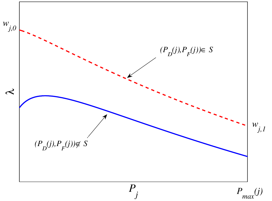
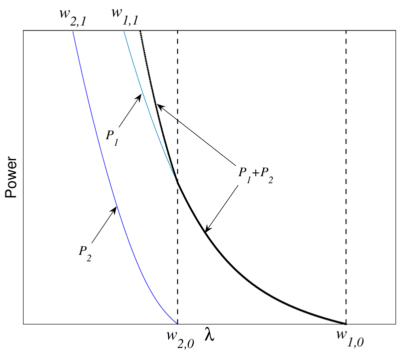
For sensor operating at , we can see that, when , we have , , and . Sensor starts to get positive power allocation when , and in this case the constraint is inactive (). is monotonically decreasing with increasing , as long as . This can be easily verified using Lemma 3 since is always non-positive for . When , is now “clamped” at , so we have and .
This case is depicted as the dashed line in Figure 6. Regardless of the value of , we can easily verify that there is always a one-to-one mapping (through (50) or (IV)) between and , and is nondecreasing with decreasing .
We have the following observations based on the above analysis. (1) If all the sensors operate at , , there is a one-to-one mapping between and , and is nondecreasing with decreasing . (2) The sensors get positive power allocation with increasing power budget (hence decreasing ) in a sequential fashion, and it is determined by .
The above observations with a two-sensor case are illustrated in Figure 6. Based on the observations, the solution can be found through a “weighted waterfilling” procedure, specified by the following algorithm. Initially the sensors send their local detection quality to the FC, and then the algorithm is executed at the FC.
Algorithm 1:
- (1)
The FC estimates the channel power gain of the sensors and the noise variance .
- (2)
- (3)
The FC finds the largest such that , and assigns and . If , the FC sets . The rest of the algorithm conducts a simple line search on between and such that .
- (4)
If , where is a small positive number, the algorithm goes to (5). Otherwise, the FC stops the algorithm and broadcasts the desired power allocations to the sensors.
- (5)
The FC sets , following bisection rule. If , the FC sets . Otherwise, the FC sets . The algorithm goes to (4).
Algorithm 1 can be easily seen to converge because of the monotonicity between total power budget and . And the simple line search of between and should converge very quickly [2].
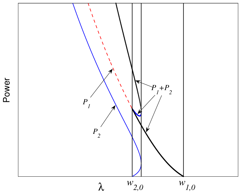
If sensor operates at , is monotonically increasing with when is small and is monotonically decreasing with when grows larger. This is because is negative and , , and are nonnegative in (IV). Thus is positive, and will eventually become negative with sufficiently large. Therefore, has a single local maximum at some , and it is possible that (IV) has two solutions for for a single . This case is also shown in Figure 6.
If one or more sensors operate at , the monotonicity and one-to-one mapping between and may be invalid, as shown in Figure 6. Therefore, the computationally efficient Algorithm 1 does not work for this case. The solution can still be obtained from general constrained optimization techniques, such as the interior point method [2][4].
V Simulations
In this section, numerical results are provided to illustrate the power allocation scheme developed in this paper. In the simulations, we consider the following settings. There are sensors scattered around an FC and the distances from the sensors to the FC are . The pathloss of signal power at the FC from sensor follows the Motley-Keenan pathloss model (expressed in dB) without the wall and floor attenuation factor [23]:
| (60) |
where is a constant set to 55 dB, and is also a constant set to 1 m in the simulations. Here, is the pathloss exponent, which is set to for free space propagation. The channel power gain for sensor is in dB. The noise variance at the FC is dBm, and we assume the noise covariance matrix is . The maximum transmitting power of each sensor is mW (3 dBm). The total power budget in the simulations will be below or equal to mW, otherwise each sensor will just use maximum transmitting power (a trivial case). All the sensors perform Neyman-Pearson detection with false alarm probabilities set to , . The detection probabilities may vary according to their local observation qualities. The FC also uses a Neyman-Pearson detector targeting the same false alarm probability as the local sensors22 2 The operation points in terms of targeted false alarm probabilities of the detectors at the sensors and the FC can be designed to be different from one another, and the analysis in this paper does not require the false alarm probabilities to be the same. The optimal design of the operating points of the detectors is beyond the scope of this paper, and we use the same false alarm probability for the sake of simplicity., i.e., .
We will investigate three scenarios: 1) two sensors with orthogonal MIMO channels. 2) two sensors with non-orthogonal MIMO channels. 3) ten sensors with orthogonal MIMO channels.
V-A Two Sensors with orthogonal channels
Two sensors are located m and m away from the FC, and communicate with the FC through orthogonal channels. Channel gains and are calculated by (60), and are -61 dB and -69 dB respectively.
We will consider four cases with various local detection quality combinations.
In Case V-A1 one sensor does not operate in region , so the interior point optimization algorithm is used in this case. In Case V-A2, Case V-A3, and Case V-A4, both sensors operate in region , thus Algorithm 1 is used. The total power budget varies from -14 dBm to 6 dBm (when each sensor transmits at full power 2 mW).
In addition to the proposed power allocation, we also include an equal power allocation and an equal received SNR power allocation for comparison. The equal power allocation simply distributes power equally among the sensors, without considering channel or local detection quality. The equal received SNR power allocation considers channel quality only and distributes power among sensors in such a way that the received signals from the sensors have the same SNR.
Figure 7 shows the proposed power allocation as well as the equal power allocation and the equal received SNR power allocation, we can see that for Case V-A1 the proposed power allocation distributes all the power to sensor 2, until the maximum output power is reached for sensor 2, and then sensor 1 starts to get positive power allocation. This is because, although sensor 1 is closer to the FC (hence it has a better channel), its detection quality is much worse than that of sensor 2. For Case V-A2, the detection quality of sensor 1 is still worse than that of sensor 2, but the gap is small enough for sensor 1’s better communication channel to show difference. The proposed allocation distributes all the power to sensor 1, until the maximum output power is reached for sensor 1, and then sensor 2 starts to get power allocation. For Case V-A3 and Case V-A4, sensor 1 has a better communication channel and equal or better local detection quality, so it is not surprising to see that the proposed allocation distributes power to sensor 1 as much as possible, and these two cases have the same power allocation as Case V-A2. The waterfilling effect of the proposed power allocation is obvious in this scenario. The equal power allocation and the equal received SNR allocation do not change between the four cases because they are not affected by the local detection quality.


Recall that the proposed power allocation scheme is based on the J-divergence instead of detection probability and false alarm probability. Furthermore, the J-divergence between two Gaussian mixture distributions, i.e., that of the received signals at the FC under the two hypotheses, is approximated in this optimization by the J-divergence between two Gaussian distributions, with the same means and covariance matrices as the Gaussian mixtures. We next show the quality of this approximation.
Figure 8 shows the optimal power allocation found by simulations. The FC uses a Neyman-Pearson detector based on the likelihood ratio of the received signal . The optimal power allocation is the one that produces the highest for a given total power budget. The optimal power allocation is found by a brute-force grid search in a two dimensional space of all possible power allocations. For each possible power allocation point, Monte Carlo runs are used to provide the corresponding .
We can see that the simulated optimal power allocations in Figure 8 perfectly match the proposed power allocations in Figure 7.
The contours of the approximated J-divergence (used as the objective function to develop the proposed power allocation) and the simulated for Case V-A3 are plotted in Figure 11 and Figure 11. The contours for the other cases are similar and are omitted due to limited space. We can see from Figure 11 and Figure 11 that the two contours match each other well at any power allocation point in this scenario, including the case in which either sensor transmits at full power (2 mW or equivalently 3 dBm). When sensor 1 transmits at full power (3 dBm), the corresponding received SNR is about 12 dB. So we can see the approximation works well in this scenario even with received SNR as high as 12 dB. This is the reason for the perfect match between the proposed allocation and the simulated optimal allocation.


In Figure 11-Figure 14, we plot the detection probability at the FC as a function of the total power budget for the four cases, and for the proposed analytical and simulated optimal allocation. The performance of the proposed power allocation matches that of the simulated optimal power allocation very well in all four cases (the two curves overlay in the four figures), and it can save almost 3 dB in compared to the equal power allocation to achieve the same . The equal received SNR power allocation considers only the channel quality, so it performs even worse than the equal power allocation in Case V-A1, where optimally sensor 1 with a better channel but much worse detection quality should use less power than sensor 2. On the other hand, in Case V-A2 through Case V-A4, the equal received SNR allocation’s performance is between the proposed allocation and equal allocation.


V-B Two sensors with non-orthogonal MIMO channels
The setting here is similar to the setting in Section V-A, but the data transmission is over non-orthogonal channels. The channel matrix is given by
| (61) |
and are the same as those in Section V-A. is the interference coefficient. We consider four cases, Case V-B1 through Case V-B4, with exactly the same local detection quality combinations as those of Case V-A1 through Case V-A4. The interior point optimization algorithm is used to solve the proposed power allocation for all four cases.
Figure 15 shows the proposed power allocation as well as the equal power allocation and the equal received SNR allocation. The major difference between Figure 15 and Figure 7 in Section V-A is that the waterfilling effect in Case V-B2 through Case V-B4 is not as obvious as that in Case V-A2 through Case V-A4. The non-orthogonal channel makes the contribution from the sensors at the FC dependent. So the power allocation is less extreme in the sense that the “better” sensors take all the power.


Figure 16 shows the optimal power allocation found by simulations for the four cases. For Case V-B1 and Case V-B4, the simulated optimal power allocations in Figure 16 match the the proposed power allocations in Figure 15. For Case V-B2 and Case V-B3, the simulated optimal power allocations are different from the proposed power allocation in higher total power budget region. For these two cases, as a function of power allocation is quite “flat” in the high total power region. This can be seen from the wider gaps between contour lines in Figure 19, and from the results in Figure 22 and Figure 22 that the performance of the proposed power allocation is still very close to that of the simulated power allocation. So the artifact of Monte Carlo trials is more pronounced, and explains the difference between the proposed power allocations and the simulated optimal power allocation in the high total power region for Case V-B2 and Case V-B3.
The contours of the approximated J-divergence and the simulated for Case V-B2 are plotted in Figure 19 and Figure 19. The two contours match each other well, but the artifact of Monte Carlo trials in Figure 19 is obvious, as discussed above.


In Figure 19-Figure 22, we plot the detection probability at the FC as a function of the total power budget , for the four cases. The performance of the proposed power allocation matches that of the simulated optimal power allocation very well in all four cases (the two curves overlay in the four figures). Compared to Figure 11-Figure 14 in Section V-A, the performance gap between the proposed power allocation and the equal power allocation (as well as the equal received SNR allocation) is slightly narrower.


V-C Ten sensors with orthogonal MIMO channels
Here we consider ten sensors scattered around an FC. We will investigate five cases, according to various sensor distance and detection probability combinations. In Case V-C1, Case V-C2, and Case V-C4, some of the sensors do not operate in region , so the interior point optimization algorithm is used in these three cases. In Case V-C3 and Case V-C5, all the sensors operate in region , thus Algorithm 1 is used. The total power budget varies from -7 dBm to 13 dBm (when each sensor transmits at full power 2 mW).
V-C1 Case V-C1
The distance between sensor and the FC is m, e.g. m and m. Sensor has detection probability of , e.g. and . In this case, sensors closer to the FC have worse detection probability.
| (dBm) | 1 | 2 | 3 | 4 | 5 | 6 | 7 | 8 | 9 | 10 |
|---|---|---|---|---|---|---|---|---|---|---|
| -7.0 | 0 | 0 | 0 | 0 | 0 | 7 | 15 | 21 | 26 | 31 |
| -2.8 | 0 | 0 | 0 | 0 | 6 | 11 | 16 | 19 | 23 | 25 |
| 3.5 | 0 | 0 | 0 | 5 | 9 | 12 | 15 | 17 | 20 | 22 |
| 8.8 | 0 | 3 | 7 | 9 | 10 | 11 | 13 | 14 | 16 | 17 |
| 13 | 10 | 10 | 10 | 10 | 10 | 10 | 10 | 10 | 10 | 10 |
| (dBm) | 1 | 2 | 3 | 4 | 5 | 6 | 7 | 8 | 9 | 10 |
|---|---|---|---|---|---|---|---|---|---|---|
| -7.0 | 100 | 0 | 0 | 0 | 0 | 0 | 0 | 0 | 0 | 0 |
| -2.8 | 74 | 26 | 0 | 0 | 0 | 0 | 0 | 0 | 0 | 0 |
| 3.5 | 36 | 23 | 15 | 10 | 7 | 5 | 3 | 1 | 0 | 0 |
| 8.8 | 18 | 14 | 12 | 10 | 9 | 8 | 8 | 7 | 7 | 7 |
| 13 | 10 | 10 | 10 | 10 | 10 | 10 | 10 | 10 | 10 | 10 |
The percentage of the total power budget allocated to each sensor is shown in Table I. When is low, more power is distributed to sensors farther away from the FC. Intuitively this is because even though sensors closer to the FC have good channel gain, their local detection qualities are much worse than those of the farther sensors. With increases, power is distributed more evenly among the sensors, because some sensors have already reached their maximum output power. Eventually, when the total power budget reaches 13 dBm, every sensor transmits at dBm.
Figure 25 shows that the approximated and actual (by Monte Carlo simulation) J-divergences are very close even when every sensor is transmitting at full power. The maximum received SNR of the closest sensor at the FC is about 12 dB. Similar to Section V-A, we can see that the approximation in J-divergence works well with SNR as high as 12 dB.
Figure 25 shows the simulated detection probability at the FC of the proposed power allocation and the equal power allocation33 3 For this scenario with 10 sensors, the complexity is too high to find the optimal power allocation by brute-force search and simulations in a ten-dimensional space of all possible power allocations. So in this scenario, we will not include the optimal power allocation found by simulation that gives the highest .. In this case, the proposed power allocation can use about 1 dB less power than equal power allocation to reach the same detection performance at the FC.
V-C2 Case V-C2
The distance between sensor and the FC is m. Sensor has detection probability of , e.g. and . In this case, sensors closer to the FC still have worse detection probability, but the gap in local detection qualities is not as large as that in case 1.
In this case, Table II shows that when is low, more power is distributed to sensors closer to the FC. The advantage in channel gain of sensors closer to the FC has offset their disadvantage in detection quality. The water filling effect is obvious here, and the sensors get positive power allocation in a sequential fashion.
V-C3 Case V-C3
m, and .
| (dBm) | 1 | 2 | 3 | 4 | 5 | 6 | 7 | 8 | 9 | 10 |
|---|---|---|---|---|---|---|---|---|---|---|
| -7.0 | 100 | 0 | 0 | 0 | 0 | 0 | 0 | 0 | 0 | 0 |
| -2.8 | 81 | 19 | 0 | 0 | 0 | 0 | 0 | 0 | 0 | 0 |
| 3.5 | 54 | 33 | 13 | 0 | 0 | 0 | 0 | 0 | 0 | 0 |
| 8.8 | 26 | 26 | 21 | 15 | 8 | 3 | 0 | 0 | 0 | 0 |
| 13 | 10 | 10 | 10 | 10 | 10 | 10 | 10 | 10 | 10 | 10 |
| (dBm) | 1 | 2 | 3 | 4 | 5 | 6 | 7 | 8 | 9 | 10 |
|---|---|---|---|---|---|---|---|---|---|---|
| -7.0 | 100 | 0 | 0 | 0 | 0 | 0 | 0 | 0 | 0 | 0 |
| -2.8 | 100 | 0 | 0 | 0 | 0 | 0 | 0 | 0 | 0 | 0 |
| 3.5 | 73 | 27 | 0 | 0 | 0 | 0 | 0 | 0 | 0 | 0 |
| 8.8 | 26 | 26 | 26 | 15 | 7 | 0 | 0 | 0 | 0 | 0 |
| 13 | 10 | 10 | 10 | 10 | 10 | 10 | 10 | 10 | 10 | 10 |
V-C4 Case V-C4
m, and . In this case, the sensors closer to the FC have advantage in both channel gain and local detection quality. So Table IV power allocation is even more biased toward sensors closer to the FC compared with Case V-C3.
In Figure 31, the approximated and actual J-divergences have more difference than the previous three cases, but their shapes are still quite similar. Figure 31 shows that the proposed power allocation consumes only less than 25% (has more than 6 dB saving) of the total power used by the equal power allocation to achieve the same detection performance at the FC.
V-C5 Case V-C5
m, and . In this case, all sensors have the same detection probability and distance from the FC. This case serves as a sanity check because intuitively the sensors should always have equal power allocation in this case. Table V and Figure 31 verify this intuition.
| (dBm) | 1 | 2 | 3 | 4 | 5 | 6 | 7 | 8 | 9 | 10 |
|---|---|---|---|---|---|---|---|---|---|---|
| -7.0 | 10 | 10 | 10 | 10 | 10 | 10 | 10 | 10 | 10 | 10 |
| -2.8 | 10 | 10 | 10 | 10 | 10 | 10 | 10 | 10 | 10 | 10 |
| 3.5 | 10 | 10 | 10 | 10 | 10 | 10 | 10 | 10 | 10 | 10 |
| 8.8 | 10 | 10 | 10 | 10 | 10 | 10 | 10 | 10 | 10 | 10 |
| 13 | 10 | 10 | 10 | 10 | 10 | 10 | 10 | 10 | 10 | 10 |


VI Conclusions
In this paper we have studied the problem of optimal power allocation for distributed detection over MIMO channels in wireless sensor networks. Our contribution is novel compared to the pervious work in the following senses: (1) We have considered a distributed detection system with a MIMO channel to account for non-ideal communications between the sensors and the FC. (2) We have assumed that there are a finite number of sensors and the sensors have independent but nonidentically distributed observations. (3) We also have assumed both individual and joint constraints on the power that the sensors can expend to transmit their local decisions to the FC. (4) We have developed a power allocation scheme to distribute the total power budget among the sensors so that the detection performance at the FC is optimized in terms of the J-divergence. (5) The proposed power allocation is a tradeoff between the quality of the local decisions of the sensors and the quality of the communication channels between the sensors and the FC. Simulations show that, to achieve the same detection performance at the FC, the proposed power allocation can use as little as 25% of the total power used by equal power allocation.
Appendix A Proof of Lemma 2
Appendix B Proof of Lemma 3
References
- [1] S. M. Ali and S. D. Silvey, “A general class of coefficients of divergence of one distribution from another,” J. Royal Stat. Soc., Series B, vol. 28, pp. 131-142, 1966.
- [2] D. P. Bertsekas, Nonlinear Programming, ed., Athena Scientific, Boston, 1999.
- [3] R. S. Blum, S. A. Kassam, and H. V. Poor, “Distributed detection with multiple sensors: Part II – Advanced topics,” Proc. IEEE, vol. 85, no. 1, pp. 64-79, Jan. 1997.
- [4] S. Boyd and L. Vandenberghe, Convex Optimization, John Wiley & Sons, Inc., New York, 1991.
- [5] B. Chen, R. Jiang, T. Kasetkasem, and P. K. Varshney, “Channel aware decision fusion in wireless sensor networks,” IEEE Trans. Signal Processing, vol. 52, no. 12, pp. 34543458, Dec. 2004.
- [6] B. Chen and P. K. Willett, “On the optimality of the likelihood-ratio test for local sensor decision rules in the presence of nonideal channels,” IEEE Trans. Inform. Theory, vol. 51, no. 2, pp. 693699, Feb. 2005.
- [7] J. F. Chamberland and V. V. Veeravalli, “Decentralized detection in sensor networks,” IEEE Trans. Signal Processing, vol. 51, no. 2, pp. 407-416, Feb. 2003.
- [8] J. F. Chamberland and V. V. Veeravalli, “Asymptotic results for decentralized detection in power constrained wireless sensor networks,” IEEE Journal on Selected Areas in Communications, vol. 22, no. 6, pp. 1007-1015, Aug. 2004.
- [9] J. F. Chamberland and V. V. Veeravalli, “How dense should a sensor network be for detection with correlated observations?” IEEE Trans. Inform. Theory, vol. 52, no. 11, pp. 50995106, Nov. 2006.
- [10] J. F. Chamberland and V. V. Veeravalli, “Wireless sensors in distributed detection applications,” IEEE Signal Processing Magazine, vol. 24, no. 3, pp. 16-25, May 2007.
- [11] T. Cover and J. Thomas, Elements of Information Theory, John Wiley & Sons, Inc., New York, 1991.
- [12] I. Csiszár and J. Körner, Information Theory: Coding Theorems for Discrete Memoryless Systems, Akadémiai Kaidó, Budapest, 1981.
- [13] T. M. Duman and M. Salehi, “Decentralized detection over multiple-access channels,” IEEE Trans. Aerosp. Electron. Syst., vol. 34, no. 2, pp. 469-476, Apr. 1998.
- [14] G. H. Golub and C. F. Van Loan, Matrix Computations, Johns Hopkins University Press, Baltimore, MD, 1996.
- [15] S. K. Jayaweera, “Bayesian fusion performance and system optimization for distributed stochastic Gaussian signal detection under communication constraints,” IEEE Trans. Signal Processing, vol. 55, no. 4, pp. 1238-1250, Apr. 2007.
- [16] H. Jeffreys, “An invariant form for the prior probability in estimation problems,” Proc. Roy. Soc. A., vol. 186, pp. 453-461, 1946.
- [17] T. Kailath, “The divergence and Bhattacharyya distance measures in signal selection,” IEEE Trans. Communication Technology, vol. 15, No. 2, pp. 52-60, Feb. 1967.
- [18] H. Kobayashi and J. B. Thomas, “Distance measures and related criteria,” Proc. Fifth Annual Allerton Conf. Circuit and System Theory, pp. 491-500, Oct. 1967.
- [19] H. Kobayashi, “Distance measures and asymptotic relative efficiency,” IEEE Trans. Inform. Theory, vol. 16, No. 3, pp. 288-291, May 1970.
- [20] K. Liu and A.M. Sayeed, “Type-based decentralized detection in wireless sensor networks,” IEEE Trans. Signal Processing, vol. 55, no. 5, pp. 1899-1910, May 2007.
- [21] G. Mergen, V. Naware, and L. Tong, “Asymptotic detection performance of type-based multiple access over multiaccess fading channels,” IEEE Trans. Signal Processing, vol. 55, no. 3, pp. 1081-1092, Mar. 2007.
- [22] P. J. Moreno, P. P. Ho, and N. Vasconcelos, “A Kullback-Leibler divergence based kernel for SVM classification in multimedia applications,” Advances in Neural Information Processing Systems, vol. 16, pp. 1385-1393, 2003.
- [23] A. J. Motley and J. P. Keenan, “Personal communication radio coverage in buildings at 900 MHz and 1700 MHz,” Electronics Letters, vol. 24, pp. 763-764, 1988.
- [24] R. Niu, B. Chen, and P. K. Varshney, “Fusion of decisions transmitted over Rayleigh fading channels in wireless sensor networks,” IEEE Trans. Signal Processing, vol. 54, no. 3, pp. 1018-1027, Mar. 2006.
- [25] H. V. Poor, An Introduction to Signal Detection and Estimation, Springer, New York, 1994.
- [26] H. V. Poor and J. B. Thomas, “Applications of Ali-Silvey distance measures in the design of generalized quantizers for binary decision systems,” IEEE Trans. Commun., vol. 25, no. 9, pp. 893-900, Sept. 1977.
- [27] J. B. Predd, S. R. Kulkarni, and H. V. Poor, “Consistency in models for distributed learning under communication constraints,” IEEE Trans. Inform. Theory, vol. 52, no. 1, pp. 52-63, Jan. 2006.
- [28] C. Rago, P. Willett, and Y. Bar-Shalom, “Censoring sensors: A low-communication-rate scheme for distributed detection,” IEEE Trans. Aerosp. Electron. Syst., vol. 32, no. 2, pp. 554-568, Apr. 1996.
- [29] Y. Singer and M. K. Warmuth, “Batch and on-line parameter estimation of Gaussian mixtures based on the joint entropy,” Advances in Neural Information Processing Systems, vol. 11, pp. 578-584, 1998.
- [30] D. Tse and P. Viswanath Fundamentals of Wireless Communication, Cambridge University Press: Cambeidge, UK, 2004.
- [31] J. N. Tsitsiklis, “Decentralized detection,” Advances in Statistical Signal Proccessing, Signal Detection, vol. 2, H. V. Poor and J. B. Thomas, Eds, pp. 297-344, JAI Press, Greenwich, CT, 1993.
- [32] P. K. Varshney, Distributed Detection and Data Fusion, Springer, New York, 1996.
- [33] R. Viswanathan and P. K. Varshney, “Distributed detection with multiple sensors: Part I – Fundamentals,” Proc. IEEE, vol. 85, no. 1, pp. 54-63, Jan. 1997.
- [34] S. Verdú, Multiuser Detection, Cambridge University Press: Cambridge, UK, 1998.
- [35] X. Wang and H. V. Poor, Wireless Communication Systems: Advanced Techniques for Signal Reception, Prentice-Hall: Upper Saddle River, NJ, 2004.