NLC-2 graph recognition and isomorphism

Vincent Limouzy Fabien de Montgolfier Michaël Rao

Abstract

NLC-width is a variant of clique-width with many application in graph algorithmic. This paper is devoted to graphs of NLC-width two. After giving new structural properties of the class, we propose a $O(n^{2}m)$ -time algorithm, improving Johansson’s algorithm [14]. Moreover, our alogrithm is simple to understand. The above properties and algorithm allow us to propose a robust $O(n^{2}m)$ -time isomorphism algorithm for NLC-2 graphs. As far as we know, it is the first polynomial-time algorithm.

¹¹footnotetext: LIAFA, Université Paris 7. {limouzy,fm,rao}@liafa.jussieu.fr. Research supported by the French ANR project “Graph Decompositions and Algorithms (GRAAL)”

1 Introduction

NLC-width is a graph parameter introduced by Wanke [16]. This notion is tightly related to clique-width introduced by Courcelle et al. [2]. Both parameters were introduced to generalise the well known tree-width. The motivation on research about such width parameter is that, when the width (NLC-, clique- or tree-width) is bounded by a constant, then many NP-complete problems can be solved in polynomial (even linear) time, if the decomposition is provided.

Such parameters give insights on graph structural properties. Unfortunately, finding the minimum NLC-width of the graph was shown to be NP-hard by Gurski et al. [12]. Some results however are known. Let NLC- $k$ be the class of graph of NLC width bounded by $k$ . NLC-1 is exactly the class of cographs. Probe-cographs, bi-cographs and weak-bisplit graphs [9] belong to NLC-2. Johansson [14] proved that recognising NLC-2 graphs is polynomial and provided an $O(n^{4}\log(n))$ recognition algorithm. Complexity for recognition of NLC- $k$ , $k\geq 3$ , is still unknown.

In this paper we improve Johansson’s result down to $O(n^{2}m)$ . Our approach relies on graph decompositions. We establish the tight links that exist between NLC-2 graphs and the so-called modular decomposition, split decomposition, and bi-join decomposition.

NLC-2 can be defined as a graph colouring problem. Unlike NLC- $k$ classes, for $k\geq 3$ , recolouring is useless for prime NLC-2 graphs. That allow us to propose a canonical decomposition of bi-coloured NLC-2 graphs, defined as certain bi-coloured split operations. This decomposition can be computed in $O(nm)$ time if the colouring is provided. If a graph is prime, there using split and bi-join decompositions, we show that there is at most $O(n)$ colourings to check. Finally, modular decomposition properties allow to reduce NLC-2 graph decomposition to prime NLC-2 graph decomposition. Section 3 explains this $O(n^{2}m)$ -time decomposition algorithm.

In Section 4 is proposed an isomorphism algorithm. Using modular, split and bi-join decompositions and the canonical NLC-2 decomposition, isomorphism between two NLC-2 graphs can be tested in $O(n^{2}m)$ time.

2 Preliminaries

A graph $G=(V,E)$ is pair of a set of vertices $V$ and a set of edges $E$ . For a graph $G$ , $V(G)$ denote its set of vertices, $E(G)$ its set of edges, $n(G)=|V(G)|$ and $m(G)=|E(G)|$ (or $V$ , $E$ , $n$ and $m$ if the graph is clear in the context). $N(x)=\{y\in V:\{x,y\}\in E\}$ denotes the neighbourhood of the vertex $x$ , and $N[x]=N(v)\cup\{v\}$ . For $W\subseteq V$ , $G[W]=(W,E\cap W^{2})$ denote the graph induced by $W$ . Let $A$ and $B$ be two disjoint subsets of $V$ . Then we note $A~\text{\textcircled{\footnotesize 1}}~B$ if for all $(a,b)\in A\times B$ , then $\{a,b\}\in E$ , and we note $A~\text{\textcircled{\footnotesize 0}}~B$ if for all $(a,b)\in A\times B$ , then $\{a,b\}\not\in E$ . Two graphs $G=(V,E)$ and $G^{\prime}=(V^{\prime},E^{\prime})$ are isomorphic (noted $G\simeq G^{\prime}$ ) if there is a bijection $\varphi:V\rightarrow V^{\prime}$ such that $\{x,y\}\in E\Leftrightarrow\{\varphi(x),\varphi(y)\}\in E^{\prime}$ , for all $u,v\in V$ .

A $k$ -labelling (or labelling) is a function $l:V\to\{1,\ldots,k\}$ . A $k$ -labelled graph is a pair of a graph $G=(V,E)$ and a $k$ -labelling $l$ on $V$ . It is denoted by $(G,l)$ or by $(V,E,l)$ . Two labelled graphs $(V,E,l)$ and $(V^{\prime},E^{\prime},l^{\prime})$ are isomorphic if there is a bijection $\varphi:V\to V^{\prime}$ such that $\{u,v\}\in E\Leftrightarrow\{\varphi(x),\varphi(y)\}\in E^{\prime}$ and $l(u)=l^{\prime}(\varphi(u))$ for all $u,v\in V$ .

NLC- $k$ classes.

Let $k$ be a positive integer. The class of NLC- $k$ graphs is defined recursively by the following operations.

•

For all $i\in\{1,\ldots,{k}\}$ , $\cdot({i})$ is in NLC- $k$ , where $\cdot({i})$ is the graph with one vertex labelled $i$ .

•

Let $G_{1}=(V_{1},E_{1},l_{1})$ and $G_{2}=(V_{2},E_{2},l_{2})$ be NLC- $k$ and let $S\subseteq{\{1,\ldots,{k}\}}^{2}$ . Then $G_{1}\times_{S}G_{2}$ is in NLC- $k$ , where

$G_{1}\times_{S}G_{2}=(V,E,l)$ with $V=V_{1}\cup V_{2}$ ,

E=E_{1}\cup E_{2}\cup\{\{u,v\}:u\in V_{1},v\in V_{2},(l_{1}(u),l_{2}(v))\in S\}

\text{and for all $u\in V$, }l(u)=\begin{cases}l_{1}(u)\text{ if $u\in V_{1}$}\\ l_{2}(u)\text{ if $u\in V_{2}$.}\end{cases}

•

Let $R:\{1,\ldots,{k}\}\rightarrow\{1,\ldots,{k}\}$ and $G=(V,E,l)$ be NLC- $k$ . Then $\rho_{R}(G)$ is in NLC- $k$ , where $\rho_{R}(G)=(V,E,l^{\prime})$ such that $l^{\prime}(u)=R(l(u))$ for all $u\in V$ .

A graph is NLC- $k$ if there is a $k$ -labelling of $G$ such that $(G,l)$ is in NLC- $k$ . A $k$ -labelled graph is NLC- $k$ $\rho$ -free if it can be constructed without the $\rho_{R}$ operation.

Modules and modular decomposition.

A module in a graph is a non-empty subset $X\subseteq V$ such that for all $u\in V\setminus X$ , then either $N(u)\cap X=\emptyset$ or $X\subseteq N(u)$ . A module is trivial if $|X|\in\{1,|V|\}$ . A graph is prime (w.r.t. modular decomposition) if all its modules are trivial. Two sets $X$ and $X^{\prime}$ overlap if $X\cap X^{\prime}$ , $X\setminus X^{\prime}$ and $X^{\prime}\setminus X$ are non-empty. A module $X$ is strong if there is no module $X^{\prime}$ such that $X$ and $X^{\prime}$ overlap. Let $\mathcal{M}^{\prime}(G)$ be the set of modules, let $\mathcal{M}(G)$ be the set of strong modules of $G$ , and let $\mathcal{P}(G)=\{M_{1},\ldots,M_{k}\}$ be the maximal (w.r.t. inclusion) members of $\mathcal{M}(G)\setminus\{V\}$ .

Theorem 1.

[11] Let $G=(V,E)$ be a graph such that $|V|\geq 2$ . Then:

•

if $G$ is not connected, then $\mathcal{P}(G)$ is the set of connected components of $G$ ,
•

if $\overline{G}$ is not connected, then $\mathcal{P}(G)$ is the set of connected components of $\overline{G}$ ,
•

if $G$ and $\overline{G}$ are connected, then $\mathcal{P}(G)$ is a partition of $V$ and is formed with the maximal members of $\mathcal{M}^{\prime}\setminus\{V\}$ .

In all cases, $\mathcal{P}(G)$ is a partition of $V$ , and $G$ can be decomposed into $G[M_{1}],\ldots,G[M_{k}]$ . The characteristic graph $G^{*}$ of a graph $G$ is the graph of vertex set $\mathcal{P}(G)$ and two $P,P^{\prime}\in\mathcal{P}(G)$ are adjacent if there is an edge between $P$ and $P^{\prime}$ in $G$ (and so there is no non-edges since $P$ and $P^{\prime}$ are two modules). The recursive decomposition of a graph by this operation gives the modular decomposition of the graph, and can be represented by a rooted tree, called the modular decomposition tree. It can be computed in linear time [15]. The nodes of the modular decomposition tree are exactly the strong modules, so in the following we make no distinction between the modular decomposition of $G$ and $\mathcal{M}(G)$ . Note that $|\mathcal{M}(G)|\leq 2\times n-1$ . For $M\in\mathcal{M}(G)$ , let $G_{M}=G[M]$ and $G^{*}_{M}$ its characteristic graph.

Lemma 2.

[14] Let $G$ be a graph. $G$ is NLC- $k$ if and only if every characteristic graph in the modular decomposition of $G$ is NLC- $k$ .

Moreover, a NLC- $k$ expression for $G$ can be easily constructed from the modular decomposition and from NLC- $k$ expressions of prime graphs. On prime graphs, NLC-2 recognition is easier:

Lemma 3.

[14] Let $G$ be a prime graph. Then $G$ is NLC-2 if and only if there is a $2$ -labelling $l$ such that $(G,l)$ is NLC-2 $\rho$ -free.

Bi-partitive family.

A bipartition of $V$ is a pair $\{X,Y\}$ such that $X\cap Y=\emptyset$ , $X\cup Y=V$ and $X$ and $Y$ are both non empty. Two bipartitions $\{X,Y\}$ and $\{X^{\prime},Y^{\prime}\}$ overlap if $X\cap Y$ , $X\cap Y^{\prime}$ , $X^{\prime}\cap Y$ and $X^{\prime}\cap Y^{\prime}$ are non empty. A family $\mathcal{F}$ of bipartitions of $V$ is bipartitive if (1) for all $v\in V$ , $\{\{v\},V\setminus\{v\}\}\in\mathcal{F}$ and (2) for all $\{X,Y\}$ and $\{X^{\prime},Y^{\prime}\}$ in $\mathcal{F}$ such that $\{X,Y\}$ and $\{X^{\prime},Y^{\prime}\}$ overlap, then $\{X\cap X^{\prime},Y\cup Y^{\prime}\}$ , $\{X\cap Y^{\prime},Y\cup X^{\prime}\}$ , $\{Y\cap X^{\prime},X\cup Y^{\prime}\}$ , $\{Y\cap Y^{\prime},X\cup X^{\prime}\}$ and $\{X\Delta X^{\prime},X\Delta Y^{\prime}\}$ are in $\mathcal{F}$ (where $X\Delta Y=(X\setminus Y)\cup(Y\setminus X)$ ). Bipartitive families are very close to partitive families [1], which generalise properties of modules in a graph.

A member $\{X,Y\}$ of a bipartitive family $\mathcal{F}$ is strong if there is no $\{X^{\prime},Y^{\prime}\}$ such that $\{X,Y\}$ and $\{X^{\prime},Y^{\prime}\}$ overlap. Let $T$ be a tree. For an edge $e$ in the tree, $\{C_{e}^{1},C_{e}^{2}\}$ denote the bipartition of leaves of $T$ such that two leaves are in the same set if and only if the path between them avoids $e$ . Similarly, for an internal node $\alpha$ , $\{C_{\alpha}^{1},\ldots,C_{\alpha}^{d(\alpha)}\}$ denote the partition of leaves of $T$ such that two leaves are in the same set if and only if the path between them avoid $\alpha$ .

Theorem 4.

[3] Let $\mathcal{F}$ be a bipartitive family on $V$ . Then there is an unique unrooted tree $T$ , called the representative tree of $\mathcal{F}$ , such that the set of leaves of $T$ is $V$ , the internal nodes of $T$ are labelled degenerate or prime, and
- for every edge $e$ of $T$ , $\{C_{e}^{1},C_{e}^{2}\}$ is a strong member of $\mathcal{F}$ , and there is no other strong member in $\mathcal{F}$ ,
- for every node $\alpha$ labelled degenerate, and for every $\emptyset\subsetneq I\subsetneq\{1,\ldots,d(\alpha)\}$ ,
$\{\cup_{i\in I}C_{\alpha}^{i},V\setminus\cup_{i\in I}C_{\alpha}^{i}\}$ is in $\mathcal{F}$ , and there is no other member in $\mathcal{F}$ .

Split decomposition.

A split in a graph $G=(V,E)$ is a bipartition $\{X,Y\}$ of $V$ such that the set of vertices in $X$ having a neighbour in $Y$ have the same neighbourhood in $Y$ (i.e., for all $u,v\in X$ such that $N(u)\cap Y\neq\emptyset$ and $N(v)\cap Y\neq\emptyset$ , then $N(u)\cap Y=N(v)\cap Y$ ). A co-split in a graph $G$ is a split in $\overline{G}$ . The family of split in a connected graph is a bipartitive family [4]. The split decomposition tree is the representative tree of the family of splits, and can be computed in linear time [5]. Let $\alpha$ be an internal node of the split decomposition tree of a connected graph $G$ . For all $i\in\{1,\ldots,d(\alpha)\}$ let $v_{i}\in C_{\alpha}^{i}$ such that $N(v_{i})\setminus C_{\alpha}^{i}\neq\emptyset$ . Since $G$ is connected, such a $v_{i}$ always exists. $G[\{v_{1},\ldots,v_{d(\alpha)}\}]$ denote the characteristic graph of $\alpha$ . The characteristic graph of a degenerate node is a complete graph or a star [4].

Bi-join decomposition.

A bi-join in a graph is a bipartition $\{X,Y\}$ such that for all $u,v\in X$ , $\{N(u)\cap Y,Y\setminus N(u)\}=\{N(v)\cap Y,Y\setminus N(v)\}$ . The family of bi-joins in a graph is bipartitive. The bi-join decomposition tree is the representative tree of the family of bi-joins, and can be computed in linear time [7, 8]. Let $\alpha$ be an internal node of the bi-join decomposition tree of a graph $G$ . For all $i\in\{1,\ldots,d(\alpha)\}$ let $v_{i}\in C_{\alpha}^{i}$ . $G[\{v_{1},\ldots,v_{d(\alpha)}\}]$ denote the characteristic graph of $\alpha$ . The characteristic graph of a degenerate node is a complete bipartite graph or a disjoint union of two complete graphs [7, 8].

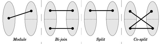
Refer to caption — Figure 1: A module, a bi-join, a split and a co-split

3 Recognition of NLC-2 graphs

3.1 NLC-2 $\rho$ -free canonical decomposition

In this section, $G=(V,E,l)$ is a 2-labelled graph such that every mono-coloured module (i.e. a module $M$ such that $\forall v,v^{\prime}\in M$ , $l(v)=l(v^{\prime})$ ) has size $1$ . A couple $(X,Y)$ is a cut if $X\cup Y=V$ , $X\cap Y=\emptyset$ , $X\neq\emptyset$ and $Y\neq\emptyset$ . Let $S\subseteq\{1,2\}\times\{1,2\}$ . A cut $(X,Y)$ is a $S$ -cut of $G$ if for all $u\in X$ and $v\in Y$ , then $\{u,v\}\in E$ if and only if $(l(u),l(v))\in S$ . For $S\subseteq\{1,2\}\times\{1,2\}$ let $\mathcal{F}_{S}(G)$ be the set of $S$ -cut of $G$ .

Definition 5 (Symmetry).

We say that $S\in\{1,2\}\times\{1,2\}$ is symmetric if $(1,2)\in S\iff(2,1)\in S$ , otherwise we say that $S$ is non-symmetric.

Definition 6 (Degenerate property).

A family $\mathcal{F}$ of cuts has the degenerate property if there is a partition $\mathcal{P}$ of $V$ such that for all $\emptyset\subsetneq\mathcal{X}\subsetneq\mathcal{P}$ , $(\bigcup_{X\in\mathcal{X}}X,\bigcup_{Y\in\mathcal{P}\setminus\mathcal{X}}Y)$ is in $\mathcal{F}$ , and there is no others cut in $\mathcal{F}$ .

Lemma 7.

For every symmetric $S\subseteq\{1,2\}\times\{1,2\}$ , $\mathcal{F}_{S}(G)$ has the degenerate property.

Proof.

The family $\mathcal{F}_{\{\}}(G)$ has the degenerate property since $(X,Y)$ is a $\{\}$ -cut if and only if there is no edges between $X$ and $Y$ ( $\mathcal{P}$ is exactly the connected components). For $W\subseteq V$ , let $G|W=(V,E\Delta W^{2},l)$ . For $i\in\{1,2\}$ let $V_{i}=\{v\in V:l(v)=i\}$ . Let $G_{1}=G|V_{1}$ , $G_{2}=G|V_{2}$ and $G_{12}=(G|V_{1})|V_{2}$ .

•

$\mathcal{F}_{\{(1,1)\}}(G)=\mathcal{F}_{\{\}}(G_{1})$ , $\mathcal{F}_{\{(2,2)\}}(G)=\mathcal{F}_{\{\}}(G_{2})$ , $\mathcal{F}_{\{(1,1),(2,2)\}}(G)=\mathcal{F}_{\{\}}(G_{12})$ ,
•

$\mathcal{F}_{\{(1,1),(1,2),(2,1),(2,2)\}}(G)=\mathcal{F}_{\{\}}(\overline{G})$ , $\mathcal{F}_{\{(1,2),(2,1),(2,2)\}}(G)=\mathcal{F}_{\{\}}(\overline{G_{1}})$ ,
$\mathcal{F}_{\{(1,1),(1,2),(2,1)\}}(G)=\mathcal{F}_{\{\}}(\overline{G_{2}})$ , $\mathcal{F}_{\{(1,2),(2,1)\}}(G)=\mathcal{F}_{\{\}}(\overline{G_{12}})$ .

Thus for every symmetric $S\subseteq\{1,2\}\times\{1,2\}$ , $\mathcal{F}_{S}(G)$ has the degenerate property.∎

Definition 8 (Linear property).

A family $\mathcal{F}$ of cuts has the linear property if for all $(X,Y)$ and $(X^{\prime},Y^{\prime})$ in $\mathcal{F}$ , either $X\subseteq X^{\prime}$ or $X^{\prime}\subseteq X$ .

Lemma 9.

For every non-symmetric $S\subseteq\{1,2\}\times\{1,2\}$ , $\mathcal{F}_{S}(G)$ has the linear property.

Proof.

Case $S=\{(1,2)\}$ : suppose that $X\setminus X^{\prime}$ and $X^{\prime}\setminus X$ are both non-empty. Then if $u\in X\setminus X^{\prime}$ is labelled $1$ and $v\in X^{\prime}\setminus X$ is labelled $2$ , $u$ and $v$ has to be adjacent and non-adjacent, contradiction. Thus $X\setminus X^{\prime}$ and $X^{\prime}\setminus X$ are mono-coloured. Now suppose w.l.o.g. that all vertices in $X\Delta X^{\prime}$ are labelled $1$ . Then $X\Delta X^{\prime}$ is adjacent to all vertices labelled $2$ in $Y\cap Y^{\prime}$ and non adjacent to all vertices labelled $1$ in $Y\cap Y^{\prime}$ . Moreover $X\Delta X^{\prime}$ is non adjacent to all vertices in $X\cap X^{\prime}$ . Thus $X\Delta X^{\prime}$ is a mono-coloured module, and $|X\Delta X^{\prime}|\geq 2$ . Contradiction. For others non-symmetric $S$ , we bring back to case $\{(1,2)\}$ like in the proof of lemma 7. ∎

For $S\subseteq\{1,2\}\times\{1,2\}$ , let $\mathcal{P}_{S}(G)$ denote the unique partition of $V$ such that (1) for all $(X,Y)\in\mathcal{F}_{S}(G)$ and $P\in\mathcal{P}_{S}(G)$ , $P\subseteq X$ or $P\subseteq Y$ , and (2) for all $P,P^{\prime}\in\mathcal{P}$ , $P\neq P^{\prime}$ , there is a $(X,Y)\in\mathcal{F}_{S}(G)$ such that $P\subseteq X$ and $P^{\prime}\subseteq Y$ , or $P\subseteq Y$ and $P^{\prime}\subseteq X$ . For a non-symmetric $S\in\{1,2\}\times\{1,2\}$ , let $\mathcal{P}^{\prime}_{S}(G)=(P_{1},\ldots,P_{k})$ denote the unique ordering of elements in $\mathcal{P}_{S}(G)$ such that for all $(X,Y)\in\mathcal{F}_{S}(G)$ , there is a $l$ such that $X=\cup_{i\in\{1,\ldots,l\}}P_{i}$ .

Lemma 10.

If $G$ is in NLC-2 $\rho$ -free, then there is a $S\subseteq\{1,2\}\times\{1,2\}$ such that $\mathcal{F}_{S}(G)$ is non-empty.

Proof.

If $G$ is NLC-2 $\rho$ -free, then there is a $S\subseteq\{1,2\}\times\{1,2\}$ , and two graphs $G_{1}$ and $G_{2}$ such that $G=G_{1}\times_{S}G_{2}$ . Thus $(V(G_{1}),V(G_{2}))\in\mathcal{F}_{S}(G)$ and $\mathcal{F}_{S}(G)$ is non empty. ∎

Lemma 11.

Let $G=(V,E,l)$ 2-labelled graph and let $S\subseteq\{1,2\}\times\{1,2\}$ . If $G$ is NLC-2 $\rho$ -free and has no mono-coloured non-trivial module, then for all $P\in\mathcal{P}_{S}(G)$ , $G[P]$ has no mono-coloured non-trivial module.

Proof.

If $M$ is a mono-coloured module of $G[P]$ , then $M$ is a mono-coloured module of $G$ . Contradiction. ∎

Lemma 12.

Let $G=(V,E,l)$ 2-labelled graph and let $S\subseteq\{1,2\}\times\{1,2\}$ . Then $G$ is NLC-2 $\rho$ -free if and only if for all $P\in\mathcal{P}_{S}(G)$ , $G[P]$ is NLC-2 $\rho$ -free.

Proof.

The “only if” is immediate. Now suppose that for all $P\in\mathcal{P}_{S}(G)$ , $G[P]$ is NLC-2 $\rho$ -free. If $S$ is symmetric, let $\mathcal{P}_{S}(G)=\{P_{1},\ldots,P_{|\mathcal{P}_{S}(G)|}\}$ . Then $G=((G[P_{1}]\times_{S}G[P_{2}])\times_{S}\ldots\times_{S}G[P_{|\mathcal{P}_{S}(G)|}]$ , and $G$ is NLC-2 $\rho$ -free. Otherwise, if $S$ is non-symmetric, let $\mathcal{P}^{\prime}_{S}(G)=(P_{1},\ldots,P_{|\mathcal{P}_{S}(G)|})$ . Then $G=((G[P_{1}]\times_{S}G[P_{2}])\times_{S}\ldots\times_{S}G[P_{|\mathcal{P}_{S}(G)|}]$ , and $G$ is NLC-2 $\rho$ -free. ∎

The NLC-2 $\rho$ -free decomposition tree of a $2$ -labelled graph $G$ is a rooted tree such that the leaves are the vertices of $G$ , and the internal nodes are labelled by $\times_{S}$ , with $S\subseteq\{1,2\}\times\{1,2\}$ . An internal node is degenerated if $S$ is symmetric, and linear if $S$ is non-symmetric. By lemmas 10, 11 and 12, $G$ is NLC-2 $\rho$ -free if and only if it has a NLC-2 $\rho$ -free decomposition tree. This decomposition tree is not unique. But we can define a canonical decomposition tree if we fix a total order on the subsets of $\{1,2\}\times\{1,2\}$ (for example, the lexicographic order). If two graphs are isomorphic, then they have the same canonical decomposition tree. Algorithm 1 computes the canonical decomposition tree of a $2$ -labelled prime graph, or fails if $G$ is not NLC-2 $\rho$ -free.

Input: A

2

-labelled graph

G=(V,E,l)

Output: A NLC-2

\rho

-free decomposition tree, or fail if

G

is not NLC-2

\rho

-free

if $|V|=1$ then return the leaf $\cdot({l(v)})$ (where

V=\{v\}

)

Let

\mathcal{S}

be the set of subsets of

\{1,2\}\times\{1,2\}

and

\sigma

be the lexicographic order of

\mathcal{S}

foreach $S\in\mathcal{S}$ w.r.t. $\sigma$ do Compute

\mathcal{P}_{S}(G)

, and

\mathcal{P}^{\prime}_{S}(G)

S

is non-symmetric (see algorithm 2)

if $|\mathcal{P}_{S}(G)|>1$ then Create a new

\times_{S}

node

\beta

foreach $P\in\mathcal{P}_{S}(G)$ (w.r.t. $\mathcal{P}^{\prime}_{S}(G)$ if $S$ is non-symmetric) do make NLC-2

\rho

-free decomposition tree of

G[P]

be a child of

\beta

. 4 4 4 4 return the tree rooted at $\beta$ fail with Not NLC-2 $\rho$ -free

Algorithm 1 Computation of the NLC-2

\rho

-free canonical decomposition tree

Algorithm 2 computes $\mathcal{P}_{S}$ and $\mathcal{P}^{\prime}_{S}$ for a $2$ -labelled prime graph $G$ and $S\subseteq\{1,2\}\times\{1,2\}$ in linear time. We need some additional definitions for this algorithm and its proof of correctness. A bipartite graph is a triplet $(X,Y,E)$ such that $E\subseteq X\times Y$ . The bi-complement of a bipartite graph $(X,Y,E)$ is the bipartite graph $(X,Y,(X\times Y)\setminus E)$ . A bipartite trigraph (BT) is a bipartite graph with two types of edges: the join edges and the mixed edges. It is denoted by $\mathcal{B}=(X,Y,E_{j},E_{m})$ where $E_{j}$ are the set of join edges, and $E_{m}$ the set of mixed edges. A BT-module in a BT is a $M\subseteq X$ or $M\subseteq Y$ such that $M$ is a module in $(X,Y,E_{j})$ and there is no mixed edges between $M$ and $(X\cup Y)\setminus M$ . For $v\in X\cup Y$ , let $N_{j}(v)=\{u\in X\cup Y:\{u,v\}\in E_{j}\}$ and $N_{m}(v)=\{u\in X\cup Y:\{u,v\}\in E_{m}\}$ . Let $d_{j}(v)=|N_{j}(v)|$ and $d_{m}(v)=|N_{m}(v)|$ . A semi-join in a BT $(X,Y,E_{j},E_{m})$ is a cut $(A,B)$ of $X\cup Y$ , such that there is no edges between $A\cap Y$ and $B\cap X$ , and there is only join edges between $A\cap X$ and $B\cap Y$ .

In algorithm 2, $\mathcal{B}$ is obtained from the graph $G$ . Vertices of $X$ correspond to subsets of vertices labelled $1$ in $G$ , and vertices of $Y$ correspond to subsets of vertices labelled $2$ . There is a join edge between $M$ and $M^{\prime}$ in $\mathcal{B}$ if $M~\text{\textcircled{\footnotesize 1}}~M^{\prime}$ in $G$ , and there is a mixed edge between $M\in X$ and $M^{\prime}\in Y$ in $\mathcal{B}$ if there is at least an edge and a non-edge between $M$ and $M^{\prime}$ in $G$ . Such a graph $\mathcal{B}$ can easily be built in linear time from a given graph $G$ . It suffices to consider a list and an array bounded by the number of component in $G$ with the same colour. The following lemmas are close to observations in [9], but deal with BT instead of bipartite graphs (proofs are given in appendix).

Lemma 13.

Let $G=(X,Y,E_{j},E_{m})$ be a BT such that every BT-module has size $1$ . Let $(x_{1},\ldots,x_{|X|})$ be $X$ sorted by $(d_{j}(x),d_{m}(x))$ in lexicographic decreasing order. If $(A,B)$ is a semi-join of $G$ , then there is a $k\in\{0,\ldots,|X|\}$ such that $A\cap X=\{x_{1},\ldots,x_{k}\}$ .

Lemma 14.

Let $k\in\{0,\ldots,|X|\}$ and $k^{\prime}\in\{0,\ldots,|Y|\}$ . Then $(A,(X\cup Y)\setminus A)$ , where $A=\{x_{1},\ldots,x_{k},y_{1},\ldots,y_{k^{\prime}}\}$ , is a semi-join of $G$ if and only if $\sum_{i=1}^{k}d_{j}(x_{i})-\sum_{i=1}^{k^{\prime}}d_{j}(y_{i})=k\times(|Y|-k^{\prime})$ and $\sum_{i=1}^{k}d_{m}(x_{i})-\sum_{i=1}^{k^{\prime}}d_{m}(y_{i})=0$ .

Input: A

2

-labelled graph

G

, and

S\subseteq\{1,2\}\times\{1,2\}

Output:

\mathcal{P}_{S}

S

is symmetric,

\mathcal{P}^{\prime}_{S}

S

is non-symmetric

V_{i}

\leftarrow\{v:v\in V

and

l(v)=i\}

;

if $(1,1)\in S$ then

\mathcal{C}_{1}\leftarrow

co-connected components of

G[V_{1}]

;

else

\mathcal{C}_{1}\leftarrow

connected components of

G[V_{1}]

;

if $(2,2)\in S$ then

\mathcal{C}_{2}\leftarrow

co-connected components of

G[V_{2}]

;

else

\mathcal{C}_{2}\leftarrow

connected components of

G[V_{2}]

;

\mathcal{B}=(\mathcal{C}_{1},\mathcal{C}_{2},E_{j},E_{m})

\leftarrow

the bipartite trigraph between the elements of

\mathcal{C}_{1}

and

\mathcal{C}_{2}

;

if $S\cap\{(1,2),(2,1)\}=\emptyset$ then

return connected components of $(\mathcal{C}_{1},\mathcal{C}_{2},E_{j}\cup E_{m})$ 8 8 8 8 8 8 8 8 else if $S\cap\{(1,2),(2,1)\}=\{(1,2),(2,1)\}$ then

return connected components of the bi-complement of $(\mathcal{C}_{1},\mathcal{C}_{2},E_{j})$ 9 else Search all semi-joins of

\mathcal{B}

(see appendix) ;

Algorithm 2 Computation of

\mathcal{P}_{S}

and

\mathcal{P}^{\prime}_{S}

Theorem 15.

Algorithm 2 is correct and runs in linear time.

Proof.

Correctness: Suppose that $(A,B)$ is a $S$ -cut. If $(1,1)\not\in S$ , then there is no edge between $A\cap V_{1}$ and $B\cap V_{1}$ , thus $(A,B)$ cannot cut a component $\mathcal{C}_{1}$ (and similarly for $(1,1)\in S$ , and for $\mathcal{C}_{2}$ ). Now we work on the BT $\mathcal{B}=(\mathcal{C}_{1},\mathcal{C}_{2},E_{j},E_{m})$ . If $S\cap\{(1,2),(2,1)\}=\emptyset$ , then $S$ -cuts correspond exactly to connected components of $\mathcal{B}$ , and if $S\cap\{(1,2),(2,1)\}=\{(1,2),(2,1)\}$ then $S$ -cuts correspond exactly to connected components of the BT of $\overline{G}$ , which is $(\mathcal{C}_{1},\mathcal{C}_{2},(\mathcal{C}_{1}\times\mathcal{C}_{2})\setminus(E_{j}\cup E_{m}),E_{m})$ . Finally, if $S$ is non-symmetric, $S$ -cuts correspond to semi-joins of $\mathcal{B}$ (see appendix).

Complexity: It is well admitted that we can perform a BFS on a graph or its complement in linear time [13, 6]. The instructions on lines [2-2,2] can be done with a BFS on a graph or its complement. It is easy to see that we can do a BFS on the bi-complement in linear time (like a BFS on a complement graph, with two vertex lists for $X$ and $Y$ ), so instruction line 2 can be done in linear time. Finally, the operations at line 2 are done in linear time (see appendix). ∎

These results can be summarized as:

Theorem 16.

Algorithm 1 computes the canonical NLC-2 $\rho$ -free decomposition tree of a 2-labelled graph in $O(nm)$ time.

3.2 NLC-2 decomposition of a prime graph

In this section, $G$ is an unlabelled prime (w.r.t. modular decomposition) graph, with $|V|\geq 3$ .

Definition 17 ( $2$ -bimodule).

A bipartition $\{X,Y\}$ of $V$ is a $2$ -bimodule if $X$ can be partitioned into $X_{1}$ and $X_{2}$ , and $Y$ into $Y_{1}$ and $Y_{2}$ such that for all $(i,j)\in\{1,2\}\times\{1,2\}$ , then either $X_{i}~\text{\textcircled{\footnotesize 0}}~Y_{j}$ or $X_{i}~\text{\textcircled{\footnotesize 1}}~Y_{j}$ . It is easy to see that if $\{X,Y\}$ is a $2$ -bimodule if and only if $\{X,Y\}$ is a split, a co-split or a bi-join. Moreover, if $\min(|X|,|Y|)>1$ then $\{X,Y\}$ cannot be both of them in the same time (since $G$ is prime).

Let $l:V\to\{1,2\}$ be a 2-labelling. Then $s(l)$ denote the 2-labelling on $V$ such that for all $v\in V$ , $s(l)(v)=1$ if and only if $l(v)=2$ .

Definition 18 (Labelling induced by a $2$ -bimodule).

Let $\{X,Y\}$ be a $2$ -bimodule. We define the labelling $l:V\to\{1,2\}$ of $G$ induced by $\{X,Y\}$ . If $|X|=|Y|=1$ , then $l(x)=1$ and $l(y)=2$ , where $X=\{x\}$ and $Y=\{y\}$ . If $|X|=1$ , then $l(v)=1$ iff $v\in N[x]$ . Similarly if $|Y|=1$ , then $l(v)=1$ iff $v\in N[y]$ . Now we suppose $\min(|X|,|Y|)>1$ . If $\{X,Y\}$ is a split, then the set of vertices in $X$ with a neighbour $Y$ and the set of vertices in $Y$ with a neighbour in $X$ is labelled $1$ , others vertices are labelled $2$ . If $\{X,Y\}$ is a co-split, then a labelling of $G$ induced by $\{X,Y\}$ is a labelling of $\overline{G}$ induced by the split $\{X,Y\}$ . Finally if $\{X,Y\}$ is a bi-join, $l$ is such that $\{v\in X:l(v)=1\}$ is a join with $\{v\in Y:l(v)=1\}$ and $\{v\in X:l(v)=2\}$ is a join with $\{v\in Y:l(v)=2\}$ . Note that if $\{X,Y\}$ is a bi-join, then there is two possibles labelling $l_{1}$ and $l_{2}$ , with $l_{1}=s(l_{2})$ . If $\{X,Y\}$ is a $2$ -bimodule of $G$ and $l$ a labelling induced by $\{X,Y\}$ , then every mono-coloured module has size $1$ (since $G$ is prime and $|V|\geq 3$ ).

Definition 19 (Good $2$ -bimodule).

A $2$ -bimodule $\{X,Y\}$ is good if the graph $G$ with the labelling induced by $\{X,Y\}$ is NLC-2 $\rho$ -free. The following proposition comes immediately from lemma 3.

Proposition 20.

$G$ is NLC-2 if and only if $G$ has a good $2$ -bimodule.

Lemma 21.

If $G$ has a good $2$ -bimodule $\{X,Y\}$ which is a split, then $G$ has a good $2$ -bimodule which is a strong split.

Proof.

There is a node $\alpha$ in the split decomposition tree and $\emptyset\subsetneq I\subsetneq\{1,\ldots,d(\alpha)\}$ such that $\{X,Y\}=\{\cup_{i\in I}C_{\alpha}^{i},\cup_{i\not\in I}C_{\alpha}^{i}\}$ . Let $l:V\to\{1,2\}$ be the labelling of $G$ induced by $\{X,Y\}$ . For all $i\in\{1,\ldots,d(\alpha)\}$ , $(G[C_{\alpha}^{i}],{l}|_{C_{\alpha}^{i}})$ is NLC-2 $\rho$ -free (where $l|_{W}$ is the function $l$ restricted at $W$ ).

Let $l^{\prime}$ be the $2$ -labelling of $V$ such that for all $i$ , and $v\in C_{\alpha}^{i}$ , $l(v)=1$ if and only if $v$ has a neighbour outside of $C_{\alpha}^{i}$ . For all $i$ , either ${l}|_{C_{\alpha}^{i}}={l^{\prime}}|_{C_{\alpha}^{i}}$ , or $\forall v\in C_{\alpha}^{i}$ , $l(v)=2$ . Then for all $i$ , $(G[C_{\alpha}^{i}],{l^{\prime}}|_{C_{\alpha}^{i}})$ is NLC-2 $\rho$ -free, and thus $(G,l^{\prime})$ is NLC-2 $\rho$ -free. Since there is a dominating vertex in the characteristic graph of $\alpha$ , there is a $j$ such that the labelling induced by the strong split $\{C_{\alpha}^{j},V\setminus C_{\alpha}^{j}\}$ is $l^{\prime}$ . Thus the strong split $\{C_{\alpha}^{j},V\setminus C_{\alpha}^{j}\}$ is good. ∎

Previous lemma on $\overline{G}$ say that if $G$ has a good $2$ -bimodule $\{X,Y\}$ which is a co-split, then $G$ has a good $2$ -bimodule which is a strong co-split. The following lemma is similar to Lemma 21.

Lemma 22.

If $G$ has a good $2$ -bimodule $\{X,Y\}$ which is a bi-join, then $G$ has a good $2$ -bimodule which is a strong bi-join.

Input: A graph

G

Result: Yes iff

G

is NLC-2

\mathcal{S}\leftarrow

the set of strong splits, co-splits and bi-joins of

G

;

foreach $\{X,Y\}\in\mathcal{S}$ do

l

\leftarrow

the labelling of

G

induced by

\{X,Y\}

;

if $(G[X],G[Y],l)$ is NLC-2 $\rho$ -free then return Yes ;

return No ;

Algorithm 3 Recognition of prime NLC-2 graphs

Theorem 23.

Algorithm 3 recognises prime NLC-2 graphs, and its time complexity is $O(n^{2}m)$ .

Proof.

Trivially if the algorithm return Yes, then $G$ is NLC-2. On the other hand, by proposition 20, and lemmas 21 and 22, if $G$ is NLC-2, then it has a good strong $2$ -bimodule and the algorithm returns Yes.

The set $\mathcal{S}$ can be computed using algorithms for computing split decomposition on $G$ and $\overline{G}$ , and bi-join decomposition on $G$ . Note that it is not required to use a linear time algorithm for split decomposition [5]: some simpler algorithms run in $O(n^{2}m)$ [4, 10]. [7, 8] show that bi-join decomposition can be computed in linear time, using a reduction to modular decomposition. But there also, modular decomposition algorithms simpler than [15] may be used. The set $\mathcal{S}$ has $O(n)$ elements. Testing if a $2$ -bimodule is good takes $O(nm)$ using algorithm 1. So total running time is $O(n^{2}m)$ . ∎

3.3 NLC-2 decomposition

Using lemma 2, modular decomposition and algorithm 3, we get:

Theorem 24.

NLC-2 graphs can be recognised in $O(n^{2}m)$ , and a NLC-2 expression can be generated in the same time.

4 Graph isomorphism on NLC-2 graphs

4.1 Graph Isomorphism on NLC-2 $\rho$ -free prime graphs

The following propositions are direct consequences of properties (linear and degenerate) of $S$ -cuts.

Proposition 25.

Consider a symmetric $S\in\{1,2\}\times\{1,2\}$ . Two graphs $G$ and $H$ are isomorphic if and only if there is a bijection $\pi$ between $\mathcal{P}_{S}(G)$ and $\mathcal{P}_{S}(H)$ such that for all $P\in\mathcal{P}_{S}(G)$ , $G[P]$ is isomorphic to $H[\pi(P)]$ .

Proposition 26.

Let a non-symmetric $S\in\{1,2\}\times\{1,2\}$ and let $G$ and $H$ be two graphs. Let $\mathcal{P}^{\prime}_{S}(G)=(P_{1},\ldots,P_{k})$ and $\mathcal{P}^{\prime}_{S}(H)=(P^{\prime}_{1},\ldots,P^{\prime}_{k^{\prime}})$ then $G$ and $H$ are isomorphic if and only if $k=k^{\prime}$ and for all $i\in\{1,\ldots,k\}$ , $G[P_{i}]$ is isomorphic to $H[P^{\prime}_{i}]$ .

By the previous 2 propositions, two NLC-2 $\rho$ -free 2-labelled graphs $G$ and $H$ are isomorphic if and only if there is an isomorphism between their canonical NLC-2 $\rho$ -free decomposition tree which respects the order of children of linear nodes. This isomorphism can be tested in linear time, thus isomorphism of NLC-2 $\rho$ -free graphs can be done in $O(nm)$ time.

4.2 Graph isomorphism on prime NLC-2 graphs

Input: Two prime NLC-2 graphs

G

and

H

Result: Yes if

G\simeq H

, No otherwise

\mathcal{S}\leftarrow

the set of strong splits, co-splits and bi-joins of

G

;

\mathcal{S}^{\prime}\leftarrow

the set of strong splits, co-splits and bi-joins of

H

;

if there is no good $2$ -bimodule in $\mathcal{S}$ then fail with “

G

is not NLC-2’’;

\{X,Y\}\leftarrow

a good

2

-bimodule in

\mathcal{S}

;

l

\leftarrow

the labelling of

G

induced by

\{X,Y\}

;

foreach $\{X^{\prime},Y^{\prime}\}\in\mathcal{S}^{\prime}$ such that $\{X^{\prime},Y^{\prime}\}$ is good do

l^{\prime}

\leftarrow

the labelling of

H

induced by

\{X^{\prime},Y^{\prime}\}

;

if $|X|>1$ and $|Y|>1$ and $\{X,Y\}$ is a bi-join then if $(G,l)\simeq(H,l^{\prime})$ or $(G,l)\simeq(H,s(l^{\prime}))$ then return Yes ;

else if $(G,l)\simeq(H,l^{\prime})$ then return Yes ;

return No ;

Algorithm 4 Isomorphism for prime NLC-2 graphs

Theorem 27.

Algorithm 4 test isomorphism between two prime NLC-2 graphs in time $O(n^{2}m)$ .

Proof.

If the algorithm returns “yes”, then trivially $G\simeq H$ . On the other hand suppose that $G\simeq H$ and let $\pi:V(G)\to V(H)$ be a bijection such that $\{u,v\}\in E(G)$ iff $(\pi(u),\pi(v))\in E(H)$ . Then $\{X^{\prime},Y^{\prime}\}$ with $X^{\prime}=\pi(X)$ and $Y^{\prime}=\pi(Y)$ is a good $2$ -bimodule if $H$ . If $\min(|X|,|Y|)>1$ and $\{X^{\prime},Y^{\prime}\}$ is a bi-join, then by definition there is two labelling induced by $\{X,Y\}$ , and $(G,l)\simeq(H,l^{\prime})$ or $(G,l)\simeq(H,s(l^{\prime}))$ . Otherwise the labelling is unique and $(G,l)\simeq(H,l^{\prime})$ .

The sets $\mathcal{S}$ and $\mathcal{S}^{\prime}$ can be computed in $O(n^{2})$ time using linear time algorithms for computing split decomposition on $G$ and $\overline{G}$ , and bi-join decomposition on $G$ . The sets $\mathcal{S}$ and $\mathcal{S}^{\prime}$ have $O(n)$ elements. Test if a $2$ -bimodule is good take $O(nm)$ using algorithm 1, and test if two $2$ -labelled prime graphs are isomorphic take also $O(nm)$ . Thus the total running time is $O(n^{2}m)$ . ∎

4.3 Graph isomorphism on NLC-2 graphs

It is easy to show that graph isomorphism on prime NLC-2 graphs with an additional labels into $\{1,\ldots,q\}$ can be done in $O(n^{2}m)$ time. For that, we add the additional label of $v$ at the leaf corresponding to $v$ in the NLC-2 $\rho$ -free decomposition tree.

We show that we can do graph isomorphism on NLC-2 graphs in time $O(n^{2}m)$ , using the modular decomposition and algorithm 4. Let $\mathcal{M}(G)$ and $\mathcal{M}(H)$ be the modular decomposition of $G$ and $H$ . For $M\in\mathcal{M}(G)$ , let $G_{M}$ be $G[M]$ , and for $M\in\mathcal{M}(H)$ , let $H_{M}$ be $H[M]$ . Let $G^{*}_{M}$ be the characteristic graph of $G_{M}$ (note that $|V(G^{*}_{M})|$ is the number of children of $M$ in the modular decomposition tree). Let $\mathcal{M}_{(i,*)}=\{M\in\mathcal{M}(G)\cup\mathcal{M}(H):|M|=i\}$ , let $\mathcal{M}_{(*,j)}=\{M\in\mathcal{M}(G)\cup\mathcal{M}(H):|V(G^{*}_{M})|=j\}$ and let $\mathcal{M}_{(i,j)}=\mathcal{M}_{(i,*)}\cap\mathcal{M}_{(*,j)}$ . Note that $\sum_{j=1}^{n}(\mathcal{M}_{(*,j)}\times j)$ is the number of vertices in $G$ plus the number of edges in the modular decomposition tree, and thus is at most $3n-2$ .

Input: Two NLC-2 graphs

G

and

H

Result: Yes if

G\simeq H

, No otherwise

for every $M\in\mathcal{M}(G)\cup\mathcal{M}(H)$ such that $|M|=1$ do

l(M)\leftarrow 1

;

for $i$ from $2$ to $n$ do for $j$ from $2$ to $i$ do Compute the partition

\mathcal{P}

\mathcal{M}_{(i,j)}

such that

M

and

M^{\prime}

are in the same class of

\mathcal{P}

if and only if

(G^{*}_{M},l)\simeq(G^{*}_{M^{\prime}},l)

. ;

foreach $P\in\mathcal{P}$ do

a

\leftarrow

a new label (an integer not in

\operatorname{Img}(l)

) ;

For all

M\in P

l(M)\leftarrow a

;

Algorithm 5 Isomorphism on NLC-2 graphs

Theorem 28.

Algorithm 5 tests isomorphism between two NLC-2 graphs in time $O(n^{2}m)$ .

Proof.

The correctness comes from the fact that at each step, for all $M,M^{\prime}\in\mathcal{M}(G)\cup\mathcal{M}(H)$ such that $l(M)$ and $l(M^{\prime})$ are set, $G_{M}$ and $G_{M^{\prime}}$ are isomorphic if and only if $l(M)=l(M^{\prime})$ . The total time $f(n,m)$ of this algorithm is $O(n^{2}m)$ since (“big Oh” is omitted):

		$\displaystyle f(n,m)$	$\displaystyle\leq\sum_{i}\sum_{j}\left(j^{2}m\|\mathcal{M}_{(i,j)}\|^{2}\right)\leq m\sum_{j}\left(j^{2}\sum_{i}\left(\|\mathcal{M}_{(i,j)}\|^{2}\right)\right)$
			$\displaystyle\leq m\sum_{j}\left(j^{2}\|\mathcal{M}_{(,j)}\|^{2}\right)\leq m\sum_{j}\left(\left(j\|\mathcal{M}_{(,j)}\|\right)^{2}\right)\leq n^{2}m.$

∎

References

[1] M. Chein, M. Habib, and M.C. Maurer. Partitive hypergraphs. Discrete Math., 37(1):35–50, 1981.
[2] B. Courcelle, J. Engelfriet, and G. Rozenberg. Handle-rewriting hypergraph grammars. J. Comput. Syst. Sci., 46(2):218–270, 1993.
[3] W. H. Cunnigham and J. Edmonds. A combinatorial decomposition theory. Canad. J. Math., 32:734–765, 1980.
[4] William H. Cunningham. Decomposition of directed graphs. SIAM J. Algebraic Discrete Methods, 3(2):214–228, 1982.
[5] E. Dahlhaus. Parallel algorithms for hierarchical clustering and applications to split decomposition and parity graph recognition. J. Algorithms, 36(2):205–240, 2000.
[6] E. Dahlhaus, J. Gustedt, and R. M. McConnell. Partially complemented representations of digraphs. Discrete Math. Theor. Comput. Sci., 5(1):147–168, 2002.
[7] F. de Montgolfier and M. Rao. The bi-join decomposition. In ICGT, volume 22 of ENDM, pages 173–177, 2005.
[8] F. de Montgolfier and M. Rao. Bipartitives families and the bi-join decomposition. Technical report, https://hal.archives-ouvertes.fr/hal-00132862, 2005.
[9] J.-L. Fouquet, V. Giakoumakis, and J.-M. Vanherpe. Bipartite graphs totally decomposable by canonical decomposition. Internat. J. Found. Comput. Sci., 10(4):513–533, 1999.
[10] C. P. Gabor, K. J. Supowit, and W.-L. Hsu. Recognizing circle graphs in polynomial time. J. ACM, 36(3):435–473, 1989.
[11] T. Gallai. Transitiv orientierbare Graphen. Acta Math. Acad. Sci. Hungar., 18:25–66, 1967.
[12] F. Gurski and E. Wanke. Minimizing NLC-width is NP-Complete. In WG, volume 3787 of LNCS, pages 69–80, 2005.
[13] M. Habib, C. Paul, and L. Viennot. Partition refinement techniques: An interesting algorithmic tool kit. Internat. J. Found. Comput. Sci., 10(2):147–170, 1999.
[14] Ö. Johansson. NLC ${}_{\mbox{2}}$ -decomposition in polynomial time. Internat. J. Found. Comput. Sci., 11(3):373–395, 2000.
[15] R. M. McConnell and J. P. Spinrad. Modular decomposition and transitive orientation. Discrete Math., 201(1-3):189–241, 1999.
[16] E. Wanke. k-NLC Graphs and Polynomial Algorithms. Discrete Appl. Math., 54(2-3):251–266, 1994.

Appendix

A.1 Proof of lemma 13

Let $G=(X,Y,E_{j},E_{m})$ be a BT such that every BT-module has size $1$ . Let $(x_{1},\ldots,x_{|X|})$ be $X$ sorted by $(d_{j}(x),d_{m}(x))$ in lexicographic decreasing order. If $(A,B)$ is a semi-join of $G$ , then there is a $k\in\{0,\ldots,|X|\}$ such that $A\cap X=\{x_{1},\ldots,x_{k}\}$ .

Proof.

For all $v\in A\cap X$ , $d_{j}(v)\geq|B\cap Y|$ , and for all $v\in B\cap X$ , $d_{j}(v)\leq|B\cap Y|$ . Moreover, if there is a $v\in B\cap X$ with $d_{j}(v)=|B\cap Y|$ , then $d_{m}(v)=0$ . Let $C=\{v\in X:d_{j}(v)=|B\cap Y|\text{ and }d_{m}(v)=0\}$ . Then $C$ is a BT-module of $G$ , and thus $|C|\leq 1$ . Every vertex in $A\cap X\setminus C$ are before every vertex in $B\cap X\setminus C$ in the ordering. Moreover, if $|C|>0$ , then vertices in $A\cap X\setminus C$ are before the vertex in $C$ , and vertices in $B\cap X\setminus C$ are after the vertex in $C$ in the ordering. ∎

A.2 Proof of lemma 14

Let $k\in\{0,\ldots,|X|\}$ and $k^{\prime}\in\{0,\ldots,|Y|\}$ . Then $(A,(X\cup Y)\setminus A)$ , where $A=\{x_{1},\ldots,x_{k},y_{1},\ldots,y_{k^{\prime}}\}$ , is a semi-join of $G$ if and only if $\sum_{i=1}^{k}d_{j}(x_{i})-\sum_{i=1}^{k^{\prime}}d_{j}(y_{i})=k\times(|Y|-k^{\prime})$ and $\sum_{i=1}^{k}d_{m}(x_{i})-\sum_{i=1}^{k^{\prime}}d_{m}(y_{i})=0$ .

Proof.

The “If” part is by definition. Now let us consider the “Only if” part. Let us assume that the degree condition holds. We will denote $a$ the number of join edges between $A\cap X$ and $B\cap Y$ , $b$ the number of join edges between $A\cap X$ and $A\cap Y$ , and $c$ the number of mixed edges between $A\cap X$ and $A\cap Y$ . Note that $a\leq k(|Y|-k^{\prime})$ , $a+b=\sum_{i=1}^{k}d_{j}(x_{i})$ and $b\leq\sum_{i=1}^{k^{\prime}}d_{j}(y_{i})$ , thus $a\geq k(|Y|-k^{\prime})$ . So we have $a=k(|Y|-k^{\prime})$ , and $\sum_{i=1}^{k^{\prime}}d_{j}(y_{i})-b=0$ . In other words, there is only join edges between $A\cap X$ and $B\cap Y$ , and there is no join edges between $A\cap Y$ and $B\cap X$ . Now since there is only join edges between $A\cap X$ and $B\cap Y$ , $c=\sum_{i=1}^{k}d_{m}(x_{i})=\sum_{i=1}^{k^{\prime}}d_{m}(y_{i})$ , thus there is no mixed edges between $A\cap Y$ and $B\cap X$ . ∎

A.3 Algorithm to compute $\mathcal{P}^{\prime}_{S}$ when $S$ is non-symmetric

Input: A

2

-labelled graph

G

, and a non-symmetric

S\subseteq\{1,2\}\times\{1,2\}

Output:

\mathcal{P}^{\prime}_{S}

V_{i}

\leftarrow\{v:v\in V

and

l(v)=i\}

;

if $(1,1)\in S$ then

\mathcal{C}_{1}\leftarrow

co-connected components of

G[V_{1}]

;

else

\mathcal{C}_{1}\leftarrow

connected components of

G[V_{1}]

;

if $(2,2)\in S$ then

\mathcal{C}_{2}\leftarrow

co-connected components of

G[V_{2}]

;

else

\mathcal{C}_{2}\leftarrow

connected components of

G[V_{2}]

;

\mathcal{B}=(\mathcal{C}_{1},\mathcal{C}_{2},E_{j},E_{m})

\leftarrow

the bipartite trigraph between the elements of

\mathcal{C}_{1}

and

\mathcal{C}_{2}

;

(x_{1},\ldots,x_{|\mathcal{C}_{1}|})

\leftarrow

\mathcal{C}_{1}

sorted by lexicographic order on

(-d_{j}(v),-d_{m}(v))

;

(y_{1},\ldots,y_{|\mathcal{C}_{2}|})

\leftarrow

\mathcal{C}_{2}

sorted by lexicographic order on

(d_{j}(v),d_{m}(v))

;

\mathcal{P}^{\prime}\leftarrow()

;

l\leftarrow 0

;

l^{\prime}\leftarrow 0

;

k^{\prime}\leftarrow 0

;

k\leftarrow 0

;

s_{j}\leftarrow 0

;

s_{m}\leftarrow 0

;

s^{\prime}_{j}\leftarrow 0

;

s^{\prime}_{m}\leftarrow 0

;

while $k\leq|\mathcal{C}_{1}|$ do while $s_{j}-s^{\prime}_{j}<k\times(|\mathcal{C}_{2}|-k^{\prime})$ or ( $s_{j}-s^{\prime}_{j}=k\times(|\mathcal{C}_{2}|-k^{\prime})$ and $s_{m}>s^{\prime}_{m}$ ) do

k^{\prime}\leftarrow k^{\prime}+1

;

s^{\prime}_{j}\leftarrow s^{\prime}_{j}+d_{j}(y_{k^{\prime}})

;

s^{\prime}_{m}\leftarrow s^{\prime}_{m}+d_{m}(y_{k^{\prime}})

;

12 12 12 12 12 12 12 12 12 12 12 12 if $s_{j}-s^{\prime}_{j}=k\times(|\mathcal{C}_{2}|-k^{\prime})$ and $s_{m}=s^{\prime}_{m}$ then add

\{x_{l+1},\ldots,x_{k}\}\cup\{y_{l^{\prime}+1}\ldots,y_{k^{\prime}}\}

at the end of

\mathcal{P}^{\prime}

;

l\leftarrow k

;

l^{\prime}\leftarrow k^{\prime}

;

if $s_{j}-s^{\prime}_{j}-d_{j}(y_{k+1})=k\times(|\mathcal{C}_{2}|-k^{\prime}-1)$ and $s_{m}=s^{\prime}_{m}+d_{m}(y_{k+1})$ then

k^{\prime}\leftarrow k^{\prime}+1

;

s^{\prime}_{j}\leftarrow s^{\prime}_{j}+d_{j}(y_{k^{\prime}})

;

s^{\prime}_{m}\leftarrow s^{\prime}_{m}+d_{m}(y_{k^{\prime}})

;

add

\{y_{k^{\prime}}\}

at the end of

\mathcal{P}^{\prime}

;

l^{\prime}\leftarrow k^{\prime}

;

16 16 16 16

k\leftarrow k+1

;

s_{j}\leftarrow s_{j}+d_{j}(x_{k})

;

s_{m}\leftarrow s_{m}+d_{m}(x_{k})

;

17 remove

\emptyset

form

\mathcal{P}^{\prime}

, if any ;

if $(2,1)\in S$ then reverse

\mathcal{P}^{\prime}

;

return $\mathcal{P}^{\prime}$

Algorithm 6 Computation of

\mathcal{P}^{\prime}_{S}

when

S

is non-symmetric

Proof.

Correctness: Algorithm 6 generates all the semi-joins of $\mathcal{B}$ . At any time, $s_{j}=\sum_{i=1}^{k}d_{j}(x_{i})$ , $s_{m}=\sum_{i=1}^{k}d_{m}(x_{i})$ , $s^{\prime}_{j}=\sum_{i=1}^{k^{\prime}}d_{j}(y_{i})$ and $s^{\prime}_{m}=\sum_{i=1}^{k^{\prime}}d_{m}(y_{i})$ . In $\mathcal{B}$ , every BT-module has size $1$ , otherwise there is a mono-coloured module in $G$ of size at least $2$ . If $(A,B)$ is a semi-join, then by lemma 13 on $(\mathcal{C}_{1},\mathcal{C}_{2},E_{j},E_{m})$ and $(\mathcal{C}_{2},\mathcal{C}_{1},E_{j},E_{m})$ , there is a $a$ and $b$ such that $A\cap\mathcal{C}_{1}=\{x_{1},\ldots,x_{a}\}$ and $A\cap\mathcal{C}_{2}=\{y_{1},\ldots,y_{b}\}$ . At any time, $(A^{\prime},(\mathcal{C}_{1}\cup\mathcal{C}_{2})\setminus A^{\prime})$ with $A^{\prime}=\{x_{1},\ldots,x_{l},y_{1},\ldots,y_{l^{\prime}}\}$ is the last semi-join found. At $k=a$ , the while line 6 will stop when $s_{j}-s^{\prime}_{j}=k\times(|\mathcal{C}_{2}|-k^{\prime})$ since for every $v\in A\cap\mathcal{C}_{2}$ , $d_{j}(v)\leq k$ , and $s^{\prime}_{j}+k\times(|\mathcal{C}_{2}|-k^{\prime})$ decrease with $k^{\prime}$ . Moreover, when the while loop stops, $s_{m}=s^{\prime}_{m}$ since $s^{\prime}_{m}$ increase with $k^{\prime}$ . Thus if $b\neq k^{\prime}$ , then $\{y_{k^{\prime}+1},\ldots y_{b}\}$ is a BT-module and $b=k^{\prime}+1$ (since every BT-module has size $1$ ). In all cases the algorithm finds $(A,B)$ , and adds the partition in $\mathcal{P}^{\prime}$ .

Complexity: As we see in proof of theorem 15, every instruction lines [6-6] can be done in linear time, and clearly every instruction lines [6-6] can be done in linear time, thus the total running time is $O(n+m)$ . ∎

NLC-2 graph recognition and isomorphism

Abstract

1 Introduction

2 Preliminaries

NLC-kk classes.

Modules and modular decomposition.

Theorem 1.

Lemma 2.

Lemma 3.

Bi-partitive family.

Theorem 4.

Split decomposition.

Bi-join decomposition.

3 Recognition of NLC-2 graphs

3.1 NLC-2 ρ\rho-free canonical decomposition

Definition 5 (Symmetry).

Definition 6 (Degenerate property).

Lemma 7.

Proof.

Definition 8 (Linear property).

Lemma 9.

Proof.

Lemma 10.

Proof.

Lemma 11.

Proof.

Lemma 12.

Proof.

Lemma 13.

Lemma 14.

Theorem 15.

Proof.

Theorem 16.

3.2 NLC-2 decomposition of a prime graph

Definition 17 (22-bimodule).

Definition 18 (Labelling induced by a 22-bimodule).

Definition 19 (Good 22-bimodule).

Proposition 20.

Lemma 21.

Proof.

Lemma 22.

Theorem 23.

Proof.

3.3 NLC-2 decomposition

Theorem 24.

4 Graph isomorphism on NLC-2 graphs

4.1 Graph Isomorphism on NLC-2 ρ\rho-free prime graphs

Proposition 25.

Proposition 26.

4.2 Graph isomorphism on prime NLC-2 graphs

Theorem 27.

Proof.

4.3 Graph isomorphism on NLC-2 graphs

Theorem 28.

Proof.

References

Appendix

A.1 Proof of lemma 13

Proof.

A.2 Proof of lemma 14

Proof.

A.3 Algorithm to compute 𝒫S′\mathcal{P}^{\prime}_{S} when SS is non-symmetric

Proof.

NLC- $k$ classes.

3.1 NLC-2 $\rho$ -free canonical decomposition

Definition 17 ( $2$ -bimodule).

Definition 18 (Labelling induced by a $2$ -bimodule).

Definition 19 (Good $2$ -bimodule).

4.1 Graph Isomorphism on NLC-2 $\rho$ -free prime graphs

A.3 Algorithm to compute $\mathcal{P}^{\prime}_{S}$ when $S$ is non-symmetric