Distributed Power Allocation with Rate Constraints in Gaussian Parallel Interference Channels

Jong-Shi Pang Thanks: The work of this author is based on research supported by the National Science Foundation under grant DMI-0516023. Gesualdo Scutari Thanks: The work of this author is based on research partially supported by the SURFACE project funded by the European Community under Contract IST-4-027187-STP-SURFACE, and by the Italian Ministry of University and Research. Francisco Facchinei Thanks: The work of this author is based on research supported by the Program PRIN-MIUR 2005 “Innovative Problems and Methods in Nonlinear Optimization". Chaoxiong Wang.Email: jspang@uiuc.edu, scutari@infocom.uniroma

1

.it, facchinei@dis.uniroma

1

.it, wangc@rpi.edu. Dept. of Industrial and Enterprise Systems Engineering, University of Illinois at Urbana-Champaign,104 S. Mathews Ave., Urbana IL 61801, U.S.A.. Dept. INFOCOM, University of Rome “La Sapienza", Via Eudossiana 18, 00184, Rome, Italy. Dept. of Computer and Systems Science “Antonio Ruberti", University of Rome “La Sapienza", Via Ariosto 25, 00185 Rome, Italy. Dept. of Mathematical Sciences, Rensselaer Polytechnic Institute, Troy, New York, 12180-3590, U.S.A.. Corresponding author

Submitted to IEEE Transactions on Information Theory, February 17, 2007.
Revised January 11, 2008.

Abstract

This paper considers the minimization of transmit power in Gaussian parallel interference channels, subject to a rate constraint for each user. To derive decentralized solutions that do not require any cooperation among the users, we formulate this power control problem as a (generalized) Nash equilibrium game. We obtain sufficient conditions that guarantee the existence and nonemptiness of the solution set to our problem. Then, to compute the solutions of the game, we propose two distributed algorithms based on the single user waterfilling solution: The sequential and the simultaneous iterative waterfilling algorithms, wherein the users update their own strategies sequentially and simultaneously, respectively. We derive a unified set of sufficient conditions that guarantee the uniqueness of the solution and global convergence of both algorithms. Our results are applicable to all practical distributed multipoint-to-multipoint interference systems, either wired or wireless, where a quality of service in terms of information rate must be guaranteed for each link.

Index Terms: Gaussian parallel interference channel, mutual information, game theory, generalized Nash equilibrium, spectrum sharing, iterative waterfilling algorithm.

1 Introduction and Motivation

The interference channel is a mathematical model relevant to many communication systems where multiple uncordinated links share a common communication medium, such as wireless ad-hoc networks or Digital Subscriber Lines (DSL). In this paper, we focus on the Gaussian parallel interference channel.

A pragmatic approach that leads to an achievable region or inner bound of the capacity region is to restrict the system to operate as a set of independent units, i.e., not allowing multiuser encoding/decoding or the use of interference cancelation techniques. This achievable region is very relevant in practical systems with limitations on the decoder complexity and simplicity of the system. With this assumption, multiuser interference is treated as noise and the transmission strategy for each user is simply his power allocation. The system design reduces then to finding the optimum power distribution for each user over the parallel channels, according to a specified performance metric.

Within this context, existing works [1]-[13] considered the maximization of the information rates of all the links, subject to transmit power and (possibly) mask constraints on each link. In [1]-[3], a centralized approach based on duality theory [14, 15] was proposed to compute, under technical conditions, the largest achievable rate region of the system (i.e., the Pareto-optimal set of the achievable rates). In [4], sufficient conditions for the optimal spectrum sharing strategy maximizing the sum-rate to be frequency division multiple access (FDMA) were derived. However, the algorithms proposed in [1]-[4] are computationally expensive and cannot be implemented in a distributed way, require the full-knowledge of the system parameters, and are not guaranteed to converge to the global optimal solution.

Therefore, in [5]-[13], using a game-theory framework, the authors focused on distributed algorithms with no centralized control. In particular, the rate maximization problem was formulated as a strategic non-cooperative game, where every link is a player that competes against the others by choosing the transmission strategy that maximizes its own information rate [5]. Based on the celebrated notion of Nash Equilibrium (NE) in game theory [16], an equilibrium for the whole system is reached when every player’s reaction is “unilaterally optimal”, i.e., when, given the rival players’ current strategies, any change in a player’s own strategy would result in a rate loss. In [6]-[13], alternative sufficient conditions were derived that guarantee the uniqueness of the NE of the rate maximization game and the convergence of alternative distributed waterfilling based algorithms, either synchronous $-$ sequential [6]-[11] and simultaneous [12] $-$ or asynchronous [13].

The game theoretical formulation proposed in the cited papers, is a useful approach to devise totally distributed algorithms. However, due to possible asymmetries of the system and the inherent selfish nature of the optimization, the Nash equilibria of the rate maximization game in [5]-[13] may lead to inefficient and unfair rate distributions among the links even when the game admits a unique NE. This unfairness is due to the fact that, without any additional constraint, the optimal power allocation corresponding to a NE of the rate maximization game is often the one that assigns high rates to the users with the highest (equivalent) channels; which strongly penalizes all the other users. As many realistic communication systems require prescribed Quality of Service (QoS) guarantees in terms of achievable rate for each user, the system design based on the game theoretic formulation of the rate maximization might not be adequate.

To overcome this problem, in this paper we introduce a new distributed system design, that takes explicitly into account the rate constraints. More specifically, we propose a novel strategic non-cooperative game, where every link is a player that competes against the others by choosing the power allocation over the parallel channels that attains the desired information rate, with the minimum transmit power. We will refer to this new game as power minimization game. An equilibrium is achieved when every user realizes that, given the current power allocation of the others, any change in its own strategy would result in an increase in transmit power. This equilibrium is referred to as Generalized Nash Equilibrium (GNE) and the corresponding game is called Generalized Nash Equilibrium Problem.¹¹ 1 According to recent use, we term generalized Nash equilibrium problem a Nash game where the feasible sets of the players depend on the other players’ strategy. Such kind of games have been called in various different ways in the literature, for example social equilibrium problems or just Nash equilibrium problems.

The game theoretical formulation proposed in this paper differs significantly from the rate maximization games studied in [5]-[13]. In fact, differently from these references, where the users are allowed to choose their own strategies independently from each other, in the power minimization game, the rate constraints induce a coupling among the players’ admissible strategies, i.e., each player’s strategy set depends on the current strategies of all the other players. This coupling makes the study of the proposed game much harder than that of the rate maximization game and no previous result in [5]-[13] can be used. Recently, the calculation of generalized Nash equilibria has been the subject of a renewed attention also in the mathematical programming community, see for example [17]-[21]. Nevertheless, in spite of several interesting advances [21], none of the game results in the literature are applicable to the power minimization game.

The main contributions of the paper are the following. We provide sufficient conditions for the nonemptiness and boundedness of the solution set of the generalized Nash problem. Interestingly, these sufficient conditions suggest a simple admission control procedure to guarantee the feasibility of a given rate profile of the users. Indeed, our existence proof uses an advanced degree-theoretic result for a nonlinear complementarity problem in order to handle the unboundedness of the users’ rate constraints. We also derive conditions for the uniqueness of the GNE. Interestingly, our sufficient conditions become also necessary in the case of one subchannel. To compute the generalized Nash solutions, we propose two alternative totally distributed algorithms based on the single user waterfilling solution: The sequential IWFA and the simultaneous IWFA. The sequential IWFA is an instance of the Gauss-Seidel scheme: The users update their own strategy sequentially, one after the other, according to the single user waterfilling solution and treating the interference generated by the others as additive noise. The simultaneous IWFA is based on the Jacobi scheme: The users choose their own power allocation simultaneously, still using the single user waterfilling solution. Interestingly, even though the rate constraints induce a coupling among the feasible strategies of all the users, both algorithms are still totally distributed. In fact, each user, to compute the waterfilling solution, only needs to measure the power of the noise plus the interference generated by the other users over each subchannel. It turns out that the conditions for the uniqueness of the GNE are sufficient for the convergence of both algorithms. Our convergence analysis is based on a nonlinear transformation that turns the generalized game in the power variables into a standard game in the rate variables. Overall, this paper offers two major contributions to the literature of game-theoretic approaches to multiuser communication systems: (i) a new noncooperative game model is introduced for the first time that directly addresses the issue of QoS in such systems, and (ii) a new line of analysis is introduced in the literature of distributed power allocation that is expected to be broadly applicable for other game models.

The paper is organized as follows. Section 2 gives the system model and formulates the power minimization problem as a strategic non-cooperative game. Section 3 provides the sufficient conditions for the existence and uniqueness of a GNE of the power minimization game. Section 4 contains the description of the distributed algorithms along with their convergence conditions. Finally, Section 5 draws the conclusions. Proofs of the results are given in the Appendices A–F.

2 System Model and Problem Formulation

In this section we clarify the assumptions and the constraints underlying the system model and we formulate the optimization problem explicitly.

2.1 System model

We consider a $Q$ -user Gaussian $N$ -parallel interference channel. In this model, there are $Q$ transmitter-receiver pairs, where each transmitter wants to communicate with its corresponding receiver over a set of $N$ parallel subchannels. These subchannels can model either frequency-selective or flat-fading time-selective channels [9]. Since our goal is to find distributed algorithms that do not require neither a centralized control nor a coordination among the links, we focus on transmission techniques where no interference cancelation is performed and multiuser interference is treated as additive colored noise from each receiver. Moreover, we assume perfect channel state information at both transmitter and receiver side of each link;²² 2 Note that each user is only required to known its own channel, but not the channels of the other users. each receiver is also assumed to measure with no errors the power of the noise plus the overall interference generated by the other users over the $N$ subchannels. For each transmitter $q$ , the total average transmit power over the $N$ subchannels is (in units of energy per transmitted symbol)

P_{q}=\dfrac{1}{N}\sum_{k=1}^{N}p_{q}(k),

(1)

where $p_{q}(k)$ denotes the power allocated by user $q$ over the subchannel $k$ .

Under these assumptions, invoking the capacity expression for the single user Gaussian channel $-$ achievable using random Gaussian codes from all the users $-$ the maximum information rate on link $q$ for a specific power allocation is [23]³³ 3 Observe that a GNE is obtained if each user transmits using Gaussian signaling, with a proper power allocation. However, generalized Nash equilibria achievable using non-Gaussian codes may exist. In this paper, we focus only on transmissions using Gaussian codebooks.

R_{q}(\mathbf{p}_{q},\mathbf{p}_{-q})=\sum_{k=1}^{N}\log\left(1+\mathsf{sinr}_{q}(k)\right),

(2)

with $\mathsf{sinr}_{q}(k)$ denoting the Signal-to-Interference plus Noise Ratio (SINR) of link $q$ on the $k$ -th subchannel:

\mathsf{sinr}_{q}(k)\triangleq\frac{\left|H_{qq}(k)\right|^{2}p_{q}(k)}{\sigma_{{}_{q}}^{2}(k)+\sum_{\,r\neq q}\left|H_{qr}(k)\right|^{2}p_{r}(k)},

(3)

where $\left|H_{qr}(k)\right|^{2}$ is the power gain of the channel between destination $q$ and source $r$ ; $\sigma_{{}_{q}}^{2}(k)$ is the variance of Gaussian zero mean noise on subchannel $k$ of receiver $q$ ; and $\mathbf{p}_{q}\triangleq\left(p_{q}(k)\right)_{k=1}^{N}\mathbf{\ }$ is the power allocation strategy of user $q$ across the $N$ subchannel, whereas $\mathbf{p}_{-q}\triangleq\left(\mathbf{p}_{r}\right)_{r\neq q}$ contains the strategies of all the other users.

2.2 Game theoretic formulation

We formulate the system design within the framework of game theory [25, 26], using as desirability criterion the concept of GNE, see for example [16, 27]. Specifically, we consider a strategic non-cooperative game, in which the players are the links and the payoff functions are the transmit powers of the users: Each player competes against the others by choosing the power allocation (i.e., its strategy) that minimizes its own transmit power, given a constraint on the minimum achievable information rate on the link. A GNE of the game is reached when each user, given the strategy profile of the others, does not get any power decrease by unilaterally changing its own strategy, still keeping the rate constraint satisfied. Stated in mathematical terms, the game has the following structure:

{\mathscr{G}}=\left\{\Omega,\left\{{\mathscr{P}}_{q}(\mathbf{p}_{-q})\right\}_{q\in\Omega},\{{P}_{q}\}_{q\in\Omega}\right\},

(4)

where $\ \Omega\triangleq\left\{1,2,\ldots,Q\right\}$ denotes the set of the active links, ${\mathscr{P}}_{q}(\mathbf{p}_{-q})\subseteq\mathbb{R}_{+}^{N}$ is the set of admissible power allocation strategies $\mathbf{p}_{q}\in{\mathscr{P}}_{q}(\mathbf{p}_{-q})$ of user $q$ over the subchannels $\mathcal{N}\triangleq\{1,\ldots,N\}$ , defined as

\hskip-5.69046pt{\mathscr{P}}_{q}(\mathbf{p}_{-q})\triangleq\!\left\{\mathbf{x}_{q}\!\!\in\!\!\mathcal{\ \mathbb{R}}_{+}^{N}:\quad R_{q}(\mathbf{x}_{q},\mathbf{p}_{-q})\geq R_{q}^{\star}\right\}.

(5)

with $R_{q}(\mathbf{p}_{q},\mathbf{p}_{-q})$ given in (2), and $R_{q}^{\star}$ denotes the minimum transmission rate required by each user, which we assume positive without loss of generality. In the sequel we will make reference to the vector $\mathbf{R}^{\star}\triangleq(R_{q}^{\star})_{q=1}^{Q}$ as to the rate profile. The payoff function of the $q$ -th player is its own transmit power $P_{q}$ , given in (1). Observe that, because of the rate constraints, the set of feasible strategies ${\mathscr{P}}_{q}(\mathbf{p}_{-q})$ of each player $q$ depends on the power allocations $\mathbf{p}_{-q}$ of all the other users.

The optimal strategy for the $q$ -th player, given the power allocation of the others, is then the solution to the following minimization problem

\begin{array}[]{ll}\operatorname*{minimize}\limits_{\mathbf{p}_{q}}&\quad{\displaystyle\sum\limits_{k=1}^{N}}p_{q}(k)\\ \operatorname*{subject}\text{ }\operatorname*{to}&\quad\mathbf{p}_{q}\in{\mathscr{P}}_{q}(\mathbf{p}_{-q})\end{array},

(6)

where ${\mathscr{P}}_{q}(\mathbf{p}_{-q})$ is given in (5). Note that, for each $q$ , the minimum in (6) is taken over $\mathbf{p}_{q},$ for a fixed but arbitrary $\mathbf{p}_{-q}.$ Interestingly, given $\mathbf{p}_{-q},$ the solution of (6) can be obtained in “closed” form via the solution of a singly-constrained optimization problem; see [28] for an algorithm to implement this solution in practice.

Lemma 1

For any fixed and nonnegative $\mathbf{p}_{-q},$ the optimal solution $\mathbf{p}_{q}^{\star}=\{p_{q}^{\star}(k)\}_{k=1}^{N}$ of the optimization problem (6) exists and is unique. Furthermore,

\begin{array}[]{c}\mathbf{p}_{q}^{\star}=\mathsf{WF}_{q}\left(\mathbf{p}_{1},\ldots,\mathbf{p}_{q-1},\mathbf{p}_{q+1},\ldots,\mathbf{p}_{Q}\right)=\mathsf{WF}_{q}(\mathbf{p}_{-q})\end{array},\quad

(7)

where the waterfilling operator $\mathsf{WF}_{q}\left(\mathbf{\cdot}\right)$ is defined as

\left[\mathsf{WF}_{q}\left(\mathbf{p}_{-q}\right)\right]_{k}\triangleq\left(\lambda_{q}-\dfrac{\sigma_{q}^{2}(k)+{\displaystyle\sum\nolimits_{\,r\neq q}}\left|H_{qr}(k)\right|^{2}p_{r}(k)}{\left|H_{qq}(k)\right|^{2}}\right)^{+},\quad k\in\mathcal{N},

(8)

with $\left(x\right)^{+}\triangleq\max(0,x)$ and the water-level $\lambda_{q}$ chosen to satisfy the rate constraint $R_{q}(\mathbf{p}_{q}^{\star},\mathbf{p}_{-q})=R_{q}^{\star}$ , with $R_{q}(\mathbf{p}_{q},\mathbf{p}_{-q})$ given in (2).

The solutions of the game ${\mathscr{G}}$ in $($ 4 $)$ , if they exist, are the Generalized Nash Equilibria, formally defined as follows.

Definition 2

A feasible strategy profile $\mathbf{p}^{\star}=(\mathbf{p}_{q}^{\star})_{q=1}^{Q}$ is a GNE of the game ${\mathscr{G}}$ if

\ {\displaystyle\sum\limits_{k=1}^{N}}p_{q}^{\star}(k)\leq{\displaystyle\sum\limits_{k=1}^{N}}p_{q}(k),\ \text{\ \ }\forall\mathbf{p}_{q}\in{\mathscr{P}}_{q}(\mathbf{p}_{-q}^{\star}),\text{ }\forall q\in\Omega.

(9)

According to Lemma 1, all the Generalized Nash Equilibria of the game must satisfy the condition expressed by the following Corollary.

Corollary 3

A feasible strategy profile $\mathbf{p}^{\star}=(\mathbf{p}_{q}^{\star})_{q=1}^{Q}$ is a GNE of the game ${\mathscr{G}}$ if and only if it satisfies the following system of nonlinear equations

\begin{array}[]{c}\mathbf{p}_{q}^{\star}=\mathsf{WF}_{q}\left(\mathbf{p}_{1}^{\star},\ldots,\mathbf{p}_{q-1}^{\star},\mathbf{p}_{q+1}^{\star},\ldots,\mathbf{p}_{Q}^{\star}\right)\end{array},\quad\forall q\in\Omega,

(10)

with $\mathsf{WF}_{q}\left(\mathbf{\cdot}\right)$ defined in (8).

Given the nonlinear system of equations (10), the fundamental questions we want an answer to are: i) Does a solution exist, for any given users’ rate profile? ii) If a solution exists, is it unique? iii) How can such a solution be reached in a totally distributed way?

An answer to the above questions is given in the forthcoming sections.

3 Existence and Uniqueness of a Generalized Nash Equilibrium

In this section we first provide sufficient conditions for the existence of a nonempty and bounded solution set of the Nash equilibrium problem (4). Then, we focus on the uniqueness of the equilibrium.

3.1 Existence of a generalized Nash equilibrium

Given the rate profile ${\mathbf{R}}^{\star}=(R_{q}^{\star})_{q=1}^{Q}$ , define, for each $k\in\mathcal{N}$ , the matrix $\mathbf{Z}_{k}({\mathbf{R}}^{\star})\in\,\mathbb{R}^{Q\times Q}\,$ as

\mathbf{Z}_{k}({\mathbf{R}}^{\star})\,\triangleq\,\left[\begin{array}[]{cccc}\left|H_{11}(k)\right|^{2}&-(e^{R_{1}^{\star}}-1)\left|H_{12}(k)\right|^{2}&\cdots&-(e^{R_{1}^{\star}}-1)\,\left|H_{1Q}(k)\right|^{2}\\[7.0pt] -(e^{R_{2}^{\star}}-1)\,\left|H_{21}(k)\right|^{2}&\left|H_{22}(k)\right|^{2}&\cdots&-(e^{R_{2}^{\star}}-1)\,\left|H_{2Q}(k)\right|^{2}\\[7.0pt] \vdots&\vdots&\ddots&\vdots\\[7.0pt] -(e^{R_{Q}^{\star}}-1)\,\left|H_{Q1}(k)\right|^{2}&-(e^{R_{Q}^{\star}}-1)\,\left|H_{Q2}(k)\right|^{2}&\cdots&\left|H_{QQ}(k)\right|^{2}\end{array}\right]\,.

(11)

We also need the definition of P-matrix, as given next.

Definition 4

A matrix $\mathbf{A}\in\mathbb{R}^{N\times N}$ is called Z-matrix if its off-diagonal entries are all non- positive. A matrix $\mathbf{A}\in\mathbb{R}^{N\times N}$ is called P-matrix if every principal minor of $\mathbf{A}$ is positive.

Many equivalent characterizations for a P-matrix can be given. The interested reader is referred to [31, 32] for more details. Here we note only that any positive definite matrix is a P-matrix, but the reverse does not hold.

Sufficient conditions for the nonemptiness of a bounded solution set for the game ${\mathscr{G}}$ are given in the following theorem.

Theorem 5

The game ${\mathscr{G}}$ with rate profile ${\mathbf{R}}^{\star}=(R_{q}^{\star})_{q=1}^{Q}>\mathbf{0}$ admits a nonempty and bounded solution set if $\mathbf{Z}_{k}({\mathbf{R}}^{\star})$ is a P-matrix, for all $k\in\mathcal{N}$ , with $\mathbf{Z}_{k}({\mathbf{R}}^{\star})$ defined in (11). Moreover, any GNE $\mathbf{p}^{\star}=(\mathbf{p}_{q}^{\ast})_{q=1}^{Q}$ is such that

\left(\begin{array}[]{c}p_{1}^{\ast}(k)\\[5.0pt] \vdots\\[5.0pt] p_{Q}^{\ast}(k)\end{array}\right)\,\leq\,\left(\begin{array}[]{c}\overline{p}_{1}(k)\\[5.0pt] \vdots\\[5.0pt] \overline{p}_{Q}(k)\end{array}\right)\,\triangleq\,(\,\mathbf{Z}_{k}({\mathbf{R}}^{\star})\,)^{-1}\left(\begin{array}[]{c}\sigma_{1}^{2}(k)\,(\,e^{R_{1}^{\star}}-1\,)\\[5.0pt] \vdots\\[5.0pt] \sigma_{Q}^{2}(k)\,(\,e^{R_{Q}^{\star}}-1\,)\end{array}\right),\hskip 12.64563ptk\,\in\mathcal{N}.

(12)

Proof. See Appendix A.

A more general (but less easy to check) result on the existence of a bounded solution set for the game ${\mathscr{G}}$ is given by Theorem 23 in Appendix A.

We now provide alternative sufficient conditions for Theorem 5 in terms of a single matrix. To this end, we first introduce the following matrix

{\mathbf{Z}}^{\max}({\mathbf{R}}^{\star})\triangleq\,\left[\begin{array}[]{cccc}1&-(e^{R_{1}^{\star}}-1)\beta_{12}^{\max}&\cdots&-(e^{R_{1}^{\star}}-1)\,\beta_{1Q}^{\max}\\[14.45377pt] -(e^{R_{2}^{\star}}-1)\,\beta_{21}^{\max}&1&\cdots&-(e^{R_{2}^{\star}}-1)\beta_{2Q}^{\max}\\[14.45377pt] \vdots&\vdots&\ddots&\vdots\\[7.0pt] -(e^{R_{Q}^{\star}}-1)\,\beta_{Q1}^{\max}&-(e^{R_{Q}^{\star}}-1)\,\beta_{Q2}^{\max}&\cdots&1\end{array}\right]\,,

(13)

where

\beta_{qr}^{\max}\,\triangleq\max\limits_{k\in\mathcal{N}}\,\dfrac{\left|H_{qr}(k)\right|^{2}}{\left|H_{rr}(k)\right|^{2}},\hskip 12.18237pt\forall r\neq q{\,,\quad q\in\Omega.}

(14)

We also denote by $e^{{\mathbf{R}}^{\star}}-\mbox{\boldmath{$1$}}$ the $Q$ -vector with $q$ -th component $e^{R_{q}^{\star}}-1,$ for $q=1,\ldots,Q$ . Then, we have the following corollary.

Corollary 6

If ${\mathbf{Z}}^{\max}({\mathbf{R}}^{\star})$ in (13) is a P-matrix, then all the matrices $\{\mathbf{Z}_{k}({\mathbf{R}}^{\star})\}$ defined in (11) are P-matrices. Moreover, any GNE $\mathbf{p}^{\star}=(\mathbf{p}_{1}^{\star})_{q=1}^{Q}$ of the game ${\mathscr{G}}$ satisfies

p_{q}^{\ast}(k)\leq\overline{p}_{q}(k)=\left(\frac{\max\limits_{r\in\Omega}\sigma_{r}^{2}(k)}{\left|H_{qq}(k)\right|^{2}}\right)\left[\left({\mathbf{Z}}^{\max}({\mathbf{R}}^{\star})\right)^{-1}\left(e^{{\mathbf{R}}^{\star}}-\mbox{\boldmath{$1$}}\right)\right]_{q},\quad\forall q\in\Omega,\quad\forall k\,\in\mathcal{N}.

(15)

Proof. See Appendix B.

To give additional insight into the physical interpretation of the existence conditions of a GNE, we make explicit the dependence of each channel (power) gain $|H_{qr}(k)|^{2}$ on its own source-destination distance $d_{qr}$ by introducing the normalized channel gain $|\overline{H}_{qr}(k)|^{2}=|H_{qr}(k)|^{2}d_{qr}^{\gamma},$ where $\gamma$ is the path loss exponent. We have the following corollary.

Corollary 7

Sufficient conditions for the matrices $\{\mathbf{Z}_{k}({\mathbf{R}}^{\star})\}$ defined in (11) to be P-matrices are:

{\displaystyle\sum\limits_{r\neq q}}\dfrac{|\overline{H}_{qr}(k)|^{2}}{|\overline{H}_{qq}(k)|^{2}}\dfrac{d_{qq}^{\,\gamma}}{d_{qr}^{\,\gamma}}<\frac{1}{\,e^{R_{q}^{\star}}-1\,},\quad\quad\forall r\in\Omega,\quad\forall k\,\in\mathcal{N}.

(16)

Proof. The proof comes directly from the sufficiency of the diagonally dominance property [32, Definition 2.2.19] for the matrices $\mathbf{Z}_{k}({\mathbf{R}}^{\star})$ in (11) to be P-matrices [31, Theorem 6.2.3]

Remark 8

A physical interpretation of the conditions in Theorem 5 (or Corollary 7) is the following. Given the set of channels and the rate constraints, a GNE of $\mathscr{G}$ is guaranteed to exist if multiuser interference is “sufficiently small” (e.g., the links are sufficiently far apart). In fact, from (16), which quantifies the concept of small interference, one infers that, for any fixed set of (normalized) channels and rate constraints, there exists a minimum distance beyond which an equilibrium exists, corresponding to the maximum level of interference that may be tolerated from each user. The amount of such a tolerable multiuser interference depends on the rate constraints: the larger the required rate from each user, the lower the level of interference guaranteeing the existence of a solution. The reason why an equilibrium of the game $\mathscr{G}$ might not exist for any given set of channels and rate constraints, is that the multiuser system we consider is interference limited, and thus not every QoS requirement is guaranteed to be feasible. In fact, in the game $\mathscr{G}$ , each user acts to increase the transmit power to satisfy its own rate constraint; which leads to an increase of the interference against the users. It turns out that, increasing the transmit power of all the users does not guarantee that an equilibrium could exist for any given rate profile.

Observe that conditions in Theorem 5 also provide a simple admission control procedure to check if a set of rate constraints is feasible: under these conditions indeed, one can always find a finite power budget for all the users such that there exists a GNE where all the rate constraints are satisfied.

3.2 Uniqueness of the Generalized Nash Equilibrium

Before providing conditions for the uniqueness of the GNE of the game $\mathscr{G}$ , we introduce the following intermediate definitions. For any given rate profile ${\mathbf{R}}^{\star}=(R_{q}^{\star})_{q=1}^{Q}>\mathbf{0},$ let $\overline{\mathbf{B}}({\mathbf{R}}^{\star})\in\,\mathbb{R}^{Q\times Q}\,$ be defined as

\left[\overline{\mathbf{B}}({\mathbf{R}}^{\star})\right]_{qr}\,\equiv\,\left\{\begin{array}[]{ll}e^{-R_{q}^{\star}},&\quad\text{if }q=r,\\[5.0pt] -e^{R_{q}^{\star}}\,\widehat{\beta}_{qr}^{\max},&\quad\text{otherwise,}\end{array}\right.

(17)

where

\widehat{\beta}_{qr}^{\max}\,\triangleq\max\limits_{k\,\in\mathcal{N}}\left(\,\dfrac{\left|H_{qr}(k)\right|^{2}}{\left|H_{rr}(k)\right|^{2}}\dfrac{\sigma_{r}^{2}(k)+\sum_{\,r^{\,\prime}\neq r}\left|H_{rr^{\,\prime}}(k)\right|^{2}\overline{p}_{r^{\,\prime}}(k)}{\sigma_{q}^{2}(k)}\right),

(18)

with $\overline{p}_{r^{\,\prime}}(k)$ defined in (12). We also introduce $\chi$ and $\rho,$ defined respectively as

\chi\triangleq 1-\max_{q\in\Omega}\left[\left(\,e^{R_{q}^{\star}}-1\right){\displaystyle\sum\limits_{r\neq q}}\beta_{qr}^{\max}\,\right],

(19)

with $\beta_{qr}^{\max}$ given in (14), and

\rho\triangleq\frac{e^{R_{\max}^{\star}}-1}{e^{R_{\min}^{\star}}-1},

(20)

with

R_{\max}^{\star}\triangleq\max\limits_{q\in\Omega}R_{q}^{\star},\text{\quad and\quad}R_{\min}^{\star}\triangleq\min\limits_{q\in\Omega}R_{q}^{\star}.

(21)

Sufficient conditions for the uniqueness of the GNE of the game $\mathscr{G}$ are given in the following theorem.

Theorem 9

Given the game ${\mathscr{G}}$ with a rate profile ${\mathbf{R}}^{\star}=(R_{q}^{\star})_{q=1}^{Q}>\mathbf{0},$ assume that the conditions of Theorem 5 are satisfied. If, in addition, $\overline{\mathbf{B}}({\mathbf{R}}^{\star})$ in (17) is a P-matrix, then the game ${\mathscr{G}}$ admits a unique GNE.

Proof. See Appendix D.

More stringent but more intuitive conditions for the uniqueness of the GNE are given in the following corollary.

Corollary 10

Given the game ${\mathscr{G}}$ with rate profile ${\mathbf{R}}^{\star}=(R_{q}^{\star})_{q=1}^{Q}>\mathbf{0},$ assume that

0<\chi<1,

(22)

so that a GNE for the game ${\mathscr{G}}$ is guaranteed to exist, with $\chi$ defined in (19). Then, the GNE is unique if the following conditions hold true

{\sum_{r\neq q}}\,\beta_{qr}^{\max}\,\,\left\{\,\left({\max_{k\,\in\mathcal{N}}\frac{\sigma_{r}^{2}(k)}{\sigma_{q}^{2}(k)}}\right)\,+\left[{\max_{r^{\,\prime}\in\Omega}}\,\left({\max_{k\,\in\mathcal{N}}}\,{\frac{\sigma_{r^{\,\prime}}^{2}(k)}{\sigma_{q}^{2}(k)}}\right)\right]\,\left({\frac{\rho}{\chi}}-1\,\right)\,\right\}<\frac{1}{e^{2R_{q}^{\star}}},\quad\forall q\in\Omega,

(23)

with $\rho$ defined in (20).

In particular, when $\sigma_{r}^{2}(k)=\sigma_{q}^{2}(n),$ $\forall r,q\in\Omega$ and $\forall k,n\in\mathcal{N},$ conditions (23) become

{\displaystyle\sum\limits_{r\neq q}}\max\limits_{k\,\in\mathcal{N}}\left\{\dfrac{|\overline{H}_{qr}(k)|^{2}}{|\bar{H}_{rr}(k)|^{2}}\right\}\dfrac{d_{rr}^{\,\gamma}}{d_{qr}^{\,\gamma}}\,\,<\frac{\,\gamma}{e^{R_{q}^{\star}}-1},\quad\forall q\in\Omega,

(24)

with

\gamma\triangleq\frac{{\max\limits_{q\in\Omega}}\left\{e^{-R_{q}^{\star}}-e^{-2R_{q}^{\star}}\right\}}{\dfrac{e^{R_{\max}^{\star}}-1}{e^{R_{\min}^{\star}}-1}+{\max\limits_{q\in\Omega}}\left\{e^{-R_{q}^{\star}}-e^{-2R_{q}^{\star}}\right\}}<1.

(25)

Proof. See Appendix E.

3.3 On the conditions for existence and uniqueness of the GNE

It is natural to ask whether the sufficient conditions as given by Theorem 5 (or the more general ones given by Theorem 23 in Appendix A) are tight. In the next proposition, we show that these conditions become indeed necessary in the special case of $N=1$ subchannel.

Proposition 11

Given the rate profile $\mathbf{R}^{\star}=(R_{q}^{\star})_{q=1}^{Q},$ the following statements are equivalent for the game $\mathscr{G}$ when $N=1$ :⁴⁴ 4 In the case of $N=1$ , the power allocation $p_{q}(k)=p_{q}$ of each user, the channel gains $\left|H_{rq}(k)\right|^{2}=\left|H_{rq}\right|^{2}$ and the noise variances $\sigma_{q}^{2}(k)=\sigma_{q}^{2}$ are independent on index $k$ . Matrix $\mathbf{Z}_{k}({\mathbf{R}}^{\star})=\mathbf{Z}({\mathbf{R}}^{\star})$ is defined as in (11), where each $\left|H_{rq}(k)\right|^{2}$ is replaced by $\left|H_{rq}\right|^{2}.$

: (a) The problem (6) has a solution for some (all) $(\sigma_{q}^{2})_{q=1}^{Q}>0$ .
: (b) The matrix $\mathbf{Z}({\mathbf{R}}^{\star})$ is a P-matrix.

If any one of the above two statements holds, then the game $\mathscr{G}$ has a unique solution that is the unique solution to the system of linear equations:

\left|H_{qq}\right|^{2}\,p_{q}-(\,e^{R_{q}^{\star}}-1\,)\,{\displaystyle{\sum_{r\neq q}}\,\left|H_{qr}\right|^{2}\,p_{r}\,=\,\sigma_{q}^{2}\,(\,e^{R_{q}^{\star}}-1\,)\qquad\forall q\in\Omega.}

(26)

Proof. See Appendix C.

Remark 12

Proposition 11 also shows that it is, in general, very hard to obtain improved sufficient condition for the existence and boundedness of solutions to the problem with $N>1$ , as any such condition must be implied by condition (b) above for the the 1-subchannel case, which, as shown by the proposition, is necessary for the said existence, and also for the uniqueness as it turns out.

Remark 13

Observe that, when $N=1$ , the game $\mathscr{G}$ leads to classical SINR based scalar power control problems in flat-fading CDMA (or TDMA/FDMA) systems, where the goal of each user is to reach a prescribed SINR (see (3)) with the minimum transmit power $P_{q}$ [29]. In this case, given the rate profile $\mathbf{R}^{\star}=(R_{q}^{\star})_{q=1}^{Q}$ and $N=1,$ the SINR target profile $\boldsymbol{\mathsf{sinr}}^{\star}\triangleq(\mathsf{sinr}_{q}^{\star})_{q=1}^{Q},$ as required in classical power control problems [29], can be equivalently written in terms of $\mathbf{R}^{\star}$ as

\mathsf{sinr}_{q}^{\star}=e^{-R_{q}^{\star}}-1,\quad q\in\Omega,

(27)

and the Nash equilibria $\mathbf{p}^{\star}=(p_{q}^{\star})_{q=1}^{Q}$ of the game $\mathscr{G}$ become the solutions of the following system of linear equations

\,\,\mathbf{Z}({\mathbf{R}}^{\star})\mathbf{p}^{\star}=\left(\begin{array}[]{c}\sigma_{1}^{2}\,\mathsf{sinr}_{1}^{\star}\\[5.0pt] \vdots\\[5.0pt] \sigma_{Q}^{2}\mathsf{sinr}_{Q}^{\star}\end{array}\right).

(28)

Interestingly, the necessary and sufficient condition (b) given in Proposition 11 is equivalent to that known in the literature for the existence and uniqueness of the solution of the classical SINR based power control problem (see, e.g., [29]). Moreover, observe that, in the case of $N=1,$ the solution of the game $\mathscr{G},$ coincides with the upper bound in (12).

Numerical example. Since the existence and uniqueness conditions of the GNE given so far depend on the channel power gains $\left\{|H_{qr}(k)|^{2}\right\}$ , there is a nonzero probability that they are not satisfied for a given channel realization drawn from a given probability space and rate profile. To quantify the adequacy of our conditions, we tested them over a set of channel impulse responses generated as vectors composed of $L=6$ i.i.d. complex Gaussian random variables with zero mean and variance equal to the square distance between the associated transmitter-receiver links (multipath Rayleigh fading model). Each user transmits over a set of $N=32$ subcarriers. We consider a multicell cellular network as depicted in Figure 1a), composed of $7$ (regular) hexagonal cells, sharing the same band. Hence, the transmissions from different cells typically interfere with each other. For the simplicity of representation, we assume that in each cell there is only one active link, corresponding to the transmission from the base station (BS) to a mobile terminal (MT). According to this geometry, each MT receives a useful signal that is comparable, in average sense, with the interference signal transmitted by the BSs of two adjacent cells. The overall network can be modeled as a $7$ -users interference channel, composed of $32$ parallel subchannels. In Figure 1b), we plot the probability that existence (red line curves) and uniqueness (blue line curves) conditions as given in Theorem 5 and Theorem 9, respectively, are satisfied versus the (normalized) distance $d\in[0,1)$ [see Figure 1a)], between each MT and his BS (assumed to be equal for all the MT/BS pairs). We considered two different rate profiles, namely $R_{q}^{\star}=1$ bit/symb/subchannel (square markers) and $R_{q}^{\star}=2$ bit/symb/subchannel (cross markers), $\forall q\in\Omega$ . As expected, the probability of existence and uniqueness of the GNE increases as each MT approaches his BS (i.e., $d\rightarrow 1$ ), corresponding to a decrease of the intercell interference.

Refer to caption — Figure 1: Probability of existence (red line curves) and uniqueness (blue line curves) of the GNE versus $d$ [subplot (b)] for a $7$ -cell (downlink) cellular system [subplot (a)] and rate profiles $R_{q}^{\star}=1$ bit/symb/subchannel (square markers) and $R_{q}^{\star}=2$ bit/symb/subchannel (cross markers), $\forall q\in\Omega$ .

4 Distributed Algorithms

The game $\mathscr{G}$ was shown to admit a GNE, under some technical conditions, where each user attains the desired information rate with the minimum transmit power, given the power allocations at the equilibrium of the others. In this section, we focus on algorithms to compute these solutions. Since we are interested in a decentralized implementation, where no signaling among different users is allowed, we consider totally distributed algorithms, where each user acts independently to optimize its own power allocation while perceiving the other users as interference. More specifically, we propose two alternative totally distributed algorithms based on the waterfilling solution in (7), and provide a unified set of convergence conditions for both algorithms.

4.1 Sequential iterative waterfilling algorithm

The sequential Iterative Waterfilling Algorithm (IWFA) we propose is an instance of the Gauss-Seidel scheme (by which, each user’s power is sequentially updated [22]) based on the mapping (7): Each player, sequentially and according to a fixed updating order, solves problem (6), performing the single-user waterfilling solution in (7). The sequential IWFA is described in Algorithm 1.

Algorithm 1: Sequential Iterative Waterfilling Algorithm

Set $\mathbf{p}_{q}^{(0)}=$ any nonnegative vector;
for $n=0:\mathrm{Number\hskip 0.1424pt\_\hskip 1.42271ptof\hskip 0.1424pt\_\ iterations,}$

\,\,\,\,\mathbf{p}_{q}^{(n+1)}=\left\{\begin{array}[]{ll}\mathsf{WF}_{q}\left(\mathbf{p}_{-q}^{(n)}\right),&\text{if }(n+1)\,\text{mod}\,Q=q,\\ \mathbf{p}_{q}^{(n)},&\text{otherwise},\end{array}\right.\hskip 28.45274pt\forall q\in\Omega;

(29)

end

The convergence of the algorithm is guaranteed under the following sufficient conditions.

Theorem 14

Assuming $\mathrm{Number\hskip 0.1424pt\_\hskip 1.42271ptof\hskip 0.1424pt\_\ iterations}=\infty$ , the sequential IWFA, described in Algorithm 1, converges linearly ⁵⁵ 5 A sequence $\{x_{n}\}$ is said to converge linearly to $x^{\star}$ if there is a constant $0<c<1$ such that $||x_{n+1}-x^{\star}||\leq c||x_{n}-x^{\star}||$ for all $n\geq\bar{n}$ and some $\bar{n}\in\mathbb{N}$ . to the unique GNE of the game ${\mathscr{G}}$ , if the conditions of Theorem 9 are satisfied.

Proof. See Appendix F.

Remark 15

Observe that the convergence of the algorithm is guaranteed under the same conditions obtained for the uniqueness of the solution of the game. As expected, the convergence is ensured if the level of interference in the network is not too high.

Remark 16

The main features of the proposed algorithm are its low-complexity and distributed nature. In fact, despite the coupling among the users’ admissible strategies due to the rate constraints, the algorithm can be implemented in a totally distributed way, since each user, to compute the waterfilling solution (7), only needs to locally measure the interference-plus-noise power over the $N$ subchannels [see (3)] and waterfill over this level.

Remark 17

Despite its appealing properties, the sequential IWFA described in Algorithm $1$ may suffer from slow convergence if the number of users in the network is large, as we will also show numerically in Section 4.2. This drawback is due to the sequential schedule in the users’ updates, wherein each user, to choose its own strategy, is forced to wait for all the other users scheduled before it. It turns out that the sequential schedule, as in Algorithm $1$ , does not really gain from the distributed nature of the multiuser system, where each user, in principle, is able to change its own strategy, irrespective of the update times of the other users. Moreover, to be performed, the sequential update requires a centralized synchronization mechanism that determines the order and the update times of the users. We address more precisely this issue in the next section.

4.2 Simultaneous iterative waterfilling algorithm

To overcome the drawback of the possible slow speed of convergence, we consider in this section the simultaneous version of the IWFA, called simultaneous Iterative-waterfilling Algorithm. The algorithm is an instance of the Jacobi scheme [22]: At each iteration, the users update their own PSD simultaneously, performing the waterfilling solution (7), given the interference generated by the other users in the previous iteration. The simultaneous IWFA is described in Algorithm $2$ .

Algorithm 2: Simultaneous Iterative Waterfilling Algorithm

Set $\mathbf{p}_{q}^{(0)}=$ any nonnegative vector, $\forall q\in\Omega;$

for $n=0:\mathrm{Number\hskip 0.1424pt\_\hskip 1.42271ptof\hskip 0.1424pt\_\ iterations}$

\,\,\,\,\mathbf{p}_{q}^{(n+1)}={\mathsf{{WF}}}_{q}\left(\mathbf{p}_{1}^{(n)},\ldots,\mathbf{p}_{q-1}^{(n)},\mathbf{p}_{q+1}^{(n)},\ldots,\mathbf{p}_{Q}^{(n)}\right),\hskip 28.45274pt\forall q\in\Omega,

(30)

end

Interestingly, (sufficient) conditions for the convergence of the simultaneous IWFA are the same as those required by the sequential IWFA, as given in the following.

Theorem 18

Assuming $\mathrm{Number\hskip 0.1424pt\_\hskip 1.42271ptof\hskip 0.1424pt\_\ iterations}=\infty$ , the simultaneous IWFA, described in Algorithm 2, converges linearly to the unique GNE of the game ${\mathscr{G}}$ , if the conditions of Theorem 9 are satisfied.

Proof. See Appendix F.

Remark 19

Since the simultaneous IWFA is still based on the waterfilling solution (7), it keeps the most appealing features of the sequential IWFA, namely its low-complexity and distributed nature. In addition, thanks to the Jacobi-based update, all the users are allowed to choose their optimal power allocation simultaneously. Hence, the simultaneous IWFA is expected to be faster than the sequential IWFA, especially if the number of active users in the network is large.

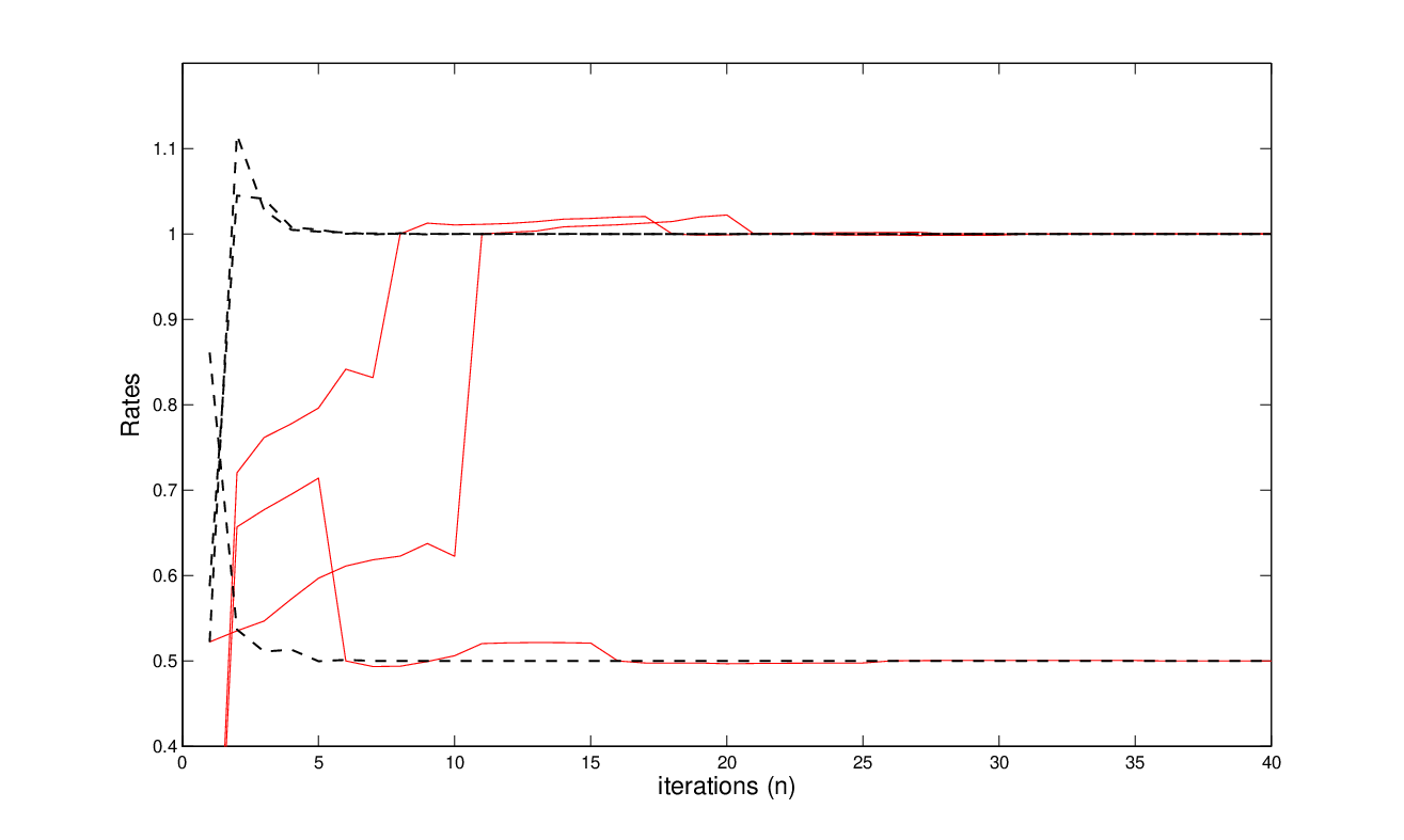
Numerical Example. As an example, in Figure 2, we compare the performance of the sequential and simultaneous IWFA, in terms of convergence speed. We consider a network composed of 10 links and we show the rate evolution of three of the links corresponding to the sequential IWFA and simultaneous IWFA as a function of the iteration index $n$ as defined in Algorithms 1 and 2. In Figure 2a) we consider a rate profile for the users with two different classes of service; whereas in Figure 2b) the same target rate for all the users is required. As expected, the sequential IWFA is slower than the simultaneous IWFA, especially if the number of active links $Q$ is large, since each user is forced to wait for all the other users scheduled before updating its power allocation.

5 Conclusions

In this paper we have considered the distributed power allocation in Gaussian parallel interference channels, subject to QoS constraints. More specifically, we have proposed a new game theoretic formulation of the power control problem, where each user aims at minimizing the transmit power while guaranteeing a prescribed information rate. We have provided sufficient conditions for the nonemptiness and the boundedness of the solution set of the Nash problem. These conditions suggest a simple admission control procedure to check the feasibility of any given users’ rate profile. As expected, there exists a trade-off between the performance achievable from each user (i.e., the achievable information rate) and the maximum level of interference that may be tolerated in the network. Under some additional conditions we have shown that the solution of the generalized Nash problem is unique and we have proved the convergence of two distributed algorithms: The sequential and the simultaneous IWFAs. Interestingly, although the rate constraints induce a coupling among the feasible strategies of the users, both algorithms are totally distributed, since each user, to compute the waterfilling solution, only needs to measure the noise-plus-interference power across the subchannels. Our results are thus appealing in all the practical distributed multipoint-to-multipoint systems, either wired or wireless, where centralized power control techniques are not allowed and QoS in terms of information rate must be guaranteed for each link.

One interesting direction that is worth of further investigations is the generalization of the proposed algorithms to the case of asynchronous transmission and totally asynchronous updates among the users, as did in [13] for the rate maximization game.

6 Appendices

Appendix A Proof of Theorem 5

We derive Theorem 5 as a corollary to the more general Theorem 23 below. In order to prove this theorem we need several preliminary concepts and results though, as given next.

A.1 Noiseless game

We rewrite first the KKT optimality conditions of the Nash problem (6) as a Mixed nonlinear Complementarity Problem (MNCP) [17, 32]. Denoting by $\mu_{q,k}$ the multipliers of the nonnegativity constraints and by $\lambda_{q}$ the multipliers of the rate constraint, the KKT conditions of problems (6) can be written as:

\begin{array}[]{ll}1-\mu_{q,k}-\lambda_{q}\dfrac{\left|H_{qq}(k)\right|^{2}}{\sigma_{{}_{q}}^{2}(k)+\sum_{\,r=1}^{Q}\left|H_{qr}(k)\right|^{2}p_{r}(k)}=0,&\quad\forall k\in\mathcal{N}\text{, }\forall q\in\Omega,\\ 0\,\leq\,p_{q}(k)\quad\perp\quad\mu_{q,k}\geq 0,&\quad\forall k\in\mathcal{N}\text{, }\forall q\in\Omega,\\ 0\,\leq\,\lambda_{q}\quad\quad\hskip 2.84544pt\perp\quad\,\,\,\,{\displaystyle\sum\limits_{k=1}^{N}}\log\left(1+\text{ }\dfrac{\left|H_{qq}(k)\right|^{2}p_{q}(k)}{\sigma_{{}_{q}}^{2}(k)+\sum_{\,r\neq q}\left|H_{qr}(k)\right|^{2}p_{r}(k)}\right)-R_{q}^{\star}\geq 0,&\quad\forall q\in\Omega,\end{array}

(31)

where $a\perp b$ means the two scalars (or vectors) $a$ and $b$ are orthogonal. Observe that each $\lambda_{q}>0;$ otherwise complementarity yields $\,p_{q}(k)=0$ for all $k\in\mathcal{N}$ , which contradicts the rate constraints.

Eliminating the multipliers $\{\mu_{q,k}\}$ corresponding to the nonnegativity constraints and making some obvious scaling, the KKT conditions in (31) are equivalent to the following MNCP:

\begin{array}[]{lll}0\,\leq\,p_{q}(k)&\perp&\sigma_{q}^{2}(k)+{\displaystyle\sum\limits_{r=1}^{Q}}\,|H_{qr}(k)|^{2}p_{r}(k)-|H_{qq}(k)|^{2}\,\lambda_{q}\,\geq\,0,\quad\forall k\in\mathcal{N}\text{, }\forall q\in\Omega.\\[5.0pt] 0\,\leq\,\lambda_{q},&&{\displaystyle\sum\limits_{k=1}^{N}}\,\log\left(1+\dfrac{|H_{qq}(k)|^{2}p_{q}(k)}{\sigma_{q}^{2}(k)+\sum_{r\neq q}|H_{qr}(k)|^{2}p_{r}(k)}\right)\,=\,R_{q}^{\star},\quad\forall q\in\Omega.\end{array}

(32)

To proceed further we introduce an additional game, which has the same structure of the game ${\mathscr{G}}$ , except for the players’ payoff functions, defined as in (2), but with $\sigma_{q}^{2}(k)=0$ for all $k\in\mathcal{N}$ and $q\in\Omega$ . We will refer to this game as the noiseless game. Although the noiseless game does not correspond to any realistic communication system, it will be shown to be instrumental in understanding the behavior of the original game ${\mathscr{G}}$ when all $\sigma_{q}^{2}(k)>0$ .

Note that the conditions $\sigma_{q}^{2}(k)>0$ ensure that all the users’ rates $R_{q}(\mathbf{p}_{q},\mathbf{p}_{-q})$ in (2) of the ${\mathscr{G}}$ in (6) are well-defined for all nonnegative $\mathbf{p}\triangleq(\mathbf{p}_{q})_{q=1}^{Q}$ , with $\mathbf{p}_{q}\triangleq(p_{q}(k))_{k=1}^{N}.$ Nevertheless, when $\sigma_{q}^{2}(k)=0$ , the players’ payoff functions⁶⁶ 6 With a slight abuse of notation, we use the same symbol to denote the payoff functions of the players in the game ${\mathscr{G}}$ in (6) and in the noiseless game. $R_{q}(\mathbf{p}_{q},\mathbf{p}_{-q})$ of the noiseless game still remain well-defined as long as ${\sum_{r=1}^{Q}}\,p_{\,r}(k)>0$ , provided that we allow for a rate equal to $\infty$ . Most importantly, the MNCP (32) is well defined for all nonnegative $\sigma_{q}^{2}(k)$ , including the case when $\sigma_{q}^{2}(k)=0$ for all $k\in\mathcal{N}$ and $q\in\Omega$ . The latter observation motivates the following definition.

Definition 20

A set of user powers $\mathbf{p}\triangleq(\mathbf{p}_{q})_{q=1}^{Q}$ , with $\mathbf{p}_{q}\triangleq(p_{q}(k))_{k=1}^{N},$ is said to be an almost GNE of the noiseless game if there exists a set of nonnegative scalars $\{v_{q}\}_{q=1}^{Q}$ such that

0\,\leq\,p_{\,q}(k)\,\perp\,{\sum_{r=1}^{Q}}\,|H_{qr}(k)|^{2}p_{r}(k)-|H_{qq}(k)|^{2}\,v_{q}\,\geq\,0,\quad\forall k\in\mathcal{N}\text{, }\forall q\in\Omega.

(33)

We call these solutions noiseless almost equilibria, and denote the set of noiseless equilibria by $\mathcal{NE}_{0}$ . $\Box$

The set $\mathcal{NE}_{0}$ of users’ noiseless almost equilibria constitutes a closed, albeit not necessarily convex, cone in the space of all users’ powers. A noteworthy point about such an almost equilibrium is the following simple property, which asserts that in the noiseless game, every subchannel will be used by at least one user.

Proposition 21

If $\mathbf{p}\in\mathcal{NE}_{0}$ , and $\mathbf{p}\neq\mathbf{0},$ then $\sum_{r=1}^{Q}p_{\,r}(k)>0$ for all $k\in\mathcal{N}$ .

Proof. Let ${\mathbf{p}}\in\mathcal{NE}_{0}$ be such that $p_{\,q_{0}}(k_{0})>0$ for some pair $(q_{0},k_{0})$ . By complementarity (see (33)), we have

|H_{q_{0}q_{0}}(k_{0})|^{2}\,v_{q_{0}}\,=\,{\sum_{r=1}^{Q}}\,|H_{q_{0}r}(k_{0})|^{2}\,p_{r}(k_{0})\,>\,0,

(34)

which implies

{\sum_{r=1}^{Q}}\,|H_{{q_{0}}r}(k)|^{2}\,p_{r}(k)\,\geq\,|H_{q_{0}q_{0}}(k)|^{2}\,v_{q_{0}}\,>\,0,\hskip 12.13678pt\forall k\in\mathcal{N},

(35)

since the $|H_{qr}(k)|^{2}$ are all positive. Equation (35) clearly implies:

{\sum_{r=1}^{Q}}\,p_{\,r}(k)\,>\,0,\hskip 12.13678pt\forall k\in\mathcal{N},

as claimed by the proposition.

A.2 The noiseless asymptotic cone

Another mathematical concept we need is that of asymptotic direction of a (nonconvex) set that we borrow from recession analysis [30].

Given the game ${\mathscr{G}}$ with rate profile ${\mathbf{R}}^{\star}\triangleq(R_{q}^{\star})_{q=1}^{Q}$ , it is possible that the sets of powers $\mathbf{p}$ that allow the user to achieve this rate be unbounded. In essence, the asymptotic consideration below aims at identifying such unbounded user powers. Specifically, we consider the following noisy nonconvex level set of users’ powers corresponding to ${\mathbf{R}}^{\star}$ :

\mathcal{P}^{\mbox{\boldmath{$\sigma$}}}({\mathbf{R}}^{\star})\,\equiv\,\left\{\,{\mathbf{p}}\,\geq\,0\,:\,{\sum_{k=1}^{N}}\,\log\left(1+\frac{|H_{qq}(k)|^{2}p_{q}(k)}{\sigma_{q}^{2}(k)+\sum_{r\neq q}|H_{qr}(k)|^{2}p_{r}(k)}\right)\,=\,R_{q}^{\star},\;\forall q\in\Omega\right\},\vskip 6.0pt plus 2.0pt minus 2.0pt

(36)

where $\mbox{\boldmath{$\sigma$}}\triangleq(\mbox{\boldmath{$\sigma$}}_{q})_{q=1}^{Q},$ with $\mbox{\boldmath{$\sigma$}}_{q}\triangleq(\sigma_{q}^{2}(k))_{k=1}^{N}.$ The asymptotic cone of $\mathcal{P}^{\mbox{\boldmath{$\sigma$}}}({\mathbf{R}}^{\star})$ , denoted by $\mathcal{P}_{\infty}^{\mbox{\boldmath{$\sigma$}}}({\mathbf{R}}^{\star})$ , is the cone (not necessarily convex) of directions ${\mathbf{d}}\triangleq{\left(\,\mathbf{d}_{q}\,\right)_{q=1}^{Q},}$ with ${\mathbf{d}}_{q}{\triangleq\left(\,d_{q}\,(k)\right)_{k=1}^{N},}$ such that

{\mathbf{d}}\,=\,{\lim_{\nu\rightarrow\infty}}\,{\dfrac{{\mathbf{p}}^{\nu}}{\tau_{\nu}}}

(37)

for some sequence of scalars ${\left\{\,\tau_{\nu}\,\right\}_{\nu=1}^{\infty}}$ tending to $\infty$ and some sequence of powers ${\left\{\,{\mathbf{p}}^{\nu}\,\right\}_{\nu=1}^{\infty}}$ such that ${\mathbf{p}}^{\nu}\in P^{\mbox{\boldmath{$\sigma$}}}({\mathbf{R}}^{\star})$ for all $\nu$ .

It is known [30, Proposition 2.1.2] that $\mathcal{P}^{\mbox{\boldmath{$\sigma$}}}({\mathbf{R}}^{\star})$ is bounded if and only if $\mathcal{P}_{\infty}^{\mbox{\boldmath{$\sigma$}}}({\mathbf{R}}^{\star})=\{\mathbf{0}\}$ . Whereas the individual sets $\mathcal{P}^{\mbox{\boldmath{$\sigma$}}}({\mathbf{R}}^{\star})$ are dependent on $\sigma_{q}^{2}(k)$ , it turns out that the asymptotic cones of all these sets are the same and equal to the following noiseless level set of users’ powers:

\mathcal{P}^{0}({\mathbf{R}}^{\star})\,\equiv\,\left\{\,{\mathbf{d}}\,{\triangleq}\,\left(\,\mathbf{d}_{\,q}\,\right)_{q=1}^{Q}\,\geq\,0\,:\,{\sum_{k:\sum_{r=1}^{Q}d_{r}(k)>0}}\,\log\left(\,1+{\frac{|H_{qq}(k)|^{2}\,d_{\,q}(k)}{{\sum_{r\neq q}}\,|H_{qr}(k)|^{2}\,d_{\,r}(k)}}\,\right)\,\leq\,R_{q}^{\star},\ \forall q\,\in\,\Omega\,\right\},

where by convention the vacuous summation is defined to be zero (i.e., by definition, $\mathcal{P}^{0}({\mathbf{R}}^{\star})$ contains the origin). The claim about the equality of $\mathcal{P}_{\infty}^{\mbox{\boldmath{$\sigma$}}}({\mathbf{R}}^{{}^{\star}})$ for a fixed ${\mathbf{R}}^{{}^{\star}}$ is formally stated and proved in the result below.

Proposition 22

For any $\mbox{\boldmath{$\sigma$}}>\mathbf{0}$ , $\mathcal{P}_{\infty}^{\mbox{\boldmath{$\sigma$}}}({\mathbf{R}}^{{}^{\star}})=\mathcal{P}^{0}({\mathbf{R}}^{{}^{\star}})$ .

Proof. Let $\mbox{\boldmath{$\sigma$}}>\mathbf{0}$ be arbitrary. Let ${\mathbf{d}}\in\mathcal{P}_{\infty}^{\mbox{\boldmath{$\sigma$}}}({\mathbf{R}}^{{}^{\star}})$ and $\{({\mathbf{p}}^{\nu},\tau_{\nu})\}$ be a sequence satisfying the definition of ${\mathbf{d}}$ in (37). For each $q\in\,\Omega$ and all $\nu$ , we have

\begin{array}[]{lll}R_{q}^{\star}&\geq&{\displaystyle\sum\limits_{k=1}^{N}}\,\log\left(\,1+{\dfrac{|H_{qq}(k)|^{2}\,p_{q}^{\nu}(k)}{\sigma_{q}^{2}(k)+{\displaystyle\sum_{r\neq q}}\,|H_{qr}(k)|^{2}\,p_{r}^{\nu}(k)}}\,\right)\\[36.135pt] &\geq&{\displaystyle\sum\limits_{k:\sum_{r=1}^{Q}d_{r}(k)>0}}\,\log\left(\,1+{\dfrac{|H_{qq}(k)|^{2}\,p_{q}^{\nu}(k)}{\sigma_{q}^{2}(k)+{\displaystyle\sum_{r\neq q}}\,|H_{qr}(k)|^{2}\,p_{r}^{\nu}(k)}}\,\right)\\[36.135pt] &=&{\displaystyle\sum\limits_{k:\sum_{r=1}^{Q}d_{r}(k)>0}}\log\left(\,1+{\dfrac{|H_{qq}(k)|^{2}\,{\dfrac{p_{q}^{\nu}(k)}{\tau_{\nu}}}}{{\dfrac{\sigma_{q}^{2}(k)}{\tau_{\nu}}}+{\displaystyle\sum_{r\neq q}}|H_{qr}(k)|^{2}{\dfrac{p_{r}^{\nu}(k)}{\tau_{\nu}}}}}\,\right).\end{array}

(38)

Taking the limit $\nu\rightarrow\infty$ establishes the inclusion $\mathcal{P}_{\infty}^{\mbox{\boldmath{$\sigma$}}}({\mathbf{R}}^{\star})\subseteq\mathcal{P}^{0}({\mathbf{R}}^{\star})$ .

Conversely, it is clear that $\mathbf{0}\in\mathcal{P}^{\mbox{\boldmath{$\sigma$}}}({\mathbf{R}}^{\star})$ . Let ${\mathbf{d}}$ be a nonzero vector in $\mathcal{P}^{0}({\mathbf{R}}^{\star})$ . For any scalar $\theta>0$ , we have, for all $q\in\Omega,$

\begin{array}[]{l}{\displaystyle\sum\limits_{k=1}^{N}}\,\log\left(\,1+{\dfrac{\theta\,|H_{qq}(k)|^{2}\,\,d_{\,q}(k)}{\sigma_{q}^{2}(k)+\theta\,{\sum_{r\neq q}}\,|H_{qr}(k)|^{2}\,d_{\,r}(k)}}\,\right)\\ \hskip 142.26378pt={\displaystyle\sum\limits_{k:\sum_{r=1}^{Q}d_{r}(k)>0}}\log\left(\,1+{\dfrac{\theta\,|H_{qq}(k)|^{2}\,d_{\,q}(k)}{\sigma_{q}^{2}(k)+\theta\,{\sum_{r\neq q}}\,|H_{qr}(k)|^{2}\,d_{\,r}(k)}}\,\right)\\ \hskip 142.26378pt\leq{\displaystyle\sum\limits_{k:\sum_{r=1}^{Q}d_{r}(k)>0}}\,\log\left(\,1+{\dfrac{|H_{qq}(k)|^{2}\,d_{\,q}(k)}{{\sum_{r\neq q}}\,|H_{qr}(k)|^{2}\,d_{\,r}(k)}}\,\right).\end{array}

(39)

Hence $\theta{\mathbf{d}}\in\mathcal{P}^{\mbox{\boldmath{$\sigma$}}}({\mathbf{R}}^{\star})$ for all $\theta>0$ . It follows that ${\mathbf{d}}\in\mathcal{P}_{\infty}^{\mbox{\boldmath{$\sigma$}}}({\mathbf{R}}^{\star})$ .

We are now ready to introduce the key object in our proof of Theorem 23, the cone $\mathcal{NE}_{0}\cap\mathcal{P}^{0}({\mathbf{R}}^{\mathbf{\star}})$ , which by Proposition 22, is equal to $\{\mathbf{0}\}\cup\widehat{\mathcal{NE}}_{0}({\mathbf{R}}^{\star})$ , where

\begin{array}[]{lll}\widehat{\mathcal{NE}}_{0}({\mathbf{R}}^{\star})&\triangleq&\left\{\,{\mathbf{d}}\,\in\,\mathcal{NE}_{0}\,\setminus\,\{\,\mathbf{0}\,\}\,:\,{\displaystyle\sum\limits_{k=1}^{N}}\,\log\left(\,1+{\dfrac{|H_{qq}(k)|^{2}\,d_{\,q}(k)}{{\sum_{r\neq q}}\,|H_{qr}(k)|^{2}\,d_{\,r}(k)}}\,\right)\,\leq\,R_{q}^{\star},\ \forall q\,\in\Omega\right\}\\[28.90755pt] &=&\mathcal{NE}_{0}\,\cap\,\mathcal{P}^{0}({\mathbf{R}}^{\star})\,\setminus\,\{\,\mathbf{0}\,\}.\end{array}

(40)

Notice that ${\mathbf{d}}\in\widehat{\mathcal{NE}}_{0}({\mathbf{R}}^{\star})$ implies ${\sum_{r\neq q}|H_{qr}(k)|^{2}d_{\,r}(k)>0}$ for all $q\,\in\Omega$ and all $k\,\in\mathcal{N}$ .

A.3 Existence results

With the above preparation, we are ready to present our main existence theorem. The emptiness of the set $\widehat{\mathcal{NE}}_{0}({\mathbf{R}}^{\star})$ defined in (40) turns out to provide a sufficient condition for the MNCP (32) to have a nonempty bounded solution set.

Theorem 23

Given the game ${\mathscr{G}}$ with rate profile $\mathbf{R}^{\star}\triangleq(R_{q}^{\star})_{q=1}^{Q}>\mathbf{0}$ , if $\widehat{\mathcal{NE}}_{0}(\mathbf{R}^{\star})=\emptyset$ , then the game has a nonempty and bounded solution set, for all $\mbox{\boldmath{$\sigma$}}>\mathbf{0}$ .

Proof. We first note that the KKT conditions of the Nash problem defined in (6) are equivalent to the following nonlinear complementarity problem (NCP) (see (31) and comments thereafter)

\begin{array}[]{lll}0\,\leq\,p_{\,q}(k)&\perp&\sigma_{q}^{2}(k)+{\displaystyle\sum\limits_{r=1}^{Q}}\,|H_{qr}(k)|^{2}\,p_{\,r}(k)-|H_{qq}(k)|^{2}\,\lambda_{q}\,\geq\,0,\quad\forall k\in\mathcal{N}\text{, }\forall q\in\Omega,\\[5.0pt] 0\,\leq\,\lambda_{q}&\perp&{\displaystyle\sum\limits_{k=1}^{N}}\,\log\left(\,1+{\dfrac{|H_{qq}(k)|^{2}\,p_{\,q}(k)}{\sigma_{q}^{2}(k)+{\sum_{r\neq q}}\,|H_{qr}(k)|^{2}\,p_{\,r}(k)}}\,\right)-R_{q}^{\star}\,\geq\,0,\quad\forall q\in\Omega,\end{array}

(41)

In turn, to show that (41) has a solution, it suffices to prove that the solutions of the augmented NCP

\begin{array}[]{lll}0\,\leq\,p_{\,q}(k)&\perp&\sigma_{q}^{2}(k)+{\displaystyle\sum\limits_{r=1}^{Q}}\,|H_{qr}(k)|^{2}\,p_{\,r}(k)-|H_{qq}(k)|^{2}\lambda_{q}+\tau\,p_{\,q}(k)\,\geq\,0,\quad\forall k\in\mathcal{N}\text{, }\forall q\in\Omega,\\[5.0pt] 0\,\leq\,\lambda_{q}&\perp&{\displaystyle\sum\limits_{k=1}^{N}}\,\log\left(\,1+{\dfrac{|H_{qq}(k)|^{2}p_{\,q}(k)}{\sigma_{q}^{2}(k)+{\displaystyle{\sum_{r\neq q}}\,|H_{qr}(k)|^{2}p_{\,r}(k)}}}\,\right)-R_{q}^{\star}+\tau\,\lambda_{q}\,\geq\,0,\quad\forall q\in\Omega,\end{array}

for all $\tau>0$ are bounded [17, Theorem $2.6.1$ ].

We show the latter boundedness property by contradiction. Assume that for some sequence of positive scalars $\{\tau_{\nu}\}$ , a sequence of solutions $\{({\mathbf{p}}^{\nu},\tau_{\nu})\}$ exists such that each pair $({\mathbf{p}}^{\nu},\tau_{\nu})$ satisfies:

\begin{array}[]{lll}0\,\leq\,p_{q}^{\nu}(k)&\perp&\sigma_{q}^{2}(k)+{\displaystyle\sum\limits_{r=1}^{Q}}\,|H_{qr}(k)|^{2}p_{r}^{\nu}(k)-|H_{qq}(k)|^{2}\,\lambda_{q}^{\nu}+\tau_{\nu}\,p_{q}^{\nu}(k)\,\geq\,0\quad\forall k\in\mathcal{N}\text{, }\forall q\in\Omega,\\[5.0pt] 0\,\leq\,\lambda_{q}^{\nu}&\perp&{\displaystyle{\displaystyle\sum\limits_{k=1}^{N}}\,\log\left(\,1+{\dfrac{|H_{qq}(k)|^{2}\,\,p_{q}^{\nu}(k)}{\sigma_{q}^{2}(k)+{\sum_{r\neq q}}\,|H_{qr}(k)|^{2}\,\,p_{r}^{\nu}(k)}}\,\right)-R_{q}^{\star}+\tau_{\nu}\,\lambda_{q}^{\nu}\,\geq\,0,\quad\forall q\in\Omega,}\end{array}

(42)

and that

\lim_{\nu\rightarrow\infty}\,\left[\,\|\,{\mathbf{p}}^{\nu}\,\|+{\sum_{q=1}^{Q}}\,\lambda_{q}^{\nu}\,\right]\,=\,\infty.

(43)

From (42), it is clear that $\lambda_{q}^{\nu}>0$ for all $\nu$ and $q$ . In fact, if a $\lambda_{q}^{\nu}=0$ , then by the first complementarity condition, $p_{q}^{\nu}(k)=0$ for all $k$ , which is not possible by the last inequality in (42).

Thus, it follows from the second complementarity condition that

{\sum_{k=1}^{N}}\,\log\left(\,1+{\frac{|H_{qq}(k)|^{2}\,p_{q}^{\nu}(k)}{\sigma_{q}^{2}(k)+{\displaystyle\sum_{r\neq q}}\,|H_{qr}(k)|^{2}p_{r}^{\nu}(k)}}\,\right)-R_{q}^{\star}+\tau_{\nu}\,\lambda_{q}^{\nu}\,=\,0,

(44)

which implies that the sequence $\{\tau_{\nu}\lambda_{q}^{\nu}\}$ is bounded for each $q\in\Omega$ . We claim that ${\lim_{\nu\rightarrow\infty}\tau_{\nu}=0}$ . Otherwise, for some subsequence $\{\tau_{\nu}:\nu\in\kappa\}$ , where $\kappa$ is an infinite index set, we have ${\liminf_{\nu(\in\kappa)\rightarrow\infty}\tau_{\nu}>0}$ . Thus, the subsequence $\{\lambda_{q}^{\nu}:\nu\in\kappa\}$ is bounded for all $q\in\Omega$ . The first complementarity condition in (42) then implies that $\{p_{q}^{\nu}(k):\nu\in\kappa\}$ is bounded for all $q\in\Omega$ and $k\in\mathcal{N}$ . This is a contradiction to (43). Therefore, the sequence $\{\tau_{\nu}\}\downarrow 0$ .

Consider now the normalized sequence $\{{\mathbf{p}}^{\nu}/\|{\mathbf{p}}^{\nu}\|\}$ , which must have at least one accumulation point; moreover, any such point must be nonzero. Let ${\mathbf{d}}^{\infty}$ be any such point. It is not difficult to show that ${\mathbf{d}}^{\infty}$ is a nonzero almost noiseless equilibrium. Moreover, from the inequality:

{\sum_{k=1}^{N}}\,\log\left(\,1+{\frac{|H_{qq}(k)|^{2}\,p_{q}^{\nu}(k)}{\sigma_{q}^{2}(k)+{\sum_{r\neq q}}\,|H_{qr}(k)|^{2}\,p_{r}^{\nu}(k)}}\,\right)-R_{q}^{\star}\,\leq\,0,

(45)

which is implied by (44), it is equally easy to show that ${\mathbf{d}}^{\infty}\in\mathcal{P}^{0}({\mathbf{R}}^{\star})$ . Therefore, ${\mathbf{d}}^{\infty}$ is an element of $\widehat{\mathcal{NE}}_{0}({\mathbf{R}}^{\star})$ , which is a contradiction. This completes the proof of the existence of a solution to the problem (32). The boundedness of such solutions can be proved in a similar way via contradiction and by the same normalization argument. The details are not repeated.

Roughly speaking, the key condition $\widehat{\mathcal{NE}}_{0}({\mathbf{R}}^{\star})=\emptyset$ in the previous theorem is just the mathematical requirement that if the power ${\mathbf{p}}$ goes to infinity staying feasible, the system cannot approach a (noiseless) equilibrium. As such the previous theorem is rather natural, although it does not provide an effective way of checking the existence and boundedness of the solutions. To this end, however, we can now easily derive Theorem 5 from Theorem 23.

A.4 Proof of Theorem 5

In order to prove Theorem 5 we introduce a simple polyhedral set that will turn out to be a subset of $P^{\mbox{\boldmath{$\sigma$}}}({\mathbf{R^{\star}}})$ .

{\normalsize P}_{\infty}({\mathbf{R^{\star}}})\,\triangleq\,{\prod_{k=1}^{N}}\,\left\{\,\mathbf{r}(k)\,\in\mathbb{R}_{+}^{\,Q}\,:\,\mathbf{Z}_{k}({\mathbf{R^{\star}}})\mathbf{r}(k)\,\leq\,\mathbf{0}\,\right\},

(46)

which is independent of the $\sigma$ and where, we recall, the matrices $\mathbf{Z}_{k}({\mathbf{R^{\star}}})$ are defined by (11). The key property for the existence Theorem 5 is stated in the following proposition.

Proposition 24

$\widehat{\mathcal{NE}}_{0}(\mathbf{R^{\star}})\subseteq P_{\infty}(\mathbf{R^{\star}})\cap(\mathcal{NE}_{0}\setminus\{\mathbf{0}\})$ .

Proof. It suffices to note the following string of implications:

\begin{array}[]{lll}{\mathbf{p}}\,\in\,\widehat{\mathcal{NE}}_{0}({\mathbf{R^{\star}}})&\Rightarrow&\log\left(\,1+{\dfrac{|H_{qq}(k)|^{2}\,p_{\,q}(k)}{{\sum_{r\neq q}}\,|H_{qr}(k)|^{2}\,p_{\,r}(k)}}\,\right)\,\leq\,R_{q}^{\star},\hskip 12.13678pt\forall\,q\,\in\Omega,\\ &\Leftrightarrow&|H_{qq}(k)|^{2}\,p_{\,q}(k)\,\leq\,(\,e^{R_{q}^{\star}}-1\,)\,{\displaystyle\sum_{r\neq q}}\,|H_{qr}(k)|^{2}\,p_{\,r}(k),\hskip 12.18237pt\forall\,q\,\in\Omega,\\[10.0pt] &\Leftrightarrow&{\mathbf{p}}\,\in\,P_{\infty}({\mathbf{R^{\star}}}).\end{array}

(47)

where the middle equivalence is by simple exponentiation.

It is known that, since each matrix $\mathbf{Z}_{k}({\mathbf{R}}^{\star})$ is a Z-matrix, if each matrix $\mathbf{Z}_{k}({\mathbf{R}}^{\star})$ is also a P-matrix, then a positive vector $\mathbf{s}(k)\triangleq(s_{q}(k))_{q=1}^{Q}$ exists such that $\mathbf{s}^{T}(k)\mathbf{Z}_{k}({\mathbf{R}}^{\star})>\mathbf{0}$ [32, Theorem $3.3.4$ ]. But this implies that $P_{\infty}({\mathbf{R}}^{\star})=\{\mathbf{0}\}$ , and thus $\widehat{\mathcal{NE}}_{0}({\mathbf{R}}^{\star})=$ $\emptyset$ . The first assertion of Theorem 5 then follows immediately from Theorem 23. It remains to establish the bound on the $\mathbf{p}(k)=(p_{q}(k))_{q=1}^{Q}$ . This follows easily from the following two facts: 1) any solution ${\mathbf{p}}$ of (32) must belong to the set $P^{\mbox{\boldmath{$\sigma$}}}({\mathbf{R}}^{\star})$ ; 2) a Z-matrix that is also a P-matrix must have a nonnegative inverse.

Appendix B Proof of Corollary 6

Consider the matrix ${\mathbf{Z}}^{\max}({\mathbf{R^{\star}}})$ defined by (13) in Corollary 6, and assume it is a P-matrix. Set $\mathbf{D}(k)\triangleq{\mbox{ Diag}\left(|H_{qq}(k)|^{2}\right)_{q=1}^{Q}}$ . The first assertion in the Corollary is immediate because

\mathbf{Z}_{k}({\mathbf{R}}^{\star})\geq{\mathbf{Z}}^{\max}({\mathbf{R}}^{\star})\mathbf{D}(k),\quad\forall k\in\mathcal{N}\text{,}

(48)

where the inequality is intended component-wise. Therefore, since all the matrices involved are Z-matrices, from the assumption on ${\mathbf{Z}}^{\max}({\mathbf{R}}^{\star}),$ it follows that all the $\mathbf{Z}_{k}({\mathbf{R}}^{\star})$ are also P-matrices.⁷⁷ 7 The last statement can be easily proved using [32, Lemma 5.3.14]. Lets now prove the bounds (15). Note first that

\left(\begin{array}[]{c}\sigma_{1}^{2}(k)\,(\,e^{R_{1}^{\ast}}-1\,)\\[5.0pt] \vdots\\[5.0pt] \sigma_{Q}^{2}(k)\,(\,e^{R_{Q}^{\ast}}-1\,)\end{array}\right)\,\leq\,\left[\,{\max_{r\in\Omega}}\,\sigma_{r}^{2}(k)\,\right]\,(\,e^{\mathbf{R}{\mathbf{{}^{\ast}}}}-\mbox{\boldmath{$1$}}\,),\quad\forall k\in\mathcal{N}\text{.}

(49)

Furthermore we recall that, by (48), we have $\left[\mathbf{Z}_{k}({\mathbf{R}}^{\star})\right]^{-1}\leq\left[{\mathbf{Z}}^{\max}({\mathbf{R}}^{\star})\mathbf{D}(k)\right]^{-1}$ [32], and also that the inverse of a matrix that is P and Z is nonnegative [32, Theorem $3.11.10$ ]. From all these facts, and recalling (12), the following chain of inequalities easily follows for every $k\in\mathcal{N}$ :

	$\displaystyle\mathbf{D}(k)\,\left(\begin{array}[]{c}\overline{p}_{1}(k)\\[5.0pt] \vdots\\[5.0pt] \overline{p}_{Q}(k)\end{array}\right)$	$\displaystyle\leq\mathbf{D}(k)\,[\,\mathbf{Z}_{k}({\mathbf{R}}^{\star})\,]^{-1}\left(\begin{array}[]{c}\sigma_{1}^{2}(k)\,(\,e^{R_{1}^{\star}}-1\,)\\[5.0pt] \vdots\\[5.0pt] \sigma_{Q}^{2}(k)\,(\,e^{R_{Q}^{\star}}-1\,)\end{array}\right)$
		$\displaystyle\leq\left[{\max_{r\in\Omega}}\,\sigma_{r}^{2}(k)\,\right]\,\left[{\mathbf{Z}}^{\max}({\mathbf{R}}^{\star})\right]^{-1}\,(\,e^{\mathbf{R}{\mathbf{{}^{\star}}}}-\mbox{\boldmath{$1$}}\,),$		(56)

which provides the desired bound (15).

Appendix C Proof of Proposition 11

We prove that the following three statements are equivalent for game $\mathscr{G}$ when $N=1$ :

(a): The game has a nonempty solution set;
(b): The matrix $\mathbf{Z}(\mathbf{R}^{\star})$ is a P-matrix;
(c): $\widehat{\mathcal{NE}}_{0}(\mathbf{R}^{\star})=\emptyset$ .

(a) $\Rightarrow$ (b). Since $N=1$ , any solution of (32) satisfies the equations

\log\left(\,1+{\dfrac{|H_{qq}(k)|^{2}p_{\,q}(k)}{\sigma_{q}^{2}(k)+{\displaystyle{\sum_{r\neq q}}\,|H_{qr}(k)|^{2}p_{\,r}(k)}}}\,\right)\,=\,R_{q}^{\star},\quad\forall q\in\Omega,

which are easily seen to be equivalent to (26). Since the right-hand constants in (26) are positive, it follows that a vector $\mathbf{r}^{\star}\triangleq(r_{q}^{\star})_{q=1}^{Q}\geq\mathbf{0}$ , which is the solution of (32) with $N=1$ , exists satisfying $\mathbf{Z}(\mathbf{R}^{\star})\mathbf{r}^{\star}>0$ . Hence (b) follows [32, Theorem 3.3.4], [31, Theorem 6.2.3]. The implications (b) $\Rightarrow$ (c) $\Rightarrow$ (a) come directly from the more general case $N\geq 1$ . Hence (a), (b), and (c) are equivalent.

It remains to establish the assertion about the uniqueness of the solution. But this is clear because any one of the three statements (a), (b), or (c) implies that the matrix $\mathbf{Z}(\mathbf{R}^{\star})$ is a P-matrix, thus nonsingular [31, Theorem 6.2.3]; and hence the system of linear equations (26) has a unique solution.

Appendix D Proof of Theorem 9

The study of the uniqueness of the solution of the GNEP is complicated by the presence of a coupling among the feasible strategy sets of the users, due to the rate constraints. To overcome this difficulty we first introduce a change of variables of the game ${\mathscr{G}}$ , from the power variables $p_{q}(k)$ to a set of rate variables, in order to obtain an equivalent formulation of the original generalized Nash problem as a Variational Inequality (VI) problem, defined on the Cartesian product of the users’ rate admissible sets. Then, building on this VI formulation, we derive sufficient conditions for the uniqueness of the GNE of the original game. It is important to remark that our VI formulation of the game ${\mathscr{G}}$ differs from that of [11]. In fact, in [11] the rate maximization game was formulated as an Affine VI defined on the Cartesian product of the users’ power sets [11, Proposition $2$ ]. Our VI instead, is defined by a nonlinear function, which significantly complicates the uniqueness analysis, as detailed next.

D.1 VI formulation

Hereafter we assume that conditions of Theorem 5 are satisfied, so that a GNE of the game ${\mathscr{G}}$ is guaranteed to exist.

Given the game ${\mathscr{G}}$ we introduce the following change of variables:

r_{q}(k)\,\triangleq\,\log\left(\,1+{\frac{|H_{qq}(k)|^{2}\,p_{q}(k)}{\sigma_{q}^{2}(k)+{\sum_{r\neq q}}\,|H_{qr}(k)|^{2}\,p_{r}(k)}}\,\right),\hskip 12.27356ptk\in\mathcal{N}\text{, }q\in\Omega,

(57)

with $r_{q}(k)$ satisfying the constraints

r_{q}(k)\geq 0,\text{ \ }\forall k\in\mathcal{N}\text{, }\forall q\in\Omega,\quad\text{and}\quad{\sum_{k=1}^{N}r_{q}(k)=R_{q}^{\star}},\text{ \ }\forall q\in\Omega.

(58)

Observe that each $r_{q}(k)=0$ if and only if $p_{q}(k)=0.$ Given $\mathbf{r}(k)\triangleq(r_{q}(k))_{q=1}^{Q},$ let us define the Z-matrix $\mathbf{Z}_{k}(\mathbf{r}(k))\in\mathbb{R}^{Q\times Q}$ as $:$

\mathbf{Z}_{k}(\mathbf{r}(k))\,\triangleq\,\,\left[\begin{array}[]{cccc}|H_{11}(k)|^{2}&-(e^{r_{1}(k)}-1)\,|H_{12}(k)|^{2}&\cdots&-(e^{r_{1}(k)}-1)\,|H_{1Q}(k)|^{2}\\[7.0pt] -(e^{r_{2}(k)}-1)\,|H_{21}(k)|^{2}&|H_{22}(k)|^{2}&\cdots&-(e^{r_{2}(k)}-1)\,|H_{2Q}(k)|^{2}\\[7.0pt] \vdots&\vdots&\ddots&\vdots\\[7.0pt] -(e^{r_{Q}(k)}-1)\,|H_{Q1}(k)|^{2}&-(e^{r_{Q}(k)}-1)\,|H_{Q2}(k)|^{2}&\cdots&|H_{QQ}(k)|^{2}\end{array}\right]\,.

(59)

From (58), we have $\mathbf{Z}_{k}(\mathbf{r}(k))\,\geq\mathbf{Z}_{k}(\mathbf{R}^{\star})\,$ for all $k\in\mathcal{N}$ , where $\mathbf{Z}_{k}(\mathbf{R}^{\star})$ is defined in (11). It follows that each $\mathbf{Z}_{k}(\mathbf{r}(k))$ is a P-matrix.

According to (57), the users’ powers $\mathbf{p}(k)\triangleq(p_{q}(k))_{q=1}^{Q}$ are related to the rates $\mathbf{r}(k)$ by the following function

\left(\begin{array}[]{c}p_{1}(k)\\[3.0pt] \vdots\\[3.0pt] p_{Q}(k)\end{array}\right)\,=\mathbf{\boldsymbol{\phi}}(k,\mathbf{r}(k))\triangleq\,\left(\,\mathbf{Z}_{k}(\mathbf{r}(k))\right)^{-1}\left(\begin{array}[]{c}\sigma_{1}^{2}(k)\,(\,e^{r_{1}(k)}-1\,)\\[3.0pt] \vdots\\[3.0pt] \sigma_{Q}^{2}(k)\,(\,e^{r_{Q}(k)}-1\,)\end{array}\right)\,,\quad k\in\mathcal{N}\text{.}

(60)

Observe that $\left(\,\mathbf{Z}_{k}(\mathbf{r}(k))\right)^{-1}$ is well-defined, since $\,\mathbf{Z}_{k}(\mathbf{r}(k))$ is a P-matrix [32, Theorem 3.11.10].

Using (58) and (60), and the fact that each $p_{q}(k)=0$ if and only if $r_{q}(k)=0$ , the KKT conditions of the Nash problem (6) can be rewritten as (see (32)):

\begin{array}[]{lll}0\,\leq\,r_{q}(k)&\perp&\sigma_{q}^{2}(k)+{\sum\limits_{r=1}^{Q}}\,|H_{qr}(k)|^{2}\,\phi_{r}(k,\mathbf{r}(k))-|H_{qq}(k)|^{2}\,\lambda_{q}\,\geq\,0,\quad\forall k\in\mathcal{N}\text{, }\forall q\in\Omega\\[5.0pt] 0\,\leq\,\lambda_{q},&&{\displaystyle\sum\limits_{k=1}^{N}}\,r_{q}(k)\,={R_{q}^{\star}},\quad\forall q\in\Omega\end{array}

(61)

where $\phi_{r}(k,\mathbf{r}(k))$ denotes the $r$ -th component of $\mathbf{\boldsymbol{\phi}}(k,\mathbf{r}(k)),$ defined in (60). It is easy to see that (61) is equivalent to (note that as usual $\lambda_{q}>0$ for any solution of (61)), $\forall k\in\mathcal{N}\text{, }\forall q\in\Omega$ ,

\begin{array}[]{lll}0\,\leq\,r_{q}(k)&\perp&\log\left(\sigma_{q}^{2}(k)+{\sum\limits_{r=1}^{Q}}\,|H_{qr}(k)|^{2}\,\phi_{r}(k,\mathbf{r}(k))\right)-\log\left(|H_{qq}(k)|^{2}\right)+\nu_{q}\,\geq\,0,\\[5.0pt] \nu_{q}\text{ free,}&&{\displaystyle\sum\limits_{k=1}^{N}}\,r_{q}(k)\,={R_{q}^{\star}},\end{array}

(62)

Let us define

\begin{array}[]{l}\Phi_{q}(k,\mathbf{r}(k))\triangleq\log\left(\sigma_{q}^{2}(k)+{\sum\limits_{r=1}^{Q}}\,|H_{qr}(k)|^{2}\,\phi_{r}(k,\mathbf{r}(k))\right)-\log\left(|H_{qq}(k)|^{2}\right),\quad k\in\mathcal{N}\text{, }q\in\Omega.\\ \mathbf{\Phi}_{q}({\mathbf{r}})\triangleq(\Phi_{q}(k,\mathbf{r}(k)))_{k=1}^{N},\quad\mathbf{\Phi}({\mathbf{r}})\triangleq(\mathbf{\Phi}_{q}({\mathbf{r}}))_{q=1}^{Q},\quad{\mathbf{r}}\triangleq(\mathbf{r}_{q})_{q=1}^{Q},\end{array}

(63)

with $\mathbf{r}_{q}\triangleq(r_{q}(k))_{k=1}^{N}$ . Observe that each $\Phi_{q}(k,\mathbf{r}(k))$ in (63) is a well-defined continuously differentiable function on the rectangular box ${[\mathbf{0},\mathbf{R}^{\star}]\triangleq\prod_{q=1}^{Q}\,[0,}R_{q}^{\star}{]\subset\mathbb{R}^{Q}}$ ; thus $\mathbf{\Phi}$ in (63) is a well-defined continuously differentiable function on ${[\mathbf{0},\mathbf{R}^{\star}]}^{N}$ .

Using (63), one can see that (62) are the KKT conditions of the VI $(U,\mathbf{\Phi})$ [17, Proposition $1.3.4$ ], where $U$ is the Cartesian product of users’ rate sets, defined as

U\,\equiv\,\prod_{q=1}^{Q}\,U_{q},\hskip 12.31915pt\mbox{where}\hskip 12.31915ptU_{q}\,\triangleq\,\left\{\,\mathbf{r}_{q}\,\in\,{\mathbb{R}_{+}^{N}}\,:{\sum_{k=1}^{N}}\,r_{q}(k)\,=R_{q}^{\star}\,\right\},

(64)

and $\mathbf{\Phi}$ is the continuously differentiable function on ${[\mathbf{0},\mathbf{R}^{\star}]}^{N}$ defined in (63).

By definition, it follows that a tuple $\mathbf{r}^{\star}\triangleq(\mathbf{r}_{q}^{\star})_{q=1}^{Q}$ is a solution of the VI $(U,\mathbf{\Phi})$ defined above if and only if, for all $\mathbf{r}_{q}\in U_{q}$ and $q\in\Omega,$

{\sum_{k=1}^{N}}\,\left(\,r_{q}(k)-r_{q}^{\star}(k)\,\right)\,\left[\,\log\left(\sigma_{q}^{2}(k)+{\sum\limits_{r=1}^{Q}}\,|H_{qr}(k)|^{2}\,\phi_{r}(k,\mathbf{r}_{k}^{\star})\right)-\log\left(|H_{qq}(k)|^{2}\,\right)\,\right]\,\geq\,0.

(65)

We rewrite now condition (65) in a more useful form. To this end, let introduce

\tau_{q}(k,\mathbf{p}(k))\,\triangleq\,\sigma_{q}^{2}(k)+{\sum_{r\neq q}}\,|H_{qr}(k)|^{2}\,p_{r}(k),\quad k\in\mathcal{N}\text{, }q\in\Omega,

(66)

with $\mathbf{p}(k)\,\triangleq\,\,\left(\,p_{q}(k)\right)_{q=1}^{Q}.$ For any solution $\mathbf{p}^{\star}=(\mathbf{p}^{\star}(k))_{k=1}^{N}$ of (31) (i.e., any GNE of the game ${\mathscr{G}}$ we have $\mathbf{p}^{\star}\leq\mathbf{\bar{p}}$ , where $\mathbf{\bar{p}}=(\mathbf{\bar{p}}(k))_{k=1}^{N},$ with $\mathbf{\bar{p}}(k)=(\bar{p}_{r}(k))_{r=1}^{Q}$ and $\bar{p}_{r}(k)$ defined in (12). It follows that

\sigma_{q}^{2}(k)\leq\tau_{q}(k,\mathbf{p}^{\star}(k))\,\leq\,\bar{\tau}_{q}(k)\,\triangleq\,\sigma_{q}^{2}(k)+{\sum_{r\neq q}}\,|H_{qr}(k)|^{2}\,\bar{p}_{r}(k),\quad\forall k\in\mathcal{N}\text{, }\forall q\in\Omega.

(67)

Using (66), we can write

\log\left(\sigma_{q}^{2}(k)+{\sum\limits_{r\neq q}^{Q}}\,|H_{qr}(k)|^{2}\,p_{r}(k)+|H_{qq}(k)|^{2}\,p_{q}(k)\right)=r_{q}(k)+\log\left(\tau_{q}(k,\mathbf{p}(k))\,\right),

(68)

so that condition (65) becomes

{\sum_{k=1}^{N}}\,\left(\,r_{q}(k)-r_{q}^{\star}(k)\,\right)\,\left(\,\log\left(\tau_{q}(k,\mathbf{p}^{\star}(k))\,\right)-\log\left(|H_{qq}(k)|^{2}\right)+r_{q}^{\star}(k)\,\right)\,\geq\,0,\hskip 12.41162pt\forall\,\mathbf{r}_{q}\in U_{q},\quad\forall q\in\Omega,

(69)

where $\tau_{q}(k,\mathbf{p}^{\star}(k))$ is defined in (66) and $\mathbf{p}^{\star}(k)\triangleq(p_{q}^{\star}(k))_{q=1}^{Q},$ with each $p_{q}^{\star}(k)=\phi_{q}(k,\mathbf{r}^{\star}(k)),$ and $\phi_{q}(\mathbf{\cdot})$ given in (60). Condition (69) will be instrumental for the study of the uniqueness of the GNE, as shown next.

D.2 Uniqueness analysis

Building on (69), we derive now sufficient conditions for the uniqueness of the GNE of the game ${\mathscr{G}}$ . Let $\widehat{{\mathbf{p}}}^{\,(\nu)}\triangleq(\widehat{\mathbf{p}}_{q}^{(\nu)})_{q=1}^{Q},$ for $\nu=1,2,$ be any two solutions of the Nash problem in (6). Given $\nu=1,2$ , $k\in\mathcal{N},$ and $q\in\Omega,$ let us define

\widehat{r}_{q}^{(\nu)}(k)\,\triangleq\log\left(\,1+{\frac{|H_{qq}(k)|^{2}\,\widehat{p}_{q}^{(\nu)}(k)}{\sigma_{q}^{2}(k)+{\sum_{r\neq q}}\,|H_{qr}(k)|^{2}\,\widehat{p}_{r}^{(\nu)}(k)}}\,\right),\hskip 12.64563pt\text{and}\hskip 12.6936pt\widehat{\tau}_{q}^{(\nu)}(k)\triangleq\tau_{q}(k,\widehat{\mathbf{p}}^{(\nu)}(k)).\quad

(70)

Adding the following two inequalities, which are obtained from the characterization (69) of a solution to the VI $(U,\mathbf{\Phi})$ :

{\sum_{k=1}^{N}}\,\left(\,\widehat{r}_{q}^{\,(2)}(k)-\widehat{r}_{q}^{\,(1)}(k)\,\right)\,\left(\,-\log\left(|H_{qq}(k)|^{2}\right)+\log(\widehat{\tau}_{q}^{\,(1)}(k))+\widehat{r}_{q}^{\,(1)}(k)\,\right)\,\geq\,0,\quad\forall q\in\Omega,

(71)

and

{\sum_{k=1}^{N}}\,\left(\,\widehat{r}_{q}^{\,(1)}(k)-\widehat{r}_{q}^{\,(2)}(k)\,\right)\,\left(\,-\log\left(|H_{qq}(k)|^{2}\right)+\log(\widehat{\tau}_{q}^{(2)}(k))+\widehat{r}_{q}^{\,(2)}(k)\,\right)\,\geq\,0,\quad\forall q\in\Omega,

(72)

and rearranging terms, we obtain

	$\displaystyle{\sum_{k=1}^{N}}\,$	$\displaystyle\left(\,\widehat{r}_{q}^{\,(2)}(k)\,\,-\widehat{r}_{q}^{\,(1)}(k)\right)^{2}\,\leq\,{\sum_{k=1}^{N}}\,\left(\,\widehat{r}_{q}^{\,(2)}(k)-\widehat{r}_{q}^{\,(1)}(k)\,\right)\,\left(\,\log(\widehat{\tau}_{q}^{\,(1)}(k))-\log(\widehat{\tau}_{q}^{\,(2)}(k))\right)$
		$\displaystyle\leq\,\sqrt{{\sum_{k=1}^{N}}\,\left(\,\widehat{r}_{q}^{\,(2)}(k)-\widehat{r}_{q}^{\,(1)}(k)\,\right)^{2}\,}\sqrt{\sum_{k=1}^{N}\left(\,\log(\widehat{\tau}_{q}^{\,(1)}(k))-\log(\widehat{\tau}_{q}^{(2)}(k))\right)^{2}}\quad\forall q\in\Omega,$

which implies

\left\|\,\widehat{\mathbf{r}}_{q}^{(2)}-\widehat{\mathbf{r}}_{q}^{(1)}\,\right\|_{2}\,\leq\,\left\|\,\log(\widehat{\mathbf{\boldsymbol{\tau}}}_{q}^{(2)})-\log(\widehat{\mathbf{\boldsymbol{\tau}}}_{q}^{(1)})\,\right\|_{2},\quad\forall q\in\Omega,

(73)

where $\widehat{\mathbf{\boldsymbol{\tau}}}_{q}^{(\nu)}\triangleq(\widehat{\tau}_{q}^{(\nu)}(k))_{k=1}^{N},$ for $\nu=1,2,$ and $\log(\widehat{\mathbf{\boldsymbol{\tau}}}_{q}^{(\nu)})$ has to be intended as the vector whose $k$ -th component is $\log(\widehat{\tau}_{q}^{(\nu)}(k))$ .

Invoking the mean-value theorem for the logarithmic function, we have that there exists some scalar $s_{q}(k)$ such that

|H_{qq}(k)|^{2}\frac{\widehat{p}_{q}^{(2)}(k)}{\widehat{\tau}_{q}^{\,(2)}(k)}\leq s_{q}(k)\leq|H_{qq}(k)|^{2}\frac{\widehat{p}_{q}^{(1)}(k)}{\widehat{\tau}_{q}^{\,(1)}(k)},

(74)

and, for each $q\in\Omega$ and $k\in\mathcal{N}$ ,

$\displaystyle\widehat{r}_{q}^{\,(2)}(k)-\widehat{r}_{q}^{\,(1)}(k)$	$\displaystyle=\log\left(\,1+{\dfrac{\|H_{qq}(k)\|^{2}\,\widehat{p}_{q}^{(2)}(k)}{\widehat{\tau}_{q}^{\,(2)}(k)}}\,\right)-\log\left(\,1+{\dfrac{\|H_{qq}(k)\|^{2}\,\widehat{p}_{q}^{(1)}(k)}{\widehat{\tau}_{q}^{\,(1)}(k)}}\,\right)\vskip 12.0pt plus 4.0pt minus 4.0pt$
	$\displaystyle=\left(\,{\dfrac{\widehat{p}_{q}^{(2)}(k)}{\widehat{\tau}_{q}^{\,(2)}(k)}}-{\dfrac{\widehat{p}_{q}^{(1)}(k)}{\widehat{\tau}_{q}^{\,(1)}(k)}}\,\right){\dfrac{\|H_{qq}(k)\|^{2}}{1+s_{q}(k)}}$
	$\displaystyle=\left(\,{\dfrac{\widehat{p}_{q}^{(2)}(k)-\widehat{p}_{q}^{(1)}(k)}{\widehat{\tau}_{q}^{\,(2)}(k)}}\,\right)\,{\dfrac{\|H_{qq}(k)\|^{2}}{1+s_{q}(k)}}\,+\left({\dfrac{1}{\widehat{\tau}_{q}^{\,(2)}(k)}}-{\dfrac{1}{\widehat{\tau}_{q}^{\,(1)}(k)}}\right)\,{\dfrac{\|H_{qq}(k)\|^{2}\,\widehat{p}_{q}^{(1)}(k)}{1+s_{q}(k)}}\vskip 12.0pt plus 4.0pt minus 4.0pt$
	$\displaystyle=\left(\,\left(\,\widehat{p}_{q}^{(2)}(k)-\widehat{p}_{q}^{(1)}(k)\,\right)+{\dfrac{\widehat{p}_{q}^{(1)}(k)}{\widehat{\tau}_{q}^{\,(1)}(k)}}\,{\displaystyle\sum_{r\neq q}}\,\|H_{qr}(k)\|^{2}\left(\,\widehat{p}_{r}^{(1)}(k)-\widehat{p}_{r}^{(2)}(k)\,\right)\,\right)\vskip 12.0pt plus 4.0pt minus 4.0pt$
	$\displaystyle\hskip 17.07182pt\cdot{\dfrac{\|H_{qq}(k)\|^{2}}{\widehat{\tau}_{q}^{\,(2)}(k)\,(\,1+s_{q}(k)\,)}.}$	(75)

Similarly, there exists some scalar $\omega_{q}(k)$ such that

\widehat{\tau}_{q}^{\,(2)}(k)\leq\omega_{q}(k)\leq\widehat{\tau}_{q}^{\,(1)}(k),

(76)

and, for each $q\in\Omega$ and $k\in\mathcal{N}$ ,

\log(\widehat{\tau}_{q}^{\,(2)}(k))-\log(\widehat{\tau}_{q}^{\,(1)}(k))\,=\,{\frac{1}{\omega_{q}(k)}}\,(\,\widehat{\tau}_{q}^{\,(2)}(k)-\widehat{\tau}_{q}^{\,(1)}(k)\,)\,=\,{\frac{1}{\omega_{q}(k)}}\,{\sum_{r\neq q}}\,|H_{qr}(k)|^{2}\,(\,\widehat{p}_{r}^{(2)}(k)-\widehat{p}_{r}^{(1)}(k)\,).

(77)

Introducing

\varepsilon_{q}(k)\triangleq|H_{qq}(k)|^{2}(\widehat{p}_{q}^{(2)}(k)-\widehat{p}_{q}^{(1)}(k)),

(78)

and using (75) and (77), the inequality (73) becomes

\begin{array}[]{l}\sqrt{{\displaystyle\sum\limits_{k=1}^{N}}\,\left(\,\left(\,\varepsilon_{q}(k)+{\dfrac{|H_{qq}(k)|^{2}\,\widehat{p}_{q}^{(1)}(k)}{\widehat{\tau}_{q}^{\,(1)}(k)}}\,{\displaystyle\sum\limits_{r\neq q}}\,|H_{qr}(k)|^{2}\left(\widehat{p}_{r}^{(2)}(k)-\widehat{p}_{r}^{(1)}(k)\right)\right){\dfrac{1}{\widehat{\tau}_{q}^{\,(2)}(k)\,(\,1+s_{q}(k)\,)}}\,\right)^{2}}\\ \leq\,\sqrt{{\displaystyle\sum\limits_{k=1}^{N}}\,\left({\dfrac{1}{\omega_{q}(k)}{\displaystyle\sum\limits_{r\neq q}}}\,|H_{qr}(k)|^{2}\,\left(\widehat{p}_{r}^{(2)}(k)-\widehat{p}_{r}^{(1)}(k)\right)\right)^{2}}.\end{array}

(79)

By the triangle inequality and rearranging terms, from (79) it follows

\begin{array}[]{l}\sqrt{{\displaystyle\sum\limits_{k=1}^{N}}\,\left(\,{\dfrac{\varepsilon_{q}(k)}{\widehat{\tau}_{q}^{\,(2)}(k)\,(\,1+s_{q}(k)\,)}}\,\right)^{2}}\,\leq\sqrt{{\displaystyle\sum\limits_{k=1}^{N}}\,\left({\dfrac{1}{\omega_{q}(k)}}\,{\displaystyle\sum\limits_{r\neq q}}\,|H_{qr}(k)|^{2}\,\left(\widehat{p}_{r}^{(2)}(k)-\widehat{p}_{r}^{(1)}(k)\right)\,\right)^{2}}\\[21.68121pt] +\sqrt{{\displaystyle\sum\limits_{k=1}^{N}}\,\left(\,\left(\,{\dfrac{|H_{qq}(k)|^{2}\,\widehat{p}_{q}^{(1)}(k)}{\widehat{\tau}_{q}^{\,(1)}(k)}}\,{\displaystyle\sum\limits_{r\neq q}}\,|H_{qr}(k)|^{2}\,\left(\widehat{p}_{r}^{(2)}(k)-\widehat{p}_{r}^{(1)}(k)\right)\,\right){\dfrac{1}{\widehat{\tau}_{q}^{\,(2)}(k)\,(\,1+s_{q}(k)\,)}}\,\right)^{2}}.\end{array}

(80)

We bound now (80) using the following: $\forall q\in\Omega,$ $\forall k\in\mathcal{N}$ ,

$\displaystyle{\frac{\|H_{qq}(k)\|^{2}\,\widehat{p}_{q}^{(\nu)}(k)}{\widehat{\tau}_{q}^{(\nu)}(k)}}$	$\displaystyle\leq{\operatorname{e}}^{-R_{q}^{\star}}-1,\quad\nu=1,2,$	(81)
$\displaystyle{\dfrac{1}{\,1+s_{q}(k)\,}}$	$\displaystyle{\geq}\text{ }{\operatorname{e}}^{-R_{q}^{\star}},$	(82)
$\displaystyle\dfrac{1}{\bar{\tau}_{q}(k)\,}\leq\dfrac{1}{\widehat{\tau}_{q}^{(\nu)}(k)\,}$	$\displaystyle\leq\dfrac{1}{\sigma_{q}^{2}(k)\,},\quad\nu=1,2,$	(83)
$\displaystyle\dfrac{1}{\omega_{q}(k)}$	$\displaystyle\leq\dfrac{1}{\sigma_{q}^{2}(k)},$	(84)

where (81) follows from (58), (82) from (74) and (81), (83) from (67), and (84) from (76). Using (81)-(84), (80) can be bound as

$\displaystyle{\operatorname{e}}^{-R_{q}^{\star}}\,\sqrt{{\displaystyle\sum\limits_{k=1}^{N}}\,\left({\dfrac{\varepsilon_{q}(k)}{\bar{\tau}_{q}(k)}}\right)^{2}}$	$\displaystyle\leq\sqrt{{\displaystyle\sum\limits_{k=1}^{N}}\,\left({\dfrac{\varepsilon_{q}(k)}{\widehat{\tau}_{q}^{\,(2)}(k)\,(\,1+s_{q}(k)\,)}}\right)^{2}}\,\,$	(85)
	$\displaystyle\leq\sqrt{{\displaystyle\sum\limits_{k=1}^{N}}\,\left({\dfrac{{\operatorname{e}}^{R_{q}^{\star}}-1}{\sigma_{q}^{2}(k)}}\,{\displaystyle\sum\limits_{r\neq q}}\,\|H_{qr}(k)\|^{2}\,\left(\widehat{p}_{r}^{(2)}(k)-\widehat{p}_{r}^{(1)}(k)\right)\right)^{2}}$
	$\displaystyle\quad+\sqrt{{\displaystyle\sum\limits_{k=1}^{N}}\,\left({\dfrac{1}{\sigma_{q}^{2}(k)}}\,{\displaystyle\sum\limits_{r\neq q}}\,\|H_{qr}(k)\|^{2}\,\left(\widehat{p}_{r}^{(2)}(k)-\widehat{p}_{r}^{(1)}(k)\right)\right)^{2}}$	(86)
	$\displaystyle={\operatorname{e}}^{R_{q}^{\star}}\,\sqrt{{\sum_{k=1}^{N}}\,\left({\frac{1}{\sigma_{q}^{2}(k)}}\,{\sum_{r\neq q}}\,\|H_{qr}(k)\|^{2}\,\left(\widehat{p}_{r}^{(2)}(k)-\widehat{p}_{r}^{(1)}(k)\right)\right)^{2}}$	(87)
	$\displaystyle={\operatorname{e}}^{R_{q}^{\star}}\,\sqrt{{\sum_{k=1}^{N}}\,\left({\sum_{r\neq q}}\,\widehat{\beta}_{qr}(k)\left({\frac{\varepsilon_{r}(k)}{\bar{\tau}_{r}(k)}}\right)\right)^{2}}$	(88)
	$\displaystyle\leq{\operatorname{e}}^{R_{q}^{\star}}\,{\sum_{r\neq q}}\left(\max_{k\in\mathcal{N}}\widehat{\beta}_{qr}(k)\right)\sqrt{{\sum_{k=1}^{N}}\,\left({\frac{\varepsilon_{r}(k)}{\bar{\tau}_{r}(k)}}\right)^{2}\,},\quad\forall q\in\Omega,$	(89)

where: (85) follows from (82) and (83); (86) follows from (81), (83) and (84); and in (88) we have defined

\widehat{\beta}_{qr}(k)\triangleq\frac{\bar{\tau}_{r}(k)}{\sigma_{q}^{2}(k)}\frac{|H_{qr}(k)|^{2}}{|H_{rr}(k)|^{2}},\quad q,r\in\Omega,\text{ and }k\in\mathcal{N}\text{.}

(90)

Let $\mathbf{B}=\mathbf{B}(\mathbf{R}^{\star})\triangleq{\left[b_{qr}\right]_{q,r=1}^{Q}}$ be the nonnegative matrix, where

b_{qr}\,\triangleq\,\left\{\begin{array}[]{ll}{\operatorname{e}}^{-R_{q}^{\star}}&\mbox{if $i\,=\,j$}\\[5.0pt] {\operatorname{e}}^{R_{q}^{\star}}\,\max\limits_{k\in\mathcal{N}}\widehat{\beta}_{qr}(k)&\mbox{if $i\,\neq\,j$},\end{array}\right.

(91)

and let $\overline{\mathbf{B}}$ be the “comparison matrix” of $\mathbf{B}$ , i.e., the matrix whose diagonal entries are the same as those of $\mathbf{B}$ and the off-diagonal entries are the negatives of those of $\mathbf{B}$ (see (17)). Note that $\overline{\mathbf{B}}$ is a Z-matrix.

Introducing

t_{q}\triangleq\sqrt{{\sum_{k=1}^{N}}\,\left(\,{\frac{\varepsilon_{q}(k)}{\bar{\tau}_{q}(k)}}\,\right)^{2}},\quad q\in\Omega,

(92)

with $\varepsilon_{q}(k)$ defined in (78), and concatenating the inequalities in (85) for all $q\in\Omega,$ we deduce

\overline{\mathbf{B}}\mathbf{t}\leq\mathbf{0},

(93)

with $\mathbf{t}\triangleq(t_{q})_{q=1}^{Q}$ . If $\overline{\mathbf{B}}$ is a P-matrix, then it must have a nonnegative inverse [32, Theorem 3.11.10]. Thus, by (93), we have $\mathbf{t}\leq\mathbf{0},$ which yields $\mathbf{t}=\mathbf{0.}$ This proves the uniqueness of the GNE, under conditions of Theorem 9.

Remark 25

An alternative approach to establish the uniqueness of the solution of the Nash problem (6) is to show that under a similar hypothesis, the function $\mathbf{\Phi}(\mathbf{r})$ in (63) is a “uniformly P-function” on the Cartesian product set $U$ . In turn, the latter can be proved by showing that the Jacobian matrix $\mathbf{J\Phi}(\mathbf{r})$ of the function $\mathbf{\Phi}(\mathbf{r})$ is a “partitioned P-matrix” uniformly for all $\mathbf{r}\in U$ . We adopt the above proof because it can be used directly in the convergence analysis of the distributed algorithm to be presented subsequently.

Appendix E Proof of Corollary 10.

To prove the desired sufficient conditions for $\overline{\mathbf{B}}(\mathbf{R}^{\star})$ in (17) to be a P-matrix, we use the bounds (15) in Corollary 6, as shown next.

We provide first an upper bound of each $\widehat{\beta}_{qr}(k)$ , defined in (90). Let $\overline{\mathbf{d}}\triangleq(\overline{d}_{q})_{q=1}^{Q}$ be defined as

\overline{\mathbf{d}}\triangleq\left({\mathbf{Z}}^{\max}({\mathbf{R}}^{\star})\right)^{-1}\left(e^{\mathbf{R}^{\star}}-\mathbf{1}\right),

(94)

with ${\mathbf{Z}}^{\max}({\mathbf{R}}^{\star})$ given in (13) and $\mathbf{R}^{\star}=(R_{q}^{\star})_{q=1}^{Q}$ . By (15), we have

\bar{\tau}_{q}(k)\,\leq\,\sigma_{q}^{2}(k)+\left(\,{\max_{r^{{}^{\prime}}\in\Omega}}\,\sigma_{r^{{}^{\prime}}}^{2}(k)\,\right)\,{\sum_{r\neq q}}\,\dfrac{\left|H_{qr}(k)\right|^{2}}{\left|H_{rr}(k)\right|^{2}}\overline{d}_{r},\quad\forall k\in\mathcal{N},\text{ }\forall q,r\in\Omega,\text{ and }q\neq r,

(95)

where $\bar{\tau}_{q}(k)$ is defined in (67). Introducing (95) in (90), we obtain

\widehat{\beta}_{qr}(k)\leq\,\dfrac{\left|H_{qr}(k)\right|^{2}}{\left|H_{rr}(k)\right|^{2}}\left[\,{\frac{\sigma_{r}^{2}(k)}{\sigma_{q}^{2}(k)}}+\,\left({\max_{r^{\,\prime}\in\Omega}}\,{\frac{\sigma_{r^{\,\prime}}^{2}(k)\,}{\sigma_{q}^{2}(k)}}\right){\sum_{r^{\,\prime}\neq q}}\,\dfrac{\left|H_{qr^{\,\prime}}(k)\right|^{2}}{\left|H_{r^{\,\prime}r^{\,\prime}}(k)\right|^{2}}\overline{d}_{r^{\,\prime}}\,\right],\quad\forall k\in\mathcal{N},\text{ }\forall q,r\in\Omega,\text{ and }q\neq r.

(96)

Hence, recalling the definitions of the constants $\chi$ (assumed in $(0,1)$ ) and $\rho\geq 1,$ as given in (19) and (20), respectively, we deduce

\begin{array}[]{lll}\max\limits_{k\in\mathcal{N}}\widehat{\beta}_{qr}(k)&\leq&\left(\max\limits_{k\in\mathcal{N}}\dfrac{\left|H_{qr}(k)\right|^{2}}{\left|H_{rr}(k)\right|^{2}}\right)\\ &&\cdot\left\{\,\left(\,{\max\limits_{k\,\in\mathcal{N}}\dfrac{\sigma_{r}^{2}(k)}{\sigma_{q}^{2}(k)}}\,\right)+\left[\,{\max\limits_{r^{\,\prime}\in\Omega}}\,\left({\max\limits_{k\,\in\mathcal{N}}}\,{\dfrac{\sigma_{r^{\,\prime}}^{2}(k)}{\sigma_{q}^{2}(k)}}\right)\right]\,{\displaystyle\sum\limits_{r^{\,\prime}\neq q}}\,\left(\max\limits_{k\in\mathcal{N}}\dfrac{\left|H_{qr^{\,\prime}}(k)\right|^{2}}{\left|H_{r^{\,\prime}r^{\,\prime}}(k)\right|^{2}}\,\right)\,\,\,\widehat{d}_{r^{\,\prime}}\,\,\right\}\\ &\leq&\beta_{qr}^{\max}\left\{\,\left({\max\limits_{k\,\in\mathcal{N}}\dfrac{\sigma_{r}^{2}(k)}{\sigma_{q}^{2}(k)}}\right)\,+\left[{\max\limits_{r^{\,\prime}\in\Omega}}\,\left({\max\limits_{k\,\in\mathcal{N}}}\,{\dfrac{\sigma_{r^{\,\prime}}^{2}(k)}{\sigma_{q}^{2}(k)}}\right)\right]\,\left({\dfrac{\rho}{\chi}}-1\,\right)\,\right\},\quad\forall q,r\in\Omega,\text{ and }q\neq r,\end{array}

(97)

where $\beta_{qr}^{\max}$ is defined in (18).

From (97), one infers that condition (23) implies that $\overline{\mathbf{B}}(\mathbf{R}^{\star})$ in (17) is diagonally dominant, which is sufficient to guarantee the P-property of $\overline{\mathbf{B}}(\mathbf{R}^{\star})$ [31, Theorem 6.2.3], and thus the uniqueness of the GNE of (6) (Theorem 9).

It remains to show that (24) is equivalent to (23) if $\sigma_{q}^{2}(k)=\sigma_{r}^{2}(k),$ $\forall r,q\in\Omega$ and $k\in\mathcal{N}$ . In this case, (23) reduces to

\rho\,{\sum_{r\neq q}}\,\beta_{qr}^{\max}<\,\chi\,e^{-2R_{q}^{\star}},\hskip 12.31915pt\forall\,q\,\in\Omega,

(98)

or equivalently

\rho\,{\max_{q\,\in\Omega}}\,\left[(e^{R_{q}^{\star}}-1){\sum_{r\neq q}}\,\beta_{qr}^{\max}\,\right]\,<\,\chi\,{\max_{q\,\in\Omega}}(\,e^{-R_{q}^{\star}}-e^{-2R_{q}^{\star}}\,),

(99)

which is clearly equivalent to (24).

Appendix F Proof of Theorem 14 and Theorem 18

The proof of the convergence of both the sequential and simultaneous IWFAs is similar to the proof of the uniqueness of the GNE of the game ${\mathscr{G}}$ as given in Appendix D. The difference is that instead of working with two solutions of the GNEP (and showing that they are equal under certain conditions), we consider the users’ power allocation vectors produced by the algorithms in two consecutive iterations and derive conditions under which their respective distances to the unique solution of the game contract under some norm.

We focus first on the convergence of the simultaneous IWFA. Then, we briefly show that a similar analysis can be carried out also for the sequential IWFA. Throughout the following analysis, we assume that conditions of Theorem 9 are satisfied.

F.1 Convergence of simultaneous IWFA

Let us define ${\mathbf{p}}^{\,(n+1)}\triangleq({\mathbf{p}}_{q}^{(n+1)})_{q=1}^{Q},$ with ${\mathbf{p}}_{q}^{(n+1)}\triangleq(p_{q}^{(n+1)}(k))_{k=1}^{N}$ denoting the power allocation vector of user $q$ at iteration $n+1$ of the simultaneous IWFA given in Algorithm $1,$ and let

r_{q}^{(n+1)}(k)\,\triangleq\,\log\left(\,1+{\frac{|H_{qq}(k)|^{2}\,p_{q}^{(n+1)}(k)}{\tau_{q}^{(n)}(k)}}\,\right),\hskip 12.59875pt\,k\in\mathcal{N},\text{ }q\in\Omega,\text{ }n=0,1,\ldots,

(100)

with $\tau_{q}^{(n)}(k)\triangleq\tau_{q}(k,\mathbf{p}^{(n)}(k)),$ where $\mathbf{p}^{(n)}(k)\triangleq(p_{q}^{\,(n)}(k))_{q=1}^{Q}$ and $\tau_{q}(k,\mathbf{p}^{(n)}(k))$ is defined as in (66). According to the simultaneous IWFA, at iteration $n+1,$ the power allocation ${\mathbf{p}}_{q}^{(n+1)}$ of each user $q$ must satisfy the single-user waterfilling solution (7) (see (30)), given the allocations ${\mathbf{p}}_{-q}^{\,(n)}\triangleq(\mathbf{p}_{r}^{(n)})_{r\neq q=1}^{N}$ of the other users at the previous iteration. It follows that each ${\mathbf{p}}_{q}^{(n+1)}$ and $r_{q}^{(n+1)}(k)$ satisfy (see (62))

\begin{array}[]{lll}0\,\leq\,r_{q}^{(n+1)}(k)&\perp&\log(\tau_{q}^{(n)}(k))+r_{q}^{(n+1)}(k)-\log(|H_{qq}(k)|^{2})+\nu_{q}^{(n+1)}\geq\,0,\hskip 12.59875ptk\,\in\mathcal{N}\text{,}\\[5.0pt] \nu_{q}^{(n+1)}\text{ free,}&&{\displaystyle\sum\limits_{k=1}^{n}}\,r_{q}^{(n+1)}(k)=R_{q}^{\star},\end{array}\text{ \quad}\forall n=0,1,\ldots,

(101)

or equivalently (see (69)), for all $q\in\Omega$ and $n=0,1,\ldots,$

{\sum_{k=1}^{N}}\,\left(\,r_{q}(k)-r_{q}^{(n+1)}(k)\,\right)\,\left(\,-\log(|H_{qq}(k)|^{2})+\log(\tau_{q}^{(n)}(k))+r_{q}^{(n+1)}(k)\,\right)\,\geq\,0,\quad\forall\mathbf{r}_{q}\,\in U_{q},

(102)

where $U_{q}$ is defined in (64). Let ${\mathbf{p}}^{\star}\triangleq(\mathbf{p}_{q}^{\star})_{q=1}^{Q}$ denote the unique GNE of the game ${\mathscr{G}}$ (i.e.,the unique solution of (32)) and ${\mathbf{r}}^{\star}\triangleq(\mathbf{r}_{q}^{\star})_{q=1}^{Q}$ the unique rate solution of (61). Note that each $\mathbf{r}_{q}^{\star}$ satisfies the constraints in (102). Hence, following the same approach as in Appendix D to obtain (73) from (69), we deduce

\left\|\mathbf{r}_{q}^{(n+1)}-\mathbf{r}_{q}^{\star}\,\right\|_{2}\,\leq\,\left\|\,\log(\boldsymbol{\tau}_{q}^{(n)})-\log(\boldsymbol{\tau}_{q}^{\star})\,\right\|_{2},\text{\quad}\forall q\in\Omega,\text{ }\forall n=0,1,\ldots,

(103)

where $\boldsymbol{\tau}_{q}^{\star}\triangleq(\tau_{q}^{\star}(k))_{k=1}^{N}$ and $\tau_{q}^{\star}(k)\triangleq\tau_{q}(k,\mathbf{p}^{\star}(k)).$ Similarly to (75), there exists some scalar $s_{q}^{(n)}(k)$ such that

\frac{|H_{qq}(k)|^{2}p_{q}^{(n+1)}(k)}{\tau_{q}^{(n)}(k)}\leq s_{q}^{(n)}(k)\leq\frac{|H_{qq}(k)|^{2}p_{q}^{\star}(k)}{\tau_{q}^{\star}(k)},

(104)

and, for all $\,k\in\mathcal{N}$ , $q\in\Omega,$ and $n=0,1,\ldots,$

\begin{array}[]{l}r_{q}^{(n+1)}(k)-r_{q}^{\star}(k)=\left(\,\left(\,p_{q}^{\,(n+1)}(k)-p_{q}^{\ast}(k)\,\right)+{\dfrac{p_{q}^{\,(n+1)}(k)}{\tau_{q}^{(n)}(k)}}\,{\displaystyle\sum_{r\neq q}}\,|H_{qr}(k)|^{2}\left(p_{r}^{\,(n+1)}(k)-p_{r}^{\star}(k)\,\right)\,\right)\\ \hskip 99.58464pt\cdot{\dfrac{|H_{qq}(k)|^{2}}{\tau_{q}^{\star}(k)(\,1+s_{q}^{(n)}(k)\,)}.}\end{array}

(105)

Moreover, there exists some scalar $\omega_{q}^{\,(n)}(k)$ such that

\tau_{q}^{(n)}(k)\leq\omega_{q}^{\,(n)}(k)\leq\tau_{q}^{\star}(k),

(106)

and, for all $\,k\in\mathcal{N}$ , $q\in\Omega,$ $n=0,1,\ldots,$

\log(\tau_{q}^{(n)}(k))-\log(\tau_{q}^{\ast}(k))\,=\,{\frac{1}{\omega_{q}^{\,(n)}(k)}}\left(\tau_{q}^{(n)}(k)-\tau_{q}^{\ast}(k)\,\right)\,={\frac{1}{\omega_{q}^{\,(n)}(k)}}\,{\sum_{r\neq q}}\,|H_{qr}(k)|^{2}\left(p_{r}^{(n)}(k)-p_{r}^{\ast}(k)\right).

(107)

Introducing the vector $\mathbf{t}^{(n)}\triangleq(\mathbf{t}_{q}^{(n)})_{q=1}^{Q},$ with $t_{q}^{(n)}$ defined as

t_{q}^{(n)}\,\triangleq\,\sqrt{{\sum_{k=1}^{N}}\,\left(\,{\frac{|H_{qq}(k)|^{2}\,\left(p_{q}^{(n)}(k)-p_{q}^{\ast}(k)\,\right)}{\bar{\tau}_{q}(k)}}\,\right)^{2}},\hskip 12.59875ptq\in\Omega,\text{ }n=0,1,\ldots.,

(108)

with $\bar{\tau}_{q}(k)$ given in (67) and using (105) and (107), (103) leads to

\left(\mbox{Diag}\left\{\mathbf{B}(\mathbf{R}^{\star})\right\}\right)\,\mathbf{t}^{(n+1)}\,\leq\,\left(\mbox{off-Diag}\left\{\mathbf{B}(\mathbf{R}^{\star})\right\}\right)\mathbf{t}^{(n)},\quad\text{ }n=0,1,\ldots.,

(109)

where $\mbox{Diag}\left\{\mathbf{B}(\mathbf{R}^{\star})\right\}$ and $\mbox{off-Diag}\left\{\mathbf{B}(\mathbf{R}^{\star})\right\}$ are the diagonal and the off-diagonal parts of $\mathbf{B}(\mathbf{R}^{\star}),$ respectively, with $\mathbf{B}(\mathbf{R}^{\star})$ defined in (91). Based on (109), the proof of convergence of the simultaneous IWFA is guaranteed under conditions on Theorem 9, as argued next.

According to [32, Lemma 5.3.14], the P-property of $\overline{\mathbf{B}}(\mathbf{R}^{\star}),$ with $\overline{\mathbf{B}}(\mathbf{R}^{\star})$ defined in (17), is equivalent to the spectral condition:

\rho\left[\left({\mbox{Diag}\left\{\mathbf{B}(\mathbf{R}^{\star})\right\}}\right){{}^{-1}\mbox{off-Diag}}\left\{\mathbf{B}(\mathbf{R}^{\star})\right\}\right]{<1,}

(110)

where $\rho(\mathbf{A})$ denotes the spectral radius of $\mathbf{A}$ . Therefore, by (109) and (110), the sequence $\{\mathbf{t}^{(n)}\}$ contracts under a certain matrix norm; hence it converges to zero. The claimed convergence of the sequence $\{{\mathbf{p}}^{(n)}\}$ follows readily.

F.2 Convergence of sequential IWFA

The convergence of the sequential IWFA described in Algorithm 2 can be studied using the same approach as for the simultaneous IWFA. The difference is the final relationship between the error vectors in two consecutive iterations of the algorithm. More specifically, using the vectors $\mathbf{t}^{(n)}\triangleq(\mathbf{t}_{q}^{(n)})_{q=1}^{Q},$ with $t_{q}^{(n)}$ defined as in (108), one can see that the sequential IWFA leads to

\left(\mbox{Diag}\left\{\mathbf{B}(\mathbf{R}^{\star})\right\}-\mbox{Low}\left\{\mathbf{B}(\mathbf{R}^{\star})\right\}\right)\mathbf{t}^{(n+1)}\,\leq\left(\mbox{Up}\left\{\mathbf{B}(\mathbf{R}^{\star})\right\}\right)\,\mathbf{t}^{(n)},\quad\text{ }n=0,1,\ldots.,

(111)

where $\mbox{Low}\left\{\mathbf{B}(\mathbf{R}^{\star})\right\}$ and $\mbox{Up}\left\{\mathbf{B}(\mathbf{R}^{\star})\right\}$ denotes the strictly lower and strictly upper triangular parts of $\mathbf{B}(\mathbf{R}^{\star}),$ respectively. The above inequality implies

\mathbf{t}^{(n+1)}\,\leq\left(\mbox{Diag}\left\{\mathbf{B}(\mathbf{R}^{\star})\right\}-\mbox{Low}\left\{\mathbf{B}(\mathbf{R}^{\star})\right\}\,\right)^{-1}\,\left(\mbox{Up}\left\{\mathbf{B}(\mathbf{R}^{\star})\right\}\,\right)\mathbf{t}^{(n)}=\mathbf{\Upsilon t}^{(n)},\quad\text{ }n=0,1,\ldots.,

(112)

where

\mathbf{\Upsilon}\triangleq\left(\mbox{Diag}\left\{\mathbf{B}(\mathbf{R}^{\star})\right\}-\mbox{Low}\left\{\mathbf{B}(\mathbf{R}^{\star})\right\}\,\right)^{-1}\,\mbox{Up}\left\{\mathbf{B}(\mathbf{R}^{\star})\right\}\,.

(113)

In (111) we used the fact that, under the P-property of the Z-matrix $\mbox{Diag}\left\{\mathbf{B}(\mathbf{R}^{\star})\right\}-\mbox{Low}\left\{\mathbf{B}(\mathbf{R}^{\star})\right\}$ (due to the fact that all its principal minors are less than one), the inverse $\left(\mbox{Diag}\left\{\mathbf{B}(\mathbf{R}^{\star})\right\}-\mbox{Low}\left\{\mathbf{B}(\mathbf{R}^{\star})\right\}\,\right)^{-1}$ is well-defined and nonnegative entry-wise [32, Theorem $3.11.10$ ].

According to (112), the convergence of the sequential IWFA is guaranteed under the spectral condition

\rho\left(\mathbf{\Upsilon}\right){<1,}

(114)

which is equivalent to the P-property of $\overline{\mathbf{B}}(\mathbf{R}^{\star})$ [32, Lemma 5.3.14], with $\overline{\mathbf{B}}(\mathbf{R}^{\star})$ defined in (17).

References

[1] R. Cendrillon, W. Yu, M. Moonen, J. Verlinder, and T. Bostoen, “Optimal Multi-user Spectrum Managment for Digital Subscriber Lines,” in IEEE Transactions on Communications, vol. 54, no. 5, pp. 922–933, May 2006.
[2] V. M. K. Chan and W. Yu, “Joint Multiuser Detection and Optimal Spectrum Balancing for Digital Subscriber Lines,” in EURASIP Journal on Applied Signal Processing, Special Issue on Advanced Signal Processing Techniques for Digital Subscriber Lines, Article ID 80941, vol. 2006, pp. 1–13, 2006.
[3] W. Yu and R. Lui, “Dual Methods for Nonconvex Spectrum Optimization of Multicarrier Systems,” in IEEE Transactions on Communications, vol. 54, no. 7, pp. 1310–1322, July 2006.
[4] S. Hayashi and Z.-Q. Luo “Spectrum Management for Interference-Limited Multiuser Communication Systems,” in Proc. of the Forty-Fourth Annual Allerton Conference, September 27–29, 2006, Allerton House, UIUC, Illinois, USA.
[5] W. Yu, G. Ginis, and J. M. Cioffi, “Distributed Multiuser Power Control for Digital Subscriber Lines,” in IEEE Journal on Selected Areas in Communications, Special Issue on Twisted Pair Transmission, vol. 20, no. 5, pp. 1105–1115. June 2002.
[6] S. T. Chung, S. J. Kim, J. Lee, and J. M. Cioffi, “A Game-theoretic Approach to Power Allocation in Frequency-selective Gaussian Interference Channels,” in Proc. of the 2003 IEEE Int. Symposium on Information Theory (ISIT 2003), Pacifico Yokohama, Kanagawa, Japan, p. 316, June 29–July 4, 2003.
[7] G. Scutari, S. Barbarossa, and D. Ludovici, “Cooperation Diversity in Multihop Wireless Networks Using Opportunistic Driven Multiple Access,” in Proc. of the 2003 IEEE Workshop on Signal Processing Advances in Wireless Communications, (SPAWC-2003), Rome, Italy, pp. 10–14, June 15–18, 2003.
[8] G. Scutari, Competition and Cooperation in Wireless Communication Networks, PhD. Dissertation, University of Rome, INFOCOM Dept., “La Sapienza,” November 2004.
[9] R. Etkin, A. Parekh, D. Tse, “Spectrum Sharing for Unlicensed Bands,” in Proc. of the Allerton Conference on Communication, Control, and Computing, Monticello, IL, September 28–30, 2005.
[10] N. Yamashita and Z. Q. Luo, “A Nonlinear Complementarity Approach to Multiuser Power Control for Digital Subscriber Lines,” in Optimization Methods and Software, vol. 19, no. 5, pp. 633–652, October 2004.
[11] Z.-Q. Luo and J.-S. Pang, “Analysis of Iterative Waterfilling Algorithm for Multiuser Power Control in Digital Subscriber Lines,” in the special issue of EURASIP Journal on Applied Signal Processing on Advanced Signal Processing Techniques for Digital Subscriber Lines, Article ID 24012, pp. 1–10, April 2006.
[12] G. Scutari, D. P. Palomar, and S. Barbarossa, “Optimal Linear Precoding/Multiplexing for Wideband Multipoint-to-Multipoint Systems Based on Game Theory- Part II: Algorithms,” to appear on IEEE Transactions on Signal Processing. Available at http://arxiv.org/abs/0707.0871v1. See also Proc. of the 2006 IEEE Int. Symposium on Information Theory (ISIT 2006), Seattle, Washington, pp. 600–604, July 9–14, 2006.
[13] G. Scutari, D. P. Palomar, and S. Barbarossa, “Asynchronous Iterative Waterfilling for Gaussian Frequency-Selective Interference Channels,” to appear on IEEE Transactions on Information Theory, August 2008. Available at http://arxiv.org/abs/0801.2480. See also Proc. of the 2006 IEEE Workshop on Signal Processing Advances in Wireless Communications, (SPAWC-2006), Cannes, France, July 2–5, 2006.
[14] M. S. Bazaraa, H. D. Sherali, and C. M. Shetty, Nonlinear programming - Theory and Algorithms, John Wiley $\&$ Sons, Inc, (2nd edition) 1993.
[15] S. Boyd and L. Vandenberghe, Convex Optimization, Cambridge University Press, 2003.
[16] J. Nash, “Equilibrium Points in $n$ Person Game,” in Proc. of the National Academy of Science, vol. 36, no. 1, pp. 48–49, 1950.
[17] F. Facchinei and J.-S. Pang Finite-Dimensional Variational Inequalities and Complementarity Problem, Springer-Verlag (New York 2003).
[18] J.-S. Pang and M. Fukushima, “Quasi-variational Inequalities, Generalized Nash Equilibria, and Multi-leader-follower Games,” in Computational Management Science, vol. 2, no. 1, pp. 21–56, January 2005.
[19] F. Facchinei, A. Fischer, V. Piccialli, “On Generalized Nash Games and Variational Inequalities,” Operations Research Letters, vol. 35, pp. 159–164, 2007.
[20] F. Facchinei, A. Fischer, V. Piccialli, “Generalized Nash Equilibrium Problems and Newton Methods,” to appear Mathematical Programming Series B (2006).
[21] F. Facchinei and C. Kanzow, “Generalized Nash Equilibrium Problems," 4OR, vol. 5, pp. 173-210, 2007.
[22] D. P Bertsekas and J.N. Tsitsiklis, Parallel and Distributed Computation: Numerical Methods, Athena Scientific, 2nd Ed., 1989.
[23] T. M. Cover and J. A. Thomas, Elements of Information Theory, John Wiley and Sons, 1991.
[24] D. Tse and P. Viswanath, Fundamentals of Wireless Communication, Cambridge University Press, 2005.
[25] M. J. Osborne and A. Rubinstein, A Course in Game Theory, MIT Press, 1994.
[26] J. P. Aubin, Mathematical Method for Game and Economic Theory, Elsevier, Amsterdam, 1980.
[27] J. Rosen, “Existence and Uniqueness of Equilibrium Points for Concave n-Person Games," Econometrica, vol. 33, no. 3, pp. 520–534, July 1965.
[28] D. P. Palomar and J. Fonollosa, “Practical Algorithms for a Family of Waterfilling Solutions,” in IEEE Transactions on Signal Processing, vol. 53, no. 2, pp. 686–695, February 2005.
[29] N. Bambos, “Toward Power-sensitive Network Architectures in Wireless Communications: Concepts, Issues, and Design Aspects,” in IEEE Personal Communications, vol. 5, no. 3, pp. 50–59, June 1998.
[30] A. Auslender and M. Teboulle, Asymptotic Cones and Functions in Optimization and Variational Inequalities, Springer Verlag (New York 2003).
[31] A. Berman and R.J. Plemmons, Nonnegative Matrices in the Mathematical Sciences, Academic Press (New York 1979).
[32] R.W. Cottle, J.-S. Pang, and R.E. Stone, The Linear Complementarity Problem, Academic Press (Cambridge 1992).
[33] R. Horn, and C. R. Johnson, Matrix Analysis, Cambridge University Press, 1985.

$\displaystyle\widehat{r}_{q}^{\,(2)}(k)-\widehat{r}_{q}^{\,(1)}(k)$	$\displaystyle=\log\left(\,1+{\dfrac{\|H_{qq}(k)\|^{2}\,\widehat{p}_{q}^{(2)}(k)}{\widehat{\tau}_{q}^{\,(2)}(k)}}\,\right)-\log\left(\,1+{\dfrac{\|H_{qq}(k)\|^{2}\,\widehat{p}_{q}^{(1)}(k)}{\widehat{\tau}_{q}^{\,(1)}(k)}}\,\right)\vskip 12.0pt plus 4.0pt minus 4.0pt$
	$\displaystyle=\left(\,{\dfrac{\widehat{p}_{q}^{(2)}(k)}{\widehat{\tau}_{q}^{\,(2)}(k)}}-{\dfrac{\widehat{p}_{q}^{(1)}(k)}{\widehat{\tau}_{q}^{\,(1)}(k)}}\,\right){\dfrac{\|H_{qq}(k)\|^{2}}{1+s_{q}(k)}}$
	$\displaystyle=\left(\,{\dfrac{\widehat{p}_{q}^{(2)}(k)-\widehat{p}_{q}^{(1)}(k)}{\widehat{\tau}_{q}^{\,(2)}(k)}}\,\right)\,{\dfrac{\|H_{qq}(k)\|^{2}}{1+s_{q}(k)}}\,+\left({\dfrac{1}{\widehat{\tau}_{q}^{\,(2)}(k)}}-{\dfrac{1}{\widehat{\tau}_{q}^{\,(1)}(k)}}\right)\,{\dfrac{\|H_{qq}(k)\|^{2}\,\widehat{p}_{q}^{(1)}(k)}{1+s_{q}(k)}}\vskip 12.0pt plus 4.0pt minus 4.0pt$
	$\displaystyle=\left(\,\left(\,\widehat{p}_{q}^{(2)}(k)-\widehat{p}_{q}^{(1)}(k)\,\right)+{\dfrac{\widehat{p}_{q}^{(1)}(k)}{\widehat{\tau}_{q}^{\,(1)}(k)}}\,{\displaystyle\sum_{r\neq q}}\,\|H_{qr}(k)\|^{2}\left(\,\widehat{p}_{r}^{(1)}(k)-\widehat{p}_{r}^{(2)}(k)\,\right)\,\right)\vskip 12.0pt plus 4.0pt minus 4.0pt$
	$\displaystyle\hskip 17.07182pt\cdot{\dfrac{\|H_{qq}(k)\|^{2}}{\widehat{\tau}_{q}^{\,(2)}(k)\,(\,1+s_{q}(k)\,)}.}$	(75)