On a family of strong geometric spanners that admit local routing strategiesThanks: Research supported in part by NSERC, MITACS, MRI, and HPCVL.
Abstract
We introduce a family of directed geometric graphs, denoted , that depend on two parameters and . For and , the graph is a strong -spanner, with . The out-degree of a node in the graph is at most . Moreover, we show that routing can be achieved locally on . Next, we show that all strong -spanners are also -spanners of the unit disk graph. Simulations for various values of the parameters and indicate that for random point sets, the spanning ratio of is better than the proven theoretical bounds.
1 Introduction
A graph whose vertices are points in the plane and edges are segments weighted by their length is a geometric graph. A geometric graph is a -spanner (for ) when the weight of the shortest path in between any pair of points does not exceed where is the Euclidean distance between and . Any path from to in whose length does not exceed is a -spanning path. The smallest constant having this property is the spanning ratio or stretch factor of the graph. A -spanning path from to is strong if the length of every edge in the path is at most . The graph is a strong -spanner if there is a strong -spanning path between every pair of vertices.
The spanning properties of various geometric graphs have been studied extensively in the literature (see the book by Narasimhan and Smid 2007 for a comprehensive survey on the topic). We are particularly interested in spanners that are defined by some proximity measure or emptiness criterion (see for example Bose et al. 2006). Our work was initiated by Chavez et al. 2005 who introduced a new geometric graph called Half-Space Proximal (HSP). Given a set of points in the plane, HSP is defined as follows. There is an edge oriented from a point to a point provided there is no point in the set that satisfies the following conditions:
- 1.
,
- 2.
there is an edge from to and
- 3.
is closer to than to .
The authors show that this graph has maximum out-degree11 1 Theorem 1 in [4] at most 6. The authors also claim that HSP has an upper bound of on its a stretch factor22 2 Theorem 2 in [4] and that this bound is tight33 3 Construction in Figure 2 in [4]. Unfortunately, in both cases, we found statements made in their proofs of both the upper and lower bounds to be erroneous or incomplete as we outline in Section 3. However, in reviewing their experimental results as well as running some of our own, although their proofs are incomplete, we felt that the claimed results might be correct. Our attempts at finding a correct proof to their claims was the starting point of this work. Although we have been unable to find a correct proof of their claims, we introduce a family of directed geometric graphs that approach HSP asymptotically and possess several other interesting characteristics outlined below.
In this paper, we define a family of graphs. These are directed geometric graphs that depend on two parameters and . We show that each graph in this family has bounded out-degree and is a strong -spanner, where both the out-degree and depend on and . Furthermore, graphs in this family admit local routing algorithms that find strong -spanning paths. Finally, we show that all strong -spanners are also spanners of the unit-disk graph, which are often used to model adhoc wireless networks.
The remainder of this paper is organized as follows. In Section 2, we introduce the graph and prove its main theoretical properties. In Section 3, we compare the graph to HSP. In Section 4, we show that by intersecting the graph with the unit disk graph, we obtain a spanner of the unit disk graph. In Section 5, we present some simulation results about the graph.
2 The family of graphs
In this section, we define the graph and prove that it is a strong -spanner of bounded out-degree. We first introduce some notation. Let be a set of points in the plane, and .
Definition 2.1
The -cone is the cone of angle with apex and having the line through and as bisector.
Definition 2.2
The -half-plane is the half-plane containing and having as boundary the line perpendicular to and intersecting at distance from .
Definition 2.3
The destruction region of with respect to , denoted , is the intersection of the -cone and the -half-plane (see Figure 1).
The directed graph is obtained by the following algorithm. For every point , do the following:
- 1.
Let be the set .
- 2.
Let be the point in which is closest to .
- 3.
Add the directed edge to .
- 4.
Remove all from (i.e., ).
- 5.
If is not empty go to 2.
The graph computed by this algorithm can alternatively be defined in the following way:
Definition 2.4
The directed graph is the graph having as vertex set and there is an edge iff there is no point , such that , is an edge of and , (ties on the distances are broken arbitrarily). Such a point is said to be a destroyer of the edge .

2.1 Location of Destroyers
What prevents the directed pair from being an edge in ? It is the existence of one point acting as a destroyer. Given two points , where can a point lie such that it acts as the destroyer of the edge ? In this subsection, we describe the region containing the points such that . This region is denoted . In other words, is the description of all the locations of possible destroyers of an edge .

Proposition 2.5
Let be the intersection of the disks centered at with radius and centered at with radius . If and , then .
Proof.
If destroyed , then . Therefore, is in . To complete the proof, we need to show that is in . We begin by considering the case when lies on the line which is the boundary of -half-plane (see Figure 2). Let be the midpoint of , the intersection of with and the intersection of with the bisector of . Since the triangles and are similar, this implies that
Therefore, , which implies that thereby proving that is on the boundary of .
In the case when is not on , then we have and lies on a circle centered at going through . Therefore, is contained in , which completes the proof.∎
The following proposition follows directly from the definition of .
Proposition 2.6
If , then .
Proposition 2.7
Let be the intersection of with the -cone. If and , then .
2.2 The Stretch Factor of

Theorem 2.8
For and , the graph is a strong -spanner, with .
Proof.
Let be a set of points in the plane, and be the length of the shortest path from to in . We show by induction on the rank of the distance that .
Base case: If and form a closest pair, then the edge is in
by definition. Therefore, .
Inductive case: If the edge is in , then
as required. We now address the case when
is not in . By
Proposition 2.7, there must be a point
with that is destroying
and such that the edge is in . Since and
, we have that . By the inductive
hypothesis, we have .
Let be the intersection of the boundaries of the disks and
defined in Proposition 2.5. We assume, without
loss of generality, that is the origin and that points are
on the -axis with to the left of as depicted in Figure
3. The remainder of the proof addresses two cases,
depending on whether or not (the notation
denotes the -coordinate of a point ).
Case 1: . Let be
the point with the same -coordinate as and having the
greatest -coordinate. In other words, is the highest point in
that is strictly above . We have:
Now, let We express and as a function of . Consider the triangle and note that by construction. We have
and, from the law of cosines,
which implies that:
Therefore, we have to show that:
which can be rewritten as
Since implies , by straightforward algebraic manipulation we have that
Case 2: . Let . We first
compute the value of . From the definition of and
, we have
and
Therefore, since , we have which implies
We need to consider two subcases, depending on whether or not .
Case 2.1: . In this case, we have:
By the law of cosines, we have
which implies
Therefore, we have to show that
Since , we have , and thus
where the last inequality holds because it is equivalent to .
Case 2.2: . By the law of cosines we have
which means that we have to show that
But since implies . This completes the last case of the induction step. Note that the resulting -spanning paths found in this inductive proof are strong since both and are shorter than . ∎
The above proof provides a simple local routing algorithm. A routing algorithm is considered local provided that the only information used to make a decision is the 1-neighborhood of the current node as well as the location of the destination (see [3] for a detailed description of the model). The routing algorithm proceeds as follows. To find a path from to , if the edge is in , then take the edge. If the edge is not in , then take an edge where is a destroyer of the edge . Recall that is a destroyer of the edge if . This can be computed solely with the positions of and . Therefore, determining which of the neighbors of in destroyed the edge is a local computation.
2.3 is of Bounded Out-Degree

Proposition 2.9
The out-degree of a node in the graph is at most .
Proof.
Let and be two edges of the graph. Without loss of generality, . Let be the line perpendicular to through . Then either or lies on the same side of as . In the latter case, the angle is at least (see Figure 4). The angle is then at least , which means that has at most outgoing edges.∎
Corollary 2.10
If and , then the out-degree of a node in the graph is at most six.
3 Half-Space Proximal
In this section, we outline the inconsistencies within statements of the proof of the upper and lower bounds of HSP given in Chavez et al. 2005.

In the proof of the upper bound (Theorem 2 of Chavez et al. 2005), claim 4 states that all vertices are either in clockwise or anticlockwise order around . The claim is that this situation exists when is not an edge of HSP and no neighbor of is adjacent to . However, as stated, this is not true. A counter-example to this claim is shown in Figure 5. There is a unique path from to , namely , but this path is neither clockwise nor counter-clockwise around . We believe that this situation may exist in the worst case. However, a characterization of the worst case situation must be given and it must be proven that the worst case situation has the claimed property.

For the lower bound, the authors also claim that the stretch factor of HSP can be arbitrarily close to . However, the proof they provide to support that claim is a construction depicted in Figure 6 (reproduced from [4]). The claim is that the path from to can have length arbitrarily close to . Although this may be true for the path that they highlight. This path is not the only path from to in HSP. The authors neglected the presence of the edge in their construction, which provides a shortcut that makes the distance between and much less than .
One of the main reasons we believe the claims made in Chavez et al. 2005 may be true is that in the simulations, all the graphs have small stretch factor. In fact, the stretch factor seems to be even smaller than . However, at this point, no proof that HSP is a constant spanner is known. We provide a lower bound of on the stretch factor of HSP as depicted in the construction below.

Proposition 3.1
The HSP graph has stretch factor at least .
Proof.
Consider the set of 6 point as in Figure 7, put . The length of the path between and via and is equal to the length of the path between and via and . The length of both of these paths is . Since the shortest path between and in the HSP graph is one of the above paths, the stretch factor is . ∎
4 Unit Disk Graph Spanners
In Section 2, we showed that the graph of a set of points in the plane is a strong -spanner of the complete graph of these points, for a constant . We show in this section that strong -spanners are also spanners of the unit disk graph. That is, the length of the shortest path between a pair of points in the unit disk graph is not more than times the length of the shortest path in the graph resulting from the intersection of a strong -spanner the a unit disk graph. Before proceeding, we need to introduce some notation.
For simplicity of exposition, we will assume that given a set of points in the plane, no two pairs of points are at equal distance from each other. The complete geometric graph defined on a set of points, denoted , is the graph whose vertex set is and whose edge set is , with each edge having its weight equal to the Euclidean distance between its vertices. Let be the edges of sorted according to their lengths . For , we denote by the geometric graph consisting of all edges whose length is no more than . In general, for any graph whose vertex set is , we define as . Let be the unit disk graph of , which is the graph whose vertex set is and with edges between pairs of vertices whose distance is not more than one. Note that for some .
We now show the relationship between strong -spanners and unit disk graphs.
Proposition 4.1
If is a strong -spanner of , then for all and all , contains a -spanning path linking the vertices of .
Proof.
Let and be the vertices of . Consider a strong -spanner path in between and . Each edge on this path has length at most . Therefore, each edge is in . ∎
Proposition 4.2
If is a strong -spanner of , then for all , is a -spanner of .
Proof.
Let and be any two points such that is finite. We need to show that in there exists a path between and whose length is at most . Let be a shortest path in between and . Hence:
Now, by proposition 4.1, for each edge there is a path in between and whose length is at most . Therefore:
which means that in , there exists a path between and whose length is at most . ∎
Corollary 4.3
If is a strong -spanner of , then is a strong -spanner of .
Proof.
Just notice that for some and the result follows from Proposition 4.2. ∎
Thus, we have shown sufficient conditions for a graph to be a spanner of the unit disk graph. We now show that these conditions are also necessary.
Proposition 4.4
If is a subgraph of such that for all , is a -spanner of , then is a strong -spanner of .
Proof.
Let be any pair of points chosen in . We have to show that in , there is a path between and such that
- 1.
its length is at most and
- 2.
every edge on the path has length at most .
Let . We know that is a -spanner of . Since contains , . Hence, there is a path in (and therefore in ) whose length is at most . Also, since it is in , all of its edges have length at most . ∎

The two last results, together, allow us to determine whether or not given families of geometric graphs are also spanners of the unit disk graph. First, since the graph is a strong -spanner, we already know that it is also a spanner of the unit disk graph. Second, Bose et al. 2004 showed that the Yao graph[7] and the Delaunay triangulation are strong -spanners. Therefore, these graphs are also spanners of the unit disk graph. Third, the -graph[5] is not always a spanner of the unit disk graph. The reason for that is that in a cone, the edge you chose may not be the shortest edge. Hence, the path from a point to a point may contain edges whose length is greater than (see Figure 8). Using Proposition 4.4, we thus know that the intersection of the -graph with the unit disk graph may not be a spanner of the unit disk graph. Indeed, the intersection of the -graph with the unit disk graph may not even be connected.
5 Simulation Results
In section 2, we provided worst-case analysis of the spanning ratio of the graph. Using simulation, we now provide estimates of the average spanning ratio of the graph. Using a uniform distribution, we generated 200 sets of 200 points each and computed the spanning ratio for ranging from 0.5 to 1 and ranging from to (for , the spanning ratio is exactly 1). For each graph, we then computed the spanning ratio and the local routing ratio. The spanning ratio is defined as the maximum, over all pair of points , of the length of the shortest from to path in the graph divided by . The local routing ratio is defined as the maximum, over all pair of points , of the length of the path produced by using a local routing strategy in the graph divided by . The local routing strategy we have used is the following: at each step, send the message to the neighbor which destroyed . We also tried the strategy which consists in choosing the neighbor which is the nearest to , and the results we obtained were the same.
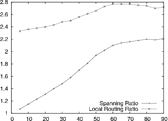
Figure 9 and Table 1 show the results we obtained for the spanning ratio. Figure 10 and Table 2 show the results we obtained for the local routing ratio. For the spanning ratio, the 95% confidence interval for these values is . For the local routing ratio, the 95% confidence interval is .
One interesting conclusion we can draw from these results is that for the spanning ratio, has a more decisive influence than . Figure 11 shows the simulation results for the cases where . We see that even though both ratios generally increase when increase, the spanning ratio varies between 1.07 and 2.21 (107% variation), while the local routing ratio only varies between 2.33 and 2.77 (19% variation). For the local routing ratio, it is the other way around. It is which has a more decisive influence. Figure 12 shows the influence of when . In that case, the local routing ratio varies between 1.72 and 4.55 (165% variation), while the spanning ratio only varies between 1.52 and 1.81 (19% variation).
6 Conclusion
We conclude with the problem that initiated this research. Determine whether or not HSP is a strong -spanner for some constant .
References
- Bose et al. [2006] P. Bose, L. Devroye, W. Evans, and D. Kirkpatrick, On the spanning ratio of Gabriel graphs and -skeletons. SIAM Journal of Disc. Math., 20(2):412–427, 2006.
- Bose et al. [2004] P. Bose, A. Maheshwari, G. Narasimhan, M. Smid, and N. Zeh, Approximating geometric bottleneck shortest paths. Comput. Geom. Theory Appl., 29(3):233–249, 2004.
- Bose and Morin [2004] P. Bose and P. Morin, Online routing in triangulations. SIAM J. Comput., 33(4):937–951, 2004.
- Chavez et al. [2005] E. Chavez, S. Dobrev, E. Kranakis, J. Opatrny, L. Stacho, H. Tejeda, and J. Urrutia, Half-space proximal: A new local test for extracting a bounded dilation spanner. In Springer-Verlag, ed., OPODIS’ 05: Proceedings of the 9th International Conference on Principles of Distributed Systems, 2005.
- Keil and Gutwin [1992] J. M. Keil and C. A. Gutwin, Classes of graphs which approximate the complete euclidean graph. Discrete Comput. Geom., 7(1):13–28, 1992.
- Narasimhan and Smid [2007] G. Narasimhan and M. Smid, Geometric Spanner Networks. Cambridge University Press, New York, NY, USA, 2007.
- Yao [1982] A. C.-C. Yao, On constructing minimum spanning trees in k-dimensional spaces and related problems. SIAM J. Comput., 11(4):721–736, 1982.

| 0.5 | 0.55 | 0.60 | 0.65 | 0.70 | 0.75 | 0.80 | 0.85 | 0.90 | 0.95 | 1 | |
|---|---|---|---|---|---|---|---|---|---|---|---|
| 5 | 1.07 | 1.07 | 1.07 | 1.07 | 1.07 | 1.07 | 1.07 | 1.07 | 1.07 | 1.07 | 1.07 |
| 10 | 1.14 | 1.15 | 1.15 | 1.15 | 1.15 | 1.15 | 1.15 | 1.15 | 1.15 | 1.15 | 1.15 |
| 15 | 1.20 | 1.23 | 1.23 | 1.23 | 1.23 | 1.23 | 1.23 | 1.23 | 1.23 | 1.23 | 1.23 |
| 20 | 1.26 | 1.31 | 1.31 | 1.31 | 1.31 | 1.31 | 1.31 | 1.31 | 1.31 | 1.31 | 1.31 |
| 25 | 1.31 | 1.40 | 1.40 | 1.39 | 1.40 | 1.40 | 1.39 | 1.40 | 1.40 | 1.39 | 1.39 |
| 30 | 1.36 | 1.45 | 1.49 | 1.48 | 1.48 | 1.48 | 1.48 | 1.48 | 1.48 | 1.48 | 1.48 |
| 35 | 1.41 | 1.50 | 1.58 | 1.58 | 1.58 | 1.58 | 1.59 | 1.58 | 1.58 | 1.58 | 1.59 |
| 40 | 1.46 | 1.57 | 1.64 | 1.69 | 1.69 | 1.70 | 1.71 | 1.70 | 1.70 | 1.68 | 1.69 |
| 45 | 1.52 | 1.60 | 1.71 | 1.78 | 1.81 | 1.81 | 1.81 | 1.81 | 1.80 | 1.81 | 1.81 |
| 50 | 1.56 | 1.65 | 1.75 | 1.82 | 1.90 | 1.94 | 1.95 | 1.95 | 1.95 | 1.94 | 1.95 |
| 55 | 1.59 | 1.69 | 1.80 | 1.89 | 1.96 | 2.02 | 2.06 | 2.11 | 2.10 | 2.09 | 2.09 |
| 60 | 1.61 | 1.72 | 1.83 | 1.94 | 2.05 | 2.10 | 2.15 | 2.21 | 2.22 | 2.25 | 2.25 |
| 65 | 1.65 | 1.75 | 1.86 | 1.95 | 2.05 | 2.14 | 2.20 | 2.28 | 2.31 | 2.34 | 2.39 |
| 70 | 1.66 | 1.77 | 1.88 | 1.99 | 2.09 | 2.16 | 2.24 | 2.29 | 2.36 | 2.42 | 2.46 |
| 75 | 1.66 | 1.77 | 1.88 | 2.00 | 2.09 | 2.18 | 2.26 | 2.34 | 2.39 | 2.45 | 2.50 |
| 80 | 1.67 | 1.79 | 1.88 | 1.99 | 2.10 | 2.20 | 2.27 | 2.36 | 2.42 | 2.47 | 2.52 |
| 85 | 1.66 | 1.78 | 1.89 | 2.00 | 2.10 | 2.19 | 2.27 | 2.35 | 2.42 | 2.47 | 2.51 |
| 90 | 1.67 | 1.78 | 1.89 | 2.00 | 2.09 | 2.21 | 2.26 | 2.33 | 2.41 | 2.46 | 2.54 |

| 0.5 | 0.55 | 0.60 | 0.65 | 0.70 | 0.75 | 0.80 | 0.85 | 0.90 | 0.95 | 1 | |
|---|---|---|---|---|---|---|---|---|---|---|---|
| 5 | 1.08 | 1.22 | 1.41 | 1.65 | 1.97 | 2.33 | 2.72 | 3.17 | 3.68 | 4.22 | 4.92 |
| 10 | 1.15 | 1.27 | 1.45 | 1.70 | 2.01 | 2.36 | 2.76 | 3.21 | 3.70 | 4.23 | 4.90 |
| 15 | 1.23 | 1.35 | 1.51 | 1.75 | 2.04 | 2.38 | 2.76 | 3.21 | 3.72 | 4.27 | 4.90 |
| 20 | 1.31 | 1.43 | 1.59 | 1.81 | 2.07 | 2.40 | 2.77 | 3.21 | 3.67 | 4.22 | 4.84 |
| 25 | 1.39 | 1.51 | 1.66 | 1.87 | 2.12 | 2.43 | 2.79 | 3.17 | 3.65 | 4.13 | 4.73 |
| 30 | 1.48 | 1.59 | 1.74 | 1.92 | 2.17 | 2.48 | 2.80 | 3.21 | 3.63 | 4.19 | 4.66 |
| 35 | 1.56 | 1.68 | 1.82 | 2.00 | 2.23 | 2.50 | 2.83 | 3.23 | 3.60 | 4.14 | 4.60 |
| 40 | 1.64 | 1.76 | 1.90 | 2.08 | 2.29 | 2.56 | 2.87 | 3.23 | 3.65 | 4.07 | 4.58 |
| 45 | 1.72 | 1.84 | 1.99 | 2.15 | 2.37 | 2.61 | 2.92 | 3.24 | 3.69 | 4.06 | 4.55 |
| 50 | 1.81 | 1.92 | 2.07 | 2.25 | 2.45 | 2.66 | 2.95 | 3.30 | 3.67 | 4.10 | 4.58 |
| 55 | 1.90 | 2.01 | 2.17 | 2.33 | 2.51 | 2.73 | 2.98 | 3.31 | 3.66 | 4.08 | 4.50 |
| 60 | 1.99 | 2.10 | 2.23 | 2.37 | 2.55 | 2.77 | 3.00 | 3.31 | 3.65 | 4.03 | 4.45 |
| 65 | 2.08 | 2.18 | 2.29 | 2.44 | 2.58 | 2.77 | 3.01 | 3.28 | 3.61 | 3.96 | 4.40 |
| 70 | 2.15 | 2.23 | 2.33 | 2.45 | 2.60 | 2.77 | 3.00 | 3.26 | 3.59 | 3.92 | 4.31 |
| 75 | 2.18 | 2.26 | 2.34 | 2.46 | 2.60 | 2.75 | 2.94 | 3.19 | 3.46 | 3.80 | 4.24 |
| 80 | 2.20 | 2.28 | 2.36 | 2.44 | 2.58 | 2.74 | 2.91 | 3.13 | 3.37 | 3.67 | 4.08 |
| 85 | 2.22 | 2.27 | 2.36 | 2.47 | 2.58 | 2.70 | 2.87 | 3.05 | 3.32 | 3.55 | 3.87 |
| 90 | 2.21 | 2.27 | 2.34 | 2.45 | 2.57 | 2.72 | 2.88 | 3.05 | 3.22 | 3.47 | 3.76 |