跳到论文正文
W Papers独立论文阅读器 arXiv:cs/0702099 论文正文 计算阅读时间 · 0%
引用这篇论文根据当前论文元数据生成,正式投稿前建议核对。


License: Assumed arXiv.org perpetual non-exclusive license
arXiv:cs/0702099v2 [cs.IT] 11 Dec 2007

Discrete Memoryless Interference and Broadcast Channels with Confidential Messages:
Secrecy Rate Regions

Ruoheng Liu       Ivana Marić       Predrag Spasojević          Roy D. Yates Thanks: Manuscript received February 16, 2007; revised July 30, 2007 and October 15, 2007. This work was supported by NSF Grant ANI 0338805. The material in this paper was presented in part at the 44th Allerton Conference on Communication, Control, and Computing, Urbana, IL, USA, September, 2006 and Information Theory and Application Workshop (ITA), San Diego, CA, USA Jan-Feb, 2007. Thanks: R. Liu is with Department of Electrical Engineering, Princeton University, Princeton, NJ 08544 USA (email:˜rliu@princeton.edu). Thanks: P. Spasojević and R. D. Yates are with WINLAB, Electrical and Computer Engineering, Rutgers University, North Brunswick, NJ 08902 USA (email:˜ {spasojev,ryates}@winlab.rutgers.edu). Thanks: I. Marić is with WSL, Department of Electrical Engineering, Stanford University, Stanford, CA 94305 (email:˜ivanam@wsl.stanford.edu).
Abstract

We study information-theoretic security for discrete memoryless interference and broadcast channels with independent confidential messages sent to two receivers. Confidential messages are transmitted to their respective receivers with information-theoretic secrecy. That is, each receiver is kept in total ignorance with respect to the message intended for the other receiver. The secrecy level is measured by the equivocation rate at the eavesdropping receiver. In this paper, we present inner and outer bounds on secrecy capacity regions for these two communication systems. The derived outer bounds have an identical mutual information expression that applies to both channel models. The difference is in the input distributions over which the expression is optimized. The inner bound rate regions are achieved by random binning techniques. For the broadcast channel, a double-binning coding scheme allows for both joint encoding and preserving of confidentiality. Furthermore, we show that, for a special case of the interference channel, referred to as the switch channel, the two bound bounds meet. Finally, we describe several transmission schemes for Gaussian interference channels and derive their achievable rate regions while ensuring mutual information-theoretic secrecy. An encoding scheme in which transmitters dedicate some of their power to create artificial noise is proposed and shown to outperform both time-sharing and simple multiplexed transmission of the confidential messages.

I Introduction

The broadcast nature of a wireless medium allows for the transmitted signal to be received by all users within the communication range. Hence, wireless communication sessions are very susceptible to eavesdropping. The information-theoretic single user secure communication problem was first characterized using the wiretap channel model proposed by Wyner [1]. In this model, a single source-destination communication link is eavesdropped by a wiretapper via a degraded channel. The secrecy level is measured by the equivocation rate at the wiretapper. Wyner showed that secure communication is possible without sharing a secret key between legitimate users, and determined the tradeoff between the transmission rate and the secrecy level [1]. This result was generalized by Csiszár and Körner who determined the capacity region of the broadcast channel with confidential messages [2] in which a message intended for one of the receivers is confidential.

Following the work of Wyner [1] and Csiszár and Körner [2], the more recent information-theoretic research on secure communication focuses at implementing security on the physical layer. Based on independent efforts, the authors of [3] and [4] described achievable secure rate regions and outer bounds for a two-user discrete memoryless multiple access channel with confidential messages. This model generalizes the multiple access channel (MAC) [5, Sec. 14.3] by allowing each user (or one of the users) to receive noisy channel outputs and, hence, to eavesdrop the confidential information sent by the other user. In addition, the Gaussian MAC wiretap channel has been analyzed in [6, 7, 8, 9, 10]. The relay channel with confidential messages where the relay node acts as both a helper and a wiretapper has been considered in [11]. The relay-eavesdropper channel has been proposed in [12]. More recently, the cognitive interference channel with confidential messages has been addressed in [13]. The effects of fading on secure wireless communication have been studied in [14, 15, 16, 17, 18].

In this paper, we study two distinct but related in multi-terminal secure communication problems following the information-theoretic approach. We focus on discrete memoryless interference and broadcast channels with independent confidential messages sent to two receivers. Confidential messages are transmitted to their respective receivers while ensuring mutual information-theoretic secrecy. That is, each receiver is kept in total ignorance with respect to the message intended for the other receiver. We first derive outer bounds on capacity regions for these two communication systems. These bounds have an identical mutual information expression. The expression is optimized over different input distributions, i.e., for the interference channel, the two senders offer independent inputs to the channel and, for the broadcast channel, the sender jointly encodes both messages. We also derive achievable rate regions for the two channel models. Here, we only consider sending confidential messages and, hence, no common message in the sense of Marton [19] is conveyed to the receivers in the case of the broadcast channel. The inner bounds are achieved using random binning techniques. For the broadcast channel, a double-binning coding scheme which allows for both joint precoding as in the classical broadcast channel [19], and preserving of confidentiality. Similarly, ensuring of confidential messages precludes partial decoding of the message intended for the other receiver in the case of the interference channel. Hence, rate-splitting encoding used by Carleial [20] and Han and Kobayashi [21] employed with the classical interference channel is precluded. Instead, the encoders will use only stochastic encoders. We show that for the special case of the interference channel, referred to as the switch channel, derived bounds meet. Finally, we describe several transmission schemes for general Gaussian interference channels and derive their achievable rate regions while still ensuring information-theoretic secrecy. An encoding scheme in which transmitters dedicate some of their power to create artificial noise is proposed and shown to outperform both time-sharing and simple multiplexed transmission of the confidential messages.

The remainder of this paper is organized as follows. The notation and the channel model are given in Sec. II. We state the main results in Sec. III. Outer bounds are derived in Sec. IV. Inner bounds associated with the achievable coding scheme for the interference and broadcast channels with confidential messages are established in Sec. V. Finally, the results are summarized in Sec. VI.

II Definitions and Notations

II-A Notations

Throughout the paper, a random variable is denoted with an upper case letter (e.g., XX), its realization is denoted with the corresponding lower case letter (e.g., xx), the finite alphabet of the random variable is denoted with the corresponding calligraphic letter (e.g., 𝒳{\mathcal{X}}), and its probability distribution is denoted with PX​(x)P_{X}(x). For example, the random variable XX with probability distribution P​(x)=PX​(x)P(x)=P_{X}(x) takes on values in the finite alphabet 𝒳{\mathcal{X}}. A boldface symbol denotes a sequence with the following conventions

𝐗\displaystyle\mathbf{X} =[X1,…,Xn],𝐗i=[X1,…,Xi],\displaystyle=[X_{1},\dots,X_{n}],\quad\mathbf{X}^{i}=[X_{1},\dots,X_{i}],
and 𝐗~i\displaystyle{\tilde{\mathbf{X}}}^{i} =[Xi,…,Xn].\displaystyle=[X_{i},\dots,X_{n}].

Finally, we use Aϵ(n)​(PX)A^{(n)}_{\epsilon}(P_{X}) to denote the set of (weakly) jointly typical sequences 𝐱\mathbf{x} with respect to P⁡(x)P(x) (see [5] for more details).

II-B The Interference Channel with Confidential Messages

Consider a discrete memoryless interference channel with finite input alphabets 𝒳1{\mathcal{X}}_{1}, 𝒳2{\mathcal{X}}_{2}, finite output alphabets 𝒴1{\mathcal{Y}}_{1}, 𝒴2{\mathcal{Y}}_{2}, and the channel transition probability distribution P(y1,y2|x1,x2)P(y_{1},y_{2}|x_{1},x_{2}). Two transmitters wish to send independent, confidential messages to their respective receivers. We refer to such a channel as the interference channel with confidential messages (IC-CM). This communication model is shown in Fig. 1. Symbols (x1,x2)∈(𝒳1×𝒳2)(x_{1},x_{2})\in({\mathcal{X}}_{1}\times{\mathcal{X}}_{2}) are the channel inputs at transmitters 11 and 22, and (y1,y2)∈(𝒴1×𝒴2)(y_{1},y_{2})\in({\mathcal{Y}}_{1}\times{\mathcal{Y}}_{2}) are the channel outputs at receivers 11 and 22, respectively.

Refer to caption

Fig. 1: Interference Channel with Confidential Messages.

Transmitter tt, t=1,2t=1,2, intends to send an independent message Wt∈{1,…,Mt}W_{t}\in\{1,\dots,M_{t}\} to the desired receiver tt in nn channel uses while ensuring information-theoretic secrecy. The channel is memoryless in the sense that

P(𝐲1,𝐲2|𝐱1,𝐱2)=∏i=1nP(y1,i,y2,i|x1,i,x2,i).\displaystyle P(\mathbf{y}_{1},\mathbf{y}_{2}|\mathbf{x}_{1},\mathbf{x}_{2})=\prod_{i=1}^{n}P(y_{1,i},y_{2,i}|x_{1,i},x_{2,i}).

A stochastic encoder for transmitter tt is described by a matrix of conditional probabilities ft​(𝐱t|wt)f_{t}(\mathbf{x}_{t}|w_{t}), where 𝐱t∈𝒳tn\mathbf{x}_{t}\in{\mathcal{X}}_{t}^{n}, wt∈𝒲tw_{t}\in{\mathcal{W}}_{t}, and

∑𝐱t∈𝒳tnft​(𝐱t|wt)=1.\displaystyle\sum_{\mathbf{x}_{t}\in{\mathcal{X}}_{t}^{n}}f_{t}(\mathbf{x}_{t}|w_{t})=1.

Decoding functions are mappings ψt:𝒴t→𝒲t\psi_{t}\,:\,{\mathcal{Y}}_{t}\rightarrow{\mathcal{W}}_{t}. Secrecy levels at receivers 11 and 22 are measured with respect to the equivocation rates

1n​H​(W2|𝐘1)and1n​H​(W1|𝐘2).\frac{1}{n}H(W_{2}|\mathbf{Y}_{1})\quad\text{and}\quad\frac{1}{n}H(W_{1}|\mathbf{Y}_{2}). (1)

An (M1,M2,n,Pe(n))(M_{1},M_{2},n,P^{(n)}_{e}) code for the interference channel consists of two encoding functions f1f_{1}, f2f_{2}, two decoding functions ψ1\psi_{1}, ψ2\psi_{2}, and the corresponding maximum average error probability

Pe(n)≜max⁡{Pe,1(n),Pe,2(n)}\displaystyle P^{(n)}_{e}\triangleq\max\{P_{e,1}^{(n)},\,P_{e,2}^{(n)}\} (2)

where, for t=1,2t=1,2,

Pe,t(n)\displaystyle P_{e,t}^{(n)} =∑w1,w21M1​M2​P​[ψt​(𝐘t)≠wt|(w1,w2)​sent].\displaystyle=\sum_{w_{1},w_{2}}\frac{1}{M_{1}M_{2}}P\bigl[\psi_{t}(\mathbf{Y}_{t})\neq w_{t}|(w_{1},w_{2})~\text{sent}\bigr].

A rate pair (R1,R2)(R_{1},\,R_{2}) is said to be achievable for the interference channel with confidential messages if, for any ϵ0>0\epsilon_{0}>0, there exists a (M1,M2,n,Pe(n))(M_{1},M_{2},n,P^{(n)}_{e}) code such that

Mt≥2n​Rtfor​t=1,2\displaystyle M_{t}\geq 2^{nR_{t}}\quad\text{for}~t=1,2 (3)

and the reliability requirement

Pe(n)\displaystyle P^{(n)}_{e} ≤ϵ0\displaystyle\leq\epsilon_{0} (4)

and the security constraints

n​R1−H⁡(W1|𝐘2)\displaystyle nR_{1}-H(W_{1}|\mathbf{Y}_{2}) ≤n​ϵ0\displaystyle\leq n\epsilon_{0} (5a)
n​R2−H⁡(W2|𝐘1)\displaystyle nR_{2}-H(W_{2}|\mathbf{Y}_{1}) ≤n​ϵ0\displaystyle\leq n\epsilon_{0} (5b)

are satisfied. This definition corresponds to the so-called weak secrecy-key rate [22]. A stronger measurement of the secrecy level has been defined by Maurer and Wolf in terms of the absolute equivocation [22], where the authors have shown that the former definition could be replaced by the latter without any rate penalty for the wiretap channel.

The capacity region of the IC-CM is the closure of the set of all achievable rate pairs (R1,R2)(R_{1},R_{2}), denoted by ℂIC{\mathbb{C}}_{\rm IC}.

II-C The Broadcast Channel

Refer to caption

Fig. 2: Broadcast Channel with Confidential Messages.

We also consider the broadcast channel with confidential messages (BC-CM) in which secret messages from a single transmitter are to be communicated to two receivers, as shown in Fig. 2. A discrete memoryless BC-CM is described using finite sets 𝒳{\mathcal{X}}, 𝒴1{\mathcal{Y}}_{1}, 𝒴2,{\mathcal{Y}}_{2}, and a conditional probability distribution P⁡(y1,y2|x)P(y_{1},y_{2}|x). Symbols x∈𝒳x\in{\mathcal{X}} are channel inputs and (y1,y2)∈(𝒴1×𝒴2)(y_{1},y_{2})\in({\mathcal{Y}}_{1}\times{\mathcal{Y}}_{2}) are channel outputs at receivers 11 and 22, respectively. The transmitter intends to send an independent message Wt∈{1,…,Mt}≜𝒲tW_{t}\in\{1,\dots,M_{t}\}\triangleq{\mathcal{W}}_{t} to the respective receiver t∈{1, 2}t\in\{1,\,2\} in nn channel uses while ensuring information-theoretic secrecy as given by (5a) and (5b). The channel is memoryless in the sense that

P⁡(𝐲1,𝐲2|𝐱)=∏i=1nP⁡(y1,i,y2,i|xi).\displaystyle P(\mathbf{y}_{1},\mathbf{y}_{2}|\mathbf{x})=\prod_{i=1}^{n}P(y_{1,i},y_{2,i}|x_{i}).

A stochastic encoder is specified by a matrix of conditional probabilities f⁡(𝐱|w1,w2)f(\mathbf{x}|w_{1},w_{2}), where 𝐱∈𝒳n\mathbf{x}\in{\mathcal{X}}^{n}, wt∈𝒲tw_{t}\in{\mathcal{W}}_{t}, and

∑𝐱∈𝒳nf⁡(𝐱|w1,w2)=1.\displaystyle\sum_{\mathbf{x}\in{\mathcal{X}}^{n}}f(\mathbf{x}|w_{1},w_{2})=1.

Note that f⁡(𝐱|w1,w2)f(\mathbf{x}|w_{1},w_{2}) is the probability that the pair of messages (w1,w2)(w_{1},w_{2}) are encoded as the channel input 𝐱\mathbf{x}. The decoding function at the receiver tt is a mapping ϕt:𝒴t→𝒲t\phi_{t}\,:\,{\mathcal{Y}}_{t}\rightarrow{\mathcal{W}}_{t}.

The secrecy levels of confidential messages W2W_{2} and W1W_{1} are measured, respectively, at receivers 1 and 2 in terms of the equivocation rates (1). An (M1,M2,n,Pe(n))(M_{1},M_{2},n,P^{(n)}_{e}) code for the broadcast channel consists of the encoding function ff, decoding functions ϕ1\phi_{1}, ϕ2\phi_{2}, and the maximum error probability Pe(n)P^{(n)}_{e} in (2), where, for t=1,2t=1,2,

Pe,t(n)\displaystyle P^{(n)}_{e,t} =∑w1,w21M1​M2​P​[ϕt​(𝐘t)≠wt|(w1,w2)​sent].\displaystyle=\sum_{w_{1},w_{2}}\frac{1}{M_{1}M_{2}}P\bigl[\phi_{t}(\mathbf{Y}_{t})\neq w_{t}|(w_{1},w_{2})~\text{sent}\bigr]. (6)

A rate pair (R1,R2)(R_{1},\,R_{2}) is said to be achievable for the broadcast channel with confidential messages if, for any ϵ0>0\epsilon_{0}>0, there exists a (M1,M2,n,Pe(n))(M_{1},M_{2},n,P^{(n)}_{e}) code which satisfies (3)–(5).

The capacity region of the BC-CM is the closure of the set of all achievable rate pairs (R1,R2)(R_{1},R_{2}), denoted by ℂBC{\mathbb{C}}_{\rm BC}.

III Main Results

In this section, we state our main results. We first describe the outer and inner bounds on the capacity regions of both interference and broadcast channels with confidential messages. We then show that the derived bounds meet for a special case of the interference channel, called the switch channel. Finally, we propose several transmission schemes for Gaussian interference channels and derive their achievable rate regions under information-theoretic secrecy.

III-A Interference Channel with Confidential Messages

Let UU, V1V_{1}, and V2V_{2} be auxiliary random variables. We consider the following two classes of joint distributions for the interference channel. Let πIC−O\pi_{\rm IC-O} be the class of distributions P⁡(u,v1,v2,x1,x2,y1,y2)P(u,v_{1},v_{2},x_{1},x_{2},y_{1},y_{2}) that factor as

P(u)P(v1,v2|u)P(x1|v1)P(x2|v2)P(y1,y2|x1,x2),P(u)P(v_{1},v_{2}|u)P(x_{1}|v_{1})P(x_{2}|v_{2})P(y_{1},y_{2}|x_{1},x_{2}), (7)

and πIC−I\pi_{\rm IC-I} be the class of distributions that factor as

P(u)P(v1|u)P(v2|u)P(x1|v1)P(x2|v2)P(y1,y2|x1,x2).P(u)P(v_{1}|u)P(v_{2}|u)P(x_{1}|v_{1})P(x_{2}|v_{2})P(y_{1},y_{2}|x_{1},x_{2}). (8)
Theorem 1

[outer bound for IC-CM] Let ℝO​(πIC−O){{\mathbb{R}}}_{\rm O}(\pi_{\rm IC-O}) denote the union of all (R1,R2)(R_{1},R_{2}) satisfying

0≤R1\displaystyle 0\leq R_{1} ≤min⁡[I⁡(V1;Y1|U)−I⁡(V1;Y2|U),I(V1;Y1|V2,U)−I(V1;Y2|V2,U)]\displaystyle\leq\min\left[\begin{array}[]{l}I(V_{1};Y_{1}|U)-I(V_{1};Y_{2}|U),\\ I(V_{1};Y_{1}|V_{2},U)-I(V_{1};Y_{2}|V_{2},U)\end{array}\right]
0≤R2\displaystyle 0\leq R_{2} ≤min⁡[I⁡(V2;Y2|U)−I⁡(V2;Y1|U),I(V2;Y2|V1,U)−I(V2;Y1|V1,U)]\displaystyle\leq\min\left[\begin{array}[]{l}I(V_{2};Y_{2}|U)-I(V_{2};Y_{1}|U),\\ I(V_{2};Y_{2}|V_{1},U)-I(V_{2};Y_{1}|V_{1},U)\end{array}\right]

over all distributions P⁡(u,v1,v2,x1,x2,y1,y2)P(u,v_{1},v_{2},x_{1},x_{2},y_{1},y_{2}) in πIC−O\pi_{\rm IC-O}. For the interference channel (𝒳1×𝒳2,P(y1,y2|x1,x2),𝒴1×𝒴2)({\mathcal{X}}_{1}\times{\mathcal{X}}_{2},P(y_{1},y_{2}|x_{1},x_{2}),{\mathcal{Y}}_{1}\times{\mathcal{Y}}_{2}) with confidential messages, the capacity region

ℂIC⊆ℝO​(πIC−O).{\mathbb{C}}_{\rm IC}\subseteq{\mathbb{R}}_{\rm O}(\pi_{\rm IC-O}).
Proof:

We provide the proof of Theorem 1 in Sec. IV. ∎

Theorem 2

[inner bound for IC-CM] Let ℝIC​(πIC−I){{\mathbb{R}}}_{\rm IC}(\pi_{\rm IC-I}) denote the union of all (R1,R2)(R_{1},R_{2}) satisfying

0\displaystyle 0 ≤R1≤I(V1;Y1|U)−I(V1;Y2|V2,U)\displaystyle\leq R_{1}\leq I(V_{1};Y_{1}|U)-I(V_{1};Y_{2}|V_{2},U) (10a)
0\displaystyle 0 ≤R2≤I(V2;Y2|U)−I(V2;Y1|V1,U)\displaystyle\leq R_{2}\leq I(V_{2};Y_{2}|U)-I(V_{2};Y_{1}|V_{1},U) (10b)

over all distributions P⁡(u,v1,v2,x1,x2,y1,y2)P(u,v_{1},v_{2},x_{1},x_{2},y_{1},y_{2}) in πIC−I\pi_{\rm IC-I}. Any rate pair

(R1,R2)∈ℝIC​(πIC−I)(R_{1},R_{2})\in{\mathbb{R}}_{\rm IC}(\pi_{\rm IC-I})

is achievable for the interference channel with confidential messages.

Proof:

We provide the proof in Sec. V-A. ∎

To derive the achievable rate region for the IC-CM, we employ an auxiliary random variable UU in the sense of Han-Kobayashi [21]. For a given UU, we consider two independent stochastic encoders, that is, the pre-coding auxiliary random variables V1V_{1} and V2V_{2} will be independent for a given UU, as given by (8). To ensure information-theoretic secrecy, the achievable rate R1R_{1} includes a penalty term I(V1;Y2|V2,U)I(V_{1};Y_{2}|V_{2},U), which is a conditional mutual information of the receiver 2’s eavesdropper channel while assuming the receiver 2 can first decode its own information.

III-B Broadcast Channel with Confidential Messages

For the broadcast channel, we focus on the class of distributions P⁡(u,v1,v2,x,y1,y2)P(u,v_{1},v_{2},x,y_{1},y_{2}) that factor as

P⁡(u)​P​(v1,v2|u)​P​(x|v1,v2)​P​(y1,y2|x).P(u)P(v_{1},v_{2}|u)P(x|v_{1},v_{2})P(y_{1},y_{2}|x). (11)

We refer to this class as πBC\pi_{\rm BC}.

Theorem 3

[outer bound for BC-CM] Let ℝO​(πBC){{\mathbb{R}}}_{\rm O}(\pi_{\rm BC}) denote the union of all (R1,R2)(R_{1},R_{2}) satisfying

R1\displaystyle R_{1} ≥0,R2≥0\displaystyle\geq 0,~R_{2}\geq 0
R1\displaystyle R_{1} ≤min⁡[I⁡(V1;Y1|U)−I⁡(V1;Y2|U),I(V1;Y1|V2,U)−I(V1;Y2|V2,U)]\displaystyle\leq\min\left[\begin{array}[]{l}I(V_{1};Y_{1}|U)-I(V_{1};Y_{2}|U),\\ I(V_{1};Y_{1}|V_{2},U)-I(V_{1};Y_{2}|V_{2},U)\end{array}\right]
R2\displaystyle R_{2} ≤min⁡[I⁡(V2;Y2|U)−I⁡(V2;Y1|U),I(V2;Y2|V1,U)−I(V2;Y1|V1,U)]\displaystyle\leq\min\left[\begin{array}[]{l}I(V_{2};Y_{2}|U)-I(V_{2};Y_{1}|U),\\ I(V_{2};Y_{2}|V_{1},U)-I(V_{2};Y_{1}|V_{1},U)\end{array}\right]

over all distributions P⁡(u,v1,v2,x,y1,y2)P(u,v_{1},v_{2},x,y_{1},y_{2}) in πBC\pi_{\rm BC} and auxiliary random variables UU, V1V_{1}, and V2V_{2} satisfying

U\displaystyle U →V1→XandU→V2→X.\displaystyle\rightarrow V_{1}\rightarrow X\quad\text{and}\quad U\rightarrow V_{2}\rightarrow X. (13)

For the broadcast channel (𝒳,P⁡(y1,y2|x),𝒴1×𝒴2)({\mathcal{X}},P(y_{1},y_{2}|x),{\mathcal{Y}}_{1}\times{\mathcal{Y}}_{2}) with confidential messages, the capacity region

ℂBC⊆ℝO​(πBC).{\mathbb{C}}_{\rm BC}\subseteq{\mathbb{R}}_{\rm O}(\pi_{\rm BC}).
Proof:

We provide the proof of Theorem 3 in Sec. IV. ∎

Remark 1

Outer bounds for the BC-CM and the IC-CM have a same mutual information expression ℝO​(⋅){\mathbb{R}}_{\rm O}(\cdot), but, they are optimized over different input distributions πBC\pi_{\rm BC} and πIC−O\pi_{\rm IC-O}, respectively.

Theorem 4

[inner bound for BC-CM] Let ℝBC​(πBC){{\mathbb{R}}}_{\rm BC}(\pi_{\rm BC}) denote the union of all (R1,R2)(R_{1},R_{2}) satisfying

R1\displaystyle R_{1} ≥0,R2≥0\displaystyle\geq 0,~R_{2}\geq 0
R1\displaystyle R_{1} ≤I(V1;Y1|U)−I(V1;V2|U)−I(V1;Y2|V2,U)\displaystyle\leq I(V_{1};Y_{1}|U)-I(V_{1};V_{2}|U)-I(V_{1};Y_{2}|V_{2},U) (14a)
R2\displaystyle R_{2} ≤I(V2;Y2|U)−I(V1;V2|U)−I(V2;Y1|V1,U)\displaystyle\leq I(V_{2};Y_{2}|U)-I(V_{1};V_{2}|U)-I(V_{2};Y_{1}|V_{1},U) (14b)

over all distributions P⁡(u,v1,v2,x,y1,y2)P(u,v_{1},v_{2},x,y_{1},y_{2}) in πBC\pi_{\rm BC}. Any rate pair

(R1,R2)∈ℝBC​(πBC)(R_{1},R_{2})\in{\mathbb{R}}_{\rm BC}(\pi_{\rm BC})

is achievable for the broadcast channel with confidential messages.

Proof:

We provide the proof in Sec. V-B. ∎

We note that, for a broadcast channel, we can employ joint encoding at the transmitter. Hence, the achievable coding scheme for the BC-CM is based on the double-binning scheme which combines the Gel’fand-Pinsker binning [23] and the random binning. To preserve confidentiality, the achievability bounds on R1R_{1} and R2R_{2} each include the penalty term I⁡(V1;V2|U)I(V_{1};V_{2}|U). Without the confidentiality constraint, Marton’s inner bound [19] on the broadcast channel illustrates only that the sum rate has the penalty term I⁡(V1;V2|U)I(V_{1};V_{2}|U). To ensure information-theoretic secrecy, the proposed coding scheme pays “double” when jointly encoding at the transmitter.

Example 1

[less noisy broadcast channel] Consider a special class of broadcast channels in which the channel X→Y1X\rightarrow Y_{1} is less noisy than the channel X→Y2X\rightarrow Y_{2}, i.e.,

I⁡(V,Y1)≥I⁡(V,Y2)\displaystyle I(V;Y_{1})\geq I(V;Y_{2}) (15)

for every V→X→(Y1,Y2)V\rightarrow X\rightarrow(Y_{1},Y_{2}) [2]. We first consider the outer bound of the less noisy BC-CM. Based on the Markov chains in (13) and the definition (15), we have

I⁡(V1;Y1|U=u)\displaystyle I(V_{1};Y_{1}|U=u) ≥I⁡(V1;Y2|U=u)\displaystyle\geq I(V_{1};Y_{2}|U=u)
I⁡(V2;Y1|U=u)\displaystyle I(V_{2};Y_{1}|U=u) ≥I⁡(V2;Y2|U=u),\displaystyle\geq I(V_{2};Y_{2}|U=u),

which implies that

I⁡(V1;Y1|U)\displaystyle I(V_{1};Y_{1}|U) ≥I⁡(V1;Y2|U)\displaystyle\geq I(V_{1};Y_{2}|U)
I⁡(V2;Y1|U)\displaystyle I(V_{2};Y_{1}|U) ≥I⁡(V2;Y2|U).\displaystyle\geq I(V_{2};Y_{2}|U).

Hence the outer bound can be rewritten as the union of all (R1,R2)(R_{1},R_{2}) satisfying

R1\displaystyle R_{1} ≤maxP⁡(X)⁡[I⁡(X,Y1)−I⁡(X,Y2)]\displaystyle\leq\max_{P(X)}[I(X;Y_{1})-I(X;Y_{2})] (16a)
R2\displaystyle R_{2} =0\displaystyle=0 (16b)

where (16a) follows from [2, Theorem 3]. Next, by applying Theorem 4 and setting V2=U=constV_{2}=U=\text{const}, we obtain the identical rate region as (16). This result implies that only the “better” user can get the non-zero secrecy rate for the less noisy BC-CM. Note that, the single-antenna Gaussian broadcast channel is a special case of the less noisy broadcast channel.

In the following, we consider a sufficient condition under which both R1R_{1} and R2R_{2} can be strictly positive for the BC-CM.

Corollary 1

For a broadcast channel, if there exist a distribution P⁡(u,v1,v2,x,y1,y2)∈πBCP(u,v_{1},v_{2},x,y_{1},y_{2})\in\pi_{\rm BC} for which

I⁡(V1;Y1|U)\displaystyle I(V_{1};Y_{1}|U) >I⁡(V1;Y2,V2|U)\displaystyle>I(V_{1};Y_{2},V_{2}|U) (17a)
and I⁡(V2;Y2|U)\displaystyle I(V_{2};Y_{2}|U) >I⁡(V2;Y1,V1|U),\displaystyle>I(V_{2};Y_{1},V_{1}|U), (17b)

then both receivers can achieve strictly positive rates while ensuring information-theoretic secrecy.

Proof:

The result is obtained by applying Theorem 4 and by setting R1>0R_{1}>0 and R2>0R_{2}>0. ∎More recently, motivated by this work, the multiple-antenna Gaussian broadcast channel with confidential messages was studied in [24]. It was shown that with multiple antennas at transmitters, strictly positive rates to both receivers can be achieved while ensuring information-theoretic secrecy.

III-C Switch Channel

In this subsection, we obtain the secrecy capacity region for a special case of the interference channel referred to as the switch channel (SC). As shown in Fig. 3, receivers in the SC cannot listen to both transmissions (from encoders 11 and 22) at the same time. For example, each encoder may transmit at a different frequency, while each receiver may listen only to one frequency during each symbol time ii. We assume that each receiver t∈{1,2}t\in\{1,2\} has a random switch st∈{1,2}s_{t}\in\{1,2\}, which chooses between tt and t¯\bar{t} independently at each symbol time ii with probabilities

P⁡(St,i=t)\displaystyle P(S_{t,i}=t) =τt\displaystyle=\tau_{t}
P⁡(St,i=t¯)\displaystyle P(S_{t,i}=\bar{t}) =1−τt,i=1,…,n\displaystyle=1-\tau_{t},\quad i=1,\dots,n

where t¯\bar{t} is the complement of tt. Therefore, receiver tt listens to its own information xt,ix_{t,i} from encoder tt whenever St,i=tS_{t,i}=t, while it eavesdrops the signal xt¯,ix_{\bar{t},i} when St,i=t¯S_{t,i}=\bar{t}. By assuming that the switch state information is available at the receiver, we have that

P⁡(yt,i|x1,i,x2,i,st,i)\displaystyle P(y_{t,i}|x_{1,i},x_{2,i},s_{t,i}) =P⁡(yt,i|x1,i)​𝟏​(st,i=1)\displaystyle=P(y_{t,i}|x_{1,i}){\bf 1}(s_{t,i}=1)
+P⁡(yt,i|x2,i)​𝟏​(st,i=2)\displaystyle\qquad+P(y_{t,i}|x_{2,i}){\bf 1}(s_{t,i}=2)
=P⁡(yt,i|xst,i,i)\displaystyle=P(y_{t,i}|x_{s_{t,i},i}) (18)

where 𝟏​(⋅){\bf 1}(\cdot) is the indicator function.

Refer to caption

Fig. 3: Switch channel model

The switch state information {St,i}i=1n\{S_{t,i}\}^{n}_{i=1} is an i.i.d. process known at receiver tt. Hence, we can consider st,is_{t,i} as a part of the channel output, i.e., we set

yt,i≜{zt,i,st,i}\displaystyle y_{t,i}\triangleq\{z_{t,i},\,s_{t,i}\} (19)

where zt,iz_{t,i} represents the received signal value at receiver tt. Under this setting, we have the following theorem on the secrecy capacity region ℂSC{\mathbb{C}}_{\rm SC} of SC-CM.

Theorem 5

For the switch channel with confidential messages, the capacity region ℂSC{\mathbb{C}}_{\rm SC} is the union of all (R1,R2)(R_{1},R_{2}) satisfying

0\displaystyle 0 ≤R1≤I(V1;Y1|U)−I(V1;Y2|V2,U)\displaystyle\leq R_{1}\leq I(V_{1};Y_{1}|U)-I(V_{1};Y_{2}|V_{2},U) (20a)
0\displaystyle 0 ≤R2≤I(V2;Y2|U)−I(V2;Y1|V1,U)\displaystyle\leq R_{2}\leq I(V_{2};Y_{2}|U)-I(V_{2};Y_{1}|V_{1},U) (20b)

over all distributions P⁡(u,v1,v2,x1,x2,y1,y2)P(u,v_{1},v_{2},x_{1},x_{2},y_{1},y_{2}) in πIC−I\pi_{\rm IC-I}.

Proof:

We provide the proof in the Appendix. ∎

Remark 2

In SC-CM, receiver tt listens to the desired information during time fraction τt\tau_{t}, and intercepts the other message during the time fraction (1−τt)(1-\tau_{t}). When τ1=τ2=1\tau_{1}=\tau_{2}=1, both receivers only listen to their own messages and thus SC-CM reduces to two independent parallel channels without the secrecy constraints. When τ1=1\tau_{1}=1 and τ2=0\tau_{2}=0, receiver 22 acts as an eavesdropper only and both Y1Y_{1} and Y2Y_{2} are independent with respect to the message W2W_{2}. Hence, in this case, SC-CM reduces to the wiretap channel [1].

Example 2

[noiseless memoryless switch channel] We assume that the channel is discrete memoryless and that the input-output relationship at each time instant satisfies

Yt,i={X1,i,St,i=1X2,i,St,i=2fori=1,…,n\displaystyle Y_{t,i}=\left\{\begin{array}[]{ll}X_{1,i},&S_{t,i}=1\\ X_{2,i},&S_{t,i}=2\end{array}\right.\qquad\text{for}\quad i=1,\dots,n

where P⁡(St,i=t)=τtP(S_{t,i}=t)=\tau_{t} and τ1+τ2≥1\tau_{1}+\tau_{2}\geq 1. Theorem 5 implies that the secrecy capacity region of this channel is:

{(R1,R2):R1≤(τ1+τ2−1)​H​(X1)R2≤(τ1+τ2−1)​H​(X2)}.\displaystyle\left\{(R_{1},R_{2}):\begin{array}[]{l}R_{1}\leq(\tau_{1}+\tau_{2}-1)H(X_{1})\\ R_{2}\leq(\tau_{1}+\tau_{2}-1)H(X_{2})\end{array}\right\}.

We note that here τ1+τ2−1\tau_{1}+\tau_{2}-1 equals τ1−(1−τ2)\tau_{1}-(1-\tau_{2}), the time that user 1 sends without user 2 listening and also equals τ2−(1−τ1)\tau_{2}-(1-\tau_{1}), the time that user 2 sends without user 1 listening.

III-D Gaussian Interference Channel with Confidential Messages

We next consider a Gaussian interference channel (GIC) with confidential messages (GIC-CM) where each node employs a single antenna as shown in Fig. 4. We have proposed this problem originally in [25].

Refer to caption

Fig. 4: Gaussian interference channel with confidential messages

We assume the channel input and output symbols to be from an alphabet of real numbers. Following the standard form GIC [20], the received symbols are

Y1\displaystyle Y_{1} =X1+α1​X2+N1\displaystyle=X_{1}+\alpha_{1}X_{2}+N_{1} (25a)
Y2\displaystyle Y_{2} =α2​X1+X2+N2\displaystyle=\alpha_{2}X_{1}+X_{2}+N_{2} (25b)

where α1\alpha_{1} and α2\alpha_{2} are normalized crossover channel gains, X1X_{1} and X2X_{2} are transmitted symbols from encoders 11 and 22 with the average power constraint

∑i=1nE​[Xt,i2]n≤Pt,fort=1,2,\sum_{i=1}^{n}\frac{\textsf{E}[X^{2}_{t,i}]}{n}\leq P_{t},\quad\text{for}~t=1,2,

and N1N_{1} and N2N_{2} correspond to two independent, zero-mean, unit-variance, Gaussian noise variables. In the following, we focus on the weak interference channel, i.e., 0≤α12<10\leq\alpha_{1}^{2}<1 and 0≤α22<10\leq\alpha_{2}^{2}<1. We describe three transmission schemes and their achievable rate regions under the requirement of information-theoretic secrecy.

III-D1 Time-Sharing

The transmission period is divided into two non-overlapping slots with time fractions ρ1\rho_{1} and ρ2\rho_{2}, where ρ1≥0\rho_{1}\geq 0, ρ2≥0\rho_{2}\geq 0, and ρ1+ρ2=1\rho_{1}+\rho_{2}=1. Transmitter tt sends confidential message WtW_{t} in slot tt with time fraction ρt\rho_{t}, t=1,2t=1,2. We refer to this technique as the time-sharing scheme. We note that, in each slot, the channel reduces to a Gaussian wiretap channel [26]. Let ℝGIC[T]{\mathbb{R}}_{\rm GIC}^{\rm[T]} denote the set of (R1,R2)(R_{1},R_{2}) satisfying

0\displaystyle 0 ≤R1≤ρ12​[log⁡(1+P1ρ1)−log⁡(1+α22​P1ρ1)]\displaystyle\leq R_{1}\leq\frac{\rho_{1}}{2}\left[\log\left(1+\frac{P_{1}}{\rho_{1}}\right)-\log\left(1+\alpha^{2}_{2}\frac{P_{1}}{\rho_{1}}\right)\right]
0\displaystyle 0 ≤R2≤ρ22​[log⁡(1+P2ρ2)−log⁡(1+α12​P2ρ2)]\displaystyle\leq R_{2}\leq\frac{\rho_{2}}{2}\left[\log\left(1+\frac{P_{2}}{\rho_{2}}\right)-\log\left(1+\alpha^{2}_{1}\frac{P_{2}}{\rho_{2}}\right)\right]

over all time fractions (ρ1,ρ2)(\rho_{1},\rho_{2}) pairs. Following [26], we can show that any rate pair

(R1,R2)∈ℝGIC[T](R_{1},R_{2})\in{\mathbb{R}}_{\rm GIC}^{\rm[T]}

is achievable for GIC-CM.

III-D2 Multiplexed Transmission

In the multiplexed transmission scheme, we allow communication links to share the same degrees of freedom. Since we require information-theoretic secrecy for confidential messages, no partial decoding of the other transmitter’s message is allowed at a receiver. Hence, the interference results in an increase of the noise floor. Let

0≤βt≤1,t=1,2.0\leq\beta_{t}\leq 1,\quad t=1,2.

By independently choosing

Vt=Xt∼𝒩[0,βtPt],t=1,2V_{t}=X_{t}\sim{\mathcal{N}}[0,\beta_{t}P_{t}],\quad t=1,2

and letting UU serve as a convex combination operator, Theorem 2 implies that any rate pair

(R1,R2)∈ℝGIC[M](R_{1},R_{2})\in{\mathbb{R}}_{\rm GIC}^{\rm[M]}

is achievable for GIC-CM, where ℝGIC[M]{\mathbb{R}}_{\rm GIC}^{\rm[M]} denotes the convex hull of the set of (R1,R2)(R_{1},R_{2}) satisfying

R1\displaystyle R_{1} ≥0,R2≥0\displaystyle\geq 0,\quad R_{2}\geq 0
R1\displaystyle R_{1} ≤12​log⁡(1+β1​P11+α12​β2​P2)−12​log⁡(1+α22​β1​P1)\displaystyle\leq\frac{1}{2}\log\left(1+\frac{\beta_{1}P_{1}}{1+\alpha^{2}_{1}\beta_{2}P_{2}}\right)-\frac{1}{2}\log(1+\alpha^{2}_{2}\beta_{1}P_{1})
R2\displaystyle R_{2} ≤12​log⁡(1+β2​P21+α22​β1​P1)−12​log⁡(1+α12​β2​P2)\displaystyle\leq\frac{1}{2}\log\left(1+\frac{\beta_{2}P_{2}}{1+\alpha^{2}_{2}\beta_{1}P_{1}}\right)-\frac{1}{2}\log(1+\alpha^{2}_{1}\beta_{2}P_{2})

over all power-control parameters β1\beta_{1} and β2\beta_{2}.

III-D3 Artificial Noise

We next describe a scheme which allows one of the transmitters (e.g., transmitter 22) to generate artificial noise. This strategy involves splitting of the transmission power of transmitter 22 into two parts P2,MP_{2,M} and P2,AP_{2,A}, where

P2,M\displaystyle P_{2,M} =(1−λ)​β2​P2,\displaystyle=(1-\lambda)\beta_{2}P_{2},
P2,A\displaystyle P_{2,A} =λ​β2​P2,and0≤λ≤1,\displaystyle=\lambda\beta_{2}P_{2},\quad\text{and}\quad 0\leq\lambda\leq 1,

so that transmitter 22 encodes the confidential message with power P2,MP_{2,M} and generates artificial noise with power P2,AP_{2,A}. The artificial noise can spoil the received signal of receiver 22 and, hence, protect the confidential message of transmitter 11. In this sense, this scheme allows transmitter cooperation without exchanging confidential messages. Let UU serve as a convex combination operator,

X1\displaystyle X_{1} =V1andX2=V2+A2\displaystyle=V_{1}\quad\text{and}\quad X_{2}=V_{2}+A_{2} (28)

where V1V_{1}, V2V_{2}, and A2A_{2} are independent Gaussian random variables:

V1\displaystyle V_{1} ∼𝒩⁡[0,β1​P1],\displaystyle\sim{\mathcal{N}}[0,\beta_{1}P_{1}],
V2\displaystyle V_{2} ∼𝒩⁡[0,P2,M],\displaystyle\sim{\mathcal{N}}[0,P_{2,M}],
and A2\displaystyle A_{2} ∼𝒩⁡[0,P2,A].\displaystyle\sim{\mathcal{N}}[0,P_{2,A}].

Here A2A_{2} denotes the artificial noise which cannot be predicted and subtracted by either receiver. Since

Y1\displaystyle Y_{1} =X1+α1​X2+N1\displaystyle=X_{1}+\alpha_{1}X_{2}+N_{1}
=V1+α1​(V2+A2)+N1\displaystyle=V_{1}+\alpha_{1}(V_{2}+A_{2})+N_{1}

and

Y2\displaystyle Y_{2} =α2​X1+X2+N1\displaystyle=\alpha_{2}X_{1}+X_{2}+N_{1}
=α2​V1+(V2+A2)+N2,\displaystyle=\alpha_{2}V_{1}+(V_{2}+A_{2})+N_{2},

we have

I⁡(V1,Y1)\displaystyle I(V_{1};Y_{1}) =I⁡(V1,V1+α1​(V2+A2)+N1)\displaystyle=I(V_{1};\,V_{1}+\alpha_{1}(V_{2}+A_{2})+N_{1})
=h⁡(V1+α1​(V2+A2)+N1)\displaystyle=h(V_{1}+\alpha_{1}(V_{2}+A_{2})+N_{1})
−h⁡(α1​(V2+A2)+N1)\displaystyle\quad-h(\alpha_{1}(V_{2}+A_{2})+N_{1})
=12​log⁡(1+β1​P11+α12​β2​P2)\displaystyle=\frac{1}{2}\log\left(1+\frac{\beta_{1}P_{1}}{1+\alpha_{1}^{2}\beta_{2}P_{2}}\right)

and

I⁡(V1;Y2|V2)\displaystyle I(V_{1};Y_{2}|V_{2}) =I⁡(V1;α2​V1+V2+A2+N2|V2)\displaystyle=I(V_{1};\,\alpha_{2}V_{1}+V_{2}+A_{2}+N_{2}|V_{2})
=h⁡(α2​V1+A2+N2)−h⁡(A2+N2)\displaystyle=h(\alpha_{2}V_{1}+A_{2}+N_{2})-h(A_{2}+N_{2})
=12​log⁡(1+α22​β1​P11+λ​β2​P2).\displaystyle=\frac{1}{2}\log\left(1+\frac{\alpha^{2}_{2}\beta_{1}P_{1}}{1+\lambda\beta_{2}P_{2}}\right).

Similarly, we can calculate

I⁡(V2,Y2)\displaystyle I(V_{2};Y_{2}) =12​log⁡[1+(1−λ)​β2​P21+α22​β1​P1+λ​β2​P2]\displaystyle=\frac{1}{2}\log\left[1+\frac{(1-\lambda)\beta_{2}P_{2}}{1+\alpha^{2}_{2}\beta_{1}P_{1}+\lambda\beta_{2}P_{2}}\right]

and

I⁡(V2;Y1|V1)\displaystyle I(V_{2};Y_{1}|V_{1}) =12​log⁡[1+(1−λ)​α12​β2​P21+λ​α12​β2​P2].\displaystyle=\frac{1}{2}\log\left[1+\frac{(1-\lambda)\alpha^{2}_{1}\beta_{2}P_{2}}{1+\lambda\alpha^{2}_{1}\beta_{2}P_{2}}\right].

Applying Theorem 2, we can prove that any rate pair

(R1,R2)∈ℝGIC[A](R_{1},R_{2})\in{\mathbb{R}}_{\rm GIC}^{\rm[A]}

is achievable for GIC-CM, where ℝGIC[A]{\mathbb{R}}_{\rm GIC}^{\rm[A]} denotes the convex hull of the set of (R1,R2)(R_{1},R_{2}) satisfying

0≤R1\displaystyle 0\leq R_{1} ≤12​log⁡(1+β1​P11+α12​β2​P2)\displaystyle\leq\frac{1}{2}\log\left(1+\frac{\beta_{1}P_{1}}{1+\alpha^{2}_{1}\beta_{2}P_{2}}\right)
−12​log⁡(1+α22​β1​P11+λ​β2​P2)\displaystyle\qquad-\frac{1}{2}\log\left(1+\frac{\alpha^{2}_{2}\beta_{1}P_{1}}{1+\lambda\beta_{2}P_{2}}\right) (29a)
0≤R2\displaystyle 0\leq R_{2} ≤12​log⁡[1+(1−λ)​β2​P21+α22​β1​P1+λ​β2​P2]\displaystyle\leq\frac{1}{2}\log\left[1+\frac{(1-\lambda)\beta_{2}P_{2}}{1+\alpha^{2}_{2}\beta_{1}P_{1}+\lambda\beta_{2}P_{2}}\right]
−12​log⁡[1+(1−λ)​α12​β2​P21+λ​α12​β2​P2]\displaystyle\qquad-\frac{1}{2}\log\left[1+\frac{(1-\lambda)\alpha^{2}_{1}\beta_{2}P_{2}}{1+\lambda\alpha^{2}_{1}\beta_{2}P_{2}}\right] (29b)

over all power-control parameter pair (β1,β2)(\beta_{1},\beta_{2}) and the power-splitting parameter λ\lambda. Furthermore, the achievable region can be increased by reversing the roles of transmitters 11 and 22.

Remark 3

We note that secure communication in a Gaussian channel with two senders and two receivers was also considered in [9, 10] for the Gaussian MAC with a wiretapper (GMAC-WT). In this setting, both messages are to be conveyed to one of the receivers and none to the other receiver. Although the two problem formulations differ, the absence of rate splitting in the interference channel results in that the two proposed encoding schemes have a closer relationship than the schemes suggested for the classical MAC and interference channels. In fact, the encoding scheme proposed in [9, 10] for the GMAC-WT, referred to as cooperative jamming, and our encoding scheme which creates artificial noise in (28) are the same.

Refer to caption

a. P1=P2=10P_{1}=P_{2}=10

Refer to caption

a. P1=P2=100P_{1}=P_{2}=100

Fig. 5: Achievability regions for the GIC-CM (α1=α2=0.2\alpha_{1}=\alpha_{2}=0.2).
Example 3

In Fig. 5, we compare the achievable regions:

ℝGIC[T],ℝGIC[M],and​ℝGIC[A]{\mathbb{R}}_{\rm GIC}^{\rm[T]},~{\mathbb{R}}_{\rm GIC}^{\rm[M]},~\text{and}~{\mathbb{R}}_{\rm GIC}^{\rm[A]}

by numerical calculation, for

P1=P2=10​and​α1=α2=0.2P_{1}=P_{2}=10~\text{and}~\alpha_{1}=\alpha_{2}=0.2

in Fig. 5.a and

P1=P2=100​and​α1=α2=0.2P_{1}=P_{2}=100~\text{and}~\alpha_{1}=\alpha_{2}=0.2

in Fig. 5.b. Both numerical results illustrate that the artificial noise strategy allows for communication over larger rates, when compared to the time-sharing and multiplexed transmission schemes.

IV Outer Bound

In this section we prove Theorems 1 and 3. In the following, we derive the upper bound for R1R_{1}. The upper bound for R2R_{2} follows by symmetry.

The basis for the outer bound derivation is the reliable transmission requirement and the security constraint. Based on Fano’s inequality [5], the reliable transmission requirement (4) implies that

H⁡(W1|𝐘1)\displaystyle H(W_{1}|\mathbf{Y}_{1}) ≤ϵ0​log⁡(M1−1)+h⁡(ϵ0)≜n​δ1.\displaystyle\leq\epsilon_{0}\log(M_{1}-1)+h(\epsilon_{0})\triangleq n\delta_{1}. (30a)
H⁡(W2|𝐘2)\displaystyle H(W_{2}|\mathbf{Y}_{2}) ≤ϵ0​log⁡(M2−1)+h⁡(ϵ0)≜n​δ2.\displaystyle\leq\epsilon_{0}\log(M_{2}-1)+h(\epsilon_{0})\triangleq n\delta_{2}. (30b)

where h⁡(x)h(x) is the binary entropy function. On the other hand, the security constraint (5a) implies that

n​R1=H⁡(W1)\displaystyle nR_{1}=H(W_{1}) ≤H⁡(W1|𝐘2)+n​ϵ0.\displaystyle\leq H(W_{1}|\mathbf{Y}_{2})+n\epsilon_{0}. (31)

In fact, the bound (9) on R1R_{1} is based on the following two different upper bounds on the equivocation H⁡(W1|𝐘2)H(W_{1}|\mathbf{Y}_{2}).

IV-A First Bound

The first upper bound is derived by applying the techniques in [2]. By using Fano’s inequality (30a), we obtain the following bound on the equivocation

H⁡(W1|𝐘2)≤H⁡(W1|𝐘2)−H⁡(W1|𝐘1)+n​δ1.\displaystyle H(W_{1}|\mathbf{Y}_{2})\leq H(W_{1}|\mathbf{Y}_{2})-H(W_{1}|\mathbf{Y}_{1})+n\delta_{1}. (32)

Let

Ui=(𝐘1i−1,𝐘~2i+1).\displaystyle U_{i}=(\mathbf{Y}_{1}^{i-1},{\tilde{\mathbf{Y}}}_{2}^{i+1}). (33)

Since (Ui,Y2,i)=(𝐘1i−1,𝐘~2i)=(Ui−1,Y1,i−1)(U_{i},Y_{2,i})=(\mathbf{Y}_{1}^{i-1},{\tilde{\mathbf{Y}}}_{2}^{i})=(U_{i-1},Y_{1,i-1}), we have

H⁡(W1|Ui,Y2,i)−H⁡(W1|Ui−1,Y1,i−1)=0\displaystyle H(W_{1}|U_{i},Y_{2,i})-H(W_{1}|U_{i-1},Y_{1,i-1})=0

and we can rewrite (32) as follows

H⁡(W1|𝐘2)\displaystyle H(W_{1}|\mathbf{Y}_{2}) ≤H⁡(W1|𝐘2)−H⁡(W1|𝐘1)\displaystyle\leq H(W_{1}|\mathbf{Y}_{2})-H(W_{1}|\mathbf{Y}_{1})
+∑i=2n[H(W1|Ui,Y2,i)\displaystyle\quad+\sum_{i=2}^{n}\bigl[H(W_{1}|U_{i},Y_{2,i})
−H(W1|Ui−1,Y1,i−1)]+nδ1.\displaystyle\quad-H(W_{1}|U_{i-1},Y_{1,i-1})\bigr]+n\delta_{1}. (34)

Note that

𝐘1\displaystyle\mathbf{Y}_{1} =(Un,Y1,n)and𝐘2=(U1,Y2,1).\displaystyle=(U_{n},Y_{1,n})\quad\text{and}\quad\mathbf{Y}_{2}=(U_{1},Y_{2,1}).

Hence, the bound (34) can be expressed as follows

H⁡(CLOSE\displaystyle H( OPENW1|𝐘2)\displaystyle W_{1}|\mathbf{Y}_{2})
≤H⁡(W1|U1,Y2,1)−H⁡(W1|Un,Y1,n)\displaystyle\leq H(W_{1}|U_{1},Y_{2,1})-H(W_{1}|U_{n},Y_{1,n})
+∑i=2nH(W1|Ui,Y2,i)−∑i=1n−1H(W1|Ui,Y1,i)+nδ1\displaystyle\quad+\sum_{i=2}^{n}H(W_{1}|U_{i},Y_{2,i})-\sum_{i=1}^{n-1}H(W_{1}|U_{i},Y_{1,i})+n\delta_{1}
=∑i=1n[H⁡(W1|Ui,Y2,i)−H⁡(W1|Ui,Y1,i)]+n​δ1\displaystyle=\sum_{i=1}^{n}[H(W_{1}|U_{i},Y_{2,i})-H(W_{1}|U_{i},Y_{1,i})]+n\delta_{1}
=∑i=1n[I⁡(W1;Y1,i|Ui)−I⁡(W1;Y2,i|Ui)]+n​δ1.\displaystyle=\sum_{i=1}^{n}[I(W_{1};Y_{1,i}|U_{i})-I(W_{1};Y_{2,i}|U_{i})]+n\delta_{1}\ . (35)

Inequalities (31) and (35) imply that

n​R1−n⁡(δ1+ϵ0)\displaystyle nR_{1}-n(\delta_{1}+\epsilon_{0}) ≤∑i=1n[I⁡(W1;Y1,i|Ui)−I⁡(W1;Y2,i|Ui)].\displaystyle\leq\sum_{i=1}^{n}[I(W_{1};Y_{1,i}|U_{i})-I(W_{1};Y_{2,i}|U_{i})].

Now, for δ≜δ1+ϵ0\delta\triangleq\delta_{1}+\epsilon_{0}, we have

R1\displaystyle R_{1} ≤1n​∑i=1n[I⁡(W1;Y1,i|Ui)−I⁡(W1;Y2,i|Ui)]+δ.\displaystyle\leq\frac{1}{n}\sum_{i=1}^{n}[I(W_{1};Y_{1,i}|U_{i})-I(W_{1};Y_{2,i}|U_{i})]+\delta. (36)

Following [5, Chapter 14], we introduce a random variable QQ uniformly distributed over {1,2,…,n}\{1,2,\dots,n\} and independent of (W1,W2,𝐗1,𝐗2,𝐘1,𝐘2)(W_{1},W_{2},\mathbf{X}_{1},\mathbf{X}_{2},\mathbf{Y}_{1},\mathbf{Y}_{2}). Now we can bound R1R_{1} as follows

R1\displaystyle R_{1} ≤1n∑i=1n[I(W1;Y1,i|Ui,Q=i)\displaystyle\leq\frac{1}{n}\sum_{i=1}^{n}[I(W_{1};Y_{1,i}|U_{i},Q=i)
−I(W1;Y2,i|Ui,Q=i)]+δ\displaystyle\qquad\qquad-I(W_{1};Y_{2,i}|U_{i},Q=i)]+\delta
=∑i=1nP(Q=i)[I(W1;Y1,Q|UQ,Q=i)\displaystyle=\sum_{i=1}^{n}P(Q=i)[I(W_{1};Y_{1,Q}|U_{Q},Q=i)
−I(W1;Y2,Q|𝐘1Q−1,𝐘~2Q+1,Q=i)]+δ\displaystyle\qquad\qquad-I(W_{1};Y_{2,Q}|\mathbf{Y}_{1}^{Q-1},{\tilde{\mathbf{Y}}}_{2}^{Q+1},Q=i)]+\delta
=I(W1;Y1,Q|UQ,Q)−I(W1;Y2,Q|UQ,Q)+δ.\displaystyle=I(W_{1};Y_{1,Q}|U_{Q},Q)-I(W_{1};Y_{2,Q}|U_{Q},Q)+\delta. (37)

Let

U≜(UQ,Q),X1≜X1,Q,X2≜X2,Q,\displaystyle U\triangleq(U_{Q},Q),\quad X_{1}\triangleq X_{1,Q},\quad X_{2}\triangleq X_{2,Q},
Y1≜Y1,Q,Y2≜Y2,Q,\displaystyle Y_{1}\triangleq Y_{1,Q},\quad Y_{2}\triangleq Y_{2,Q},
V1≜(W1,U),V2≜(W2,U).\displaystyle V_{1}\triangleq(W_{1},U),\quad V_{2}\triangleq(W_{2},U). (38)

Note that, under the setting (38), the conditional distribution of P(y1,y2|x1,x2)P(y_{1},y_{2}|x_{1},x_{2}) coincides with the original channel transition probability. We can rewrite (37) as

R1\displaystyle R_{1} ≤I⁡(V1;Y1|U)−I⁡(V1;Y2|U)+δ.\displaystyle\leq I(V_{1};Y_{1}|U)-I(V_{1};Y_{2}|U)+\delta. (39)
Remark 4

Note that we employ only Fano’s inequality (30a) to derive the first bound on R1R_{1}.

IV-B Second Bound

The basic idea of the second bound can be described as follows. We assume that a genie gives receiver 11 message W2W_{2}, while receiver 22 attempts to evaluate the equivocation with W2W_{2} as side information.

Now, the equivocation can be upper bounded by

H⁡(W1|𝐘2)\displaystyle H(W_{1}|\mathbf{Y}_{2}) ≤H⁡(W1,W2|𝐘2)\displaystyle\leq H(W_{1},W_{2}|\mathbf{Y}_{2})
=H⁡(W1|𝐘2,W2)+H⁡(W2|𝐘2).\displaystyle=H(W_{1}|\mathbf{Y}_{2},W_{2})+H(W_{2}|\mathbf{Y}_{2}). (40)

By applying (30a) and (30b), we have

H⁡(W1|𝐘1)\displaystyle H(W_{1}|\mathbf{Y}_{1}) ≤nδ1andH(W2|𝐘2)≤nδ2.\displaystyle\leq n\delta_{1}\quad\text{and}\quad H(W_{2}|\mathbf{Y}_{2})\leq n\delta_{2}. (41)

Since H⁡(W1|𝐘1,W2)≤H⁡(W1|𝐘1)H(W_{1}|\mathbf{Y}_{1},W_{2})\leq H(W_{1}|\mathbf{Y}_{1}), we can further bound (40) as follows

H⁡(W1|𝐘2)\displaystyle H(W_{1}|\mathbf{Y}_{2}) ≤H⁡(W1|𝐘2,W2)+n​δ2\displaystyle\leq H(W_{1}|\mathbf{Y}_{2},W_{2})+n\delta_{2}
≤H⁡(W1|𝐘2,W2)−H⁡(W1|𝐘1,W2)\displaystyle\leq H(W_{1}|\mathbf{Y}_{2},W_{2})-H(W_{1}|\mathbf{Y}_{1},W_{2})
+n⁡(δ1+δ2).\displaystyle\quad+n(\delta_{1}+\delta_{2}). (42)

Let δ′=δ1+δ2+ϵ0\delta^{\prime}=\delta_{1}+\delta_{2}+\epsilon_{0}. Following the same approach as in (32)–(38), we obtain

R1\displaystyle R_{1} ≤I(V1;Y1|V2,U)−I(V1;Y2|V2,U)+δ′.\displaystyle\leq I(V_{1};Y_{1}|V_{2},U)-I(V_{1};Y_{2}|V_{2},U)+\delta^{\prime}. (43)
Remark 5

In order to get the second bound on R1R_{1}, we employ the requirement that not only receiver 11 can decode the message W1W_{1} successfully, but also receiver 22 can decode the message W2W_{2} successfully in (41) and (42) and, hence, we use Fano’s inequalities (30a) and (30b).

IV-C Outer Bound and Discussion

Combining the two upper bounds (39) with (43) and assuming that δ\delta and δ′\delta^{\prime} converge to 00, we have

R1\displaystyle R_{1} ≤min⁡[I⁡(V1;Y1|U)−I⁡(V1;Y2|U),I(V1;Y1|V2,U)−I(V1;Y2|V2,U)].\displaystyle\leq\min\left[\begin{array}[]{l}I(V_{1};Y_{1}|U)-I(V_{1};Y_{2}|U),\\ I(V_{1};Y_{1}|V_{2},U)-I(V_{1};Y_{2}|V_{2},U)\end{array}\right].

Similarly, we can bound R2R_{2} as

R2\displaystyle R_{2} ≤min⁡[I⁡(V2;Y2|U)−I⁡(V2;Y1|U),I(V2;Y2|V1,U)−I(V2;Y1|V1,U)].\displaystyle\leq\min\left[\begin{array}[]{l}I(V_{2};Y_{2}|U)-I(V_{2};Y_{1}|U),\\ I(V_{2};Y_{2}|V_{1},U)-I(V_{2};Y_{1}|V_{1},U)\end{array}\right].

Note that from (33) and (38) it follows that the joint distribution P⁡(u,v1,v2,x1,x2,y1,y2)P(u,v_{1},v_{2},x_{1},x_{2},y_{1},y_{2}) factors as (7) for the interference channel. For the broadcast channel, we replace (X1,X2)(X_{1},\,X_{2}) by X≜XQX\triangleq X_{Q}. Now, the joint distribution P⁡(u,v1,v2,x,y1,y2)P(u,v_{1},v_{2},x,y_{1},y_{2}) factors as (11).

To consider the sum rate we let

Δ1\displaystyle\Delta_{1} =I⁡(V1;Y1|U)−I⁡(V1;Y2|U)\displaystyle=I(V_{1};Y_{1}|U)-I(V_{1};Y_{2}|U)
Δ2\displaystyle\Delta_{2} =I⁡(V2;Y2|U)−I⁡(V2;Y1|U)\displaystyle=I(V_{2};Y_{2}|U)-I(V_{2};Y_{1}|U)
Θ1\displaystyle\Theta_{1} =I(V1;Y1|V2,U)−I(V1;Y2|V2,U)\displaystyle=I(V_{1};Y_{1}|V_{2},U)-I(V_{1};Y_{2}|V_{2},U)
Θ2\displaystyle\Theta_{2} =I(V2;Y2|V1,U)−I(V2;Y1|V1,U).\displaystyle=I(V_{2};Y_{2}|V_{1},U)-I(V_{2};Y_{1}|V_{1},U).

The bounds (IV-C) and (IV-C) imply the the following bounds on the sum rate:

R1+R2\displaystyle R_{1}+R_{2} ≤Δ1+Δ2,\displaystyle\leq\Delta_{1}+\Delta_{2}, (48)
R1+R2\displaystyle R_{1}+R_{2} ≤Θ1+Θ2\displaystyle\leq\Theta_{1}+\Theta_{2} (49)
R1+R2\displaystyle R_{1}+R_{2} ≤min⁡[Δ1+Θ2,Δ2+Θ1]\displaystyle\leq\min[\Delta_{1}+\Theta_{2},\,\Delta_{2}+\Theta_{1}] (50)

where the bounds (48) and (49) are using either the first bounding approach (see Sec. IV-A) or the second bounding approach (see Sec. IV-B) only, and the bound (50) are based on both approaches. The following lemma illustrates that the combination sum rate bound (50) is indeed tighter than bounds (48) and (49).

Lemma 1
min⁡[Δ1+Θ2,Δ2+Θ1]\displaystyle\min[\Delta_{1}+\Theta_{2},\,\Delta_{2}+\Theta_{1}] ≤Δ1+Δ2=Θ1+Θ2.\displaystyle\leq\Delta_{1}+\Delta_{2}=\Theta_{1}+\Theta_{2}.
Proof:

We provide the proof in the Appendix. ∎

It is interesting to further analyze the outer bound by comparing bounds (39) and (43). By assuming that δ\delta and δ′\delta^{\prime} converge to 00, the difference between these two bounds is

R1,Δ\displaystyle R_{1,\Delta} ≜Δ1−Θ1\displaystyle\triangleq\Delta_{1}-\Theta_{1}
=I(V1;V2|Y2,U)−I(V1;V2|Y1,U)\displaystyle=I(V_{1};V_{2}|Y_{2},U)-I(V_{1};V_{2}|Y_{1},U)
=I(W1;W2|Y2,U)−I(W1;W2|Y1,U).\displaystyle=I(W_{1};W_{2}|Y_{2},U)-I(W_{1};W_{2}|Y_{1},U). (51)

We observe that, in general, the difference between bounds (39) and (43) is non-zero.

V Inner Bound

V-A Interference Channel with Confidential Messages

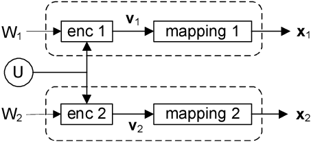
In this subsection we derive the achievable rate region for the interference channel. We prove that the region ℝIC​(πIC−I){\mathbb{R}}_{\rm IC}(\pi_{\rm IC-I}) is achievable. The coding structure for the IC-CM is illustrated in Fig. 6. We employ an auxiliary random variable UU in the sense of Han-Kobayashi [21] and two equivocation codebooks (stochastic encoders), one for each message W1W_{1} and W2W_{2}. Encoder tt maps 𝐯t\mathbf{v}_{t} into a channel input 𝐱t\mathbf{x}_{t}. More precisely, the random code generation is as follows.

Fix P⁡(u)P(u), P⁡(v1|u)P(v_{1}|u) and P⁡(v2|u)P(v_{2}|u), and

P(x1,x2|v1,v2)=P(x1|v1)P(x2|v2)P(x_{1},x_{2}|v_{1},v_{2})=P(x_{1}|v_{1})P(x_{2}|v_{2})

and let

R1′\displaystyle R^{\prime}_{1} ≜I(V1;Y2|V2,U)−ϵ1\displaystyle\triangleq I(V_{1};Y_{2}|V_{2},U)-\epsilon_{1} (52)
R2′\displaystyle R^{\prime}_{2} ≜I(V2;Y1|V1,U)−ϵ1\displaystyle\triangleq I(V_{2};Y_{1}|V_{1},U)-\epsilon_{1} (53)

where ϵ1>0\epsilon_{1}>0 and ϵ1\epsilon_{1} is small for sufficiently large nn.

Refer to caption

Fig. 6: Code construction for IC-CM
  • •

    [codebook generation] Randomly generate a typical sequence 𝐮\mathbf{u} with probability

    P⁡(𝐮)=∏i=1nP⁡(ui),P(\mathbf{u})=\prod_{i=1}^{n}P(u_{i}),

    and assume that both transmitters and receivers know the time-sharing sequence 𝐮\mathbf{u}.

    For transmitter tt, t=1,2t=1,2, generate Qt=2n⁡(Rt+Rt′)Q_{t}=2^{n(R_{t}+R^{\prime}_{t})} independent sequences 𝐯t\mathbf{v}_{t} each with probability

    P⁡(𝐯t|𝐮)=∏i=1nP⁡(vt,i|ui)P(\mathbf{v}_{t}|\mathbf{u})=\prod_{i=1}^{n}P(v_{t,i}|u_{i})

    and labeled as

    𝐯t​(wt,kt),wt∈{1,…,Mt},kt∈{1,…,Mt′}\displaystyle\mathbf{v}_{t}(w_{t},k_{t}),~w_{t}\in\{1,\ldots,M_{t}\},~k_{t}\in\{1,\ldots,M^{\prime}_{t}\} (54)

    where Mt=2n​RtM_{t}=2^{nR_{t}} and Mt′=2n​Rt′M^{\prime}_{t}=2^{nR^{\prime}_{t}}. Without loss of generality, MtM_{t}, Mt′M^{\prime}_{t}, and QtQ_{t} are assumed to be integers.

    Let

    𝒞t≜{𝐯t​(wt,kt), for all ​(wt,kt)}{\mathcal{C}}_{t}\triangleq\bigl\{\mathbf{v}_{t}(w_{t},k_{t}),\text{ for all }(w_{t},k_{t})\bigr\}

    be the codebook of Transmitter tt. Its wtw_{t}-th sub-codebook (bin)

    𝒞t​(wt)≜{𝐯t​(wt,kt), for ​kt=1,…,Mt′}{\mathcal{C}}_{t}(w_{t})\triangleq\{\mathbf{v}_{t}(w_{t},k_{t}),\text{ for }k_{t}=1,\ldots,M^{\prime}_{t}\bigr\}

    follows the partitioning in (54).

  • •

    [encoding] To send a message pair

    (w1,w2)∈𝒲1×𝒲2,(w_{1},w_{2})\in{\mathcal{W}}_{1}\times{\mathcal{W}}_{2},

    each transmitter employs a stochastic encoder. Encoder tt randomly chooses an element 𝐯t​(wt,kt)\mathbf{v}_{t}(w_{t},k_{t}) from the sub-codebook 𝒞t​(wt){\mathcal{C}}_{t}(w_{t}). Transmitters generate the channel input sequences based on respective mappings P⁡(x1|v1)P(x_{1}|v_{1}) and P⁡(x2|v2)P(x_{2}|v_{2}).

  • •

    [decoding] Given a typical sequence 𝐮\mathbf{u}, let Aϵ(n)​(PVt,Yt|U)A^{(n)}_{\epsilon}(P_{V_{t},Y_{t}|U}) denote the set of jointly typical sequences 𝐯t\mathbf{v}_{t} and 𝐲t\mathbf{y}_{t} with respect to P⁡(vt,yt|u)P(v_{t},y_{t}|u) [5]. Decoder tt chooses wtw_{t} so that

    (𝐯t​(wt,kt),𝐲t)∈Aϵ(n)​(PVt,Yt|U)(\mathbf{v}_{t}(w_{t},k_{t}),\mathbf{y}_{t})\in A^{(n)}_{\epsilon}(P_{V_{t},Y_{t}|U})

    when such wtw_{t} exists and and is unique; otherwise, an error is declared.

V-A1 Error Probability Analysis

To bound the probability of error, we define the event

Et(wt,kt)≜{(𝐯t(wt,kt),𝐲t|𝐮)∈Aϵ(n)(PVt,Yt|U)}.\displaystyle E_{t}(w_{t},k_{t})\triangleq\{(\mathbf{v}_{t}(w_{t},k_{t}),\mathbf{y}_{t}|\mathbf{u})\in A^{(n)}_{\epsilon}(P_{V_{t},Y_{t}|U})\}.

Without loss of generality, we can assume that transmitter 11 sends the message w1=1w_{1}=1 associated with the codeword 𝐯1​(1,1)\mathbf{v}_{1}(1,1), and define the corresponding event

K1≜{𝐯1​(1,1)​sent}.\displaystyle K_{1}\triangleq\{\mathbf{v}_{1}(1,1)~\text{sent}\}.

The union bound on the error probability of receiver 11 is as follows

Pe,1(n)\displaystyle P_{e,1}^{(n)} ≤P⁡{⋂k1E1c​(1,k1)|K1}+∑w1≠1,k1P⁡{E1​(w1,k1)|K1}\displaystyle\leq P\left\{\bigcap_{k_{1}}E_{1}^{c}(1,k_{1})\Big|K_{1}\right\}+\sum_{w_{1}\neq 1,\,k_{1}}P\{E_{1}(w_{1},k_{1})|K_{1}\}
≤P⁡{E1c​(1,1)|K1}+∑w1≠1,k1P⁡{E1​(w1,k1)|K1}\displaystyle\leq P\{E_{1}^{c}(1,1)|K_{1}\}+\sum_{w_{1}\neq 1,\,k_{1}}P\{E_{1}(w_{1},k_{1})|K_{1}\}

where E1c​(1,k1)E_{1}^{c}(1,k_{1}) denotes the event

{(𝐯1(1,k1),𝐲1)∉Aϵ(n)(PV1,Y1|U)}.\{(\mathbf{v}_{1}(1,k_{1}),\mathbf{y}_{1})\notin A^{(n)}_{\epsilon}(P_{V_{1},Y_{1}|U})\}.

Following the joint asymptotic equipartition property (AEP) [5], we have

P⁡{E1c​(1,1)|K1}≤ϵ,\displaystyle P\{E_{1}^{c}(1,1)|K_{1}\}\leq\epsilon,

and, for w1≠1w_{1}\neq 1,

P⁡{E1​(w1,k1)|K1}\displaystyle P\{E_{1}(w_{1},k_{1})|K_{1}\} ≤2−n⁡[I⁡(V1;Y1|U)−ϵ].\displaystyle\leq 2^{-n[I(V_{1};Y_{1}|U)-\epsilon]}.

Hence, we can bound the probability of error as

Pe,1(n)\displaystyle P_{e,1}^{(n)} ≤ϵ+Q1​2−n⁡[I⁡(V1;Y1|U)−ϵ]\displaystyle\leq\epsilon+Q_{1}2^{-n[I(V_{1};Y_{1}|U)-\epsilon]}
=ϵ+2n⁡(R1+R1′)​ 2−n⁡[I⁡(V1;Y1|U)−ϵ]\displaystyle=\epsilon+2^{n(R_{1}+R^{\prime}_{1})}\,2^{-n[I(V_{1};Y_{1}|U)-\epsilon]}

So, if

R1+R1′<I⁡(V1;Y1|U),R_{1}+R^{\prime}_{1}<I(V_{1};Y_{1}|U),

then for any ϵ0>0\epsilon_{0}>0, Pe,1(n)≤ϵ0P_{e,1}^{(n)}\leq\epsilon_{0} for sufficiently large nn. Similarly, for receiver 22, if

R2+R2′<I⁡(V2;Y2|U),R_{2}+R^{\prime}_{2}<I(V_{2};Y_{2}|U),

then Pe,2(n)≤ϵ0P_{e,2}^{(n)}\leq\epsilon_{0} for sufficiently large nn. Hence, Pe(n)≤ϵ0P^{(n)}_{e}\leq\epsilon_{0} as long as the rate pair (R1,R2)∈ℝIC​(πIC−I)(R_{1},R_{2})\in{\mathbb{R}}_{\rm IC}(\pi_{\rm IC-I}).

V-A2 Equivocation Calculation

To show that (5a) holds, we consider the following equivocation lower bound

H⁡(W1|𝐘2)\displaystyle H(W_{1}|\mathbf{Y}_{2}) ≥H⁡(W1|𝐘2,𝐕2,𝐔)\displaystyle\geq H(W_{1}|\mathbf{Y}_{2},\mathbf{V}_{2},\mathbf{U}) (55)

where inequality (55) is due to the fact that conditioning reduces entropy. By applying the entropy chain rule [5], (55) can be expanded as follows

H⁡(W1CLOSE\displaystyle H(W_{1} |𝐘2)\displaystyle|\mathbf{Y}_{2})
≥H(W1,𝐘2|𝐕2,𝐔)−H(𝐘2|𝐕2,𝐔)\displaystyle\geq H(W_{1},\mathbf{Y}_{2}|\mathbf{V}_{2},\mathbf{U})-H(\mathbf{Y}_{2}|\mathbf{V}_{2},\mathbf{U})
=H(W1,𝐕1,𝐘2|𝐕2,𝐔)\displaystyle=H(W_{1},\mathbf{V}_{1},\mathbf{Y}_{2}|\mathbf{V}_{2},\mathbf{U})
−H⁡(𝐕1|𝐘2,𝐕2,𝐔,W1)−H⁡(𝐘2|𝐕2,𝐔)\displaystyle\quad-H(\mathbf{V}_{1}|\mathbf{Y}_{2},\mathbf{V}_{2},\mathbf{U},W_{1})-H(\mathbf{Y}_{2}|\mathbf{V}_{2},\mathbf{U})
=H(W1,𝐕1|𝐕2,𝐔)−H(𝐕1|𝐘2,𝐕2,𝐔,W1)\displaystyle=H(W_{1},\mathbf{V}_{1}|\mathbf{V}_{2},\mathbf{U})-H(\mathbf{V}_{1}|\mathbf{Y}_{2},\mathbf{V}_{2},\mathbf{U},W_{1})
−H⁡(𝐘2|𝐕2,𝐔)+H⁡(𝐘2|𝐕1,𝐕2,𝐔,W1).\displaystyle\quad-H(\mathbf{Y}_{2}|\mathbf{V}_{2},\mathbf{U})+H(\mathbf{Y}_{2}|\mathbf{V}_{1},\mathbf{V}_{2},\mathbf{U},W_{1}). (56)

Based on functional dependence graphs [27] and the random code construction, we can show that the following is a Markov chain

W1\displaystyle W_{1} →(𝐕1,𝐕2,𝐔)→𝐘2\displaystyle\rightarrow(\mathbf{V}_{1},\mathbf{V}_{2},\mathbf{U})\rightarrow\mathbf{Y}_{2}

which yields

I(W1;𝐘2|𝐕1,𝐕2,𝐔)\displaystyle I(W_{1};\mathbf{Y}_{2}|\mathbf{V}_{1},\mathbf{V}_{2},\mathbf{U}) =0.\displaystyle=0. (57)

Hence, by using (56) and (57), we obtain

H⁡(W1|𝐘2)\displaystyle H(W_{1}|\mathbf{Y}_{2}) ≥H(W1,𝐕1|𝐕2,𝐔)−H(𝐕1|𝐘2,𝐕2,𝐔,W1)\displaystyle\geq H(W_{1},\mathbf{V}_{1}|\mathbf{V}_{2},\mathbf{U})-H(\mathbf{V}_{1}|\mathbf{Y}_{2},\mathbf{V}_{2},\mathbf{U},W_{1})
−H⁡(𝐘2|𝐕2,𝐔)+H⁡(𝐘2|𝐕1,𝐕2,𝐔)\displaystyle\quad-H(\mathbf{Y}_{2}|\mathbf{V}_{2},\mathbf{U})+H(\mathbf{Y}_{2}|\mathbf{V}_{1},\mathbf{V}_{2},\mathbf{U})
=H(W1,𝐕1|𝐕2,𝐔)−H(𝐕1|𝐘2,𝐕2,𝐔,W1)\displaystyle=H(W_{1},\mathbf{V}_{1}|\mathbf{V}_{2},\mathbf{U})-H(\mathbf{V}_{1}|\mathbf{Y}_{2},\mathbf{V}_{2},\mathbf{U},W_{1})
−I(𝐕1;𝐘2|𝐕2,𝐔)\displaystyle\quad-I(\mathbf{V}_{1};\mathbf{Y}_{2}|\mathbf{V}_{2},\mathbf{U})
≥H⁡(𝐕1|𝐕2,𝐔)−H⁡(𝐕1|𝐘2,𝐕2,𝐔,W1)\displaystyle\geq H(\mathbf{V}_{1}|\mathbf{V}_{2},\mathbf{U})-H(\mathbf{V}_{1}|\mathbf{Y}_{2},\mathbf{V}_{2},\mathbf{U},W_{1})
−I(𝐕1;𝐘2|𝐕2,𝐔).\displaystyle\quad-I(\mathbf{V}_{1};\mathbf{Y}_{2}|\mathbf{V}_{2},\mathbf{U}). (58)

We consider the first term in (58). Note that given 𝐔=𝐮\mathbf{U}=\mathbf{u}, 𝐕1\mathbf{V}_{1} and 𝐕2\mathbf{V}_{2} are independent and 𝐕1\mathbf{V}_{1} has Q1Q_{1} possible values with equal probability. Hence,

H⁡(𝐕1|𝐔,𝐕2)\displaystyle H(\mathbf{V}_{1}|\mathbf{U},\mathbf{V}_{2}) =H⁡(𝐕1|𝐔)\displaystyle=H(\mathbf{V}_{1}|\mathbf{U})
=log⁡Q1\displaystyle=\log Q_{1}
=n⁡(R1+R1′).\displaystyle=n(R_{1}+R^{\prime}_{1}). (59)

We next show that H⁡(𝐕1|𝐘2,𝐕2,𝐔,W1)≤n​ϵ2H(\mathbf{V}_{1}|\mathbf{Y}_{2},\mathbf{V}_{2},\mathbf{U},W_{1})\leq n\epsilon_{2}, where ϵ2\epsilon_{2} is small for sufficiently large nn. In order to calculate the conditional entropy H⁡(𝐕1|𝐘2,𝐕2,𝐔,W1)H(\mathbf{V}_{1}|\mathbf{Y}_{2},\mathbf{V}_{2},\mathbf{U},W_{1}), we consider the following situation. We fix W1=w1W_{1}=w_{1}, and assume that transmitter 11 transmits a codeword 𝐯1​(w1,k1)∈𝒞1​(w1)\mathbf{v}_{1}(w_{1},k_{1})\in{\mathcal{C}}_{1}(w_{1}), for 1≤k1≤M1′1\leq k_{1}\leq M^{\prime}_{1}, and that receiver 22 knows the sequences 𝐕2=𝐯2\mathbf{V}_{2}=\mathbf{v}_{2} and 𝐔=𝐮\mathbf{U}=\mathbf{u}. Given index W1=w1W_{1}=w_{1}, receiver 22 decodes the codeword 𝐯1​(w1,k1)\mathbf{v}_{1}(w_{1},k_{1}) based on the received sequence 𝐲2\mathbf{y}_{2}. Let λ⁡(w1)\lambda(w_{1}) denote the average probability of error of decoding the index k1k_{1} at receiver 22. Based on joint typicality [5, Chapter 8], we have the following lemma.

Lemma 2

λ⁡(w1)≤ϵ0\lambda(w_{1})\leq\epsilon_{0} for sufficiently large nn.

Proof:

We provide the proof in the Appendix. ∎Fano’s inequality implies that

1n​H​(𝐕1|𝐘2,𝐕2,𝐔,W1=w1)\displaystyle\frac{1}{n}H(\mathbf{V}_{1}|\mathbf{Y}_{2},\mathbf{V}_{2},\mathbf{U},W_{1}=w_{1}) ≤1n​[1+λ⁡(w1)​log⁡M1′]\displaystyle\leq\frac{1}{n}[1+\lambda(w_{1})\log M^{\prime}_{1}]
≤1n+ϵ0​I​(V1;Y2|U)\displaystyle\leq\frac{1}{n}+\epsilon_{0}I(V_{1};Y_{2}|U)
≜ϵ2\displaystyle\triangleq\epsilon_{2} (60)

where the second inequality follows from Lemma 2 and (52). Consequently,

1n​H\displaystyle\frac{1}{n}H (𝐕1|𝐘2,𝐕2,𝐔,W1)\displaystyle(\mathbf{V}_{1}|\mathbf{Y}_{2},\mathbf{V}_{2},\mathbf{U},W_{1})
=1n​∑w1∈𝒲1P⁡(W1=w1)​H​(𝐕1|𝐘2,𝐕2,𝐔,W1=w1)\displaystyle=\frac{1}{n}\sum_{w_{1}\in{\mathcal{W}}_{1}}P(W_{1}=w_{1})H(\mathbf{V}_{1}|\mathbf{Y}_{2},\mathbf{V}_{2},\mathbf{U},W_{1}=w_{1})
≤ϵ2.\displaystyle\leq\epsilon_{2}. (61)

Finally, the third term in (58) can be bounded based on the following lemma.

Lemma 3
I(𝐕1;𝐘2|𝐕2,𝐔)≤nI(V1;Y2|V2,U)+nϵ3\displaystyle I(\mathbf{V}_{1};\mathbf{Y}_{2}|\mathbf{V}_{2},\mathbf{U})\leq nI(V_{1};Y_{2}|V_{2},U)+n\epsilon_{3} (62)

where ϵ3\epsilon_{3} is small for sufficiently large nn.

Proof:

We provide the proof in the Appendix. ∎

By using (59), (61), and (62), we can rewrite (58) as

1nH(W1|𝐘2)≥R1+R1′−I(V1;Y2|V2,U)−ϵ2−ϵ3.\displaystyle\frac{1}{n}H(W_{1}|\mathbf{Y}_{2})\geq R_{1}+R^{\prime}_{1}-I(V_{1};Y_{2}|V_{2},U)-\epsilon_{2}-\epsilon_{3}.

By the definition of R1′R^{\prime}_{1} (52), we have

R1−1n​H​(W1|𝐘2,𝐗2,W2)≤ϵ4\displaystyle R_{1}-\frac{1}{n}H(W_{1}|\mathbf{Y}_{2},\mathbf{X}_{2},W_{2})\leq\epsilon_{4} (63)

where ϵ4≜ϵ1+ϵ2+ϵ3\epsilon_{4}\triangleq\epsilon_{1}+\epsilon_{2}+\epsilon_{3}, and, thus, the security condition (5a) is satisfied. Following the same approach, we can prove that (5b) is satisfied.

V-B Broadcast Channel with Confidential Messages

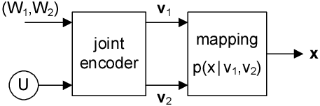
We next prove Theorem 4 based on the double-binning scheme which combines the Gel’fand-Pinsker binning [23] and the random binning. In this subsection we redefine the parameters R1R_{1}, R2R_{2}, R1′R^{\prime}_{1}, R2′R^{\prime}_{2}, Q1Q_{1}, Q2Q_{2}, M1M_{1}, and M2M_{2}. The coding structure for the BC-CM is shown in Fig. 7.
Refer to caption

Fig. 7: Code construction for BC-CM

We employ a joint encoder to generate two equivocation codewords 𝐯1\mathbf{v}_{1} and 𝐯2\mathbf{v}_{2}, one for each message W1W_{1} and W2W_{2}. The equivocation codewords are mapped into the channel input 𝐱\mathbf{x}. The details of random code generation are as follows.

We fix P⁡(u)P(u), P⁡(v1|u)P(v_{1}|u) and P⁡(v2|u)P(v_{2}|u), as well as P⁡(x|v1,v2)P(x|v_{1},v_{2}). Let 0≤α≤10\leq\alpha\leq 1,

R1′\displaystyle R^{\prime}_{1} ≜I(V1;Y2|V2,U)−ϵ1′\displaystyle\triangleq I(V_{1};Y_{2}|V_{2},U)-\epsilon^{\prime}_{1}
R2′\displaystyle R^{\prime}_{2} ≜I(V2;Y1|V1,U)−ϵ1′\displaystyle\triangleq I(V_{2};Y_{1}|V_{1},U)-\epsilon^{\prime}_{1} (64)

and

R†≜I⁡(V1;V2|U)+ϵ1′\displaystyle R^{{\dagger}}\triangleq I(V_{1};V_{2}|U)+\epsilon^{\prime}_{1} (65)

where ϵ1′>0\epsilon^{\prime}_{1}>0 and ϵ1′\epsilon^{\prime}_{1} is small for sufficiently large nn.

  • •

    [codebook generation] We generate randomly a typical sequence 𝐮\mathbf{u} with probability

    P⁡(𝐮)=∏i=1nP⁡(ui)P(\mathbf{u})=\prod_{i=1}^{n}P(u_{i})

    and assume that both the transmitter and the receivers know the sequence 𝐮\mathbf{u}.

    We generate Qt=2n⁡(Rt+Rt′+R†)Q_{t}=2^{n(R_{t}+R^{\prime}_{t}+R^{{\dagger}})} independent sequences 𝐯t\mathbf{v}_{t} each with probability

    P⁡(𝐯t|𝐮)=∏i=1nP⁡(vt,i|ui)P(\mathbf{v}_{t}|\mathbf{u})=\prod_{i=1}^{n}P(v_{t,i}|u_{i})

    and label them

    𝐯t​(wt,st,kt),\displaystyle\mathbf{v}_{t}(w_{t},s_{t},k_{t}), wt∈{1,…,Mt},st∈{1,…,Jt},\displaystyle\quad w_{t}\in\{1,\ldots,M_{t}\},~s_{t}\in\{1,\ldots,J_{t}\},
    and​kt∈{1,…,Gt}.\displaystyle\quad\text{and}~k_{t}\in\{1,\ldots,G_{t}\}. (66)

    where Mt=2n​RtM_{t}=2^{nR_{t}}, Jt=2n​Rt′,J_{t}=2^{nR^{\prime}_{t}}, and Gt=2n​R†G_{t}=2^{nR^{{\dagger}}}. Without loss of generality QtQ_{t}, MtM_{t}, JtJ_{t}, and GtG_{t} are considered to be integers.

    Refer to caption

    Fig. 8: Double binning

    Let

    𝒞t≜{𝐯t​(wt,st,kt), for all ​(wt,st,kt)}{\mathcal{C}}_{t}\triangleq\bigl\{\mathbf{v}_{t}(w_{t},s_{t},k_{t}),\text{ for all }(w_{t},s_{t},k_{t})\bigr\}

    denote the transmitter tt codebook. Based on the labeling in (66), the codebook 𝒞t{\mathcal{C}}_{t} is partitioned into MtM_{t} bins, and the wtw_{t}-th bin is

    𝒞t​(wt)\displaystyle{\mathcal{C}}_{t}(w_{t}) ≜{𝐯t(wt,st,kt), for st∈{1,…,Jt}\displaystyle\triangleq\{\mathbf{v}_{t}(w_{t},s_{t},k_{t}),\text{ for }s_{t}\in\{1,\ldots,J_{t}\}
     and ​kt∈{1,…,Gt}.\displaystyle\qquad\text{ and }k_{t}\in\{1,\ldots,G_{t}\bigr\}.

    Furthermore, each bin 𝒞t​(wt){\mathcal{C}}_{t}(w_{t}) is divided into JtJ_{t} sub-bins, and the (wt,st)(w_{t},s_{t})-th sub-bin is

    𝒞t​(wt,st)\displaystyle{\mathcal{C}}_{t}(w_{t},s_{t}) ≜{𝐯t​(wt,st,kt), for ​kt∈{1,…,Gt}}.\displaystyle\triangleq\bigl\{\mathbf{v}_{t}(w_{t},s_{t},k_{t}),\text{ for }k_{t}\in\{1,\ldots,G_{t}\}\bigr\}.

    The double binning structure for 𝐯t\mathbf{v}_{t} sequences is shown in Fig. 8.

  • •

    [encoding] To send the message pair (w1,w2)∈𝒲1×𝒲2(w_{1},w_{2})\in{\mathcal{W}}_{1}\times{\mathcal{W}}_{2}, the transmitter employs a stochastic encoder. We randomly choose a sub-bin 𝒞t​(wt,st){\mathcal{C}}_{t}(w_{t},s_{t}) from the bin 𝒞t​(wt){\mathcal{C}}_{t}(w_{t}), for t=1,2t=1,2. Next, we select a pair (k1,k2)(k_{1},k_{2}) so that

    (𝐯1​(w1,s1,k1),𝐯2​(w2,s2,k2))∈Aϵ(n)​(PV1,V2|U),\bigl(\mathbf{v}_{1}(w_{1},s_{1},k_{1}),\mathbf{v}_{2}(w_{2},s_{2},k_{2})\bigr)\in A^{(n)}_{\epsilon}(P_{V_{1},V_{2}|U}),

    where Aϵ(n)​(PV1,V2|U)A^{(n)}_{\epsilon}(P_{V_{1},V_{2}|U}) denotes, for a given typical sequence 𝐮\mathbf{u}, the set of jointly typical sequences 𝐯1\mathbf{v}_{1} and 𝐯2\mathbf{v}_{2} with respect to P⁡(v1,v2|u)P(v_{1},v_{2}|u). If there are more than one such pairs, then we randomly select one. We generate the channel input sequence 𝐱\mathbf{x} according to the mapping P⁡(x|v1,v2)P(x|v_{1},v_{2}).

  • •

    [decoding] For a given typical sequence 𝐮\mathbf{u}, let Aϵ(n)​(PVt,Yt|U)A^{(n)}_{\epsilon}(P_{V_{t},Y_{t}|U}) denote the set of jointly typical sequences 𝐯t\mathbf{v}_{t} and 𝐲t\mathbf{y}_{t} with respect to P⁡(vt,yt|u)P(v_{t},y_{t}|u). Decoder tt chooses wtw_{t} so that (𝐯t​(wt,st,kt),𝐲t)∈Aϵ(n)​(PVt,Yt|U)(\mathbf{v}_{t}(w_{t},s_{t},k_{t}),\mathbf{y}_{t})\in A^{(n)}_{\epsilon}(P_{V_{t},Y_{t}|U}) if such wtw_{t} exists and is unique; otherwise, an error is declared.

V-B1 Error Probability Analysis

Without loss of generality, we assume that the message pair is (w1=1,w2=1)(w_{1}=1,w_{2}=1) and that s1=s2=1s_{1}=s_{2}=1. First, we consider the error event TT that the encoder can not find an appropriate jointly typical pair, i.e.,

T\displaystyle T ≜{(𝐯1(1,1,k1),𝐯2(1,1,k2))∉Aϵ(n)(PV1,V2|U),\displaystyle\triangleq\{\bigl(\mathbf{v}_{1}(1,1,k_{1}),\mathbf{v}_{2}(1,1,k_{2})\bigr)\notin A^{(n)}_{\epsilon}(P_{V_{1},V_{2}|U}),
 for st=1,…,Jt,kt=1,…,Gt, and t=1,2}.\displaystyle\qquad\text{ for }s_{t}=1,\ldots,J_{t},~k_{t}=1,\ldots,G_{t},\text{ and }t=1,2\}.

The definition of R†R^{{\dagger}} in (65) implies that

R†>I⁡(V1;V2|U).\displaystyle R^{{\dagger}}>I(V_{1};V_{2}|U). (67)

Hence, following the approach of [28], we have that

P​{T}≤δ3\displaystyle P\{T\}\leq\delta_{3} (68)

where δ3>0\delta_{3}>0 and δ3\delta_{3} is small for sufficiently large nn. In other words, the encoding is successful with probability close to 11 as long as nn is large.

In the following, we assume that (v1​(1,1,1),v2​(1,1,1))(v_{1}(1,1,1),v_{2}(1,1,1)) is sent and define the event

K2≜{(𝐯1(1,1,1),𝐯2(1,1,1))∈Aϵ(n)(PV1,V2|U)}.\displaystyle K_{2}\triangleq\{(\mathbf{v}_{1}(1,1,1),\mathbf{v}_{2}(1,1,1))\in A^{(n)}_{\epsilon}(P_{V_{1},V_{2}|U})\}.

Now, the error probability at receiver 11 is bounded as follows

Pe,1(n)\displaystyle P_{e,1}^{(n)} ≤P{T}+(1−P{T})[P{⋂s1,k1E1c(1,s1,k1)|K2}\displaystyle\leq P\{T\}+(1-P\{T\})\Biggl[P\Biggl\{\bigcap_{s_{1},k_{1}}E_{1}^{c}(1,s_{1},k_{1})\Big|K_{2}\Biggr\}
+∑w1≠1∑s1,k1P{E1(w1,s1,k1)|K2}]\displaystyle\qquad+\sum_{w_{1}\neq 1}\sum_{s_{1},k_{1}}P\{E_{1}(w_{1},s_{1},k_{1})|K_{2}\}\Biggr]
≤P⁡{T}+P⁡{E1c​(1,1,1)|K2}\displaystyle\leq P\{T\}+P\{E_{1}^{c}(1,1,1)|K_{2}\}
+∑w1≠1∑s1,k1P{E1(w1,s1,k1)|K2}\displaystyle\qquad+\sum_{w_{1}\neq 1}\sum_{s_{1},k_{1}}P\{E_{1}(w_{1},s_{1},k_{1})|K_{2}\}

where

Et(wt,st,kt)={(𝐯t(wt,st,kt),𝐲t)∈Aϵ(n)(PVt,Yt|U)}.E_{t}(w_{t},s_{t},k_{t})=\{(\mathbf{v}_{t}(w_{t},s_{t},k_{t}),\mathbf{y}_{t})\in A^{(n)}_{\epsilon}(P_{V_{t},Y_{t}|U})\}.

Joint typicality [5, Chapter 14] implies that

P⁡{E1c​(1,1,1)|K2}\displaystyle P\{E_{1}^{c}(1,1,1)|K_{2}\} ≤ϵ,\displaystyle\leq\epsilon,
P⁡{E1​(w1,s1,k1)|K2}\displaystyle P\{E_{1}(w_{1},s_{1},k_{1})|K_{2}\} ≤2−n⁡[I⁡(V1;Y1|U)−ϵ]for ​w1≠1.\displaystyle\leq 2^{-n[I(V_{1};Y_{1}|U)-\epsilon]}\quad\text{for }w_{1}\neq 1.

Hence, we can bound the probability of error as

Pe,1(n)\displaystyle P_{e,1}^{(n)} ≤δ3+ϵ+Q1​2−n⁡[I⁡(V1;Y1|U)−ϵ]\displaystyle\leq\delta_{3}+\epsilon+Q_{1}2^{-n[I(V_{1};Y_{1}|U)-\epsilon]}
=δ3+ϵ+2n⁡(R1+R1′+R†)​ 2−n⁡[I⁡(V1;Y1|U)−ϵ]\displaystyle=\delta_{3}+\epsilon+2^{n(R_{1}+R^{\prime}_{1}+R^{{\dagger}})}\,2^{-n[I(V_{1};Y_{1}|U)-\epsilon]} (69)

So, if

R1+R1′+R†<I⁡(V1;Y1|U),\displaystyle R_{1}+R^{\prime}_{1}+R^{{\dagger}}<I(V_{1};Y_{1}|U), (70)

then for any ϵ0>0\epsilon_{0}>0, Pe,1(n)≤ϵ0P_{e,1}^{(n)}\leq\epsilon_{0} for sufficiently large nn. Similarly, for receiver 22, if

R2+R2′+R†<I⁡(V2;Y2|U),\displaystyle R_{2}+R^{\prime}_{2}+R^{{\dagger}}<I(V_{2};Y_{2}|U), (71)

then Pe,2(n)≤ϵ0P_{e,2}^{(n)}\leq\epsilon_{0} for sufficiently large nn. Hence, (2), (64), (65), (70), and (71) imply that Pe(n)≤ϵ0P^{(n)}_{e}\leq\epsilon_{0} as long as the rate pair (R1,R2)∈ℝBC​(πBC).(R_{1},R_{2})\in{\mathbb{R}}_{\rm BC}(\pi_{\rm BC}).

V-B2 Equivocation Calculation

We next prove that the secrecy requirement (5a) holds for BC-CM. Following the same approach as (55)–(58), we have

H⁡(W1|𝐘2)\displaystyle H(W_{1}|\mathbf{Y}_{2}) ≥H⁡(𝐕1|𝐕2,𝐔)−H⁡(𝐕1|𝐘2,𝐕2,𝐔,W1)\displaystyle\geq H(\mathbf{V}_{1}|\mathbf{V}_{2},\mathbf{U})-H(\mathbf{V}_{1}|\mathbf{Y}_{2},\mathbf{V}_{2},\mathbf{U},W_{1})
−I(𝐕1;𝐘2|𝐕2,𝐔).\displaystyle\qquad-I(\mathbf{V}_{1};\mathbf{Y}_{2}|\mathbf{V}_{2},\mathbf{U}). (72)

Consider the first term in (72)

H⁡(𝐕1|𝐔,𝐕2)\displaystyle H(\mathbf{V}_{1}|\mathbf{U},\mathbf{V}_{2}) =H⁡(𝐕1|𝐔)−I⁡(𝐕1;𝐕2|𝐔).\displaystyle=H(\mathbf{V}_{1}|\mathbf{U})-I(\mathbf{V}_{1};\mathbf{V}_{2}|\mathbf{U}).

Note that given 𝐔=𝐮\mathbf{U}=\mathbf{u}, 𝐕1\mathbf{V}_{1} attains Q1Q_{1} possible values with equal probability. Hence, we have H⁡(𝐕1|𝐔)=log⁡Q1.H(\mathbf{V}_{1}|\mathbf{U})=\log Q_{1}. Using the same approach as in Lemma 3, we can obtain

I⁡(𝐕1;𝐕2|𝐔)\displaystyle I(\mathbf{V}_{1};\mathbf{V}_{2}|\mathbf{U}) ≤n​I​(V1;V2|U)+n​ϵ2′.\displaystyle\leq nI(V_{1};V_{2}|U)+n\epsilon^{\prime}_{2}. (73)

Hence, by the definition of R†R^{{\dagger}} in (65), we have

H⁡(𝐕1|𝐔,𝐕2)\displaystyle H(\mathbf{V}_{1}|\mathbf{U},\mathbf{V}_{2}) =log⁡Q1−I⁡(𝐕1;𝐕2|𝐔)\displaystyle=\log Q_{1}-I(\mathbf{V}_{1};\mathbf{V}_{2}|\mathbf{U})
≥n⁡(R1+R1′+R†)−n​I​(V1;V2|U)−n​ϵ2′\displaystyle\geq n(R_{1}+R^{\prime}_{1}+R^{{\dagger}})-nI(V_{1};V_{2}|U)-n\epsilon^{\prime}_{2}
≥n⁡(R1+R1′−ϵ2′).\displaystyle\geq n(R_{1}+R^{\prime}_{1}-\epsilon^{\prime}_{2}). (74)

Following joint typicality [5], (61) implies

H⁡(𝐕1|𝐘2,𝐕2,𝐔,W1)≤n​ϵ3′H(\mathbf{V}_{1}|\mathbf{Y}_{2},\mathbf{V}_{2},\mathbf{U},W_{1})\leq n\epsilon^{\prime}_{3}

where ϵ3′\epsilon^{\prime}_{3} is small for sufficiently large nn. Applying Lemma 3, the third term in (72) can be bounded as

I(𝐕1;𝐘2|𝐕2,𝐔)\displaystyle I(\mathbf{V}_{1};\mathbf{Y}_{2}|\mathbf{V}_{2},\mathbf{U}) ≤nI(V1;Y2|V2,U)+nϵ4′\displaystyle\leq nI(V_{1};Y_{2}|V_{2},U)+n\epsilon^{\prime}_{4}
=n⁡(R1′+ϵ1′+ϵ4′)\displaystyle=n(R^{\prime}_{1}+\epsilon^{\prime}_{1}+\epsilon^{\prime}_{4}) (75)

where ϵ4′\epsilon^{\prime}_{4} is small for sufficiently large nn and the equality (75) follows from the definition (64). Hence, by using (73), (74), and (75), we can rewrite (72) as

1n​H​(W1|𝐘2)≥R1−ϵ5′\displaystyle\frac{1}{n}H(W_{1}|\mathbf{Y}_{2})\geq R_{1}-\epsilon^{\prime}_{5}

where ϵ5′≜ϵ1′+ϵ2′+ϵ3′+ϵ4′\epsilon^{\prime}_{5}\triangleq\epsilon^{\prime}_{1}+\epsilon^{\prime}_{2}+\epsilon^{\prime}_{3}+\epsilon^{\prime}_{4}, and thus the security condition (5a) is satisfied. Following the same approach, we can prove that (5b) also holds.

VI Conclusion

We derived the outer and the inner bounds on the capacity of the interference and broadcast channels with confidential messages. The obtained results offer insights into the two communication problems. The difference in the outer bound reflects the fact that the joint encoding at the transmitter can only be performed in the BC-CM whereas in the IC-CM, encoders offer independent channel inputs. The achievability proof suggests the code construction appropriate for these channel. We presented a special case of IC-CM for which the two bounds meet to describe the capacity region. We proposed and compared several transmission schemes for Gaussian interference channels under information-theoretic secrecy. In particular, the encoding scheme in which transmitters dedicate some of their power to create artificial noise was shown to outperform both time-sharing and simultaneous transmission of messages sent with the optimal power. However, constructing practical wiretap codes that can achieve the derived rates is a challenging problem. Code constructions for a binary-input Gaussian wiretap channel have recently been proposed in [29].

Proof:

(Lemma 1) By the definition of Δ1\Delta_{1}, we have

Δ1\displaystyle\Delta_{1} =I⁡(V1;Y1|U)−I⁡(V1;Y2|U)\displaystyle=I(V_{1};Y_{1}|U)-I(V_{1};Y_{2}|U)
=I(V1,V2;Y1|U)−I(V2;Y1|V1,U)\displaystyle=I(V_{1},V_{2};Y_{1}|U)-I(V_{2};Y_{1}|V_{1},U)
−I(V1,V2;Y2|U)+I(V2;Y2|V1,U).\displaystyle\qquad-I(V_{1},V_{2};Y_{2}|U)+I(V_{2};Y_{2}|V_{1},U). (76)

Similarly,

Δ2\displaystyle\Delta_{2} =I⁡(V2;Y2|U)−I⁡(V2;Y1|U)\displaystyle=I(V_{2};Y_{2}|U)-I(V_{2};Y_{1}|U)
=I(V1,V2;Y2|U)−I(V1;Y2|V2,U)\displaystyle=I(V_{1},V_{2};Y_{2}|U)-I(V_{1};Y_{2}|V_{2},U)
−I(V1,V2;Y2|U)+I(V1;Y1|V2,U).\displaystyle\qquad-I(V_{1},V_{2};Y_{2}|U)+I(V_{1};Y_{1}|V_{2},U). (77)

(76) and (77) imply that

Δ1+Δ2\displaystyle\Delta_{1}+\Delta_{2} =−I(V2;Y1|V1,U)+I(V2;Y2|V1,U)\displaystyle=-I(V_{2};Y_{1}|V_{1},U)+I(V_{2};Y_{2}|V_{1},U)
−I(V1;Y2|V2,U)+I(V1;Y1|V2,U)\displaystyle\qquad-I(V_{1};Y_{2}|V_{2},U)+I(V_{1};Y_{1}|V_{2},U)
=Θ2+Θ1.\displaystyle=\Theta_{2}+\Theta_{1}. (78)

Note that

2​(Δ1+Δ2)\displaystyle 2(\Delta_{1}+\Delta_{2}) =2​(Θ1+Θ2)\displaystyle=2(\Theta_{1}+\Theta_{2})
=(Δ1+Θ2)+(Δ2+Θ1)\displaystyle=(\Delta_{1}+\Theta_{2})+(\Delta_{2}+\Theta_{1})

Hence, min[Δ_1+Θ_2, Δ_2+Θ_1] ≤Δ_1+Δ_2 =Θ_1+Θ_2. We have the derived results. ∎

Proof:

(Lemma 2) For a given typical sequence pair (𝐯2,𝐮)(\mathbf{v}_{2},\mathbf{u}), let Aϵ(n)​(PV1,Y2|V2,U)A^{(n)}_{\epsilon}(P_{V_{1},Y_{2}|V_{2},U}) denote the set of jointly typical sequences 𝐯1\mathbf{v}_{1} and 𝐲2\mathbf{y}_{2} with respect to P(v1,y2|v2,u)P(v_{1},y_{2}|v_{2},u). For a given W1=w1W_{1}=w_{1}, decoder 22 chooses k1k_{1} so that (v_1(w_1,k_1), y_2)∈A^(n)_ϵ(P_V_1,Y_2—V_2,U) if such k1k_{1} exists and is unique; otherwise, an error is declared. Define the event

E^(k1)={(𝐯1(w1,k1),𝐲2)∈Aϵ(n)(PV1,Y2|V2,U)}.\displaystyle\hat{E}(k_{1})=\{(\mathbf{v}_{1}(w_{1},k_{1}),\mathbf{y}_{2})\in A^{(n)}_{\epsilon}(P_{V_{1},Y_{2}|V_{2},U})\}.

Without loss of generality, we assume that 𝐯1​(w1,k1=1)\mathbf{v}_{1}(w_{1},k_{1}=1) was sent, and define the event

K^1={𝐯1​(w1,1)​sent}.\displaystyle\hat{K}_{1}=\bigl\{\mathbf{v}_{1}(w_{1},1)~\text{sent}\bigr\}.

Hence

λ⁡(w1)\displaystyle\lambda(w_{1}) ≤P⁡{E^c​(k1=1)|K^1}+∑k1≠1P⁡{E^​(k1)|K^1}\displaystyle\leq P\{\hat{E}^{c}(k_{1}=1)|\hat{K}_{1}\}+\sum_{k_{1}\neq 1}P\{\hat{E}(k_{1})|\hat{K}_{1}\}

where E^c​(k1=1)\hat{E}^{c}(k_{1}=1) denotes the event {(v_1(w_1,1), y_2)∉A^(n)_ϵ(P_V_1,Y_2—V_2,U)}. Following the joint AEP [5], we have

P⁡{E^c​(k1=1)|K^1}≤ϵ,\displaystyle P\{\hat{E}^{c}(k_{1}=1)|\hat{K}_{1}\}\leq\epsilon,

and, for k1≠1k_{1}\neq 1,

P{E^(k1)|K^1}≤2−n[I(V1;Y2|V2,U)−ϵ].\displaystyle P\{\hat{E}(k_{1})|\hat{K}_{1}\}\leq 2^{-n[I(V_{1};Y_{2}|V_{2},U)-\epsilon]}.

Now, we can bound the probability of error as

λ⁡(w1)\displaystyle\lambda(w_{1}) ≤ϵ+M′12−n[I(V1;Y2|V2,U)−ϵ]\displaystyle\leq\epsilon+M^{\prime}_{1}2^{-n[I(V_{1};Y_{2}|V_{2},U)-\epsilon]}
≤ϵ+2n​R1′ 2−n[I(V1;Y2|V2,U)−ϵ].\displaystyle\leq\epsilon+2^{nR^{\prime}_{1}}\,2^{-n[I(V_{1};Y_{2}|V_{2},U)-\epsilon]}.

Note that R1′=I(V1;Y2|V2,U)−ϵ1R^{\prime}_{1}=I(V_{1};Y_{2}|V_{2},U)-\epsilon_{1}. Hence, by choosing ϵ1>ϵ\epsilon_{1}>\epsilon, we have

λ⁡(w1)≤ϵ0\displaystyle\lambda(w_{1})\leq\epsilon_{0}

where ϵ0\epsilon_{0} is small for sufficiently large nn. ∎

Proof:

(Lemma 3) Let Aϵ(n)​(PU,V1,V2,Y2)A^{(n)}_{\epsilon}(P_{U,V_{1},V_{2},Y_{2}}) denote the set of typical sequences (𝐮,𝐯1,𝐯2,𝐲2)(\mathbf{u},\mathbf{v}_{1},\mathbf{v}_{2},\mathbf{y}_{2}) with respect to P⁡(u,v1,v2,y2)P(u,v_{1},v_{2},y_{2}), and

μ⁡(𝐮,𝐯1CLOSE,\displaystyle\mu(\mathbf{u},\mathbf{v}_{1}, 𝐯2,𝐲2)={1,(𝐮,𝐯1,𝐯2,𝐲2)∉Aϵ(n)​(PU,V1,V2,Y2)0,otherwise\displaystyle\mathbf{v}_{2},\mathbf{y}_{2})=\left\{\begin{array}[]{ll}1,&(\mathbf{u},\mathbf{v}_{1},\mathbf{v}_{2},\mathbf{y}_{2})\notin A^{(n)}_{\epsilon}(P_{U,V_{1},V_{2},Y_{2}})\\ 0,&\hbox{otherwise}\end{array}\right.

be the corresponding indicator function.

We expand I(𝐕1;𝐘2|𝐕2,𝐔)I(\mathbf{V}_{1};\mathbf{Y}_{2}|\mathbf{V}_{2},\mathbf{U}) as

I(𝐕1;𝐘2|𝐕2,𝐔)\displaystyle I(\mathbf{V}_{1};\mathbf{Y}_{2}|\mathbf{V}_{2},\mathbf{U}) ≤I(𝐕1,μ;𝐘2|𝐕2,𝐔)\displaystyle\leq I(\mathbf{V}_{1},\mu;\mathbf{Y}_{2}|\mathbf{V}_{2},\mathbf{U})
=I(𝐕1;𝐘2|𝐕2,𝐔,μ)+I(μ;𝐘2|𝐕2,𝐔)\displaystyle=I(\mathbf{V}_{1};\mathbf{Y}_{2}|\mathbf{V}_{2},\mathbf{U},\mu)+I(\mu;\mathbf{Y}_{2}|\mathbf{V}_{2},\mathbf{U})
=∑j=01P(μ=j)I(𝐕1;𝐘2|𝐕2,𝐔,μ=j)\displaystyle=\sum_{j=0}^{1}P(\mu=j)I(\mathbf{V}_{1};\mathbf{Y}_{2}|\mathbf{V}_{2},\mathbf{U},\mu=j)
+I(μ;𝐘2|𝐕2,𝐔)\displaystyle\qquad+I(\mu;\mathbf{Y}_{2}|\mathbf{V}_{2},\mathbf{U}) (79)

Note that

P⁡(μCLOSE\displaystyle P(\mu =1)I(𝐕1;𝐘2|𝐕2,𝐔,μ=1)\displaystyle=1)I(\mathbf{V}_{1};\mathbf{Y}_{2}|\mathbf{V}_{2},\mathbf{U},\mu=1)
≤nP[(𝐮,𝐯1,𝐯2,𝐲2)∉Aϵ(n)(PU,V1,V2,Y2)]log|𝒴2|\displaystyle\leq nP\bigl[(\mathbf{u},\mathbf{v}_{1},\mathbf{v}_{2},\mathbf{y}_{2})\notin A^{(n)}_{\epsilon}(P_{U,V_{1},V_{2},Y_{2}})\bigr]\log|{{\mathcal{Y}}}_{2}|
≤n​ϵ​log⁡|𝒴2|,\displaystyle\leq n\epsilon\log|{{\mathcal{Y}}}_{2}|\,, (80)

and

I(μ;𝐘2|𝐕2,𝐔)≤H(μ)≤1.\displaystyle I(\mu;\mathbf{Y}_{2}|\mathbf{V}_{2},\mathbf{U})\leq H(\mu)\leq 1. (81)

We only consider the term P(μ=0)I(𝐕1;𝐘2|𝐕2,𝐔,μ=0)P(\mu=0)I(\mathbf{V}_{1};\mathbf{Y}_{2}|\mathbf{V}_{2},\mathbf{U},\mu=0). Following the sequence joint typicality properties [5], we have

P⁡(μCLOSE\displaystyle P(\mu =0)I(𝐕1;𝐘2|𝐕2,𝐔,μ=0)\displaystyle=0)I(\mathbf{V}_{1};\mathbf{Y}_{2}|\mathbf{V}_{2},\mathbf{U},\mu=0)
≤I(𝐕1;𝐘2|𝐕2,𝐔,μ=0)\displaystyle\leq I(\mathbf{V}_{1};\mathbf{Y}_{2}|\mathbf{V}_{2},\mathbf{U},\mu=0)
=∑(𝐮,𝐯1,𝐯2,𝐲2)∈Aϵ(n)P(𝐮,𝐯1,𝐯2,𝐲2)[logP(𝐯1,𝐲2|𝐯2,𝐮)\displaystyle=\sum_{(\mathbf{u},\mathbf{v}_{1},\mathbf{v}_{2},\mathbf{y}_{2})\in A^{(n)}_{\epsilon}}P(\mathbf{u},\mathbf{v}_{1},\mathbf{v}_{2},\mathbf{y}_{2})[\log P(\mathbf{v}_{1},\mathbf{y}_{2}|\mathbf{v}_{2},\mathbf{u})
−logP(𝐲2|𝐯2,𝐮)−logP(𝐯1|𝐯2,𝐮)]\displaystyle\qquad-\log P(\mathbf{y}_{2}|\mathbf{v}_{2},\mathbf{u})-\log P(\mathbf{v}_{1}|\mathbf{v}_{2},\mathbf{u})]
≤n[H(Y2|V2,U)+H(V1|V2,U)\displaystyle\leq n[H(Y_{2}|V_{2},U)+H(V_{1}|V_{2},U)
−H(V1,Y2|V2,U)+3ϵ]\displaystyle\qquad\qquad\qquad-H(V_{1},Y_{2}|V_{2},U)+3\epsilon]
=nI(V1;Y2|V2,U)+3ϵ.\displaystyle=nI(V_{1};Y_{2}|V_{2},U)+3\epsilon. (82)

Combining (79), (80), (81), and (82), we have the desired result

I⁡(𝐕1;𝐘2|𝐕2​𝐔)\displaystyle I(\mathbf{V}_{1};\mathbf{Y}_{2}|\mathbf{V}_{2}\mathbf{U}) ≤nI(V1;Y2|V2,U)\displaystyle\leq nI(V_{1};Y_{2}|V_{2},U)
+n⁡(ϵ​log⁡|𝒴2|+3​ϵ+1n)\displaystyle\qquad+n\Bigl(\epsilon\log|{{\mathcal{Y}}}_{2}|+3\epsilon+\frac{1}{n}\Bigr)
=nI(V1;Y2|V2,U)+nϵ3\displaystyle=nI(V_{1};Y_{2}|V_{2},U)+n\epsilon_{3}

where

ϵ3\displaystyle\epsilon_{3} ≜ϵ​log⁡|𝒴2|+3​ϵ+1n.\displaystyle\triangleq\epsilon\log|{{\mathcal{Y}}}_{2}|+3\epsilon+\frac{1}{n}.

∎

Proof:

(Theorem 5) Since the switch channel is a special case of the interference channel, we focus on the outer bound (9) and the inner bound (10) and prove that R_O(π_IC-O)=R_IC(π_IC-I) for the SC-CM case.

We note that the distribution πIC−I\pi_{\rm IC-I} implies that, for a given UU, auxiliary random variables V1V_{1} and V2V_{2} are independent, but this may not hold for the distribution πIC−O\pi_{\rm IC-O}. Hence, we need to first show that the condition

I⁡(V1;V2|U)=0\displaystyle I(V_{1};V_{2}|U)=0 (83)

holds in the outer bound for SC-CM. Furthermore, if

I(V1;V2|Y2,U)=0\displaystyle I(V_{1};V_{2}|Y_{2},U)=0 (84)

also holds in the outer bound for SC-CM, then we have

I(V1;Y2|V2,U)\displaystyle I(V_{1};Y_{2}|V_{2},U) =I(V1;Y2|U)+I(V1;V2|Y2,U)\displaystyle=I(V_{1};Y_{2}|U)+I(V_{1};V_{2}|Y_{2},U)
−I⁡(V1;V2|U)\displaystyle\qquad-I(V_{1};V_{2}|U)
=I⁡(V1;Y2|U),\displaystyle=I(V_{1};Y_{2}|U),
I(V2;Y2|V1,U)\displaystyle I(V_{2};Y_{2}|V_{1},U) =I(V2;Y2|U)+I(V1;V2|Y2,U)\displaystyle=I(V_{2};Y_{2}|U)+I(V_{1};V_{2}|Y_{2},U)
−I⁡(V1;V2|U)\displaystyle\qquad-I(V_{1};V_{2}|U)
=I⁡(V2;Y2|U),\displaystyle=I(V_{2};Y_{2}|U), (85)

that is, the outer bound (9) meets the inner bound (10).

Now, we prove that conditions (83) and (84) holds in the outer bound for SC-CM. By definitions (33) and (38), we need to show that

I⁡(W1;W2|Ui)\displaystyle I(W_{1};W_{2}|U_{i}) =0\displaystyle=0 (86)
I(W1;W2|Ui,Y2,i)\displaystyle I(W_{1};W_{2}|U_{i},Y_{2,i}) =0\displaystyle=0 (87)

where Ui={𝐘1i−1,𝐘~2i+1}U_{i}=\{\mathbf{Y}_{1}^{i-1},{\tilde{\mathbf{Y}}}_{2}^{i+1}\}. We first prove the equality (86). Following the switch output definition (19), we have

{𝐘1i−1,𝐘~2i+1}={𝐙1i−1,𝐙~2i+1,𝐒1i−1,𝐒~2i+1}\displaystyle\{\mathbf{Y}_{1}^{i-1},{\tilde{\mathbf{Y}}}_{2}^{i+1}\}=\{\mathbf{Z}_{1}^{i-1},{\tilde{\mathbf{Z}}}_{2}^{i+1},\mathbf{S}_{1}^{i-1},{\tilde{\mathbf{S}}}_{2}^{i+1}\} (88)

and hence,

I⁡(W1CLOSE\displaystyle I(W_{1} ;W2|Ui)\displaystyle;W_{2}|U_{i}) (89)
=I(W1;W2|𝐙1i−1,𝐙~2i+1,𝐒1i−1,𝐒~2i+1)\displaystyle=I(W_{1};W_{2}|\mathbf{Z}_{1}^{i-1},{\tilde{\mathbf{Z}}}_{2}^{i+1},\mathbf{S}_{1}^{i-1},{\tilde{\mathbf{S}}}_{2}^{i+1})
=∑𝐬1i−1∑𝐬~2i+1P⁡(𝐒1i−1=𝐬1i−1,𝐒~2i+1=𝐬~2i+1)\displaystyle=\sum_{\mathbf{s}_{1}^{i-1}}\sum_{{\tilde{\mathbf{s}}}_{2}^{i+1}}P(\mathbf{S}_{1}^{i-1}=\mathbf{s}_{1}^{i-1},\,{\tilde{\mathbf{S}}}_{2}^{i+1}={\tilde{\mathbf{s}}}_{2}^{i+1})
I(W1;W2|𝐙1i−1,𝐙~2i+1,𝐬1i−1,𝐬~2i+1)\displaystyle\qquad I(W_{1};W_{2}|\mathbf{Z}_{1}^{i-1},{\tilde{\mathbf{Z}}}_{2}^{i+1},\mathbf{s}_{1}^{i-1},{\tilde{\mathbf{s}}}_{2}^{i+1})
=∑𝐬1i−1∑𝐬~2i+1[∏j=1i−1P⁡(S1,j=s1,j)​∏k=i+1nP⁡(S2,k=s2,k)]\displaystyle=\sum_{\mathbf{s}_{1}^{i-1}}\sum_{{\tilde{\mathbf{s}}}_{2}^{i+1}}\Biggl[\prod_{j=1}^{i-1}P(S_{1,j}=s_{1,j})\prod_{k=i+1}^{n}P(S_{2,k}=s_{2,k})\Biggr]
I(W1;W2|𝐙1i−1,𝐙~2i+1,𝐬1i−1,𝐬~2i+1).\displaystyle\qquad I(W_{1};W_{2}|\mathbf{Z}_{1}^{i-1},{\tilde{\mathbf{Z}}}_{2}^{i+1},\mathbf{s}_{1}^{i-1},{\tilde{\mathbf{s}}}_{2}^{i+1}). (90)

Now, for a given st,is_{t,i}, the switch channel model (18) implies that zt,iz_{t,i} only depend on the channel input xst,i,ix_{s_{t,i},i}. By using functional dependence graphs [27], we can easily verify that

I(W1;W2|𝐙1i−1,𝐙~2i+1,𝐬1i−1,𝐬~2i+1)=0I(W_{1};W_{2}|\mathbf{Z}_{1}^{i-1},{\tilde{\mathbf{Z}}}_{2}^{i+1},\mathbf{s}_{1}^{i-1},{\tilde{\mathbf{s}}}_{2}^{i+1})=0

for fixed switch state information 𝐬1i−1\mathbf{s}_{1}^{i-1} and 𝐬~2i+1{\tilde{\mathbf{s}}}_{2}^{i+1}. Hence, (90) implies that I⁡(W1;W2|Ui)=0I(W_{1};W_{2}|U_{i})=0. Following the same approach, we can prove the equality (87). Therefore, we have the desired result. ∎

ACKNOWLEDGMENT

The authors would like to thank Professor Shlomo Shamai (Shitz) of the Technion, Gerhard Kramer, Bell Labs, Alcatel-Lucent, and Chandra Nair, Chinese University of Hong Kong for their useful comments about the proof of the outer bound.

References

  • [1] A. Wyner, “The wire-tap channel,” Bell. Syst. Tech. J., vol. 54, no. 8, pp. 1355–1387, Jan. 1975.
  • [2] I. Csiszár and J. Körner, “Broadcast channels with confidential messages,” IEEE Trans. on Inf. Theory, vol. 24, no. 3, pp. 339–348, May 1978.
  • [3] Y. Liang and H. V. Poor, “Generalized multiple access channels with confidential messages,” in Proc. IEEE Int. Symp. Information Theory (ISIT), Seattle, WA, July 2006, pp. 952–956.
  • [4] R. Liu, I. Maric, R. D. Yates, and P. Spasojevic, “The discrete memoryless multiple access channel with confidential messages,” in Proc. IEEE Int. Symp. Information Theory (ISIT), Seattle, WA, July 2006, pp. 957–961.
  • [5] T. Cover and J. Thomas, Elements of Information Theory. John Wiley Sons, Inc., 1991.
  • [6] Y. Liang and H. V. Poor, “Generalized multiple access channels with confidential messages,” IEEE Trans. on Inf. Theory, submitted (under revision), April 2006. [Online]. Available: http://www.arxiv.org/PS_\_cache/cs/pdf/0605/0605014.pdf
  • [7] E. Tekin and A. Yener, “The Gaussian multiple access wire-tap channel,” http://arxiv.org/abs/cs/0605028, 2006.
  • [8] ——, “The Gaussian multiple access wire-tap channel with collective secrecy constraints,” in Proc. IEEE Int. Symp. Information Theory (ISIT), Seattle, WA, July 2006.
  • [9] ——, “Achievable rates for the general Gaussian multiple access wire-tap channel with collective secrecy,” in Proc. 44th Annual Allerton Conference Communication, Control, and Computing, Monticello, IL, Sep. 2006.
  • [10] ——, “The multiple access wire-tap channel: Wireless secrecy and cooperative jamming,” in Proc. Information Theory and Application Workshop, ITA, San Diego, CA, Jan. 2007.
  • [11] Y. Oohama, “Coding for relay channels with confidential messages,” in Proc. IEEE Information Theory Workshop, Cairns, Australia, Sept. 2001, pp. 87–89.
  • [12] L. Lai and H. El Gamal, “The relay-eavesdropper channel: Cooperation for secrecy,” IEEE Trans. on Inf. Theory, submitted, Dec 2006. [Online]. Available: http://www.ece.osu.edu/∼\thicksimhelgamal/relay-eavesdropper.pdf
  • [13] Y. Liang, A. Somekh-Baruch, H. V. Poor, S. Shamai(Shitz), and S. Verdú, “Cognitive interference channels with confidential messages,” in Proc. 45th Annual Allerton Conference on Communication, Control, and Computing, Monticello, IL, Sep. 2007.
  • [14] J. Barros and M. R. D. Rodrigues, “Secrecy capacity of wireless channels,” in Proc. IEEE Int. Symp. Information Theory (ISIT), Seattle, WA, Jul. 2006, pp. 356–360.
  • [15] Y. Liang and H. V. Poor, “Secure communication over fading channels,” in Proc. 44th Annual Allerton Conference on Communication, Control, and Computing, Monticello, IL, Sep. 2006.
  • [16] P. Gopala, L. Lai, and H. El Gamal, “On the secrecy capacity of fading channels,” in Proc. IEEE Int. Symp. Information Theory (ISIT), Nice, France, June 24-29, 2007, pp. 1306–1310.
  • [17] Z. Li, R. D. Yates, and W. Trappe, “Secure communication with a fading eavesdropper channel,” in Proc. IEEE Int. Symp. Information Theory (ISIT), Nice, France, June 24-29, 2007, pp. 1296–1300.
  • [18] X. Tang, R. Liu, and P. Spasojevic, “An achievable secrecy throughput of hybrid-arq protocols for block fading channels,” in Proc. IEEE Int. Symp. Information Theory (ISIT), Nice, France, June 24-29, 2007, pp. 1311–1315.
  • [19] K. Marton, “A coding theorem for the discrete memoryless broadcast channel,” IEEE Trans. on Inf. Theory, vol. 25, no. 1, pp. 306–311, May 1979.
  • [20] A. B. Carleial, “Interference channels,” IEEE Trans. on Inf. Theory, vol. 24, no. 1, p. 60, Jan. 1978.
  • [21] T. S. Han and K. Kobayashi, “A new achievable rate region for the interference channel,” IEEE Trans. on Inf. Theory, vol. 27, no. 1, pp. 49–60, Jan. 1981.
  • [22] U. Maurer and S. Wolf, “Information-theoretic key agreement: From weak to strong secrecy for free,” in Proc. EUROCRYPT, Lecture Notes in Computer Science, 2000, pp. 351–368.
  • [23] S. I. Gel’fand and M. S. Pinsker, “Coding for channel with random parameters,” Problemy Peredachi Informatsii, vol. 9, no. 1, pp. 19–31, 1980.
  • [24] R. Liu and H. V. Poor, “Multiple antenna secure broadcast over wireless networks,” in Proc. First International Workshop on Information Theory for Sensor Networks, Santa Fe, NM, June 18-20, 2007, pp. 125–139.
  • [25] R. Liu, I. Maric, P. Spasojevic, and R. D. Yates, “Multi-terminal communications with confidential messages,” in Proc. Information Theory and Application Workshop, ITA, San Diego, CA, Jan. 2007.
  • [26] S. K. Leung-Yan-Cheong and M. E. Hellman, “The Gaussian wire-tap channel,” IEEE Trans. on Inf. Theory, vol. 24, no. 4, pp. 451–456, Jul. 1978.
  • [27] G. Kramer, “Capacity results for the discrete memoryless network,” IEEE Trans. on Inf. Theory, vol. 49, pp. 4–21, Jan. 2003.
  • [28] A. El Gamal and E. Van der Meulen, “A proof of Marton’s coding theorem for the discrete memoryless broadcast channel,” IEEE Trans. on Inf. Theory, vol. 27, pp. 120–122, Jul. 1980.
  • [29] R. Liu, Y. Liang, H. V. Poor, and P. Spasojevic, “Secure nested codes for type II wiretap channels,” in Proc. IEEE Information Theory Workshop (ITW), Lake Tahoe, California, September 2-6, 2007, pp. 337 – 342.