Iterative LDPC decoding using neighborhood reliabilities

Low density parity check codes can be iteratively decoded using a parallel, serial or mixed (serial/parallel) scheduling. The parallel scheduling consists in processing all check nodes of the associated Tanner graph and then update all variable-to-check messages. The serial scheduling may apply to variable or check nodes. Applied to check nodes, it consists in progressively processing each check node and updating outgoing variable-to-check messages from all variable nodes connected to the processed check node. Equivalently, each check node processing is preceded by the update of the incoming variable-to-check messages. The mixed scheduling can be described as a serial scheduling applied to groups of check or variable nodes, which performs a parallel scheduling inside each group of nodes. Several serial or mixed schedules where proposed in the literature [1], [2], [3], [5]. The only advantage of the serial scheduling reported in the literature is that the decoding algorithm converges about twice faster as when the parallel scheduling is used [3], [5]. Due to this fact, the serial scheduling also performs better than the parallel scheduling when a very small number of iterations, e.g. $10$ iterations, is used [1], [5].

In this paper, we focus on the impact of different scheduling schemes on the decoder performance, assuming a large number of iterations. By concern of brevity, the paper addresses only the case of binary LDPC codes, but the presented results also apply to non-binary codes. We fix the following notations:

• $\bullet$

  ${\cal H}$ is a Tanner graph comprising $N$ variable nodes and $M$ check nodes,

• $\bullet$

  ${\cal N}=\{n\mid 1\leq n\leq N\}$ is the set of variable nodes,

• $\bullet$

  ${\cal M}=\{m\mid 1\leq n\leq M\}$ is the set of check nodes,

• $\bullet$

  $\gamma_{n}$ and $\tilde{\gamma}_{n}$ are the a priori, respectively a posteriori, information available at the variable node $n$,

• $\bullet$

  $\alpha_{m,n}$ is the variable-to-check message from $n$ to $m$,

• $\bullet$

  $\beta_{m,n}$, is the check-to-variable message from $m$ to $n$.

The analysis of iterative decoders is generally a challenging task. This is mainly due to cycles appearing in the Tanner graph, which depreciate the extrinsic nature of the exchanged information. One approach that is less sensitive to graph’s cycles is the use of computation trees associated with the decoding process [4]. Fix some variable node $n$ and consider the a posteriori information $\tilde{\gamma}_{n}$. By examining the updates that have occurred, one may recursively trace back through time the computation of $\tilde{\gamma}_{n}$. This trace back will form a tree graph rooted at $n$ and consisting of interconnected variable and check nodes in the same way as in the original graph, but the same variable or check nodes may appear at several places in the tree. The fundamental observation is that the computation tree does not depend only on the Tanner graph or the scheduling type but also on the updating order. The success of decoding the variable node $n$ depends on the reliability of the information conveyed through the computation tree.

Let us be more specific. Thereafter we assume that the all-zero codeword is transmitted through the channel (for symmetric channels this assumption does not induce any loss of generality). We also assume that the $0$ bit corresponds to a positive information. Let ${\cal T}$ denote the computation tree of $\tilde{\gamma}_{n}$ – the variable node $n$ will remain fixed through this section. We also note by ${\cal P}$ and ${\cal Q}$ the sets of variable and respectively check nodes of ${\cal T}$. The set ${\cal P}$ has a distinguished element, namely the tree’s root, which will be still denoted by $n$. A ${\cal T}$-codeword is a vector $(x_{p})_{p\in{\cal P}}$ satisfying all constraints corresponding to check nodes $q\in{\cal Q}$. Its multiplicity vector is an integer-valued vector $([x]_{k})_{k\in{\cal N}}$, where $[x]_{k}$ is the number of variable nodes $p\in{\cal P}$, corresponding to the variable node $k\in{\cal N}$, such that $x_{p}=1$.

We recall (see [4]) that a ${\cal T}$-codeword $(x_{p})_{p\in{\cal P}}$ such that $x_{n}=1$ is called a minimal deviation if it does not cover any other nonzero ${\cal T}$-codeword. In [4], theorem $4.2$, it is proved that when the Min-Sum decoding is used, a necessary condition for a decoding error (on bit $n$) to occur is that for some minimal deviation $x$ we have:

Obviously, the probability that such an inequality holds increases when the computation tree contains several copies $p$ of some unreliable variable nodes $k$; that is, when there exist minimal deviations $x$ having large $[x]_{k}$ for variable nodes $k$ with $\gamma_{k}\leq 0$.

For a serial or mixed scheduling, check nodes that are processed first and consequently, variable nodes connected to them, have a large number of copies appearing in the computation tree. From the above discussion, we conclude that the decoder should process first the most reliable check nodes. For this, we have to specify what a reliable check node should be. Intuitively, the reliability of a check node should be a measure of the reliabilities of variable nodes connected to it or, more involved, a measure of the reliabilities of variable nodes located in some neighborhood of a specified depth. This will be formalized in the following section where we introduce neighborhood reliabilities. However, it should be clear that anyhow we will define the reliability of a check node, its estimation should be updated at each iteration, rather than be computed only once before starting decoding.

The depth-$d$ neighborhood of a node $\pi$ of ${\cal H}$, denoted by ${\cal V}_{\pi}^{(d)}$, is the set of nodes whose distance to $\pi$ is lower or equal to $d$.

When a message passing iterative decoding exchanges messages along the edges of the Tanner graph, we consider that the following soft information is available at graph’s nodes:

• $\bullet$

  the information available at variable nodes, which consists of the a priori information, the a posteriori information and the variable-to-check messages,

• $\bullet$

  the information available at check nodes consisting of check-to-variable messages.

Moreover, at each iteration and for each variable node $n$, a hard bit $s_{n}$ is computed according to the a posteriori information $\tilde{\gamma}_{n}$. For each check node $m$ we also consider the parity check value $\sigma_{m}=\displaystyle\bigoplus_{n\in{\cal H}(m)}s_{n}\in\{0,1\}$ (sum $\mod 2$). This value constitutes the hard information available at the check node $m$. The check node $m$ is said to be verified if $\sigma_{m}=0$.

When nodes $\pi$ from the above definition are only either of check or variable type, we speak about reliability functions for check, respectively variable, nodes.

We notice that the amplitude of a soft information represents a measure of its reliability. The hard information $\sigma_{m}$ can be used to detect whenever non accurate information is conveyed through the graph. Let us detail this point. Let $m$ be an unverified check node; meaning that $\sigma_{m}=1$ after a certain number, say $l$, of iterations of the Min-Sum decoding. Using the all-zero codeword assumption, it follows that there is a variable node $n\in{\cal H}(m)$ such that $\tilde{\gamma}_{n}<0$ (we assume that the $0$ bit corresponds to a positive information). From the theorem $4.2$ in [4], it follows that, at iteration $l$, the computation tree of $\tilde{\gamma}_{n}$ contains a minimal deviation satisfying (1). If, at the next iteration, unverified check nodes are processed first, many copies of such minimal deviations will appear as subtrees of different a posteriori information computation trees. Therefore, such a processing order would increase the probability of minimal deviations satisfying (1) to appear in computation trees at iteration $l+1$. Here, we also use the fact that any minimal deviation of a subtree extends to a minimal deviation of the global tree (this can be easily derived using the recursive construction of minimal deviations described in section III).

In section I we explained how the processing order of check nodes affects minimal deviations of computation trees and therefore impacts the decoding performance. That motivated the introduction of neighborhood reliabilities in section II. In this section we show that it is possible to force minimal deviations to pass through reliable nodes of the computation tree.

Let ${\cal T}$ be the computation tree of some a posteriori information, after $L$ iterations of the decoding algorithm. Each edge of the tree corresponds to a message sent from the incident bottom node to the incident top node during one of the iterations $1,\dots,L$. We denote by ${\cal T}_{l}$ the subgraph comprising all edges (and incident nodes) corresponding to the $l^{\mbox{\scriptsize th}}$ iteration. Then ${\cal T}_{L}$ is a subtree of ${\cal T}$ while, for $l<L$, ${\cal T}_{l}$ is a subgraph comprising several disjoint subtrees. Leaf nodes of ${\cal T}_{l}$, which will be also called iteration leaf nodes, correspond necessarily to variable nodes. Root nodes of subtrees of ${\cal T}_{l-1}$ correspond to variable nodes that are both in ${\cal T}_{l}$ and ${\cal T}_{l-1}$, as illustrated in figure 2.

Reconsidering notations from section I, let $(x_{p})_{p\in{\cal P}}$ be a minimal deviation of ${\cal T}$. The support of $(x_{p})_{p\in{\cal P}}$, denoted by ${\cal X}$, is by definition the subtree of ${\cal T}$ constituted of variable nodes $p$ such that $x_{p}=1$ and check nodes $q$ connected to at least one such a variable node. In fact, du to the minimality of the deviation $(x_{p})_{p\in{\cal P}}$, it is quite simple to prove that each check node $q\in{\cal X}$ has a unique child variable node in ${\cal X}$ (and of course a unique variable parent node). Such a subtree will be called minimal subtree of ${\cal T}$. Obviously, there is a one-to-one correspondance between the set of minimal deviations and the set of minimal subtrees. Minimal subtrees, thus minimal deviations of ${\cal T}$, can be recursively constructed as follows:

• Step $0$.

  Add the root variable node of ${\cal T}$ to ${\cal X}$.

• Step $i$, $(i>0)$.

  For each variable node added to ${\cal X}$ at step $i-1$, add all its child check nodes to ${\cal X}$. For each such a check node, choose a variable child node and add it to ${\cal X}$.

Let $q$ be a check node of ${\cal X}$ and assume that $q\in{\cal T}_{l}$ for some iteration $l\in\{0,\dots,L\}$. Let $p$ be the unique child variable node of $q$ in ${\cal X}$, thus $p$ is also in ${\cal T}_{l}$. We denote by $m$, respectively $n$, the corresponding check and variable nodes of the original graph. The set of child nodes of $p$, denoted by ${\cal T}_{\downarrow p}$, is constituted of copies of check nodes in ${\cal H}(n)\setminus\{m\}$. Check nodes in ${\cal T}_{\downarrow p}$ can belong either to ${\cal T}_{l}$ or ${\cal T}_{l-1}$, therefore we can write ${\cal T}_{\downarrow p}={\cal T}^{(l)}_{\downarrow p}\cup{\cal T}^{(l-1)}_{\downarrow p}$, with self-evident notations.

If $p$ is not a leaf node of ${\cal T}_{l}$, then ${\cal T}^{(l)}_{\downarrow p}\not=\emptyset$ and all check nodes $q^{\prime}\in{\cal T}^{(l)}_{\downarrow p}$ are also in ${\cal X}$ and they are copies of check nodes $m^{\prime}\in{\cal H}(n)$ that were processed at iteration $l$ before the check node $m$. Consequently, check node $q$ has at least one more reliable descendent¹¹ 1 Here and trough the end of this section we use descendent node with the following restrictive meaning: if $q$ and $q^{\prime}$ are nodes of a tree, we say that $q^{\prime}$ is descendent from $q$ if the parent node of $q^{\prime}$ is a child node of $q$. check node in ${\cal X}$. Unfortunately, this does not happen if $p$ is a leaf node of ${\cal T}_{l}$, as in this case ${\cal T}^{(l)}_{\downarrow p}=\emptyset$.

In order to force that minimal subtrees always contain more reliable descendent check nodes we modify the decoding algorithm as follows: if $p$ is a leaf node of the $l^{\mbox{\scriptsize th}}$ iteration, it retransmits to its parent check $q$ the same message $\alpha_{m,n}$ as the one transmitted during the $(l-1)^{\mbox{\scriptsize th}}$ iteration at the time when check node $m$ has been processed. We call this operation cutting back. Now, we remark that $p$ is an iteration leaf node if and only if $m$ is the first processed check node (at iteration $l$) between all the check nodes in ${\cal H}(n)$. Therefore, when the iteration starts, each variable node $n$ may potentially have iteration leaf copies $p$ in different computation trees in which it appears. During the iteration, each time a check node $m$ has been processed, variable nodes in ${\cal H}(m)$ cannot anymore have iteration leaf copies in any computation tree. This can be easily implemented as explained in the next section.

Summarizing the above discussion, we can derive the following proposition. A check node of ${\cal T}$ is called a final check node if all its child variable nodes are leaf nodes of ${\cal T}$ (consequently, it has no descendent check nodes).

The reliability functions from section II-A were integrated to the Min-Sum decoder of LDPC codes. In practice, the Min-Sum decoder using any one of these functions performs very close to the SPA decoder. We also observed that the real-valued function $f$ induces only a slight performance improvement with respect to the integer-valued function $\bar{f}$. Therefore, in this section we focus on the implementation of the Min-Sum decoding using the integer-valued function $\bar{f}$, which has a lower complexity. Nonetheless, we present simulation results for both integer and real-valued functions.

• Initialization step.

  We initialize the a posteriori information $\tilde{\gamma}_{n}=\gamma_{n}$ and the check-to-variable messages $\beta_{m,n}=0$.

• Iteration loop.

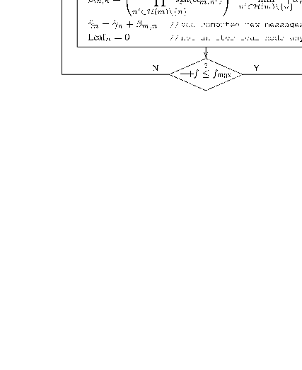
  Its implementation is represented at figure 3. We use a mixed scheduling with variable decoding parallelism, as explained in section II.

  • $\bullet$

    On top of the iteration loop we placed the hard bits computation and check nodes verification modules. This is justified by the fact that the reliability function $\bar{f}$ makes use of parity check values $\sigma_{m}$.

  • $\bullet$

    They are followed by the reliabilities computation module. It computes check nodes reliabilities and, accordingly, places check nodes in reliability sets $C_{f}$. Besides, it also set leaf flags of variable nodes ($\mbox{\rm Leaf}_{n}$) to $1$: at this moment any variable node can potentially have iteration leaf copies in different computation trees in which it appears.

  • $\bullet$

    The processing loop is placed at the bottom of the of the iteration loop. Subsets ${\cal C}_{f}$ are serially scheduled and check nodes inside one such a subset are processed in parallel. Each time that a new check node $m$ is processed we update the a posteriori information of variable nodes $n\in{\cal H}(m)$. This is done by withdrawing the old check-to-variable message, then computing the new one and finally adding the new message to the a posteriori information, as it is shown in the check nodes processing and a posteriori information module. Furthermore, each time a check node $m$ is processed we set leaf flags of variable nodes $n\in{\cal H}(m)$ to $0$, as they cannot anymore have iteration leaf copies in any computation tree. On top of this module we placed the variable nodes processing module. Thus, any variable-to-check message can be updated by withdrawing the corresponding check-to-variable message from the a posteriori information of the variable node. We note that this module concerns only messages sent to check nodes that are processed by the next module and that these messages are updated only if they come from variable nodes that are not leaf nodes with respect to the current iteration.

Figure 4 presents simulation results for irregular, rate $1/2$, binary LDPC codes. We observe that for high signal-to-noise ratios the Min-Sum decoding with neighborhood reliabilities reaches the performance of the Sum-Product decoding.

Neighborhood reliabilities can easily be generalized to the case of non-binary LDPC codes and the integer-valued reliability function $\bar{f}$ can be used without any modification. Figure 5 presents simulation results for irregular, rate $1/2$, LDPC codes over $\mbox{\rm GF}(8)$. Using neighborhood reliabilities the Min-Sum decoding performs very close to the Sum-Product decoding at high signal-to-noise ratios.

We showed that the processing order of nodes of a bipartite graph affects minimal deviations of different computation trees and therefore impacts the Min-Sum decoding performance. This motivated the introduction of neighborhood reliabilities and we developed a method that force minimal deviations to pass through reliable nodes of computation trees. We proposed an integer-valued reliability function that can be easily integrated to the Min-Sum decoding while preserving low complexity and independence on noise variance estimation errors. At our best knowledge this is the first exemple of self-correction method for the Min-Sum decoding, which applies to both binary and non-binary LDPC codes.

References

- [1] E. Boutillon, J. Tousch, and F. Guilloud. Ldpc decoder, corresponding method, system and computer program. US 2005/0138519 patent.
- [2] Y. Mao and A. H. banihashemi. A new schedule for decoding low-density parity-check codes. In Proc. IEEE GLOBECOM ’01, volume 2, pages 1007–1010, 2001.
- [3] E. Sharon, S. Litsyn, and J. Goldberger. An efficient message-passing schedule for ldpc decoding. In IEEE Proc. Conv. of Eletrical and Electronics Engeneers, pages 223–226, 2004.
- [4] N. Wiberg. Codes and decoding on general graphs. PhD thesis, Likoping University, 1996. Sweden.
- [5] J. Zhang and M. P. Fossorier. Shuffled iterative decoding. IEEE Trans. on Comm., 53(2):209–213, 2005.